Steady-state analysis and design of activated sludge processes … · · 2015-07-22Steady-state...
28
Steady-state analysis and design of activated sludge processes with a model including compressive settling Stefan Diehl 1 Jes´ us Zambrano 2 Bengt Carlsson 2 1 Centre for Mathematical Sciences, Lund University, Sweden 2 Department of Information Technology, Uppsala University, Sweden Presentation at Watermatex, Gold Coast, June 2015
Transcript of Steady-state analysis and design of activated sludge processes … · · 2015-07-22Steady-state...

Steady-state analysis and design of activated sludgeprocesses with a model including compressive settling
Stefan Diehl1 Jesus Zambrano2 Bengt Carlsson2
1Centre for Mathematical Sciences, Lund University, Sweden
2Department of Information Technology, Uppsala University, Sweden
Presentation at Watermatex, Gold Coast, June 2015

Motivation for this work
Book: Benchmarking of control strategies for wastewater treatmentplants by Gernaey, Jeppsson, Vanrolleghem and Copp (2015)
Despite successful benchmark simulation models, authors write

Motivation for this work
Book: Benchmarking of control strategies for wastewater treatmentplants by Gernaey, Jeppsson, Vanrolleghem and Copp (2015)
Despite successful benchmark simulation models, authors write
“WWTP design is mainly based on standard design rules andknowledge of human experts.”
Motivation for this work
Book: Benchmarking of control strategies for wastewater treatmentplants by Gernaey, Jeppsson, Vanrolleghem and Copp (2015)
Despite successful benchmark simulation models, authors write
“WWTP design is mainly based on standard design rules andknowledge of human experts.”
Reduced steady-state model with only few equations can bepreferable, e.g., in the first design considerations (plant area)
Previous publications: ideal point settler or hindered sedimentation
This work: include compressive settling
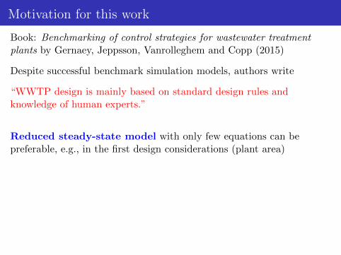
Reduced model of ASP in normal operation
zsb
Sin
S∗
S∗
S∗
Q
rQ wQ
(1 + r)Q
(1− w)Q
(r + w)Q
X∗
Xe
Xr
−H
B
biological reactor settler
z
0
hindered settling
compression
Volumetric flow rate Q [m3/h] sludge blanket level zsbSoluble substrate S [kg/m3]Particulate biomass X [kg/m3]Recycle ratio r [–]Wastage ratio w [–]

Equations for biological reactor
Completely stirred tank of volume V = ARHR
Standard mass balances:
VdS∗
dt= QSin + rQSr︸ ︷︷ ︸
in
−Q(1 + r)S∗︸ ︷︷ ︸out
− V µ(S∗, X∗)X∗
Y︸ ︷︷ ︸consumed
VdX∗
dt= rQXr −Q(1 + r)X∗ + V
(µ(S∗, X∗) − b
)X∗
Biomass decay rate bGrowth kinetics (Monod, Contois, Haldane/Andrews, Webb):
µ(S,X) = µS(1 + βS/Ki)
Ks +KCX + S + S2/Ki
For design procedure (so far): µ(S) (Monod, Haldane/Andrews)
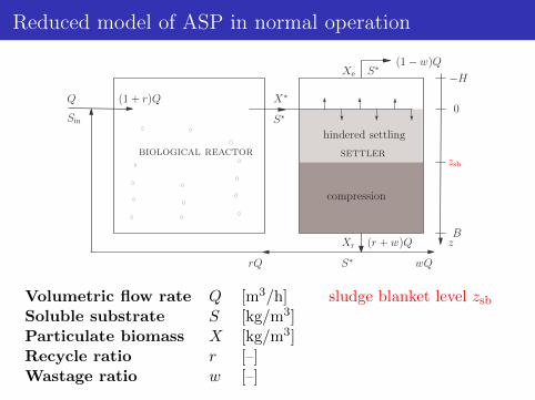
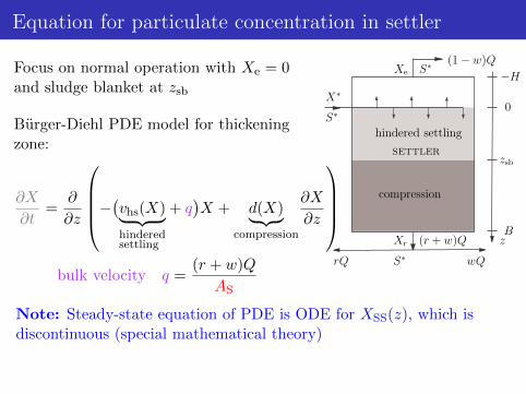
Equation for particulate concentration in settler
Focus on normal operation with Xe = 0and sludge blanket at zsb
zsb
S∗
S∗
S∗rQ wQ
(1− w)Q
(r + w)Q
X∗
Xe
Xr
−H
B
settler
z
0
hindered settling
compression

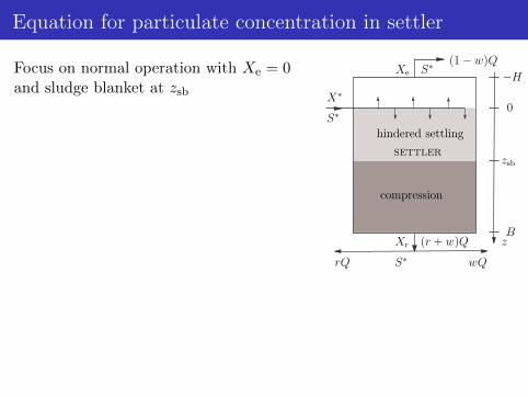
Equation for particulate concentration in settler
Focus on normal operation with Xe = 0and sludge blanket at zsb
Burger-Diehl PDE model for thickeningzone:
∂X
∂t=
∂
∂z
−(vhs(X)︸ ︷︷ ︸hinderedsettling
+ q)X + d(X)︸ ︷︷ ︸
compression
∂X
∂z
bulk velocity q =
(r + w)Q
AS
zsb
S∗
S∗
S∗rQ wQ
(1− w)Q
(r + w)Q
X∗
Xe
Xr
−H
B
settler
z
0
hindered settling
compression
Note: Steady-state equation of PDE is ODE for XSS(z), which isdiscontinuous (special mathematical theory)

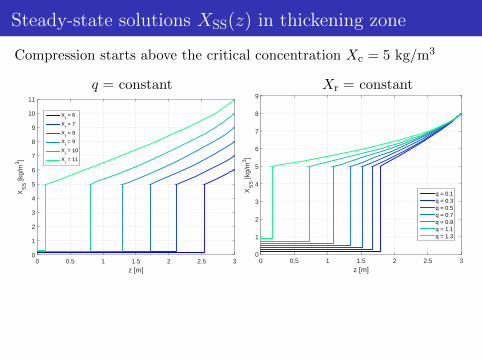
Steady-state solutions XSS(z) in thickening zone
Compression starts above the critical concentration Xc = 5 kg/m3
q = constant
z [m]0 0.5 1 1.5 2 2.5 3
XS
S [k
g/m
3 ]
0
1
2
3
4
5
6
7
8
9
10
11
Xr = 6
Xr = 7
Xr = 8
Xr = 9
Xr = 10
Xr = 11
Steady-state solutions XSS(z) in thickening zone
Compression starts above the critical concentration Xc = 5 kg/m3
q = constant Xr = constant
z [m]0 0.5 1 1.5 2 2.5 3
XS
S [k
g/m
3 ]
0
1
2
3
4
5
6
7
8
9
10
11
Xr = 6
Xr = 7
Xr = 8
Xr = 9
Xr = 10
Xr = 11
z [m]0 0.5 1 1.5 2 2.5 3
XS
S [k
g/m
3 ]0
1
2
3
4
5
6
7
8
9
q = 0.1q = 0.3q = 0.5q = 0.7q = 0.9q = 1.1q = 1.3
Observation: sludge blanket level zsb depends on q and Xr
Result: capture this relation with algebraic equation replacing ODE

Steady-state equation for settler in normal operation
Result: For a given wanted sludge blanket level zsb:
Xr = Uzsb(q) := X∞zsb
(1 +
qzsbq + qzsb
), X∞zsb , qzsb , qzsb parameters

Steady-state equation for settler in normal operation
Result: For a given wanted sludge blanket level zsb:
Xr = Uzsb(q) := X∞zsb
(1 +
qzsbq + qzsb
), X∞zsb , qzsb , qzsb parameters
The flux capacity: Φzsb(q) := qUzsb(q)
q [m/h]0 0.1 0.2 0.3 0.4 0.5 0.6 0.7 0.8
)z sb
[kg/
(m2 h)
]
0
1
2
3
4
5
6
7
8
overloaded
underloaded
zsb
= 0 m
zsb
= 1 m
zsb
= 2 m
zsb
= 3 m
Limiting flux because ofcompression!
Set of algebraic eqs for ASP insteady state
Solutions depend on r
For results and nice graphs, seepaper

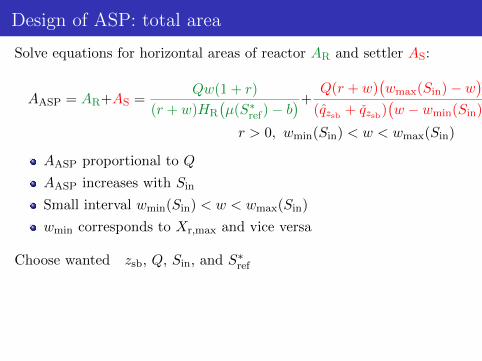
Design of ASP: total area
Solve equations for horizontal areas of reactor AR and settler AS:
AASP = AR+AS =Qw(1 + r)
(r + w)HR
(µ(S∗ref) − b
)+Q(r + w)
(wmax(Sin) − w
)(qzsb + qzsb)
(w − wmin(Sin)
)r > 0, wmin(Sin) < w < wmax(Sin)

Design of ASP: total area
Solve equations for horizontal areas of reactor AR and settler AS:
AASP = AR+AS =Qw(1 + r)
(r + w)HR
(µ(S∗ref) − b
)+Q(r + w)
(wmax(Sin) − w
)(qzsb + qzsb)
(w − wmin(Sin)
)r > 0, wmin(Sin) < w < wmax(Sin)
AASP proportional to Q
AASP increases with Sin
Small interval wmin(Sin) < w < wmax(Sin)
wmin corresponds to Xr,max and vice versa
Choose wanted zsb, Q, Sin, and S∗ref
Study AASP(r, w)

Design of ASP: total area given zsb, Q, Sin, S∗ref
Graph and contours of AASP = AASP(r, w)
21.5
r
10.5
Sin
= 0.4 kg/m3
0.0180.02
0.022
w
0.0240.026
0
1000
2000
3000
AA
SP
(r,w
) [m
2 ]
1000
1500
1500
2000
2000
2500
2500
3000
3000
3500
3500
4000
4000
0.3
0.3
0.5
0.5
0.7
0.7
0.9
0.9
0.9
Sin
= 0.4 kg/m3
r0.2 0.4 0.6 0.8 1 1.2 1.4 1.6 1.8 2
w
0.017
0.018
0.019
0.02
0.021
0.022
0.023
0.024
0.025
0.026
0.027
Dotted black curves in right plot show ratios AR/AASP
One diagram: Decide AR, AS and nominal operating point (r, w)

Main conclusions
New algebraic equation Xr = Uzsb(q) means that flux capacity dueto compressive settling easily included in analysis
Design procedure: explicit formulas — one diagram

Main conclusions
New algebraic equation Xr = Uzsb(q) means that flux capacity dueto compressive settling easily included in analysis
Design procedure: explicit formulas — one diagram
Related work: See our poster on a plug-flow reactor + settler
Thank you for your attention!

![Comparison of different fluid dynamics in activated sludge ... · dairy effluents [10-21]. Among the abovementioned processes, the activated sludge (AS) process is widely used for](https://static.fdocuments.in/doc/165x107/5f85dff14a06430d9c3028a7/comparison-of-different-fluid-dynamics-in-activated-sludge-dairy-effluents-10-21.jpg)