Steady separated flow in a linearly decelerated free stream · One of the main unsolved problems in...

J . Fluid Mech. (1973), vol. 59, part 3, pp. 513-535

Printed in Great Britain 513

Steady separated flow in a linearly decelerated free stream

By L. G. LEAL Chemical Engineering, California Institute of Technology, Pasadena, California 9 1106

(Received 7 January 1972 and in revised form 11 April 1973)

Numerical methods are used to investigate the separated flow over a finite flat plate when the flow at large distances is given by the stream function $a = - xy and the plate is situated on the x axis from - 1 to 1. The range of nominal Reynolds number is 10-800. Reduced-mesh calculations are used for fine resolution of the flow field in the immediate vicinity of the separation point. Streamlines, equivorticity lines, and shear stress and pressure gradient at the plate surface illustrate the overall structure of the flow. In each case the streamwise pressure gradient is less than that for undisturbed potential flow and the position of separation is consequently downstream of that predicted by classical boundary- layer theory. The boundary-layer structure in the vicinity of the separation point shows a direct transition between the regular upstream behaviour and Dean’s (1950) solution right at separation with no sign whatever of intermediate singular behaviour of the type predicted by Goldstein (1948). The implications of these results for the structure of high Reynolds number, steady, laminar flow are discussed.

1. Introduction One of the main unsolved problems in fluid mechanics is the proper description

of the high Reynolds number, steady, laminar motion of an incompressible fluid which exhibits boundary-layer separation. The flow field upstream of the separation point is known to be mainly inviscid and irrotational, with viscous effects confined to a very thin boundary-layer region at the surface of the body. At the separation point, however, this flow, which has hitherto closely followed the wall contours, suddenly and for no obvious reason breaks away from the wall and, downstream, the original boundary-layer fluid encompasses a region of recirculating flow whose linear dimensions are frequently comparable with the characteristic length scale of the body itself. Although the qualitative picture is thus known, the precise shape of the recirculating flow is not known and in fact a self-consistent description of the post-separation flow region has not yet been achieved for large Reynolds number R. What is worse, the recirculating eddy of unknown shape and size causes the effective body shape for the potential flow velocity field to be different from the known shape of the rigid body. Thus, strictly speaking one cannot even calculate the upstream pressure distribution which is required for the pre-separation boundary-layer solution. Finally,

F L M 33

514 L. G . Leal

although Goldstein’s (1 948) singular solution of the boundary-layer equations near a point of separation is 25 years old, its relevance to real high Reynolds number flows is still uncertain and a fully self-consistent asymptotic solution for the flow structure near a separation point has not yet been achieved. Hence the basic structure of a real, large Reynolds number, laminar flow in the vicinity of the separation point remains in doubt, in spite of the fact that the close proximity of the points of breakaway and of zero shear stress would seem to imply a strong correlation between the mechanics of the separation process and the structure of the boundary-layer solution just upstream of the separation point.

In this paper we employ numerical solutions of the two-dimensional Navier- Stokes equations for a particular separated flow problem to investigate the structure of both the post-separation recirculating eddy and the region very near to the separation point. The solutions span a nominal Reynolds number range from 10 to 800. Special techniques have been employed to achieve very fine resolution of the flow field in the vicinity of the calculated separation point. In the next two sections we briefly describe the physical problem and discuss key features of the computational methods. Subsequently, we consider the structure of the calculated flow field as a function of the Reynolds number, paying particular attention to the post-separation and separation regions as indicated above.

2. The physical problem and the basic equations The problem considered is sketched in figure 1 and consists of steady flow over

a finite flat plate which is situated from x = - 1 to x = I on the x axis (y = 0) when the stream function at large distances from the plate is given as

$km = -xy. (1)

Examination of the undisturbed velocity component parallel to the plate, is. U, 5 [a$/ay],=, = - x, shows that the problem defined by (1) is a particular example of the classical problem of boundary-layer theory studied by Howarth and others (cf. Schlichting 1968) in which it is assumed that U, = U,-axn with X increasing from zero at the leading edge. With U, = free-stream velocity at the leading edge, a = U, and n = 1, Howarth’s (1938) analysis shows that the boundary layer separates at x = 0.88 and that the boundary-layer solution becomes singular as this point is approached from the leading edge. In addition, the problem bears certain similarities to Proudman & Johnson’s (1962) analytical investigation of the boundary-layer flow developing from rest near the rear stagnation point of a circular cylinder.?

If we consider the fluid to be incompressible and Newtonian, the steady fluid motion is described by the Navier-Stokes and continuity equations

( 2 )

V.u’ = 0. (3)

p(u’ . V’) u’ = - Vp‘ + pVZu’,

t I am grateful to Prof. K. Stewartson for pointing out this similarity.

Steady separated $ow 515

FIGURE 1. The physical problem.

For simplicity, we assume the leading edge of the plate to be located at x = 1 and hence take L = I as an appropriate characteristic length. In addition, we adopt the x component of the free-stream velocity evaluated at the leading edge, U = 1 ,as the appropriate characteristic velocity scale. Thus, non-dimensionalizing (2) and (3) we obtain

u . vu = - v p + (2/R) v2u, (4)

v.u = 0, (5) where R = 2/v.

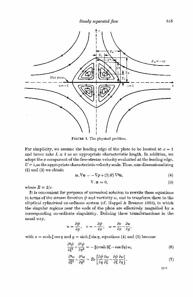
It is convenient for purposes of numerical solution to rewrite these equations in terms of the stream function $ and vorticity w , and to transform them to the elliptical cylindrical co-ordinate system (cf. Happel & Brenner 1965), in which the singular regions near the ends of the plate are effectively magnified by a corresponding co-ordinate singularity. Defining these transformations in the usual way,

a@ . av au aY ’ ax ’ ax ay)

u.=- a+ u = - - w =---

with x = cosh cos 7 and y = sinh [ sin 7, equations (4) and (5) become

33-2

516 L. G. Leal

R h a

0.5 0.3 0.2 0.2 0.2 0.15 0.2 0.15

TABLE I. Numerical parameters

x m

10.7

5.5 4.82 3.53 4-82 3.53 3-53 3.53

Corresponding boundary conditions, appropriate to the sketch of figure 1, are

$-z-sinh5cosh6cos?1sinp, w + O as [-too (0 < q < in), (8)

a@( = $- = 0 for 5 = 0 (0 < 7 G in), (9) $ = w = 0 for 7 = 0, &, all [. (10)

Since the flow is symmetric about both the x and y axes we consider only the quarter-plane x 0, y 2 0 (i.e. 0 < 7 < in).

3. The numerical solution scheme Equations (6) and (7) were recast into finite-difference form using the centred

four-point, O(h2), approximation for the Laplacian operator and the nine-point, O(h2), formula of Arakawa (1966) for the Jacobian a($, w) /a (q , [). Here h denotes the computational mesh size in the 5 , ~ plane. The Arakawa difference scheme is preferable to the standard four-point central-difference approximation for the Jacobian primarily because it exhibits enhanced stability at high Reynolds numbers (Arakawa 1966; Lilly 1965; Molenkamp 1968). The basic difference equations are lengthy and appear elsewhere (cf. Lilly 1965; Molenkamp 1968) and so are not repeated here.

Following the lead of previous investigators (cf. Dennis & Walsh 1971; Son & Hanratty 1969; Masliyah & Epstein 1970; Takami & Keller 1969), the no-slip condition a$la( = 0 at [ = 0 was transformed into a condition for vorticity at the plate surface, by applying (6) and the additional condition = 0 to evaluate the coefficients of a Taylor series expansion for $l ($I5+) in terms of $ and its normal derivatives at 6 = 0. When this expansion is carried up to terms of O(h3), the resulting condition can be written as

Miw, = - (3$hl/h2) - +M;o,, (11)

where wo and w1 are w15=o and wIteh, and M i = ~ ( c o s h 2 ~ - ~ o s 2 q ) ~ = ~ . Although the equivalent condition obtained by terminating the expansion for ?i/.l after terms O(h2) has been used before because of its greater numerical stability (Leal & Acrivos 1969), we prefer the more accurate O(h3) formula here because we are especially interested in the flow very near the plate surface.

steady separated $ow

The boundary condition (8) was approximated by setting

$ = -sinhccosh[sinrcosy

517

and o = 0 at a large value of [, which we shall denote as &,. The values of X , ( = coshe,) actually used are tabulated in table 1. The influence of & on the solution was carefully evaluated in each instance as we shall discuss in the next section. In the usual case of uniform streaming at infinity (i.e. U, = I), analogous conditions have been employed in a number of previous investigations including the recent work of Son & Hanratty (1969) and Masliyah & Epstein (1970). Takami & Keller (1969) and Leal & Acrivos (1969) both used an additional ‘wake ’ correction, corresponding to the first terms of the far-wake expansion of Imai (1951). The inclusion of such a correction is essential in principle for the case of uniform streaming at infinity because the uncorrected condition @a = y is otherwise incompatible with an overall balance of linear momentum based upon the finite drag experienced by the body. However, careful comparison of solutions calculated with and without the correction in an earlier study (Leal & Acrivos 1969) had shown that the only practical result of including the wake correction is to decrease the values of ern necessary to produce an accurate solution in the region near to the body. Although one could not perhaps have anticipated this ‘insensitivity ’ of the solution near the body to the form of the boundary condition at large distances, a partial explanation is that the major numerical errors in the ‘free- stream’ condition occur in the wake, and in this region, the Navier-Stokes equations become increasingly parabolic with increasing Reynolds number, so that these errors are not propagated very effectively back upstream towards the body.? A similar wake correction was not used in the present calculations primarily for the reason that, in this instance, the free-stream condition (8), applied at large but finite &, identically satisfies the overall linear momentum balance.

The basic difference equations were solved, for a given value of R and c,, using an iterative process which differed from that described in Leal & Acrivos (1969) mainly by the fact that, in the present calculations, the outer boundary condition (at em) was not coupled to the shear stress (vorticity) at the plate surface. The main iteration thus consisted of several sweeps through the stream function field using an over-relaxed Gauss-Seidel substitution with values of w from the previous iteration, followed by a single sweep through the vorticity field using the newly calculated values of @ and either the finite-difference form of (7) at interior points or equation (1 1) for points on the 5 = 0 boundary. The vorticity values were under-relaxed at each mesh point using the formula

= (wnew - wold) a +@old’

where 0 < a < 1. The values of a actually used are listed in table 1 (no attempt

t It should be noted, however, that when the fluid in the wake is stably stratified (as in the flow past a cooled flat plate), the basic equations in the wake region behave as a hyperbolic system owing to the presence of body force contributions and the solutions can become extremely sensitive to the conditions imposed at the downstream boundary.

518 L. G. Leal

was made to optimize these values). In order to enhance stability and accuracy further, the computations were carried out for 9, where

9 = $+sinh[cosh[sinqcosq.

Each solution was initiated by setting both $ and w equal to zero. Estimated computation times for an IBM 370-155 using the scheme described above range from several minutes for R = 10 to approximately 45 minutes for R = 800, the maximum value which we considered.

Before turning to a discussion of the calculated results, we shall describe the refinements, alluded to previously, in the general vicinity of the separation point. First of all, it was desired to magnify the region near the separation point by employing a very fine mesh. However, in view of storage limitations and excess computation time, it was not feasible to cover the whole solution field with a grid of sufficiently fine mesh. Because the position of the separation point was not known in advance it was also not feasible to use a single mesh system which had an increased density in a predetermined region. Thus, a scheme was devised in which a solution was first calculated using a constant mesh size (in the [, 7 plane) with no attempt to focus on the separation point. Subsequently, a reduced- size mesh system extending approximately 5-6 of the original mesh points in each of the upstream, downstream and cross-stream directions was superposed about the calculated separation point. Solutions of the full equations (6) and (7) were then calculated in the region of reduced mesh size, using the boundary conditions (9) and (11) at the plate surface, boundary values at the remaining boundaries which were obtained from the calculated values of $ and w in the original unreduced-mesh solution and initial values $, w = 0 at all interior mesh points. Owing to the considerably reduced mesh size and the limited domain, a simple four-point central-difference formula (cf. Leal & Acrivos 1969) was used for the Jacobian in the vorticity equation. The solutions calculated in this manner agreed very well with the corresponding solutions on the full mesh system, except very near the separation point, where minor modifications occurred. In terms of the original mesh system, the region where these apparent modifications occurred was invariably limited to a single mesh increment in any direction from the separation point. For most cases considered, the mesh (in the [, 7 plane) was reduced by a factor of four compared with the original mesh. However, in one case (R = 500) the mesh was reduced by a second factor of four, yielding an overall mesh size reduction of 16. Two different schemes were used to generate boundary values from the original solution for use in the reduced mesh calculations. In the first, the entire interior of the reduced-mesh region was covered with a mesh of size as illustrated by figure 2 (a),meaning that ‘exact ’ values of $ and o were known only at every fourthpoint of the external boundaries. Boundary values at intermediate mesh points were calculated by a standard numerical interpolation scheme. Although the solutions obtained using this method were satisfactory over most of the computational field, it was found that they differed locally from the unreduced-mesh solution in the two corner regions (i.e. F and its upstream counterpart). For this reason, an alternative scheme was used for the reduced-mesh calculations which are reported here. In this scheme the


X

Interpolated ,# boundaryvalue-

X . . . . . . . . . . . . . . I............. . . . . . . . . . . . . . Known

boundary value ............. . . . . . . . . . . . . . ............. \ 11

x-x

Typical computational . . . . . . . . . . . . . molecule A B C D O , . . . . . . . . . . . . .

X X . . . . . . . . . . . . Typical interior diamond

.......... X

X

X

FIGURE 2. The reduced-mesh system.

transformation from mesh size h to interior mesh size ah was accomplished in a continuous manner using appropriate difference forms of the basic equations (6) and (7) to accomplish the necessary ‘interpolation ’. A portion of the resultant mesh system is illustrated in figure 2 ( b ) . At the outermost row the original mesh was used. The next row into the reduced-mesh region was located a distance +h from this outer row, and had its mesh points separated from one another by a distance gh. The vahes of $ and o at these points were calculated using difference representations of (6) and (7) which were alternately on squares, such

520 L. G. Leal

as KLMN, and diamonds, such as PNQK. The third and subsequent rows were then situated $h apart with mesh-point spacing ih. The values of $ and w at points on row 3 were also necessarily calculated from alternating square and diamond difference representations. On the fourth and subsequent rows a straight- forward diamond representation was employed at each-point .Although this second scheme involving a continuously graded mesh is considerably more complicated to program than the simple interpolation scheme described previously, it has the appealing feature that the entire ‘interpolation’ from the large to smaller mesh is accomplished using difference representations of the equations of motion instead of a simple interpolation formula which incorporates none of the in- tended dynamical features of the problem except for those which are implicit in the ‘exact’ boundary values from the original unreduced-mesh calculation. Indeed, the discrepancies cited earlier as occurring at the corners nearest the solid boundary entirely disappeared when the graded mesh scheme was used.

The reduced-mesh calculation described above resembles (but is not precisely the same as) a ‘one-shot’ version of the alternating procedure of Schwarz for obtaining locally increased resolution for numerical computations in elliptic domains (Courant & Hilbert 1961). In the full procedure one alternates between a full-scale and an overlapping reduced-mesh region, using results of computations within a region as boundary conditions on the computations without and vice versa. To justify the procedure which we have employed, one must indicate whether the calculated flow in the original mesh system is altered by replacing its original boundary values at the plate surface with those calculated in the reduced-mesh system. This calculation was actually carried out for R = 150 and R = 500. It was found that the resulting solutions were virtually identical with the original full-mesh solutions, except at the mesh point(s) nearest to the separation point, where very minor modifications ( < 0.5 yo) occurred. Con- sequently, calculations for other values of Reynolds number were not carried beyond the first reduced-mesh ‘ correction ’.

4. Accuracy of the numerical computations The numerical computations were performed for Reynolds numbers of

10, 80, 150, 300, 500 and 800, as shown in table 1. The values of &,, the mesh size h and the relaxation factor a for the various cases are also included in table 1.

As in the calculations of Leal & Acrivos (1969), the vorticity at each mesh point oscillated with a monotonically decreasing amplitude about an apparently fixed mean. The period between a successive minimum and maximum increased from approximately 10 to 100 iterations as the calculation proceeded toward completion. The criterion for convergence was I (@new/Wold) - 1 I < at each mesh point for which IwI < Here wnew and Wold refer to vorticity values calculated at successive iterations. Since the maximum period of the vorticity oscillation was - 100 iterations, this condition ensured convergence bounds of less than 0.1 % for the vorticity at every such mesh point.

Steady separated $ow 52 1

0.000 1 0.00 I 0.0 1 I

1-2

FIGURE 3. The vorticity distribution on the plate surface as a function of distance from the leading edge (x = 1).

A number of checks were made to ensure the accuracy of the numerical solutions. First, the effects of changing the mesh size h and position of [a were investigated as already indicated. Fully converged solutions (in the sense of the previous paragraph) were calculated for R = 300 using two different values of ca, and for R = 500 using two different mesh sizes. The results, in terms of streamline and vorticity plots, are shown in figures 5 ( d ) and 5 ( e ) below. These provide a rough means of estimating the modifications resulting from changes in Em and h, re- spectively. A number of partially converged solutions (convergence bounds for o of approximately 1 %) at other values of R also showed similar small changes on increasing Em or decreasing h from their respective values as listed in table 1. Only for R = 10 and R = 80 was this programme of checks relaxed. In these cases the values of the mesh size were established from experience with the similar calculations of Leal & Acrivos (1969). It is worth noting that the unreduced mesh size at various points on the physical plane was sufficiently small, even for R = 800, to ensure 8-10 mesh points in the unseparated boundary layer at all streamwise positions.

The general lack of either experimental data or a relevant theory severely limits the number of explicit comparisons which could be used as a further check on the accuracy of the numerical solutions. However, according to the local expansion of Carrier & Lin (1948), the shear stress (or the vorticity) on the plate surface should vary as Cl/( 1 - x)a provided (1 - x)* is much less than the viscous length scale vlU. The quantity A = 8*Cl/R* has recently been evaluated as 0.755 for large R by Van de Vooren & Dijkstra (1970), who at the same time provided a convincing case for the existence of the leading-edge singularity. A log-log plot of the numerically calculated surface vorticity as a function of

522 L. G . Leal

I I I I I I I l l I I I 1 1 1 1 1 3.0 - -

-

- n

- 0.755 0.8 -

0.6 - - -

- - -

0.4 - - I I I I I l l l l I I I I I 1 1 1

n

FIGURE 4. The strength of the leading-edge singularity as a function of Reynolds number.

distance from the leading edge, shown in figure 3, exhibits a straight-line asyap- tote for small distances ( < v / U ) from the leading edge with a slope very near to the theoretical value of 4. In addition, as shown in figure 4, the coeEcient A , calculated from the best-fit straight line through the surface vorticity values, would appear to be approaching Van de Vooren & Dijkstra’s estimate of 0.755 for large R.

5. The basic flow structure Typical streamline and vorticity plots from the unreduced-mesh solutions

are shown in figures 5 (a) - ( f ) for the various values of Reynolds number listed in tabIe I. As expected, for R 80 the flow adjacent to the plate becomes detached resulting in a recirculating eddy in the corner adjacent to the vertical symmetry axis of the flow. It is of interest to consider the basic features of the flow in some detail.

5.1. The position of the separation point

First, as is evident from the streamlines of figure 5, the separation point shifts upstream as R is increased. It is not possible from our results to determine precisely the limiting value for large R since the position X, of the separation point is still changing at R = 800. According to classical boundary-layer theory a value for X , of approximately 0.83 should be expected in the limit as R --f co. As we shall see, however, the potential-flow pressure gradient (corresponding to equation (I)) on which this estimate is based overestimates considerably the values which occur in the presence of the recirculating eddy. It might, therefore, be anticipated that the actual position X , for separation would remain less than 0.88 even as R becomes very large, i.e. that the discrepancy between the classical boundary-layer result and our results at R = 800 is primarily due to the modified pressure distribution rather than the finite value of the Reynolds number. This

Steady separated flow 523

\ \ \

FIGURES 5 ( a ) - ( d ) . For legend see page 524.

524 L. G. Leal

FIGURE 5 . Streamline and vorticity plots from numerical solution. (a) R = 10. (b ) R = 80. ( c ) R = 1 5 O . ( d ) R = 300; - ,~ , ,=4%2;- - - , z , = 3 * 5 3 . ( e ) R = 500;-,h=*; _ _ _ , h = h n . (f) R = 800.

conjecture is strongly supported by boundary-layer calculations, described in detail in the appendix, in which we used the numerically calculated pressure di'stribution along the plate surface rather than the undisturbed potential flow distribution from (I). Using the pressure distribution calculated for R = 800, the predicted separation position is approximately X , = 0.72, in reasonable agreement with the corresponding value from the full equations of motion, which is shown in table 2.

5.2. The structure of the post-separation eddy

A second feature of interest in the numerical solutions is the variation with Reynolds number of the overall features of the recirculating flow region. A know- ledge of this flow structure is crucial to any attempt to develop an asymptotic model of the post-separation flow for large Reynolds number. It is useful to recall the experimental and numerical evidence from other investigations before examining this structure. We wish to call particular attention to the experiments of Acrivos and co-workers (Grove et al. 1964; Acrivos et al. 1968) on the structure of the steady laminar near-wake region in separated flows past bluff bodies; of Pan & Acrivos (1967) on the structure of the vortex system produced in a long vertical cavity by the tangential motion of a rigid surface at the top; and finally,

Xteady separated $ow 525

R x w XdX* YOlY* YWlXW - - - - 10

80 0-3 0.535 0.7 0.42 160 0.45 0.58 0.71 0-57 300 0.58 0.52 0.63 0.68 500 0.65 0.5 0.62 0.72 800 0.70 0.52 0.63 0.735

TABLE 2. Numerical results

of the numerical solutions of Takami & Keller (1966, 1969), and of Dennis and co-workers (Dennis & Chang 1970; Dennis & Walsh 1971) relating to the wake structure for steady laminar flow past a circular cylinder. All of these investigations were limited to an effective Reynolds number range of less than several hundred and hence corresponded roughly to the range of values of the present solutions. It is found in all of these configurations that for sufficiently large R (R > N 50) the recirculating region has one dimension independent of R; a second dimension in an orthogonal direction which increases linearly with increasing R; and a velocity component in the orthogonal direction which attains a constant limiting value for large R. It can thus be shown (Acrivos et al. 1965) that in each of these cases the dynamics of the recirculating region readjusts with increasing R in just such a way that the net contribution of viscous and inertia effects remains the same order of magnitude. Hence, over the range of R up to the order of several hundred, the structure of the recirculating flow region in these investigations shows no sign of becoming dominated by inviscid dynamics with viscous effects confined to thin regions at the boundaries as classical con- cepts would indicate (cf. Batchelor 1956).

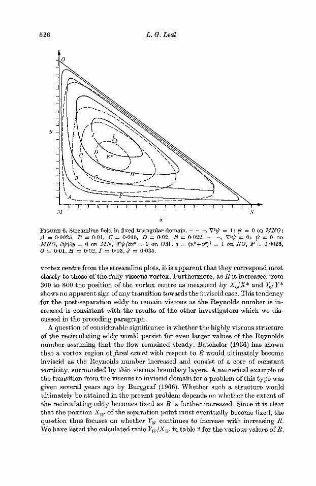
Our results also exhibit a structure of the recirculating region (for R < 800) in which viscous effects appear to retain their importance as R is increased. One way of demonstrating this is to compare the streamlines of figure 5 for R = 500 or 800 with the two sets of similar streamlines of figure 6, which were calculated by assuming a fixed shape for the recirculating region (with the same ratio of height to width) with the dynamics totally dominated in one case by viscous effects (R = 0, V4$ = 0 ) and in the other by inviscid effects (V2$ = constant). The equations and boundary conditions employed in these calculations are indicated in the legend of the figure. Comparison with the calculated streamline pattern for R = 500 or 800 suggests a closer similarity with the totally viscous model than with the inviscid one even for R = 800; this suggestion is supported quantitatively by considering the relation of the position of the vortex centre to the geometric outline of the region of recirculating flow. Thus, we determined the ratios X,/X* and &/Y* from the computed streamline plots of figure 5, where X,, Y,, X* and Y * are all defined in figure 1. The values are given for each case in table 2. These values are to be compared with those from the calculations of figure 6, which yield X,/X* N 0.4 and Y,/Y* N 0.47 for the inviscid case, and X,/X* N 0.52 and Y,/Y* N 0.63 for the viscous case. Although the values from the numerical solutions show some scatter owing to uncertainties in locating the

526 L. G . Leal

A

- - - -______- - - ------ I f l l f l l l l l l l l l l l l l l I *

I\.I N X

FIGURE 6. Streamline field in fixed triangular domain. - - -, Vz$ = 1 ; $ = 0 on MNO ; A = 0.0025, B = 0.01, C = 0.015, D = 0.02, E = 0.022. -, V4$ = 0 ; $ = 0 on MNO, a$py = 0 on M N , az$/axz = 0 on OM, q = ( . u2+vz)~ = 1 on NO, P = 0-0025, cf = 0.01, H = 0.02, I = 0.03, J = 0.035.

vortex centre from the streamline plots, it is apparent that they correspond most closely to those of the fully viscous vortex. Furthermore, as R is increased from 300 to 800 the position of the vortex centre as measured by X,/X* and Y,,/Y* shows no apparent sign of any transition towards the inviscid case. This tendency for the post-separation eddy to remain viscous as the Reynolds number is increased is consistent with the results of the other investigators which we discussed in the preceding paragraph.

A question of considerable significance is whether the highly viscous structure of the recirculating eddy would persist for even larger values of the Reynolds number assuming that the flow remained steady. Batchelor (1956) has shown that a vortex region of $xed extent with respect to R would ultimately become inviscid as the Reynolds number increased and consist of a core of constant vorticity , surrounded by thin viscous boundary layers. A numerical example of the transition from the viscous to inviscid domain for a problem of this type was given several years ago by Burggraf (1966). Whether such a structure would ultimately be attained in the present problem depends on whether the extent of the recirculating eddy becomes fixed as R is further increased. Since it is clear that the position X , of the separation point must eventually become fixed, the question thus focuses on whether Yw continues to increase with increasing R. We have listed the calculated ratio Yw/X, in table 2 for the various values of R.


1.5

1 *o

0.8 a; - s

0.6

0-4

0.2

0.0 -0.05 -0.1

0 0.2 0.4 0.6 0.8 1 .o X

FIGURE 7. Vorticity distribution on the plate surface.

The most that can be said is that the rate of increase with R is sharply decreased at the larger values of R. However, we know of no other example of a physically unconstrained closed-streamline flow which shows even the slightest indication of a viscous to inviscid vortex transition.

5.3. Shear stress and pressure distributions along the plate surface Before turning to the structure of the flow near to the separation point, it is useful t o consider the surface stress and pressure distributions from the unreduced-mesh solutions. We have plotted in figure 7 the wall shear stress, normalized by R*, as a function of position on the plate surface. Also included is the corresponding surface shear stress evaluated according to the Howarth boundary-layer solution. The chief feature of significance is the rate of change of 7 with distance as the separation point is approached. In contrast to the classical Howarth boundary-layer solution where the rate of change of T with x becomes infinite as x --f X,, dr/dx is clearly finite for each of the computed cases. This

528 L. C. Leal

0 0.2 0.4 0.6 0.8 I .o X

FIGURE 8. Dimensionless pressure gradient on the plate surface.

result, if truly representative of the flow structure near separation at large Reynolds number, would obviously have important implications for theoretical understanding of the separation process. It is, of course, possible that the regularity observed here is either a result of the fact that the Reynolds numbers are not sufficiently large to reveal the true asymptotic behaviour of the flow for R -+ co, or that the unreduced-mesh system does not provide an adequate resolution of the flow region near the separation point. We shall consider both pos sibilities in more detail in the next section.

The dimensionless pressure gradient along the plate surface is plotted as a function of position in figure 8. Here the pressure is non-dimensionalized with respect to +pU2, where U = 1 is the free-stream velocity component tangential to the plate evaluated at the leading edge x = 1. Also shown is the corresponding pressure gradient which would exist at the plate surface in the absence of viscous effects if the stream function for the free stream were = -xy. Clearly there is a considerable reduction of the streamwise pressure gradient associated with the separation of the boundary-layer flow. The nearly constant pressure along the wall adjacent to the region of recirculating flow reflects the fall off of the velocities there relative to those in the free stream. However, the reduced values of the pressure gradient upstream of the separation point are almost certainly a result


of the modification of effective boundary shape by the standing eddy. As we have indicated in 9 5.1, the reduced upstream streamwise pressure gradient results in separation being delayed relative to the position predicted by classical boundary- layer theory whenthe pressure is uncorrected for the presence of the standing eddy. The abrupt reversal evident near the leading edge for dpldx can be traced to the local viscous effects considered by Carrier & Lin (1948).

6. The flow structure very near to the separation point Early interest in the local structure of boundary-layer flow at separation was

prompted in part by the practical observation that numerical solution techniques which were adequate upstream seemed invariably to break down as the separation point was approached (cf. Howarth 1938). In spite of considerable discussion by various investigators, it was not until 1948 that Goldstein offered an explanation for these difficulties. Employing a local expansion of the boundary-lager problem about the point of vanishing shear stress, Goldstein (1948) showed that unless the local pressure distribution satisfied certain rather restrictive conditions, the shear stress must be singular at the separation point, with functional form

lim (Rh) cc (z - X,)+.

Subsequent investigations, particularly the refined numerical calculations of Hartree (1949), Leigh (1955) and Terrill(1960), have demonstrated that the solution of the boundary-layer equations is nearly always singular when the pressure distribution is prescribed from the relevant potential-flow solution without any correction for the presence of a recirculating separated flow region. More recently, however, Catherall & Mangler (1966) have produced a numerical example of a separated boundary-layer flow in which the behaviour at separation is strictly regular. This was accomplished by prescribing the displacement thickness as a regular function of distance along the surface, with the pressure gradient treated as an unknown which was determined from the resultant solution.

The major question which has not yet been resolved is the proper interpreta- tion of the Goldstein singular solution. This may seem, at first sight, to be particularly difficult in view of the fact that the Navier-Stokes equations admit a regular solution at the point of vanishing skin friction of the form

R- tm

T c c IX-X,1

for arbitrary values of the Reynolds number (cf. Dean 1950). However, the local solutions of Dean and Goldstein are obtained from the full equations by different limiting processes (X -+ X , for fixed R versus R -+ co for fixed x ( - Xw)), SO

that each is relevant to a different region of the flow; the Dean solution applying within a viscous length scale v /U , while the Goldstein solution is valid within (small) length scales of O(L) . The simultaneous existence of these two local solutions, one regular and the other singular, is thus not contradictory. Nevertheless, there still exists the possibility that the Goldstein singular solution is not relevant to real flows. In particular, there is the possibility, suggested by the solution of

34 B L M

530 L. G . Leal

X

FIGURE 9. Reduced-mesh streamline and vorticity plot, R = 500, h = &-T.

-, streamlines, A = - 0.00015, B = - 0.00005, C = - 0.00001, D = - 0.000001,

P = -0~0000001, E = 0~0000001, P = 0*000001, c f = 0.000002.

_ _ _ , equivorticity lines, H = 1.5, I = 1-25, J = 1.0, K = 0-75, L = 0.5, M = 0-2, N = 0, 0 = -0.2.

Catherall & Mangler (1966), that the pressure distribution in any real flow may always adjust, through the interaction with the external potential flow, to be precisely that required to yield regular behaviour of the boundary-layer flow at separation. Hence, even with the assumption that the flow remains steady and laminar, the relevance of the Goldstein singular solution to any real large Reynolds number problem is still an open question.

We have noted, in the previous section, that the unreduced-mesh solutions exhibit apparently regular behaviour near the separation point in the present problem, with no sign whatever of singular behaviour of the Goldstein type up to a Reynolds number of 800. In order to obtain a greater resolution of the flow structure in the vicinity of the separation point, these unreduced-mesh solutions were used as the basis for solutions on a reduced-mesh system in the manner described in $3. We shall mainly consider the representative case R = 500 where the mesh was actually reduced twice by a factor of four, first from &?r to &r and then finally A m . In the latter instance, the distance between the nearest mesh point and the estimated position of the separation point was only O( 10-3L). This distance is sufficiently small that the true limiting behaviour of the fluid motion should be clearly evident. A typical streamline and vorticity plot for R = 500, with doubly quartered mesh, is shown in figure 9. The qualitative similarity of this case with the original plot of figure 5(e) for R = 500 is readily apparent. A point of possible misinterpretation is the fact that the @ = 0 streamline is perpendicular to the plate surface very near to the separation point. At first glance this would seem to imply that V / U -+ 03 as x --f X,,, a singular behaviour similar to that predicted from the boundary-layer solution. Hence, it

Steady separated $ow 53 1

0.1 t A .a-

0.07 1 A * .

4 0.01 a; 7; 0.007 a

- Slope= 1

0.004 7 .?A

0~001

0.0007

0.0004 I I I 1 I I I I 1

0.001 0,002 0.006 0:Ol 0.02 0.06 0.1 0.2

1% - X W I

FIGURE 10. Vorticity distribution at the plate surface as a function of distance from the separation point ; combined results for full- and reduced-mesh calculations at various Reynolds numbers.

is important to note that this vertical streamline is not due to a true singularity in the solution, but actually arises because of the inability of a finite-difference scheme to resolve details on a scale smaller than the mesh size. The streamline plots of figures 5 ( e ) and 9 show that the scale of the perpendicular section is directly proportional t o the numerical mesh size. The calculated shear stress distribution, discussed in the next paragraph, provides clear-cut evidence that the solution is not singular.

The result of most significance in the present context is the local behaviour of the skin friction near the separation point. The calculated shear stress distribution is plotted as a function of distance from the separation point in figure 10. For x - X , 2 0-02, the shear stress decreases relatively rapidly with Ix-X,I from the large upstream values near the leading edge. However, in every case, the shear stress curves pass smoothly from this upstream behaviour to a slope of unity in the range 0.001 6 x - X , 6 0.015, where calculated data points are available. Hence, the upstream flow merges smoothly into a regime corresponding to Dean’s regular solution of the full equations of motion with no evidence a t all of any intermediate regime where the Goldstein expansion is relevant, even as R is increased ! A further point of agreement with Dean’s solution may be observed in the streamline and vorticity plot of figure 9: since Dean’s solution is a local expansion, it is not possible to predict the actual streamline and vorticity pattern in detail, but it can be shown that both the @ = 0 and o = 0

34-2

532 L. G . Lea$

contours must emanate from the separation point as straight lines with the slope of the o = 0 line being precisely one third that of the $ = 0 line. Except for the poorly approximated streamline behaviour right at separation which we have already discussed, this feature of Dean’s solution is very closely approximated by the reduced-mesh numerical solutions. Hence, in all respects, the numerical solutions show a direct transition from the regular boundary-layer regime upstream to the regular regime described by Dean (1950).

The implications of these results for the large Reynolds number asymptotic flow structure are certainly not without ambiguity. In particular, we have also calculated the corresponding pressure distributions near the separation point, and these appear to be qualitatively unchanged in their functional dependence on x from the uncorrected potential flow distribution over the initial portion of the plate (though, of course, the magnitudes are decreased). Hence, Goldstein’s (1948) theory would seem to suggest that the corresponding solution of the boundary-layer equations might still be singular.? For this reason, as well as the fact that the post-separation recirculating region remains viscous, it is still necessary to consider the possibility that the lack of any indication of a ‘singular ’ regime near the separation point is simply a result of the fact, that R = 800 is not sufficiently large to exhibit this asymptotic (R -+ co) behaviour. Unfor- tunately, this possibility cannot be dealt with in a irrefutable manner since larger values of R are not economically feasible for numerical calculation at present. However, we believe that the results reported here are representative of the limiting behaviour for large R: certainly, experience with related flows suggests that the range R = 10-800 is sufficiently high to establish trends toward the ultimate limiting structure as R --f 03. For example, even at R = 80 the trend toward a standard boundary-layer structure for uniform flow past a flat plate is clearly evident in similar numerical solutions even though the numerical calculations do not agree quantitatively with the boundary-layer result8 until larger Reynolds numbers (cf. Dennis & Dunwoody 1966). If Goldstein’s boundary- layer expansion at X , were relevant to the real flow at large R we should have expected that this would become evident in the numerical solutions for R as large as 800. However, a natural question is whether it is self-consistent for R = 800 to be large with respect to the structure of the pre-separation boundary layer while the flow in the recirculating eddy is still highly viscous. In partial response, it should be noted that other flows, such as the steady streaming motion past a circular cylinder, have also been found experimentally which exhibit a highly viscous structure for the recirculating eddy at Reynolds numbers of several hundred, while still showing qualitative agreement with large Reynolds number boundary-layer structure in the pre-separation portion of the near-body flow. For example, Acrivos et al. (1968) find that the measured shear stress distribution

-f In fact, the boundary-layer solutions calculated (see appendix) using the numerically determined pressure distributions do show apparent singular behaviour. However, as one of the referees has pointed out, this result is most probably without any real significance since curve-fitted pressure distributions subject to numerical inaccuracies are extremely unlikely to satisfy precisely the very specific conditions required for regular behaviour.

Steady separated flow

1.0 - boundary-layer 1 1 -

- solution r - - - - Z - _-----

I I I l l -

- /*--- - 0.5 - ‘ Boundary-layer

/ //< - 0.4 - solution, using Numerical -

pressure profiles ,’ solution - from numerical ’ (Table 2) solutions

/

xw 0.3 -

0.2 - -

0.1 I I I I I I 1 I I

533

at the wetted surface of a circular cylinder for R between 64 and 150 is in excellent agreement with the shear stress predicted from boundary-layer theory using the measured pressure distribution along the cylinder surfaee, in spite of the fact that the structure of the recirculating eddy is decidedly viscous. Hence, there is not necessarily a contradiction in the possibility of large R behaviour in one region of the flow while a highly viscous structure is still maintained in another. Finally we have obtained boundary-layer solutions, as described in the appendix, using as the pressure profile the computed pressure distributions at each Reynolds number from 10 to 800. Our motivation was to use a comparison between the calculated results from the full equations at various Reynolds numbers and the corresponding boundary-layer solutions as a qualitative measure of the degree to which R,,, = 800 is actually large enough to expose the asymptotic R +- 00

behaviour of the pre-separation boundary-layer flow in the vicinity of the separation point. The most convenient results, for this purpose, are shown in figure 11, where we compare the calculated positions of separation (zero shear stress) from the boundary-layer and full numerical solutions. These show good qualitative agreement for R 2 500, hence providing perhaps the strongest evidence that R = 800 is actually large enough to exhibit asymptotic trends of the limit R -+ co for the flow structure near separation.

The calculations reported in this paper were initiated while the author was a visitor to the Department of Applied Mathematics and Theoretical Physics of the University of Cambridge. Thanks are due to this group for their hospitality and interest in this work, as well as to the director of the Computer Laboratory, who kindly provided access to the computer during this period. The author has benefited considerably during the course of this work from discussions with Professor A. Acrivos. The constructive criticisms of the various referees have led to considerable improvements in the manuscript for which the author is also grateful.

534 L. G . Leal

Appendix. Boundary-layer calculations In this appendix we describe the boundary-layer calculations based on the

numerically computed pressure distributions for R = 10-800. The method of solution used was that proposed several years ago by Smith &

Clutter (1963) in which the original boundary-layer equations are first transformed using the Palkner-Skan variables, and then solved by using a three-point backward-difference formula for the streamwise derivatives and the standard Runge-Kutta method for solving the remaining ordinary differential equation at each streamwise station. The advantage of the method is its relative simplicity and good behaviour at the leading edge. The main disadvantage is that a re- striction is placed on the minimum streamwise step size, namely X/Ax < 25, for convergence, so that one cannot proceed quite so close to the separation point as with some other methods.? Nevertheless, the nearest streamwise mesh point was always within 0.008 of the estimated separation point, certainly adequate for our purposes. The streamwise pressure gradient was determined from the results (figure 8) of the full-scale numerical calculation, using a least-squares fit to a sixth-degree polynomial. However, the full numerical results were first modified near the leading edge so as to delete the singular behaviour (corresponding t o the work of Carrier & Lin 1948) which should enter the boundary- layer calculation only at higher orders of approximation. This was accomplished by simply extrapolating the straight-line portion of the calculated pressure gradient curve (i.e. to the left of the maximum) until it intercepted the axis x = 1 (see figure 8). As a means of estimating the effect of this somewhat arbitrary procedure on the calculated results, we also used an extrapolation for R = 800 in which the pressure gradient curve was simply extended horizontally to the x = 1 axis from its calculated maximum. The position of the separation point was thereby displaced slightly further away from the leading edge, but the qualitative dependence of the shear stress on streamwise position along the plate surface was otherwise unchanged.

R E F E R E N C E S

ACRIVOS, A., LEAL, L. G., SNOWDEN, D. D. & PAN, F. 1968 Further experiments on steady separated flows past bluff objects. J . Fluid Mech. 34, 25.

ACRIVOS, A., SNOWDEN, D. D., GROVE, A. S. &PETERSON, E. E. 1965 The steady separated flow past a circular cylinder at large Reynolds numbers. J . Fluid Mech. 21, 737.

ARAKAWA, A. 1966 Computational design for long-term numerical integration of the equations of fluid motion: two dimensional incompressible flow. Part I. J . Comp. Phys. 1, 119.

BATCHELOR, G. K. 1956 On steady laminar flow with closed streamlines a t large Reynolds numbor. J . Fluid Mech. 1, 177.

BURGGRAB, 0. R. 1966 Analytical and numerical studies of the structure of steady separated flows. J . Fluid Mech. 24, 113.

CARRIER, G.F. & LIN, C. C. 1948 On the nature of the boundary layer near the leading edge of a flat plate. Quart. AppE. Math. 6, 63.

1 - 2, and hence varies from 0 to 1 along the half plate length +L measured t Here 5 from the leading edge.


CATHERALL, D. & MANGLER, K. W. 1966 The integration of the two-dimensional laminar boundary-layer equations past the point of vanishing skin friction. J . Fluid Mech. 26, 163.

COURANT, R. & HILBERT, D. 1961 Methods of Mathematical Physics, vol. 2, p. 293. Interscience.

DEAN, W. R. 1950 Note on the motion of liquid near a position of separation. Proc. Camb. Phil. SOC. 46, 293.

DENNIS, S. C. R. & CHANG, G.-Z. 1970 Numerical solutions for steady flow past a circular cylinder a t Reynolds numbers up to 100. J. Fluid Mech. 42, 471.

DENNIS, S. C. It. & DUNWOODY, J. 1966 The steady flow of a viscous fluid past a flat plate. J . Fluid Mech. 24, 577.

DENNIS, S. C. R. & WALSH, J. D. 1971 Numerical solutions for steady symmetric viscous flow past a parabolic cylinder in a uniform stream. J . Fluid Mech. 50, 801.

GOLDSTEIN, S. 1948 On laminar boundary-layer flow near a position of separation. Quart. J . Mech. Appl. Math. 1, 43.

GROVE, A. S., SHAIR, F. H., PETERSON, E. E. & ACRIVOS, A. 1964 An experimental investigation of the steady separated flow past a circular cylinder. J . Fluid Mech. 19, 60.

HAPPEL, J. & BRENNER, H. 1965 Low Reynolds Number Hydrodynamics, appendix A. Prentice-Hall.

HARTREE, D. R. 1949 A solution of the laminar boundary-layer equation for retarded flow. Aero. Res. Counc. R. &. M . no. 2426.

HOWARTH, L. 1938 On the solution of the laminar boundary-layer equations. Proc. Roy. SOC. A 164, 547.

IMAI, I. 1951 On the asymptotic behaviour of viscous fluid flow at a great distance from a cylindrical body, with special reference to Filon’s paradox. Proc. Roy. SOC. A 208, 487.

LEAL, L. G. & ACRIVOS, A. 1969 Structure of steady closed streamline flows within a boundary layer. Phys. Fluids, 12 (suppl. 11), 105.

LEIGH, D. C. F. 1955 The laminar boundary layer equation: a method of solution by means of an automatic computer. Proc. Camb. Phil. SOC. 51, 320.

LILLY, D. K. 1964 Numerical solutions for the shape-preserving two-dimensional thermal convection element. J . Atmos. Sci. 21, 83.

LILLY, D.K. 1965 On the computational stability of numerical solutions of time- dependent non-linear geophysical fluid dynamics problems. Mon. Wea. Rev. 93, 11.

MASLIYAH, J. H. & EPSTEM, N. 1970 Numerical study of steady flow past spheroids. J . Fluid Mech. 44, 493.

MOLENKAMP, C. R. 1968 Accuracy of finite-difference methods applied to the advection equation. J . Appl. Met. 7, 160.

PAN, F. & ACRIVOS, A. 1967 Steady flows in rectangular cavities. J . Fluid Mech. 28, 643. PROUDMAN, I. & JOHNSON, K. 1962 Boundary-layer growth near a rear stagnation point.

SCHLICHTING, H. 1968 Boundary-Layer Theory, 6th edn., pp. 163-164. McGraw-Hill. SMITH, A. M. 0. & CLUTTER, D. W. 1963 Solution of the incompressible laminar boundary-

layer equations. A.I.A.A. J . 1, 2002. SON, J. S. & HANRATTY, T. J. 1969 Numerical solution for the flow around a cylinder at

Reynolds numbers of 40, 200 and 500. J . Fluid Mech. 35, 369. TAEAMI, H. & KELLER, H.B. 1966 Numerical studies of steady viscous flow about

cylinders. In Numerical Solutions of Nonlinear Differential Equations (ed. H. Green- span), p. 115.

TAKAMI, H. & KELLER, H. B. 1969 Steady two-dimensional viscous flow of an incompressible fluid past a circular cylinder. Phys. Fluids, 12 (suppl. 11), 51.

TERRILL, R. M. 1960 Laminar boundary-layer flow near separation with and without suction. Phil. Trans. Roy. SOC. A 253, 55.

VAN DE VOOREN, A. I. & DIJKSTRA, D. 1970 The Navier-Stokes solution for laminar flow past a semi-iniinite flat plate. J . Engng Math. 4, 9.

J . Fluid Mech. 12, 161.

Steady separated flow in a linearly decelerated free stream · One of the main unsolved problems in...

Documents

Transcript of Steady separated flow in a linearly decelerated free stream · One of the main unsolved problems in...