Steady and unsteady numerical simulations of the flow in...

This content has been downloaded from IOPscience. Please scroll down to see the full text.

Download details:

IP Address: 129.16.64.79

This content was downloaded on 12/01/2015 at 08:02

Please note that terms and conditions apply.

Steady and unsteady numerical simulations of the flow in the Tokke Francis turbine model, at

three operating conditions

View the table of contents for this issue, or go to the journal homepage for more

2015 J. Phys.: Conf. Ser. 579 012011

(http://iopscience.iop.org/1742-6596/579/1/012011)

Home Search Collections Journals About Contact us My IOPscience

iopscience.iop.org/page/terms

http://iopscience.iop.org/1742-6596/579/1

http://iopscience.iop.org/1742-6596

http://iopscience.iop.org/

http://iopscience.iop.org/search

http://iopscience.iop.org/collections

http://iopscience.iop.org/journals

http://iopscience.iop.org/page/aboutioppublishing

http://iopscience.iop.org/contact

http://iopscience.iop.org/myiopscience

Steady and unsteady numerical simulations of the

flow in the Tokke Francis turbine model, at three

operating conditions

Lucien Stoessel1, Hakan Nilsson2

1 Master’s student, Laboratory for Hydraulic Machines, Ecole polytechnique federale deLausanne, CH-1015 Lausanne, Switzerland2 Professor, Division of Fluid Dynamics, Department of Applied Mechanics, ChalmersUniversity of Technology, SE-41296 Gothenburg, Sweden

E-mail: 1 [email protected], 2 [email protected]

Abstract. This work investigates the flow in the scale model of the high-head Tokke Francisturbine at part load, best efficiency point and high load, as a contribution to the first Francis-99workshop. The work is based on the FOAM-extend CFD software, which is a recent fork of theOpenFOAM CFD software that contains new features for simulations in rotating machinery.Steady-state mixing plane RANS simulations are conducted, with an inlet before the guide vanesand an outlet after the draft tube. Different variants of the k-ε and k-ω turbulence models areused and a linear explicit algebraic Reynolds stress model is implemented. Sliding grid URANSsimulations, using a general grid interface coupling, are performed including the entire turbinegeometry, from the inlet to the spiral casing to the outlet of the draft tube. For the unsteadysimulations, the k-ω SSTF model is implemented and used in addition to the standard k-ε model.Both the steady and unsteady simulations give good predictions of the pressure distribution inthe turbine compared to the experimental results. The velocity profiles at the runner outletare well predicted at off-design conditions. A strong swirl is however obtained at best efficiencypoint, which is not observed in the experiments. While the steady-state simulations stronglyoverestimate the efficiency, the unsteady simulations give good predictions at best efficiencypoint (error of 1.16%) with larger errors at part load (10.67%) and high load (2.72%). Throughthe use of Fourier decomposition, the pressure fluctuations in the turbine are analysed, and themain rotor-stator interaction frequencies are predicted correctly at all operating conditions.

1. IntroductionWater turbines are often used to regulate the electric grid - to balance electricity demand andsupply - since they are able to change operating point within a short time frame [1]. Thisrequires the turbines to frequently run at off-design conditions and during transients betweendifferent operating conditions. The turbines are traditionally designed for steady operation at asingle operating point, which is characterised by a stable flow with minimal swirl at the turbineoutlet. In contrast, off-design operation lead to more complex flow through the turbine andthe creation of a swirl at the runner outlet [2]. Such unsteady flow features can lead to fluid-structure interaction phenomena and oscillating forces on the runner [3, 4]. It is therefore ofimportance to investigate the flow in water turbines both at best efficency point and at off-design points. The turbines should be designed to give a high efficiency and to avoid unstable

Francis-99 Workshop 1: steady operation of Francis turbines IOP PublishingJournal of Physics: Conference Series 579 (2015) 012011 doi:10.1088/1742-6596/579/1/012011

Content from this work may be used under the terms of the Creative Commons Attribution 3.0 licence. Any further distributionof this work must maintain attribution to the author(s) and the title of the work, journal citation and DOI.

Published under licence by IOP Publishing Ltd 1

conditions. Validated numerical results can be used to extend the knowledge of the flow in theturbines, and to improve turbine design.

The present work uses the FOAM-extend fork of the OpenFOAM CFD software to studythe flow in the Tokke high-head Francis turbine model (Francis-99). FOAM-extend was referredto as OpenFOAM-dev and OpenFOAM-ext in previous work. The FOAM-extend softwareand its tools for turbomachinery simulations have been validated and applied on hydro-powersimulation cases by Nilsson [5], Petit [6] and Javadi [7]. Features for steady-state turbomachinerysimulations were developed by Beaudoin et al. [8], and tested by Page et al. [9]. Petit et al.[10] set up an open case study that proved the validity of FOAM-extend for unsteady slidinggrid simulations of swirling flows. Zhang and Zhang [11] used OpenFOAM on high-head Francisturbines, and included a model for cavitation. Recent work on Francis turbines at off-designconditions using proprietary software was performed by Nicolet et al. [4] for part load and byShingai et al. [2] for high load operation. Susan-Resiga et al. [12] also included efforts to reducethe computational effort by the use of symmetry assumptions. The use of different turbulencemodels for RANS simulations of Francis turbines was investigated and compared to experimentsat best efficiency point by Maruzewski et al. [13], while Wu et al. [14] validated their turbulencemodel in various operating conditions.

The present work examines the flow in the Tokke high-head Francis turbine model at bestefficiency point, part load and high load using several turbulence models and using two rotor-stator-interaction approaches. Steady-state simulations are performed using a single guide vaneand runner blade passage, and a mixing plane coupling between the stationary and rotating partsof the domain. Unsteady simulations are performed using all the blade passages and a slidinggeneral grid interface (GGI). The steady-state simulations include the guide vane passage, therunner, and the draft tube. The unsteady simulations also include the spiral casing and thestay vanes. The pressure and velocity distributions are compared with the experimental andnumerical results by Trivedi et al. [15], and additional experimental data that was distributedbefore the first Francis-99 workshop (www.francis-99.org).

2. Case description and numerical detailsThis section gives a brief description of the Tokke Francis turbine model case, and the numericalset-up used in the present work.

2.1. Turbine description and operating pointsThe Tokke turbine is a high-head Francis turbine with 15 full-length runner blades and 15splitter blades, with a distributor consisting of 14 stay-vanes and 28 guide-vanes. The prototypehas a runner outlet diameter D = 1.779m, a rated head of H = 377m and a rated output powerof 110MW . The model turbine, studied in the present work, has a runner outlet diameterD = 0.349m and a rated head of H = 12m. A cut view of the entire turbine geometry withall the components is shown in Figure 1. The turbine is limited by the inlet section I at theinlet of the spiral casing, and the outlet section I at the draft tube outlet. Three differentoperating points are examined; part load, best efficiency point and high load. A summary of theoperating conditions is shown in Table 1. Due to experimental flow instabilities, the data for thebest efficiency and high load conditions were given at two slightly different conditions, by theFrancis-99 workshop organizers. The present steady-state simulations are therefore conductedat the three initial operating points, as well as the two additional operating points at bestefficiency and high load. Due to the large computational cost, the unsteady simulations are onlyconducted at the initial conditions that were suggested at the time of those simulations. Thevelocity distributions of the unsteady results are thus compared with the experimental resultsat slightly different conditions.


2

Figure 1: Cut view of the entire turbine geometry.

Parameter Part load BEP 1 BEP 2 High load 1 High load 2

H [m] 12.29 11.91 12.77 11.84 12.61Q [m3/s] 0.071 0.203 0.21 0.221 0.23n [rpm] 406.2 335.4 344.4 369.6 380.4ηh,F99 = ωT/(ρQ∆p0)[−] 71.69 92.61 92.4 90.66 91.0

Table 1: Physical parameters for all operating points. BEP 2 and high load 2 correspond to thevelocity measurements close to the original BEP 1 and high load 1 conditions, and are thereforeused for the comparison of the velocity profiles.

It should be noted that in Table 1, the definition of the hydraulic efficiency neglects thepotential energy. Here ∆p0 is the difference in total pressure between the inlet section I andthe outlet section I, given by

∆p0 = p0,I − p0,I = pI − pI +ρQ2

2· ( 1

A2I

− 1

A2I

). (1)

This expression is not consistent with the definition in the IEC standard [16], which includesthe gravitational term.

2.2. Mesh and boundary conditionsOriginal block-structured hexahedral meshes were supplied by the workshop organizers. Dueto some severe imperfections, they were slightly improved in the present work. A detaileddescription of the mesh modifications is given in the Master’s thesis by Stoessel. The meshes werealso adapted for the different types of simulations. The steady-state mixing plane simulationsare conducted for one guide vane passage and one blade channel, and the complete draft tube,as seen in Figure 2. The inlet boundary condition is set at the inlet of the guide vane passage.The inlet radial velocity is given by the flow rate and the inlet cross-sectional area. The inlettangential velocity is given by a ratio of UR

Uθ= 2

3 between the radial and tangential components,approximating the angle of the stay vanes. The inlet turbulence is specified by a turbulenceintensity of 10%, and a ratio between the turbulent and laminar viscosities of νt/ν = 10. At thedraft tube outlet the static pressure is set to zero, and a zero gradient boundary condition isapplied for the other variables. A mixing plane interface is used at the runner inlet and outlet,yielding a circumferential average of the flow field [9] at those interfaces. A refined mesh is used


3

Figure 2: Computational domain for thesteady-state simulations.

Figure 3: New shape of the interface betweenrunner and draft tube, for the unsteadysimulations. Originally flat, now conical.

for the best efficiency point, with improvements in the region below the hub and between theguide vanes. The off-design meshes are kept similar as the distributed meshes, except for themost important improvements. The resulting meshes contain 3,947,947 cells at best efficiencypoint, 3,931,653 at high load and 3,929,101 at part load.

The entire turbine geometry is used in the unsteady simulations, as seen in Figure 1. Theboundary conditions are set as for the steady-state cases except that the velocity is specifiednormal to the inlet boundary. The mesh topology at the runner outlet is modified and the flatinterface between the runner outlet and the draft tube inlet is replaced by a conical surface, asseen in Figure 3. This improves the mesh quality in the region below the hub. A general gridinterface (GGI) [17] is used for the coupling between the rotating and stationary parts, allowingthe use of a sliding grid method with non-conformal meshes. The meshes consist of 12,214,685cells for the best efficiency point, 12,357,362 for the high load point, and 12,709,257 for the partload point. The supplied spiral casing and stay vane mesh has severe quality issues that affectthe pressure convergence and should be solved in the future by re-meshing this region.

2.3. Numerical methodThe software used for the simulations is FOAM-extend-3.0-Turbo, which is a modified versionof FOAM-extend-3.0. It includes recent turbomachinery-specific developments, such as animproved implementation of the mixing plane interface. The code is based on the finite volumemethod, and the pressure-velocity coupling is handled using the SIMPLE algorithm in all thepresent simulations. The convection terms are discretised with a second-order linear upwindscheme.

For the steady-state simulations, a solver that uses multiple rotating frames of references(MRF) is chosen to mimic the behaviour of a rotating runner. A mixing plane is appliedbetween stationary and rotating parts of the domain. Different schemes are available inFOAM-extend-3.0-Turbo to link the flow variables on either side of the mixing plane interface.For the best efficiency point simulations, the fluxAveragingAdjustMassFlow scheme is usedfor the velocity, where the values are adjusted to guarantee a conserved mass flow. Ascheme based on a zero gradient boundary condition, preserving a corrrect mean value, calledzeroGradientAreaAveragingMix is used for the pressure. At off-design, the default areaAveragingscheme is used for all variables. All variables are solved with a stabilised bi-conjugate gradientmethod and a diagonal incomplete LU-decomposition for preconditioning.


4

The unsteady simulations are performed with a solver that allows a physical rotation ofthe rotating part of the domain, and a coupling between the stationary and rotating parts ofthe domain with a GGI interface. The pressure is solved with a conjugate gradient methodand diagonal incomplete Cholesky preconditioning, while the other variables are solved using abi-conjugate gradient method with diagonal incomplete LU-decomposition for preconditioning.The time step corresponds to 0.25◦ of runner rotation, yielding maximum CFL numbers of about4.5, 2.85 and 2.27 for best efficiency, part load and high load, respectively.

2.4. Turbulence modelsThe turbulence models used for steady-state simulations are the standard k-ε, RNG k-ε,realizable k-ε and k-ω SST. In addition, the linear explicit algebraic Reynolds stress model(EARSM) proposed by Wallin [18, paper 6, 196-199] was implemented and tested. For theunsteady simulations, the standard k-ε and the k-ω SSTF model developed by Gyllenramand Nilsson [19] are compared. All of the turbulence models use standard high-Reynolds wallfunctions.

3. ResultsThe results are here evaluated, based on the hydraulic efficiency, the static pressure and velocitydistributions, and the pressure and torque fluctuations.

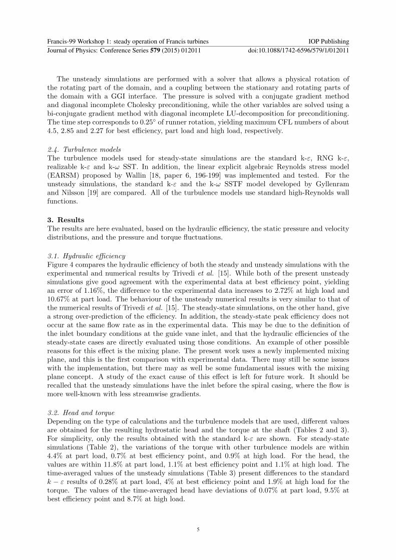
3.1. Hydraulic efficiencyFigure 4 compares the hydraulic efficiency of both the steady and unsteady simulations with theexperimental and numerical results by Trivedi et al. [15]. While both of the present unsteadysimulations give good agreement with the experimental data at best efficiency point, yieldingan error of 1.16%, the difference to the experimental data increases to 2.72% at high load and10.67% at part load. The behaviour of the unsteady numerical results is very similar to that ofthe numerical results of Trivedi et al. [15]. The steady-state simulations, on the other hand, givea strong over-prediction of the efficiency. In addition, the steady-state peak efficiency does notoccur at the same flow rate as in the experimental data. This may be due to the definition ofthe inlet boundary conditions at the guide vane inlet, and that the hydraulic efficiencies of thesteady-state cases are directly evaluated using those conditions. An example of other possiblereasons for this effect is the mixing plane. The present work uses a newly implemented mixingplane, and this is the first comparison with experimental data. There may still be some issueswith the implementation, but there may as well be some fundamental issues with the mixingplane concept. A study of the exact cause of this effect is left for future work. It should berecalled that the unsteady simulations have the inlet before the spiral casing, where the flow ismore well-known with less streamwise gradients.

3.2. Head and torqueDepending on the type of calculations and the turbulence models that are used, different valuesare obtained for the resulting hydrostatic head and the torque at the shaft (Tables 2 and 3).For simplicity, only the results obtained with the standard k-ε are shown. For steady-statesimulations (Table 2), the variations of the torque with other turbulence models are within4.4% at part load, 0.7% at best efficiency point, and 0.9% at high load. For the head, thevalues are within 11.8% at part load, 1.1% at best efficiency point and 1.1% at high load. Thetime-averaged values of the unsteady simulations (Table 3) present differences to the standardk − ε results of 0.28% at part load, 4% at best efficiency point and 1.9% at high load for thetorque. The values of the time-averaged head have deviations of 0.07% at part load, 9.5% atbest efficiency point and 8.7% at high load.


5

0.2 0.3 0.4 0.5 0.6 0.7 0.8 0.9 1 1.1 1.270

75

80

85

90

95

100

105

QED

/QED, BEP

ηh,F

99 [%

]

Steady k−ω SST

Steady Realizable k−ε

Steady RNG k−ε

Steady Standard k−ε

Steady Linear EARSM

Unsteady Standard k−ε

Unsteady k−ω SSTF

Experiments

Standard k−ε, Trivedi et al.

Figure 4: Hydraulic efficiency as a function of the relative unit flow rate, QED/QED,BEP =

(Q√HBEP )/(QBEP

√H).

Parameter Part load BEP High load

HF99 [m] 12.47 13.148 11.01T [Nm] 168.15 735.47 613.54

Table 2: Head and torque results of the steady-state standard k-ε calculations for the threeoriginal operating points.

Parameter Part load BEP High load

HF99 [m] 13.78 13.87 11.99T [Nm] 186.34 736.07 627.06

Table 3: Time-averaged head and torque results of the unsteady standard k-ε calculations forthe three original operating points.

3.3. Static pressure distributionFigure 5 shows the locations of the experimental static pressure probes, and 6 shows thecorresponding static pressure distributions. The numerical static pressure level at the outlet ofthe draft tube is adjusted to that of the experiment. Those are pI = 101.562kPa at best efficiencypoint, pI = 99.536kPa at part load, and pI = 95.977kPa at high load. The mixing planesimulations show good agreement with the unsteady simulations by Trivedi et al., regardlessof the turbulence model. The unsteady simulations give a higher static pressure on the bladesuction side, while the static pressure in the vaneless space between the guide vanes and runnerblades is closer to the experimental data. All the simulations predict a decrease in pressurebetween the P71 probe and the draft tube, while the experiment shows a slight increase. Thisindicates that certain phenomena occurring at the runner outlet are not represented the sameway in the experiment and in the numerical simulations. Figure 7 gives an overview of the staticpressure distribution in the symmetry plane of the draft tube. The static pressure probes, DT11and DT21, are located on opposite walls just below the upper velocity measurement section.A significant reduction in static pressure is observed at the centerline, and its predicted widthmust be very important for the static pressure at the walls in that region.

Figure 8 shows that all numerical pressure distributions at part load agree to a high degree,and follow a similar trend as the experimental data. Figure 9 shows that there is no local region


6

Figure 5: Locations of the static pressure probes in the guide vane cascade, runner and drafttube (illustration taken from the Francis-99 workshop website with kind permission of Prof.M.Cervantes).

of reduced pressure at the centerline in this case, and the all the numerical results do predicta similar static pressure increase between P71 and the draft tube probes as the experimentaldata.

Figure 10 shows that all numerical pressure distributions at high load are quite similar, andcorrespond to the experimental data except for the two probes in the draft tube. Figure 11shows that there is again a local reduction of the static pressure at the centerline which may bea cause of the discrepancy.

The static pressure level of the numerical results is set to the same level as that of theexperiment at the outlet of the draft tube. A numerical problem between probe P71 and thedraft tube probes will thus change the level of the upstram probes accordingly. For the bestefficiency and part load points, the numerically predicted static pressure at the draft tube probescorrespond quite well with the experimental value, indicating that the draft tube performanceis predicted reasonably well. Shifting the upstream points to lower values would in most casesimprove the results. This indicates that additional attention should be paid to the numericalmethods and the computational mesh in that region. On the other hand, the high load resultswould get worse with such an operation, although there is also a strong indication of problemsin that region. The curves indicate that also the performance of the draft tube may not bepredicted as well for the high load condition.

3.4. Velocity profilesThe velocity distributions in the draft tube cone were measured experimentally along two lines,located at z = −0.2434m and at z = −0.5614m respectively, shown as black lines in Figures 7,9 and 11. The experimental data presented in this section corresponds to the original operatingcondition at part load, but to the two additional operating conditions at best efficiency and highload. The steady-state results are taken from the same conditions as the experimental data,while the unsteady results are taken from the original conditions.

Figure 12 shows the velocity distributions for the best efficiency point. All numerical resultsshow a strong swirl near the axis of rotation which is not present in the experiments. Thisis related to the local reduction in the static pressure at the centerline, as discussed forFigure 7. The velocity distributions at the second measurement line shows that the swirl is


7

VL01 P42 S51 P71 DT11 DT2190

100

110

120

130

140

150

160

170

180

190

Pressure sensor

<p>

[kP

a]

Steady k−ω SSTSteady Realizable k−εSteady RNG k−εSteady Standard k−εSteady Linear EARSMUnsteady Standard k−εUnsteady k−ω SSTFExperiments, Trivedi et al.Standard k−ε, Trivedi et al.

Figure 6: Static pressure distribution at bestefficiency point.

Figure 7: Static pressure distribution at thesymmetry plane of the draft tube cone fora steady-state simulations at best efficiencypoint. The black lines indicate the locationof the velocity measurement sections.

VL01 P42 S51 P71 DT11 DT2180

90

100

110

120

130

140

150

160

170

180

190

Pressure sensor

<p>

[kP

a]

Steady k−ω SSTSteady Realizable k−εSteady RNG k−εSteady Standard k−εSteady Linear EARSMUnsteady k−εUnsteady k−ω SSTFExperiments, Trivedi et al.Standard k−ε, Trivedi et al.

Figure 8: Static pressure distribution at partload.

Figure 9: Static pressure distribution at thesymmetry plane of the draft tube cone for asteady-state simulations at part load. Theblack lines indicate the location of the velocitymeasurement sections.

still over-predicted by the steady-state simulations, while the unsteady profile approaches theexperimental data. The numerical axial velocity distributions agree well with the experimentaldata over most of the draft tube width, except for the region near the rotation axis. At thefirst line, only the unsteady standard k-ε simulation predicts the recirculation zone below thehub correctly, while it is under-predicted by the steady simulations and over-predicted by theunsteady k-ω SSTF results. All simulations strongly over-predict this wake region at the secondline, especially the steady EARSM and the unsteady simulations, and only the steady realizablek-ε simulation gives a correct width of the recirculation zone at this location.

Figure 13 shows that there is a strong swirl near the draft tube walls at the part load condition.


8

VL01 P42 S51 P71 DT11 DT2190

100

110

120

130

140

150

160

170

180

190

Pressure sensor

<p>

[kP

a]

Steady Realizable k−εSteady RNG k−εSteady Standard k−εUnsteady k−εUnsteady k−ω SSTFExperiments, Trivedi et al.Standard k−ε, Trivedi et al.

Figure 10: Static pressure distribution at highload.

Figure 11: Static pressure distribution at thesymmetry plane of the draft tube cone for asteady-state simulations at high load. Theblack lines indicate the location of the velocitymeasurement sections.

−1 −0.8 −0.6 −0.4 −0.2 0 0.2 0.4 0.6 0.8 1

−0.5

−0.4

−0.3

−0.2

−0.1

0

0.1

0.2

0.3

0.4

0.5

x/Rref

C/U

ref

Cz − Experiment

Cθ − Experiment

Cz − k−ω SST

Cz − Realizable k−ε

Cz − RNG k−ε

Cz − Standard k−ε

Cz − Linear EARSM

Cz − Unst. Std. k−ε

Cz − Unst. k−ω SSTF

Cθ − k−ω SST

Cθ − Realizable k−ε

Cθ − RNG k−ε

Cθ − Standard k−ε

Cθ − Linear EARSM

Cθ − Unst. Std. k−ε

Cθ − Unst. k−ω SSTF

(a) Line 1.

−1 −0.8 −0.6 −0.4 −0.2 0 0.2 0.4 0.6 0.8 1

−0.5

−0.4

−0.3

−0.2

−0.1

0

0.1

0.2

0.3

0.4

0.5

x/Rref

C/U

ref

Cz − Experiment

Cθ − Experiment

Cz − k−ω SST


Cz − RNG k−ε


Cz − Linear EARSM



Cθ − k−ω SST


Cθ − RNG k−ε





(b) Line 2.

Figure 12: Dimensionless velocity distributions in the draft tube cone at the best efficiencypoint. Cz: axial. Cθ: tangential. Note that the unsteady simulations were conducted at aslightly different operating condition than that of the experiment.

Most of the flow is passing in this region, while there is a stagnation with some back-flow in therest of the cross-section. This recirculation region is clearly visible on the pressure contours inFigure 9, as a large low pressure region that extends over a large part of the draft tube width.These phenomena are well captured both by the steady and unsteady simulations. The steadyk-ω SST gives the best prediction at the first line. The best agreement at the second line isgiven by the steady-state standard and RNG k-ε simulations, and those models give reasonableresults also at the first line.

Figure 14 shows that the axial velocity distributions correspond well to the measurementsin a large portion of the draft tube at high load. However, all numerical results predict a


9

−1 −0.8 −0.6 −0.4 −0.2 0 0.2 0.4 0.6 0.8 1

−0.5

−0.4

−0.3

−0.2

−0.1

0

0.1

0.2

0.3

0.4

0.5

x/Rref

C/U

ref

Cz − Experiment

Cθ − Experiment

Cz − k−ω SST


Cz − RNG k−ε


Cz − Linear EARSM



Cθ − k−ω SST


Cθ − RNG k−ε





(a) Line 1.

−1 −0.8 −0.6 −0.4 −0.2 0 0.2 0.4 0.6 0.8 1

−0.5

−0.4

−0.3

−0.2

−0.1

0

0.1

0.2

0.3

0.4

0.5

x/Rref

C/U

ref

Cz − Experiment

Cθ − Experiment

Cz − k−ω SST


Cz − RNG k−ε


Cz − Linear EARSM



Cθ − k−ω SST


Cθ − RNG k−ε





(b) Line 2.

Figure 13: Dimensionless velocity distributions in the draft tube cone at part load. Cz: axial.Cθ: tangential.

−1 −0.8 −0.6 −0.4 −0.2 0 0.2 0.4 0.6 0.8 1

−0.5

−0.4

−0.3

−0.2

−0.1

0

0.1

0.2

0.3

0.4

0.5

x/Rref

C/U

ref

Cz − Experiment

Cθ − Experiment


Cz − RNG k−ε


Cz − Linear EARSM




Cθ − RNG k−ε





(a) Line 1.

−1 −0.8 −0.6 −0.4 −0.2 0 0.2 0.4 0.6 0.8 1

−0.5

−0.4

−0.3

−0.2

−0.1

0

0.1

0.2

0.3

0.4

0.5

x/Rref

C/U

ref

Cz − Experiment

Cθ − Experiment


Cz − RNG k−ε


Cz − Linear EARSM




Cθ − RNG k−ε





(b) Line 2.

Figure 14: Dimensionless velocity profiles in the draft tube cone at high load. Cz: axial. Cθ:tangential. Note that the unsteady simulations were conducted at a slightly different operatingcondition than that of the experiment.

much stronger on-axis recirculation than in the experiment. The predicted swirl behaves asthe experimental, but is overestimated by all models. This swirl is then attenuated until thesecond measurement lines, but is still larger than the experimental one. The RNG k-ε and linearEARSM results show some unexpected variations in the radial direction, which is probably dueto numerical instability.

3.5. Pressure and torque fluctuationsThe pressure and torque fluctuations of the unsteady simulations are analysed using discrete fastFourier transform. Only the results for standard k-ε are shown here. The frequency spectra ofthe pressure fluctuations at the best efficiency point are shown in Figure 15. The fluctuations inthe vaneless space contain a frequency of 14.9n. This is also found in the experimental results,


10

010

2030

4050

6070

VL01

P42

S51

P71

DT11

DT21

0

0.2

0.4

0.6

0.8

1

1.2

1.4

Normalised frequency f/n [−]Pressure sensor

∆ p

(f)

[kP

a]

Figure 15: Frequency spectra of the pres-sure fluctuations at best efficiency point, nor-malised by the runner rotation frequency. Un-steady k-ε.

0 10 20 30 40 50 60 700

0.5

1

1.5

2

2.5

3

3.5x 10

−4

Normalised frequency f/n [−]

|∆ T

(f)

/ <

T>

|Figure 16: Frequency spectrum of the axialtorque at best efficiency point, normalised bythe runner rotation frequency. Unsteady k-ε.

and corresponds to the full blade passing frequency. It shows that the splitter blades do not giveexactly the same upstream imprint on the pressure distribution as the full blades. A harmoniccorresponding to the total number of runner blades is found at 31.2n. The correspondingexperimental peak is at 29.6n. The pressure on the blade surface shows a strong oscillationwith a frequency of 29.1n. The corresponding experimental peak is at 27.7n. This frequencycorresponds to the blades passing the 28 guide vanes. A series of peaks on the blade surfaceslocated between 17.8n and 18n which is measured experimentally is not found in the simulations.On the other hand, the frequency located at 62.3n, in the vane-less space and in the draft tube,is found in the numerical results but is not present in the measurements. Figure 16 shows thataxial torque oscillations occur with the main peak at 31.2n, corresponding to the total numer ofrunner blades, and a small peak at 15.6n, corresponding to the full blade passage. An additionalpeak is observed at 62.3n, corresponding to the high-frequency pressure fluctuations predictedat all sensor locations, which are not observed experimentally.

The frequency spectrum of the pressure fluctuations at part load is presented in Figure17. In the vaneless space, the passing frequency of the full blades is observed at 15.4n,corresponding to the experimentally observed 15n. The frequency corresponding to the totalnumber of blades is found at 30.77n, which corresponds to the experimentally observed 30n.On the blade surface, the guide vane passing frequency predicted at 28.7n, corresponding to theexperimentally observed 28n. The experimental data shows a second peak at 29.55n, which isnot observed numerically. The experimental data also show a strong peak at 44.3n. A tendencyof such a peak is predicted numerically, but shifted to 46.1n. The draft tube probes show theblade passing frequency at 15.4n, experimentally observed at 14.8. The draft tube frequencycorresponding to the total number of runner blades is predicted at 30.8n, which corresponds totwo experimental peaks, at 29.55n and 30n. The numerically predicted frequency of 46.1n isexperimentally measured at 44.3n. A low frequency oscillation in the draft tube is observed at0.27n in the experiments, while the numerical results show one at 0.5n. However, the peak isvery weak and no clear single frequency is present. This is consistent with the observation madeby Dorfler et al. [20, pp. 40-41], that the stable vortex rope is replaced by random pulsations atvery low part load. Figure 18 again shows that axial torque oscillations occur at 30.71n. Thereis as well a harmonic at 92.13n.

Figure 19 shows the frequency spectrum of the simulated pressure fluctuations at high load.


11

010

2030

4050

60

VL01

P42

S51

P71

DT11

DT21

0

0.2

0.4

0.6

0.8

1

1.2

1.4


∆ p

(f)

[kP

a]

Figure 17: Frequency spectrum of the pressurefluctuations at part load, normalised by therunner rotation frequency. Unsteady k-ε.

0 10 20 30 40 50 60 70 80 90 1000

1

2

3

4

5

6

7

8x 10

−4


|∆ T

(f)

/ <

T>

|Figure 18: Frequency spectrum of the axialtorque at part load, normalised by the runnerrotation frequency. Unsteady k-ε.

020

4060

80100

VL01P42

S51P71

DT11DT21

0

0.5

1

1.5

2


∆ p

(f)

Figure 19: Frequency spectrum of the pressurefluctuations at high load, normalised by therunner rotation frequency. Unsteady k-ε.

0 10 20 30 40 50 60 70 80 90 1000

1

2

3

4

5

6x 10

−4 Amplitude spectrum of torque fluctuations


|∆ T

(f)

/ <

T>

|

Figure 20: Frequency spectrum of the axialtorque at high load, normalised by the runnerrotation frequency. Unsteady k-ε.

In the vaneless space, the frequencies corresponding to the full blade passage and the totalrunner blade passage are shifted from their expected values of 15n and 30n to 14.1n and 28.2n,respectively. These frequencies are not observed experimentally. The frequency of the totalnumber of runner blades is present in the draft tube at 28.2n. On the blade surface, the guidevane passing frequency is at 26.3n, while two experimental peaks are observed at 28n and 30n.The experimental frequencies at 48.7n are not present in the simulations. On the other hand,the peak at 56.4n in the vane-less space is not present in the experimental results. Figure 20shows that the axial torque fluctuations have a main peak at 28.3n, which is the same as themost significant pressure fluctuation. A minor peak is observed at 14.1n, which is also observedin the pressure data.


12

4. ConclusionsSteady-state and unsteady numerical simulations are performed at three operating conditions ofthe Tokke high-head Francis turbine model, using several turbulence models. The steady-statesimulations use a mixing plane, and the unsteady simulations use a sliding GGI interface, forthe coupling of the stationary and rotating parts of the domain. The steady-state simulationsuse a multiple frames of reference approach, and the unsteady simulations use a rotating mesh,to represent the runner rotation. A single blade passage of the guide vanes and runner bladesis used in the steady simulations, together with a cyclic GGI, while the unsteady simulationsinclude all the blades. The steady simulations have an inlet just before the guide vanes, whilethe unsteady simulations have the inlet before the spiral casing. All simulations have the outletafter the draft tube. Most of the numerical predictions show reasonable agreement with theexperimental data, with exceptions as summarized below.

The hydraulic efficiency predictions of the unsteady simulations closely correspond to thoseof previously published simulations by other authors using a proprietary CFD code. The errorcompared with the experimental data is 1.16% at the design point, 2.27% at high load, and10.67% at part load. The similar behaviour of the present and previous numerical results suggestthat there is a systematic error in the case description, the mesh, or the common methods. All ofthose were similar in the present and the previously published study. The steady-state results dohowever yield much higher errors in the prediction of the hydraulic efficiency. The losses in thespiral casing are not included in the steady-state simulations, and the choice of inlet conditionsjust before the guide vanes should be revised to investigate their effects on the predicted hydraulicefficiency. This is the main deficiency of the steady-state results. If this deficiency is removed,the fast steady-state results are as accurate as the time-consuming unsteady results as long asit is the mean flow features and engineering quantities that are of interest.

The overall behaviour of the numerically predicted static pressure distributions is very similarto the experimental ones. A main source of difference is related the region between the trailingedges of the runner blades and the first measurement point in the draft tube. The effect of themesh resolution and mesh quality in that region should be further investigated. The presentlyused turbulence models are quite similar in nature, and they may not be able to correctlycapture the effects of turbulence in that region. At high load, the draft tube pressure recoveryis predicted different than the experimental one by all simulations, including the previouslypublished simulation.

The velocity distributions are predicted reasonably similar to the experimental ones atpart load and high load. At those conditions it is mainly the width and strength of therecirculation region below the hub that differs between models and compared to the experimentaldistributions. Even furher convergence of the steady-state results, and longer simulation timesfor the unsteady results, should be considered to verify that the flow is indeed fully developedin that region. At the best efficiency condition also the tangential velocity distribution showsan unexpected and unexplainable large discrepancy compared to the experimental one. Thisbehaviour is the same for all the turbulence models used in the present work, and it is one ofthe top priorities for further investigations.

A Fourier analysis shows that the unsteady simulations are capable of resolving the mostimportant pressure and torque fluctuations. However, there is a slight frequency shift comparedto the experimental results and the expected values. The accuracy of the frequency spectrumcould be improved by choosing a smaller time step and increasing the observation period.

All turbulence models used in the present work are part of the FOAM-extend CFD codeexcept for the linear EARSM model, which is implemented in the present work. It shows similarbehaviour as the other models. A main difference is that it gives a narrower and strongerrecirculation region below the hub. The implementation should be further verified before anymajor conclusions can be drawn, and the full EARSM model should as well be investigated.


13

AcknowledgementsThe authors would like to thank the Swedish national infrastructure for computing (SNIC) andthe Chalmers centre for computational science and engineering (C3SE) for providing supportand the computational resources for this work. Professorn Nilsson is financed by the SwedishHydro Power Center (SVC). SVC was established by the Swedish Energy Agency, Elforsk,and Svenska Kraftnat together with Lulea University of Technology, the Royal Institute ofTechnology, Chalmers University of Technology, and Uppsala University. Our thanks go alsoto Ardalan Javadi, who contributed with his experience. Furthermore, the efforts made byMartin Beaudoin and Prof. Hrvoje Jasak for the continuous improvement of FOAM-extend forturbomachinery applications as well as the fruitful discussions are much appreciated.

References[1] Nicolet C 2007 Hydroacoustic modelling and numerical simulation of unsteady operation of hydroelectric

systems Ph.D. thesis Ecole polytechnique federale de Lausanne[2] Shingai K, Okamoto N, Tamura Y and Tani K 2014 J. Fluids Eng. 136 071105[3] Keck H and Sick M 2008 Acta Mech. 201 211 – 229[4] Nicolet C, Zobeiri A, Maruzewski P and Avellan F 2011 I. J. Fluid Mach. and Syst. 4 179 – 190[5] Nilsson H 2006 23th IAHR Symp. on Hydr. Mach. and Syst.[6] Petit O 2012 Towards full predictions of the unsteady incompressible flow in rotating machines, using

OpenFOAM Phd thesis Department of Fluid Dynamics, Chalmers University of Technology Goteborg,Sweden

[7] Javadi A 2014 Time-accurate Turbulence Modeling of Swirling Flow for Hydropower Application Licentiatethesis Department of Fluid Dynamics, Chalmers University of Technology Goteborg, Sweden

[8] Beaudoin M, Nilsson H, Page M, Magnan R and Jasak H 2014 27th IAHR Symp. on Hydr. Mach. and Syst.(Montreal, Canada)

[9] Page M, Beaudoin M and Giroux A M 2011 I. J. Fluid Mach. and Syst. 4 161–171[10] Petit O, Bosioc A I, Nilsson H, Muntean S and Susan-Resiga R F 2010 25th IAHR Symp. on Hydr. Mach.

and Syst. 12 012056[11] Zhang H and Zhang L 2012 Procedia Eng. 31 156 – 165[12] Susan-Resiga R, Muntean S, Stein P and Avellan F 2009 I. J. Fluid Mach. and Syst. 2 295 – 302[13] Maruzewski P, Hayashi H, Munch C, Yamaishi K, Hashii T, Mombelli H P, Sugow Y and Avellan F 2010

IOP Conf. Ser.: Earth Environ. Sci. 12 1–9[14] Wu Y, Liu S, Wu X, Dou H, Zhang L and Tao X 2010 IOP Conf. Ser.: Earth Environ. Sci. 12 012004[15] Trivedi C, Cervantes M J, Gandhi B and Dahlhaug O G 2013 J. Fluids Eng. 135 111102[16] IEC TC/SC 4 1999 IEC 60193 Hydraulic turbine, storage pumps and pump-turbines - Model acceptance tests

(Geneva, Switzerland: International Electrotechnical Commission)[17] Beaudoin M and Jasak H 2008 Open Source CFD International Conference 2008 (Berlin, Germany)[18] Wallin S 2000 Engineering turbulence modelling for CFD with a focus on explicit algebraic Reynolds stress

models Phd thesis Royal Institute of Technology (KTH) Stockholm, Sweden[19] Gyllenram W and Nilsson H 2008 J. Fluids Eng. 130 051401[20] Dorfler P, Sick M and Coutu A 2013 Flow-Induced Pulsation and Vibration in Hydroelectric Machinery

(London: Springer)


14

Steady and unsteady numerical simulations of the flow in...

Documents

Transcript of Steady and unsteady numerical simulations of the flow in...