Status of the SPIRE photometer data processing pipelines...

Status of the SPIRE Photometer Data Processing PipelinesDuring the Early Phases of the Herschel Mission

C. Darren Dowell1, Michael Pohlen2, 3, Chris Pearson3, 4, Matt Griffin2, Tanya Lim3, GeorgeJ. Bendo5, Dominique Benielli6, James J. Bock1, Pierre Chanial7,5, Dave L. Clements5, LucaConversi8, Marc Ferlet3, Trevor Fulton9, Rene Gastaud7, Jason Glenn10, Tim Grundy3, SteveGuest3, Ken J. King3, Sarah J. Leeks3, Louis Levenson11 Nanyao Lu12, Huw Morris3, Hien

Nguyen1, Brian O’Halloran5, Seb Oliver13, Pasquale Panuzzo7,Andreas Papageorgiou2,Edward Polehampton3,4, Dimitra Rigopoulou3, Helene Roussel14, Nicola Schneider7, BernhardSchulz12, Arnold Schwartz12, David L. Shupe12, Bruce Sibthorpe15, Sunil Sidher3, Anthony J.Smith13, Bruce M. Swinyard3, Markos Trichas5, Ivan Valtchanov8, Adam L. Woodcraft16, C.

Kevin Xu12, & Lijun Zhang12

1 Jet Propulsion Laboratory/California Institute of Technology, 4800 Oak Grove Drive,Pasadena, CA 91109, USA;

2 School of Physics and Astronomy, Cardiff University, The Parade, Cardiff, CF24 3AA, UK;3 Rutherford Appleton Laboratory, Chilton, Didcot, Oxfordshire OX11 0QX, UK;

4 Institute for Space Imaging Science, University of Lethbridge, Lethbridge, Alberta, T1K3M4, Canada

5 Imperial College London, Blackett Laboratory, Prince Consort Road, London SW7, 2AZ, UK6 Laboratoire d’Astrophysique de Marseille, UMR6110 CNRS, 38 rue F. Joliot-Curie, F-13388

Marseille, France7 Commissariat a l’Energie Atomique, Service d’Astrophysique, Saclay, 91191 Gif-sur-Yvette,

France8 ESA Herschel Science Centre, ESAC, Villanueva de la Canada, Spain

9 Blue Sky Spectroscopy Inc., Suite 9-740 4th Avenue South, Lethbridge, Alberta T1J 0N9,Canada

10 University of Colorado, Dept. of Astrophysical and Planetary Sciences, CASA 389-UCB,Boulder, CO 80309, USA

11 California Institute of Technology, 1200 E. California Blvd., Pasadena, CA 91125, USA12 NASA Herschel Science Center, IPAC, 770 South Wilson Avenue, Pasadena, CA 91125, USA

13 Astronomy Centre, Dept. of Physics & Astronomy, University of Sussex, Brighton BN19QH, UK

14 Institut d’Astrophysique de Paris, UMR7095, UPMC, CNRS, 98bis Bd. Arago, 75014 Paris,France

15 UK Astronomy Technology Centre, Royal Observatory, Blackford Hill, Edinburgh EH9 3HJ,UK

16 SUPA, Institute for Astronomy, University of Edinburgh, Blackford Hill, Edinburgh EH93HJ, UK

Further author information:C.D.D.: e-mail [email protected], telephone 1-818-393-5032M.P.: e-mail [email protected], telephone +44 (0)29 208-70168C.P.: e-mail [email protected]

Space Telescopes and Instrumentation 2010: Optical, Infrared, and Millimeter Wave,edited by Jacobus M. Oschmann Jr., Mark C. Clampin, Howard A. MacEwen, Proc. of SPIEVol. 7731, 773136 · © 2010 SPIE · CCC code: 0277-786X/10/$18 · doi: 10.1117/12.858035

Proc. of SPIE Vol. 7731 773136-1

Downloaded From: http://proceedings.spiedigitallibrary.org/ on 10/28/2016 Terms of Use: http://spiedigitallibrary.org/ss/termsofuse.aspx

ABSTRACT

We describe the current state of the ground segment of Herschel-SPIRE photometer data processing, approxi-mately one year into the mission. The SPIRE photometer operates in two modes: scan mapping and choppedpoint source photometry. For each mode, the basic analysis pipeline – which follows in reverse the effects fromthe incidence of light on the telescope to the storage of samples from the detector electronics – is essentiallythe same as described pre-launch. However, the calibration parameters and detailed numerical algorithms haveadvanced due to the availability of commissioning and early science observations, resulting in reliable pipelineswhich produce accurate and sensitive photometry and maps at 250, 350, and 500 μm with minimal residualartifacts. We discuss some detailed aspects of the pipelines on the topics of: detection of cosmic ray glitches,linearization of detector response, correction for focal plane temperature drift, subtraction of detector baselines(offsets), absolute calibration, and basic map making. Several of these topics are still under study with thepromise of future enhancements to the pipelines.

Keywords: Herschel Space Observatory, far infrared, imaging, bolometer

1. INTRODUCTION

The Herschel Space Observatory was launched on 2009 May 14, achieved first light on the way to L2 orbit overthe period 2009 June 22-24, and is expected to have cryogenic operation through early 2013.1 Herschel is a3.5 m telescope passively cooled to ∼85 K and has three instruments cooled to liquid helium temperatures andsensitive to light over the range λ = 60 to 670 μm. The SPIRE instrument consists of a three-band imagingphotometer and a two-band imaging Fourier-transform spectrometer.2 In this paper, we describe the standarddata analysis pipelines for the SPIRE photometer.

For continuum imaging, Herschel is a high background situation; at 350 μm, for example, the emission fromthe telescope is ∼30,000 times brighter than the spatial ‘confusion noise’ from the multitude of distant galaxies,blended by diffraction. The large background dictates that the continuum measurements must be comparativein nature. Some SPIRE observations use the classic technique of chopping – modulation of the signal by rapidswitching of a mirror between two positions so that the detector alternately sees source plus background andbackground only. However, this observing mode is inefficient for mapping, so its use is restricted to point sourcephotometry. For covering larger areas, and for denser sampling of the sky plane, scan mapping is used instead.During scan mapping, all instrument and telescope mirrors are held fixed with respect to each other, but theentire observatory is scanned across the sky. Scanning modulates the signal and, especially in the case of crossingscans, allows the reconstruction of accurate maps of relative flux density, but does not permit measurements ofabsolute surface brightness. Since the confusion limit can be reached rather quickly with the SPIRE photometer,many programs make scan maps much larger than the size of the focal plane detector arrays.

The SPIRE photometer has three detector arrays – 139 feedhorn-coupled bolometers at 250 μm (“PSW”), 88at 350 μm (PMW) , and 43 at 500 μm (PLW) – which observe simultaneously but are analyzed independentlyin the standard pipelines. Bolometers are well suited for making the comparative measurements described inthe previous paragraph. As described elsewhere,3 the SPIRE bolometers are read out in a way which gives thebolometer temperature (or voltage) as a function of time over the frequency range 0 to ∼5 Hz. Changes inradiation incident on the detector are registered as small changes in temperature (or voltage) in the bolometer,giving an ‘AC’ signal superposed on a large baseline (DC offset) which is a function of background radation power,detector operating temperature, and individual detector properties. The baseline must be removed in the dataanalysis. The SPIRE bolometers have very low ‘1/f ’ noise2 and can measure with background-photon-limitedsensitivity signals modulated with frequencies from ∼5 Hz to below 0.01 Hz. In addition to the bolometers, thedetector arrays contain a handful of diagnostic channels: dark detectors (bolometers not exposed to incominglight), thermistors (well heat sunk to the silicon detector wafers), and fixed resistors.

The authors of this paper overlap significantly with the SPIRE Instrument Control Centre (ICC), whichhas the responsibility to deliver scientifically useful SPIRE products to the outside observer community. Sincemost photometer observations are done in scan map mode, that is the focus of this paper. Section 2 describesthe general characteristics of the scan map pipeline, and Section 3 gives details about the modules in thatpipeline. Section 4 summarizes the pipeline for the only released SPIRE photometer observing mode that uses



chopping. Sections 5 and 6 discuss aspects in common to both pipelines. Although the large number of SPIREscientific publications to date demonstrates the quality of the products emerging from the standard pipelines,improvements can be made. Some future possibilities are discussed in Section 7.

2. SPIRE PHOTOMETER SCAN-MAP PIPELINE

The SPIRE data analysis pipelines are based on the sequence of effects on the radiometric signal as it propagatesthrough the telescope, instrument optics, detector, and electronics. The modules in each pipeline attempt to‘undo’ each effect in reverse order for the purpose of yielding the true flux densities of astronomical sources.Although in principle it is possible to construct a pipeline which solves for the thermal balance of the bolometerfor each time sample, we decided early on to implement as top priority an empirical pipeline.3 Calibrationwithin the pipeline is based on in-flight measurements approximating, to first and second order, departures fromequilibrium for a bolometer at nominal operating temperature observing nominal dark sky.

The SPIRE electronics and scan map pipeline, as originally conceived, have been described previously.3 In thispaper, we describe the updates to the pipeline as of one year after launch, illustrate some of the pipeline modulesusing flight data, describe in detail options and decisions about module operation and calibration, and finallylist elements of the pipeline which are in continuing development. We focus on the theoretical underpinnings ofthe pipeline; for the practical aspects, the reader is referred to the on-line documentation.∗

The SPIRE pipeline is operated within the Herschel Interactive Processing Environment4 (HIPE). As of thiswriting, the current version of HIPE is version 4, and our pipeline description applies to that version.

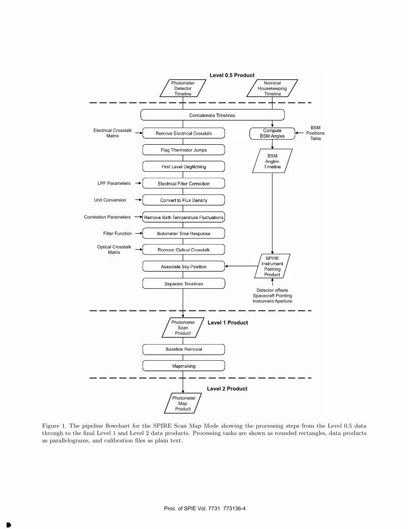
The scan map pipeline flowchart is shown in Figure 1. Changes since the prior publication3 are as follows:i) A module has been added to buffer the detector timelines to prevent edge effects, as well as a module to latertrim those buffers; ii) Deglitching and electrical crosstalk removal have been reversed, since strong glitches areobserved to produce crosstalk; and iii) A module has been added to remove residual detector baselines.

3. SCAN-MAP PIPELINE DETAILS

Our presentation of the pipeline modules here is in the order of the data analysis, which is in reverse order ofthe radiation collection, detection, analog processing, digitization, and storage. In several places, we refer to atimeline (also known as a timestream), which is a time-ordered array of a quantity such as a bolometer signal.

Most SPIRE observations are obtained with nominal detector settings, which have a flux density upper limit2

of 200 Jy. Objects an order of magnitude brighter can be observed with bright-source settings. Data processingis very similar, with the only differences being some of the calibration files and the thermometers used fortemperature drift correction (Section 3.7).

3.1 Organize Timelines, Convert to Voltage Units

Each SPIRE scan map Astronomical Observing Template (AOT; Table 1) consists of two or more scanlines, eachwith nominally constant velocity; the slews between scanlines (turnarounds); and a PCAL (internal far-infraredemission source) calibration. Only the scanlines themselves are included in the standard output data product,and each scanline is processed independently and sequentially to minimize the amount of data which must bekept in memory.

Raw telemetry forms the initial ‘Level 0’ product of the pipeline. At the ‘Level 0.5’ stage, detector andthermometer signals have been converted from raw units to voltages and temperatures, and samples have beenorganized into discrete scanline and turnaround data according to their Building Block ID (BBID). The heart ofthe scan-map pipeline is a loop over scanline BBID’s, accomplishing the analysis steps described in Sections 3.2through 3.11.

∗Herschel Observers’ Manual: http://herschel.esac.esa.int/Docs/Herschel/html/observatory.html

SPIRE Observers’ Manual: http://herschel.esac.esa.int/Docs/SPIRE/html/spire om.html

HIPE: http://herschel.esac.esa.int/HIPE download.shtml

HSPOT help: http://herschel.esac.esa.int/Docs/HSPOT/html/hspot-help.html



// Angles

/First Level Deglitching I

Electrical Filter Correction

Convert to Flux Density

Remove Bath Temperature FluctuationsJ

Bolometer Time Response

Remove Optical Crosstalk

Baseline Removal

Mapmaking

Level 2 Product

Photometer

Detector

Timeline

Nominal

Housekeeping

Timeline

BSM

Angles

Timeline

SPIRE

Instrument

Pointing

Product

Compute

BSM Angles

Photometer

Scan

Product

Photometer

Map

Product

Level 0.5 Product

Level 1 Product

Concatenate Timelines

First Level Deglitching

Electrical Filter Correction


Remove Bath Temperature Fluctuations

Bolometer Time Response


Associate Sky Position

BSM

Positions

Table

Mapmaking

Unit Conversion

Correlation Parameters

Optical Crosstalk

Matrix

LPF Parameters

Separate Timelines

Baseline Removal

Remove Electrical Crosstalk Electrical Crosstalk

Matrix

Filter Function

Flag Thermistor Jumps

Detector offsets

Spacecraft Pointing

Instrument Aperture

Figure 1. The pipeline flowchart for the SPIRE Scan Map Mode showing the processing steps from the Level 0.5 datathrough to the final Level 1 and Level 2 data products. Processing tasks are shown as rounded rectangles, data productsas parallelograms, and calibration files as plain text.



Table 1. Released SPIRE Photometer Scan Map Modes

Scan Rate Sample RateAOT Name [′′/sec] [Hz] DescriptionLarge Map (POF5) 30 or 60 18.6 minimum 2 scans; single direction (nominal or orthog.),

or cross-linked; maximum field ∼3.8◦ squared;multiple repetitions allowed

Small Map (POF10) 30 18.6 fixed, cross-linked 1×1 scan covering a field of 4′ radius;multiple repetitions allowed

SPIRE PACS Parallel 20 or 60 10.0 single direction (nominal or orthog.);(PMODE) minimum field 30′×30′

3.2 Extend Detector Timelines

Processing of timelines cut to include only the nominal on-source data (as implied in Section 3.1) has somenegative consequences. Two of the pipeline modules use Fourier techniques, which cause ringing at the edgesof the timelines if the first and last data points are not the same. The temperature drift correction may havesimilar ‘edge effects’. Also, deglitching at the edge of timelines is problematic. To circumvent these problems,each scanline is extended to include the neighboring turnaround building blocks.

3.3 Correction for Electrical Crosstalk

The module to correct for electrical crosstalk is the same as described pre-flight.3 Since the crosstalk is small(<0.1%), a ‘dummy’ (identity) matrix is used for the calibration file at the present time. However, constructinga suitable crosstalk matrix is a medium priority within the SPIRE ICC.

We are considering two methods to derive the crosstalk matrix. The first is to use cosmic ray impacts onthe bolometer webs as a source of isolated signal. A preliminary analysis of flight data indicates that crosstalkmatrix elements may be derived by accumulating many well-detected glitches in one bolometer and examiningthe average response in each other detector channel. The typical crosstalk measured using this method is oforder 0.01%-0.1%

The second method is to attribute the crosstalk to the nonzero impedance of the bias supply and to calculatethe crosstalk accordingly. All of the bolometers and diagnostic devices in a detector array share the same biassupply, and the current from one device pulls down the bias voltage for itself and the other ones. The bolometervoltage can be restored as if the bias supply had zero impedance (i.e., ‘de-crosstalked’) as follows:

V ′j = Vj +

Zj

RLj + Zj

Vb

∑i

1RLi

− ∑i

Vi

RLi

1Zb

+∑

i1

RLi

, (1)

where Vj and V ′j are the voltage of bolometer j, before and after correction; Zj is the bolometer dynamic

impedance, estimated from I-V curves; RLj is the bolometer load resistance; Vb is the bias voltage; and Zb isthe bias impedance. The observations from the cosmic ray impacts and predictions from this ‘bias droop’ modelwill be compared as a step toward providing crosstalk correction of SPIRE data.

3.4 Deglitching (First Level)

For a given SPIRE bolometer in flight, approximately 0.3% of samples are affected by obvious cosmic ray glitches.About half of the glitches are isolated to single bolometers (‘web hits’), and the remainder are concurrent withinall bolometers and thermistor channels in a detector array (‘frame hits’). The concurrent glitches were notanticipated in the pre-flight pipeline development, but have been seen in past space missions with thermaldetectors.5

Ordinary web-hit and frame-hit glitches can be removed from the data in a straightforward manner, sincethe bolometers recover quickly (Figure 2). The SPIRE scan-map pipeline currently provides two alternatives for



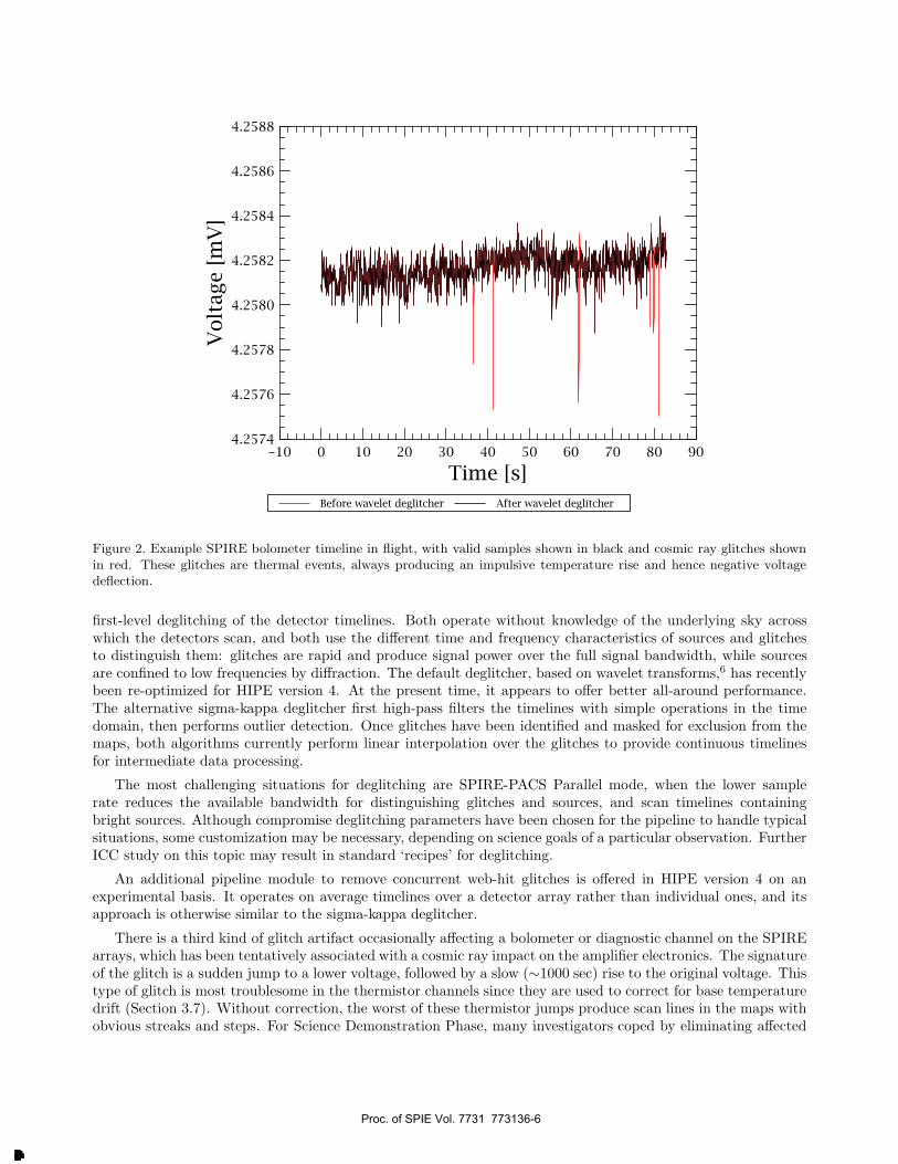
Figure 2. Example SPIRE bolometer timeline in flight, with valid samples shown in black and cosmic ray glitches shownin red. These glitches are thermal events, always producing an impulsive temperature rise and hence negative voltagedeflection.

first-level deglitching of the detector timelines. Both operate without knowledge of the underlying sky acrosswhich the detectors scan, and both use the different time and frequency characteristics of sources and glitchesto distinguish them: glitches are rapid and produce signal power over the full signal bandwidth, while sourcesare confined to low frequencies by diffraction. The default deglitcher, based on wavelet transforms,6 has recentlybeen re-optimized for HIPE version 4. At the present time, it appears to offer better all-around performance.The alternative sigma-kappa deglitcher first high-pass filters the timelines with simple operations in the timedomain, then performs outlier detection. Once glitches have been identified and masked for exclusion from themaps, both algorithms currently perform linear interpolation over the glitches to provide continuous timelinesfor intermediate data processing.

The most challenging situations for deglitching are SPIRE-PACS Parallel mode, when the lower samplerate reduces the available bandwidth for distinguishing glitches and sources, and scan timelines containingbright sources. Although compromise deglitching parameters have been chosen for the pipeline to handle typicalsituations, some customization may be necessary, depending on science goals of a particular observation. FurtherICC study on this topic may result in standard ‘recipes’ for deglitching.

An additional pipeline module to remove concurrent web-hit glitches is offered in HIPE version 4 on anexperimental basis. It operates on average timelines over a detector array rather than individual ones, and itsapproach is otherwise similar to the sigma-kappa deglitcher.

There is a third kind of glitch artifact occasionally affecting a bolometer or diagnostic channel on the SPIREarrays, which has been tentatively associated with a cosmic ray impact on the amplifier electronics. The signatureof the glitch is a sudden jump to a lower voltage, followed by a slow (∼1000 sec) rise to the original voltage. Thistype of glitch is most troublesome in the thermistor channels since they are used to correct for base temperaturedrift (Section 3.7). Without correction, the worst of these thermistor jumps produce scan lines in the maps withobvious streaks and steps. For Science Demonstration Phase, many investigators coped by eliminating affected



scan lines from the maps. However, in HIPE version 4, we expect a thermistor jump detector module to beavailable. It operates by flagging step-like glitches so that the affected portion of the thermistor signal can bedisregarded in the temperature drift correction step later on.

The scan-map pipeline currently has only a first level of deglitching. Plans for a second level of deglitchingare discussed in Section 7.

3.5 Correction for Electronic Filtering

For accuracy, we have adopted a Fourier approach to correct for the on-board analog electronics filtering. Thecorrection consists of using a Fourier transform to go from time domain to frequency domain, dividing by thefollowing transfer function (a 4-pole Bessel filter), then inverse Fourier transforming back to the time domain:

H(ω) = [1

1 + iω(42.6 × 10−3 s) + (iω)2(5 × 10−4 s2)][

11 + iω(25 × 10−3 s) + (iω)2(4 × 10−4 s2)

][1

1 + iω(10−3 s)]

(2)The buffer of time samples before and after the nominal scan (see Section 3.2) prevents edge ringing fromaffecting the maps. Following this step, the noise spectra of the bolometer signals are nearly white up to thehighest frequencies.

3.6 Convert to Flux Density

The conversion from voltage to flux density (Jy) involves two key components which are incorporated into asingle calibration file and pipeline module.7 First, the nonlinear response of the bolometer must be corrected.Second, an absolute calibrator must be used to scale linearized voltage to Jy.

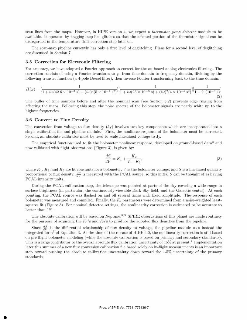
The empirical function used to fit the bolometer nonlinear response, developed on ground-based data3 andnow validated with flight observations (Figure 3), is given by:

dS

dV= K1 +

K2

V − K3, (3)

where K1, K2, and K3 are fit constants for a bolometer, V is the bolometer voltage, and S is a linearized quantityproportional to flux density. dS

dV is measured with the PCAL source, so this initial S can be thought of as havingPCAL intensity units.

During the PCAL calibration step, the telescope was pointed at parts of the sky covering a wide range insurface brightness (in particular, the continuously-viewable Dark Sky field, and the Galactic center). At eachpointing, the PCAL source was flashed on and off several times with fixed amplitude. The response of eachbolometer was measured and compiled. Finally, the Ki parameters were determined from a noise-weighted least-squares fit (Figure 3). For nominal detector settings, the nonlinearity correction is estimated to be accurate tobetter than 1% .

The absolute calibration will be based on Neptune.8, 9 SPIRE observations of this planet are made routinelyfor the purpose of adjusting the K1’s and K2’s to produce the adopted flux densities from the pipeline.

Since dSdV is the differential relationship of flux density to voltage, the pipeline module uses instead the

integrated form3 of Equation 3. At the time of the release of HIPE 4.0, the nonlinearity correction is still basedon pre-flight bolometer modeling (while the absolute calibration is based on primary and secondary standards).This is a large contributor to the overall absolute flux calibration uncertainty of 15% at present.7 Implementationlater this summer of a new flux conversion calibration file based solely on in-flight measurements is an importantstep toward pushing the absolute calibration uncertainty down toward the ∼5% uncertainty of the primarystandards.



0.0026 0.0028 0.0030 0.0032 0.0034 0.0036V

-5.0×104

-4.5×104

-4.0×104

-3.5×104

-3.0×1041/

ΔV

0.0026 0.0028 0.0030 0.0032 0.0034 0.0036V

-5.0×104

-4.5×104

-4.0×104

-3.5×104

-3.0×1041/

ΔV

PSWE2

Figure 3. Inverse bolometer response vs. bolometer voltage from a nonlinearity calibration of SPIRE bolometer PSWE2.The units are V−1 and V, respectively. The vertical axis shows the reciprocal of the bolometer response to flashes ofthe PCAL emission source (response being intrinsically negative for semiconducting bolometers); the reciprocal is usedsince it is the function dS

dVwhich is to be fit. Each point is from a different telescope pointing – low surface brightness

targets at right, and high surface brightness targets at left. The solid curve shows the best fit with Equation 3. The rightdashed vertical line shows the bolometer voltage for the Dark Sky field, and the left line shows the bolometer voltage forNeptune.

3.7 Correction for Drift in Detector Base Temperature

SPIRE is operated without temperature control of the detectors, and the bolometers experience ∼2 mK driftsoriginating at the 3He refrigerator over the course of its two day hold time. It can be shown from bolometertheory† that a base temperature fluctuation can be associated with an equivalent change in power incident onthe bolometer, so it is appropriate to apply temperature drift correction after the conversion from voltage to apower unit (Section 3.6). The effect of the temperature drift on the timelines is quite large – ∼10 Jy/mK – socorrection is essential. A passive filter with time constant ∼400 s (formed by the heat capacity of the detectorarrays and their thermal link with the fridge) attenuates the rapid temperature fluctuations from the fridge, soit is primarily frequencies <0.1 Hz which need to be corrected.

The standard pipeline removes from each bolometer a flux density which is proportional to the voltageexcursion of the functional thermistors on the same array. For purposes of low-pass filtering, the thermistorsignal is binned and fit with a cubic spline function.10 The proportionality constants are determined in aseparate, dedicated calibration measurement. Figure 4 shows an example application of this pipeline module toflight data.

3.8 Correction for Bolometer Time Filtering

Except for a handful of bolometers which are masked by the pipeline to be excluded from the maps, the radiationresponse of the bolometer itself appears to be consistent with a single-pole filter. Therefore, the timestreams are

†Bolometer equilibrium is governed by: V 2

R+ Q =

∫ T

T0G(T ′)dT ′, where V is the bolometer equilibrium voltage, R(T )

is the bolometer resistance, Q is the radiation power on the bolometer, T is the bolometer temperature, T0 is the basetemperature, and G(T ) is the bolometer thermal conductance. The SPIRE bolometers are biased with a voltage dividersuch that V = RVb

R+RL, where Vb is the fixed bias voltage and RL is the fixed load resistance. It can be shown that dV

dT0(fixed

Q) = G(T0)dVdQ

(fixed T0), i.e. base temperature fluctuations are equivalent to radiation power fluctuations except for afixed proportionality constant G(T0).



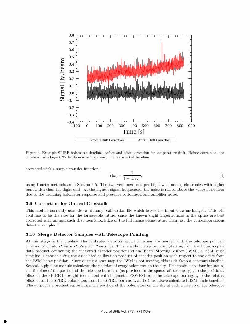
Figure 4. Example SPIRE bolometer timelines before and after correction for temperature drift. Before correction, thetimeline has a large 0.25 Jy slope which is absent in the corrected timeline.

corrected with a simple transfer function:

H(ω) =1

1 + iωτbol, (4)

using Fourier methods as in Section 3.5. The τbol were measured pre-flight with analog electronics with higherbandwidth than the flight unit. At the highest signal frequencies, the noise is raised above the white noise floordue to the declining bolometer response and presence of Johnson and amplifier noise.

3.9 Correction for Optical Crosstalk

This module currently uses also a ‘dummy’ calibration file which leaves the input data unchanged. This willcontinue to be the case for the foreseeable future, since the known slight imperfections in the optics are bestcorrected with an approach that uses knowledge of the full image plane rather than just the contemporaneousdetector samples.3

3.10 Merge Detector Samples with Telescope Pointing

At this stage in the pipeline, the calibrated detector signal timelines are merged with the telecope pointingtimeline to create Pointed Photometer Timelines. This is a three step process. Starting from the housekeepingdata product containing the measured encoder positions of the Beam Steering Mirror (BSM), a BSM angletimeline is created using the associated calibration product of encoder position with respect to the offset fromthe BSM home position. Since during a scan map the BSM is not moving, this is de facto a constant timeline.Second, a pipeline module calculates the position of every bolometer on the sky. This module has four inputs: a)the timeline of the position of the telecope boresight (as provided in the spacecraft telemetry) , b) the positionaloffset of the SPIRE boresight (coincident with bolometer PSWE8) from the telescope boresight, c) the relativeoffset of all the SPIRE bolometers from the SPIRE boresight, and d) the above calculated BSM angle timeline.The output is a product representing the position of the bolometers on the sky at each timestep of the telescope



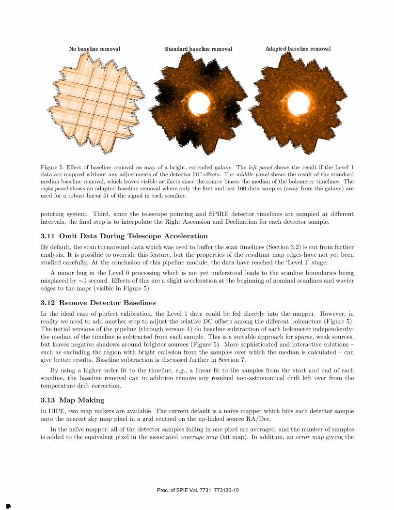
No base line removal Standard base line removal Adapted base line removal

Figure 5. Effect of baseline removal on map of a bright, extended galaxy. The left panel shows the result if the Level 1data are mapped without any adjustments of the detector DC offsets. The middle panel shows the result of the standardmedian baseline removal, which leaves visible artifacts since the source biases the median of the bolometer timelines. Theright panel shows an adapted baseline removal where only the first and last 100 data samples (away from the galaxy) areused for a robust linear fit of the signal in each scanline.

pointing system. Third, since the telescope pointing and SPIRE detector timelines are sampled at differentintervals, the final step is to interpolate the Right Ascension and Declination for each detector sample.

3.11 Omit Data During Telescope Acceleration

By default, the scan turnaround data which was used to buffer the scan timelines (Section 3.2) is cut from furtheranalysis. It is possible to override this feature, but the properties of the resultant map edges have not yet beenstudied carefully. At the conclusion of this pipeline module, the data have reached the ‘Level 1’ stage.

A minor bug in the Level 0 processing which is not yet understood leads to the scanline boundaries beingmisplaced by ∼1 second. Effects of this are a slight acceleration at the beginning of nominal scanlines and wavieredges to the maps (visible in Figure 5).

3.12 Remove Detector Baselines

In the ideal case of perfect calibration, the Level 1 data could be fed directly into the mapper. However, inreality we need to add another step to adjust the relative DC offsets among the different bolometers (Figure 5).The initial versions of the pipeline (through version 4) do baseline subtraction of each bolometer independently:the median of the timeline is subtracted from each sample. This is a suitable approach for sparse, weak sources,but leaves negative shadows around brighter sources (Figure 5). More sophisticated and interactive solutions –such as excluding the region with bright emission from the samples over which the median is calculated – cangive better results. Baseline subtraction is discussed further in Section 7.

By using a higher order fit to the timeline, e.g., a linear fit to the samples from the start and end of eachscanline, the baseline removal can in addition remove any residual non-astronomical drift left over from thetemperature drift correction.

3.13 Map Making

In HIPE, two map makers are available. The current default is a naıve mapper which bins each detector sampleonto the nearest sky map pixel in a grid centred on the up-linked source RA/Dec.

In the naıve mapper, all of the detector samples falling in one pixel are averaged, and the number of samplesis added to the equivalent pixel in the associated coverage map (hit map). In addition, an error map giving the

Proc. of SPIE Vol. 7731 773136-10


Naive Map MAD Map

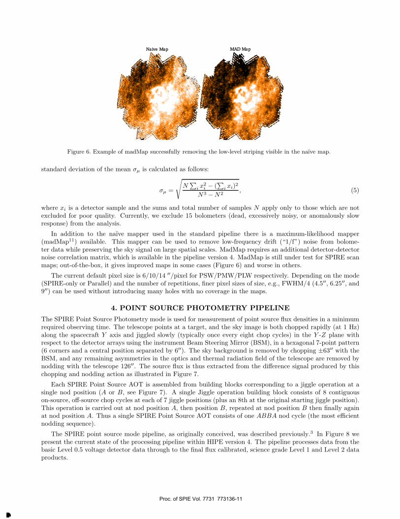
Figure 6. Example of madMap successfully removing the low-level striping visible in the naıve map.

standard deviation of the mean σμ is calculated as follows:

σμ =

√N

∑i x2

i − (∑

i xi)2

N3 − N2, (5)

where xi is a detector sample and the sums and total number of samples N apply only to those which are notexcluded for poor quality. Currently, we exclude 15 bolometers (dead, excessively noisy, or anomalously slowresponse) from the analysis.

In addition to the naıve mapper used in the standard pipeline there is a maximum-likelihood mapper(madMap11) available. This mapper can be used to remove low-frequency drift (“1/f”) noise from bolome-ter data while preserving the sky signal on large spatial scales. MadMap requires an additional detector-detectornoise correlation matrix, which is available in the pipeline version 4. MadMap is still under test for SPIRE scanmaps; out-of-the-box, it gives improved maps in some cases (Figure 6) and worse in others.

The current default pixel size is 6/10/14 ′′/pixel for PSW/PMW/PLW respectively. Depending on the mode(SPIRE-only or Parallel) and the number of repetitions, finer pixel sizes of size, e.g., FWHM/4 (4.5′′, 6.25′′, and9′′) can be used without introducing many holes with no coverage in the maps.

4. POINT SOURCE PHOTOMETRY PIPELINE

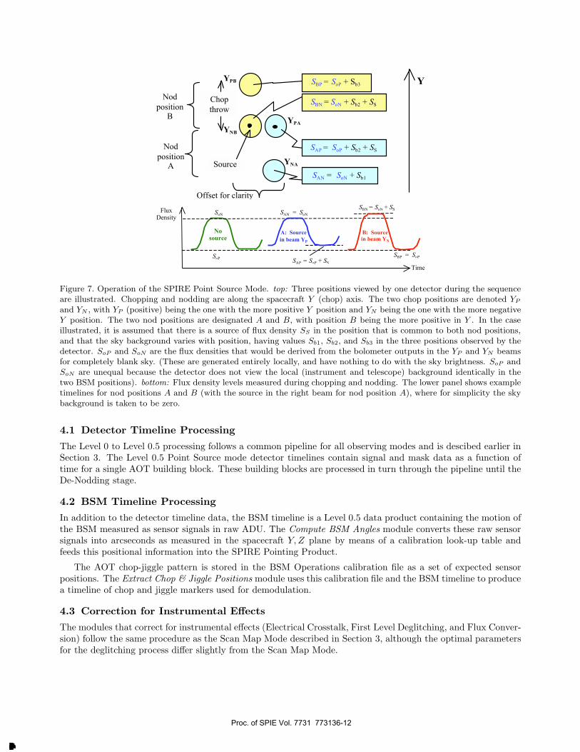
The SPIRE Point Source Photometry mode is used for measurement of point source flux densities in a minimumrequired observing time. The telescope points at a target, and the sky image is both chopped rapidly (at 1 Hz)along the spacecraft Y axis and jiggled slowly (typically once every eight chop cycles) in the Y -Z plane withrespect to the detector arrays using the instrument Beam Steering Mirror (BSM), in a hexagonal 7-point pattern(6 corners and a central position separated by 6′′). The sky background is removed by chopping ±63′′ with theBSM, and any remaining asymmetries in the optics and thermal radiation field of the telescope are removed bynodding with the telescope 126′′. The source flux is thus extracted from the difference signal produced by thischopping and nodding action as illustrated in Figure 7.

Each SPIRE Point Source AOT is assembled from building blocks corresponding to a jiggle operation at asingle nod position (A or B, see Figure 7). A single Jiggle operation building block consists of 8 contiguouson-source, off-source chop cycles at each of 7 jiggle positions (plus an 8th at the original starting jiggle position).This operation is carried out at nod position A, then position B, repeated at nod position B then finally againat nod position A. Thus a single SPIRE Point Source AOT consists of one ABBA nod cycle (the most efficientnodding sequence).

The SPIRE point source mode pipeline, as originally conceived, was described previously.3 In Figure 8 wepresent the current state of the processing pipeline within HIPE version 4. The pipeline processes data from thebasic Level 0.5 voltage detector data through to the final flux calibrated, science grade Level 1 and Level 2 dataproducts.

Proc. of SPIE Vol. 7731 773136-11


Nod

position B

Source

Nod

position A

YPB

YNB

YNA

YPA

Offset for clarity

SBP = SoP + Sb3

SBN = SoN + Sb2 + SS

SAP = SoP + Sb2 + SS

SAN = SoN + Sb1

Chop

throw

Y

A: Source

in beam YP

B: Source

in beam YN

SBP = SoP

SBN = SoN + SS Flux

Density

Time

SoN

SoP

No

source

SAN = SoN

SAP = SoP + SS

Figure 7. Operation of the SPIRE Point Source Mode. top: Three positions viewed by one detector during the sequenceare illustrated. Chopping and nodding are along the spacecraft Y (chop) axis. The two chop positions are denoted YP

and YN , with YP (positive) being the one with the more positive Y position and YN being the one with the more negativeY position. The two nod positions are designated A and B, with position B being the more positive in Y . In the caseillustrated, it is assumed that there is a source of flux density SS in the position that is common to both nod positions,and that the sky background varies with position, having values Sb1, Sb2, and Sb3 in the three positions observed by thedetector. SoP and SoN are the flux densities that would be derived from the bolometer outputs in the YP and YN beamsfor completely blank sky. (These are generated entirely locally, and have nothing to do with the sky brightness. SoP andSoN are unequal because the detector does not view the local (instrument and telescope) background identically in thetwo BSM positions). bottom: Flux density levels measured during chopping and nodding. The lower panel shows exampletimelines for nod positions A and B (with the source in the right beam for nod position A), where for simplicity the skybackground is taken to be zero.

4.1 Detector Timeline Processing

The Level 0 to Level 0.5 processing follows a common pipeline for all observing modes and is descibed earlier inSection 3. The Level 0.5 Point Source mode detector timelines contain signal and mask data as a function oftime for a single AOT building block. These building blocks are processed in turn through the pipeline until theDe-Nodding stage.

4.2 BSM Timeline Processing

In addition to the detector timeline data, the BSM timeline is a Level 0.5 data product containing the motion ofthe BSM measured as sensor signals in raw ADU. The Compute BSM Angles module converts these raw sensorsignals into arcseconds as measured in the spacecraft Y, Z plane by means of a calibration look-up table andfeeds this positional information into the SPIRE Pointing Product.

The AOT chop-jiggle pattern is stored in the BSM Operations calibration file as a set of expected sensorpositions. The Extract Chop & Jiggle Positions module uses this calibration file and the BSM timeline to producea timeline of chop and jiggle markers used for demodulation.

4.3 Correction for Instrumental Effects

The modules that correct for instrumental effects (Electrical Crosstalk, First Level Deglitching, and Flux Conver-sion) follow the same procedure as the Scan Map Mode described in Section 3, although the optimal parametersfor the deglitching process differ slightly from the Scan Map Mode.

Proc. of SPIE Vol. 7731 773136-12


I-

Remove Electrical Crosstalk


Conve to Flux Density

SPIREInstrumentPointingProduct

ComputeBSM Angles

IExtract Chop &Jiggle Positions

-I1/(Demodulation

/Demodulated/ Photometer

/ Product

Second Level Deglitchingand Averaging

De-Nodding-I

/ Pointed/ Photometer

/ Product

Remove Optical Crosstalkj

Average Nod Cycles

Level 2 Product

Photometer

Detector

Timeline

BSM

Angles

Timeline

SPIRE

Instrument

Pointing

Product

Compute

BSM Angles

Averaged Pointed

Photometer

Product

Level 1 Product

Electrical

Crosstalk

Matrix Remove Electrical Crosstalk



Demodulation

De-Nodding


Average Nod Cycles

BSM

positions

Point Source Flux

and Position

Detector offsets

Spacecraft Pointing

Instrument Aperture

Associate Sky Position

Unit

conversion

Optical

Crosstalk

matrix

Second Level Deglitching

and Averaging

Pointed

Photometer

Timeline

Demodulated

Photometer

Product

Pointed

Photometer

Product

Extract Chop &

Jiggle Positions

Chop

Jiggle

Timeline

BSM

operations

Level 0.5 Product

BSM

Timeline

Jiggled

Photometer

Product

Detector

beam

profiles

Figure 8. The pipeline flowchart for the SPIRE Point Source Mode showing the processing steps from the Level 0.5 datathrough to the final Level 1 and Level 2 data products. Processing tasks are shown as rounded rectangles, data productsas parallelograms, and calibration files as plain text.

Proc. of SPIE Vol. 7731 773136-13


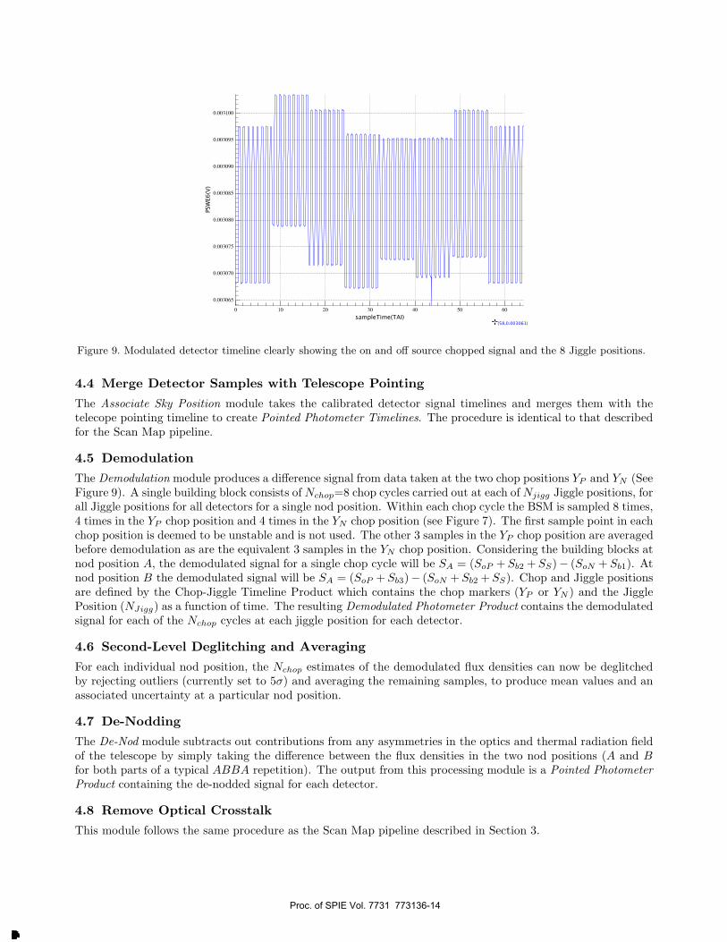
Figure 9. Modulated detector timeline clearly showing the on and off source chopped signal and the 8 Jiggle positions.

4.4 Merge Detector Samples with Telescope Pointing

The Associate Sky Position module takes the calibrated detector signal timelines and merges them with thetelecope pointing timeline to create Pointed Photometer Timelines. The procedure is identical to that describedfor the Scan Map pipeline.

4.5 Demodulation

The Demodulation module produces a difference signal from data taken at the two chop positions YP and YN (SeeFigure 9). A single building block consists of Nchop=8 chop cycles carried out at each of Njigg Jiggle positions, forall Jiggle positions for all detectors for a single nod position. Within each chop cycle the BSM is sampled 8 times,4 times in the YP chop position and 4 times in the YN chop position (see Figure 7). The first sample point in eachchop position is deemed to be unstable and is not used. The other 3 samples in the YP chop position are averagedbefore demodulation as are the equivalent 3 samples in the YN chop position. Considering the building blocks atnod position A, the demodulated signal for a single chop cycle will be SA = (SoP + Sb2 + SS)− (SoN + Sb1). Atnod position B the demodulated signal will be SA = (SoP + Sb3)− (SoN + Sb2 + SS). Chop and Jiggle positionsare defined by the Chop-Jiggle Timeline Product which contains the chop markers (YP or YN ) and the JigglePosition (NJigg) as a function of time. The resulting Demodulated Photometer Product contains the demodulatedsignal for each of the Nchop cycles at each jiggle position for each detector.

4.6 Second-Level Deglitching and Averaging

For each individual nod position, the Nchop estimates of the demodulated flux densities can now be deglitchedby rejecting outliers (currently set to 5σ) and averaging the remaining samples, to produce mean values and anassociated uncertainty at a particular nod position.

4.7 De-Nodding

The De-Nod module subtracts out contributions from any asymmetries in the optics and thermal radiation fieldof the telescope by simply taking the difference between the flux densities in the two nod positions (A and Bfor both parts of a typical ABBA repetition). The output from this processing module is a Pointed PhotometerProduct containing the de-nodded signal for each detector.

4.8 Remove Optical Crosstalk

This module follows the same procedure as the Scan Map pipeline described in Section 3.

Proc. of SPIE Vol. 7731 773136-14


4.9 Average Over Nod Cycles and the Level 1 Product

If there are more than a single ABBA nod cycle, the Average Nod Cycles module calculates a weighted mean anduncertainty from the separate estimates for each nod cycle. The Level 1 data product for the SPIRE Point Sourcepipeline is termed an Averaged Pointed Photometer Product (APPP) and contains the demodulated, de-noddedsignal at each of the 7 jiggle positions for every detector.

4.10 Fit Point Source Flux and Position and the Level 2 Product

For the seven-point jiggle there are eight data points for each detector (for each input APPP), one for eachspecific jiggle position. This distribution is fitted with a Gaussian approximation to the main beam profile toderive the source flux density and offset with respect to the pointed position. The estimation of flux density andposition are carried out independently. In addition, in the case of point source observations, three detectors ineach array see the source at some time during the observation: a primary, upper and lower detector set (SeeFigure 7, currently set to be PSW E6 (prime), E2, E10, PMW D8 (prime), D11, D5, PLW C4 (prime), C2, C6).The primary detector sees the source in both nod cycles; however, the other two detector sets only see the sourcein one of the nod positions. Thus, in the course of the observation, five different sky positions are viewed by thethree detectors (per array). Therefore it is expected that there will be a positive signal in the prime detector andnegative signals with half the amplitude in two others. The final Level 2 data product is the Jiggled PhotometerProduct which contains a single measurement of the flux and position of the target for each of the three detectorarrays taking into account all available data.

5. MAP CALIBRATION CONVENTIONS

The calibration convention for SPIRE Scan Maps and Jiggled Photometer Products is that the output fluxdensities are given in Jy per beam. This is discussed in some detail in the SPIRE Observers’ Manual, but wetouch on some of the key issues here.

Calibration in Jy/beam may be best explained by an example. Consider a 1 Jy point-like source (i.e., ofsize much smaller than the Herschel diffraction beam) at λ = 350 μm, and ignore random detector noise andinevitable calibration error. Except for a caveat regarding spectral slope (explained below), this source shouldproduce exactly a 1 Jy deflection in the Level 1 product for a PMW detector which is aligned perfectly with thepoint source. Except for a second caveat regarding map pixel size (also explained below), this same source shouldalso produce a 1 Jy peak signal in the Level 2 map in the case that the source position corresponds exactly withthe center of a map pixel.

Now, the caveat about map pixel size: The standard map maker bins the measurements, which have quasi-continuous positional information, into discrete, relatively coarse map pixels. A map pixel with center corre-sponding exactly to the point source position will collect some measurements with the reported flux densityequal to the true flux density. However, the pixel will also accumulate measurements where the source andmeasurement position are misaligned by up to 0.7 times the pixel width, and the reported flux density for thosemeasurements will be somewhat lower than the true flux density. This average reduction of the map signal iscalculated to be 5% to 7% for the default pixel scales.

A point source which does not align with the center of a map pixel will experience an additional reductionin the peak observed flux in the map. In this more general case, the true flux can be derived by fitting with themeasured beam shape. This is currently being studied by the ICC (with the preliminary result that photometrywith <1% precision is challenging), and a recommended method will be documented at a later date.

Regarding the caveat about spectral slope: The convention for SPIRE is that true flux densities at 250,350, or 500 μm are only equal to flux densities reported at the Level 2 stage when the source spectrum Sν isproportional to ν−1. Furthermore, the convention is to quote all flux densities at λ exactly equal to 250, 350,and 500 μm and to make color corrections for spectral slope, rather than to compute effective wavelengths. Thecolor corrections have been calculated using the measured Relative Spectral Response Functions (RSRFs), andare a few % for typical source spectra.

Proc. of SPIE Vol. 7731 773136-15


A resolved source with integrated flux equal to 1 Jy will, of course, produce a signal in the Level 1 and Level2 products which is less than 1 Jy/beam. Flux densities of extended sources can be measured by summing mappixels and dividing by the beam area:

S =L2

∑i Mi

Ωbeam, (6)

where S is the integrated flux, L2 is the area of a map pixel, M is the signal in a map pixel, and Ωbeam is thebeam area (tabulated in the SPIRE Observers’ Manual).

6. DATA HANDLING AND ARCHIVING

By design Herschel operates autonomously. The recorded data from Herschel observations are stored on-boardand transmitted to the ground station (either New Norcia, Australia or Cebreros, Spain) during the ∼3 hour ofdaily telecommunication periods.

The raw satellite, science, and housekeeping telemetry, received by the ground stations, is consolidated in theMission Operations Centre (MOC) in the European Space Operations Centre (ESOC) in Darmstadt, Germany.The fully consolidated data for a given observational day are then transmitted to the Herschel Science Centre(HSC) at the European Space Astronomy Centre (ESAC) near Madrid, Spain. The raw telemetry is ingestedin a special object-oriented database and a flag, indicating that the full consolidated telemetry packets andthe necessary auxiliary products (like the satellite attitude history file) are received, triggers automatic dataprocessing using the so-called Systematic Product Generation (SPG) with instrument pipelines developed in theHerschel Common Software System (HCSS).

The SPG pipelines process the data from each astronomical observing request to products at different levels,depending on the observing mode. Upon successful termination, the data are stored in the Herschel ScienceArchive (HSA). A quality assessment is performed by the HSC, and the principal investigator of the observingprogram is notified that his/her data are available for retrieval.

The HSA can be accessed via a standard web interface, common to most of the ESA missions (e.g., ISO, Inte-gral, XMM), as well as through HIPE. In general, the observations have a proprietary period of one year. Thereare some public data already available now: some Science Demonstration data as well as calibration observationsperformed with standard observing modes. Loading the data in HIPE allows for interactive processing of theobservations with the standard or with a modified version of the pipeline.

7. FUTURE DIRECTIONS

Within HIPE version 5, there will be a more versatile baseline removal tool available for users to run interactively.This tool allows a robust polynomial fit of a specified order with rejection of outliers. The user can select if thefit should be done on a scan-by-scan basis (memory efficient) or over the entire observation. The purpose of thisnew tool is to better estimate detector baselines in the presence of sources (Section 3.12).

First tests have shown that a higher order polynomial fit to the baseline of the whole observation is necessaryin many cases to successfully run madMap. The aforementioned task will provide this functionality and allowthe subsequent final validation of madMap.

An alternative approach to detector baseline subtraction is to use the cross-linked scans to determine therelative detector offsets at regions of overlap. This process implicitly uses the map of the sky and is easiest toimplement with an iterative approach.12, 13 The least-squares version of this iterative destriper minimizes:

χ2 =∑

b,i

(db,i − Cb − gbM(rb,i)

σb,i)2, (7)

where b is the bolometer index, i is the time index, d is the Level 1 detector sample, C is the detector offset,M is the flux density at position r in the map, and gb is an optional correction to the bolometer gain. C couldbe determined on an observation-by-observation or scanline-by-scanline basis. An iterative destriper is underevaluation and is planned for HIPE version 5.

Proc. of SPIE Vol. 7731 773136-16


Iterative mapping also facilitates second-level deglitching – rejection of outliers based on multiple measure-ments of the same map pixel – but this is not necessarily tied to the iterative destriper. The ICC will considerthe option of adding second-level deglitching in the processing between Levels 1 and 2 for later versions of HIPE.

We conclude by noting that the SPIRE photometer pipelines through HIPE version 3 that were used forScience Demonstration Phase have already produced high quality data. Calibration has moved part way frompre-flight estimates to in-flight measurements; with the imminent release of nonlinearity correction and absoluteflux calibration based on flight data and Neptune observations in HIPE version 4, we can expect further gains inaccuracy. Various other pipeline enhancements are anticipated in the next six to twelve months, allowing SPIREusers to extract the full capabilities of the instrument in their science data analyses.

ACKNOWLEDGMENTS

SPIRE has been developed by a consortium of institutes led by Cardiff Univ. (UK) and including Univ. Leth-bridge (Canada); NAOC (China); CEA, LAM (France); IFSI, Univ. Padua (Italy); IAC (Spain); StockholmObservatory (Sweden); Imperial College London, RAL, UCL-MSSL, UKATC, Univ. Sussex (UK); Caltech,JPL, NHSC, Univ. Colorado (USA). This development has been supported by national funding agencies: CSA(Canada); NAOC (China); CEA, CNES, CNRS (France); ASI (Italy); MCINN (Spain); SNSB (Sweden); STFC(UK); and NASA (USA). HCSS, HSpot, and HIPE are a joint development by the Herschel Science GroundSegment Consortium, consisting of ESA, the NASA Herschel Science Center, and the HIFI, PACS and SPIREconsortia.

We thank the SPIRE SAG2 for the permission to show their map of NGC 6822 and our commissioning phasemap of one of their objects (M83).

REFERENCES[1] Pilbratt, G. L., Riedinger, J. R., Passvogel, T., Crone, G., Doyle, D., Gageur, U., Heras, A. M., Jewell, C.,

Metcalfe, L., Ott, S., and Schmidt, M., “Herschel Space Observatory - An ESA facility for far-infrared andsubmillimetre astronomy,” ArXiv e-prints (May 2010).

[2] Griffin, M. J., Abergel, A., Abreu, A., Ade, P. A. R., Andre, P., Augueres, J., Babbedge, T., Bae, Y.,Baillie, T., Baluteau, J., Barlow, M. J., Bendo, G., Benielli, D., Bock, J. J., Bonhomme, P., Brisbin, D.,Brockley-Blatt, C., Caldwell, M., Cara, C., Castro-Rodriguez, N., Cerulli, R., Chanial, P., Chen, S., Clark,E., Clements, D. L., Clerc, L., Coker, J., Communal, D., Conversi, L., Cox, P., Crumb, D., Cunningham,C., Daly, F., Davis, G. R., De Antoni, P., Delderfield, J., Devin, N., Di Giorgio, A., Didschuns, I., Dohlen,K., Donati, M., Dowell, A., Dowell, C. D., Duband, L., Dumaye, L., Emery, R. J., Ferlet, M., Ferrand, D.,Fontignie, J., Fox, M., Franceschini, A., Frerking, M., Fulton, T., Garcia, J., Gastaud, R., Gear, W. K.,Glenn, J., Goizel, A., Griffin, D. K., Grundy, T., Guest, S., Guillemet, L., Hargrave, P. C., Harwit, M.,Hastings, P., Hatziminaoglou, E., Herman, M., Hinde, B., Hristov, V., Huang, M., Imhof, P., Isaak, K. J.,Israelsson, U., Ivison, R. J., Jennings, D., Kiernan, B., King, K. J., Lange, A. E., Latter, W., Laurent,G., Laurent, P., Leeks, S. J., Lellouch, E., Levenson, L., Li, B., Li, J., Lilienthal, J., Lim, T., Liu, J., Lu,N., Madden, S., Mainetti, G., Marliani, P., McKay, D., Mercier, K., Molinari, S., Morris, H., Moseley,H., Mulder, J., Mur, M., Naylor, D. A., Nguyen, H., O’Halloran, B., Oliver, S., Olofsson, G., Olofsson,H., Orfei, R., Page, M. J., Pain, I., Panuzzo, P., Papageorgiou, A., Parks, G., Parr-Burman, P., Pearce,A., Pearson, C., Perez-Fournon, I., Pinsard, F., Pisano, G., Podosek, J., Pohlen, M., Polehampton, E. T.,Pouliquen, D., Rigopoulou, D., Rizzo, D., Roseboom, I. G., Roussel, H., Rowan-Robinson, M., Rownd, B.,Saraceno, P., Sauvage, M., Savage, R., Savini, G., Sawyer, E., Scharmberg, C., Schmitt, D., Schneider,N., Schulz, B., Schwartz, A., Shafer, R., Shupe, D. L., Sibthorpe, B., Sidher, S., Smith, A., Smith, A. J.,Smith, D., Spencer, L., Stobie, B., Sudiwala, R., Sukhatme, K., Surace, C., Stevens, J. A., Swinyard, B. M.,Trichas, M., Tourette, T., Triou, H., Tseng, S., Tucker, C., Turner, A., Vaccari, M., Valtchanov, I., Vigroux,L., Virique, E., Voellmer, G., Walker, H., Ward, R., Waskett, T., Weilert, M., Wesson, R., White, G. J.,Whitehouse, N., Wilson, C. D., Winter, B., Woodcraft, A. L., Wright, G. S., Xu, C. K., Zavagno, A.,Zemcov, M., Zhang, L., and Zonca, E., “The Herschel-SPIRE instrument and its in-flight performance,”ArXiv e-prints (May 2010).

Proc. of SPIE Vol. 7731 773136-17


[3] Griffin, M., Dowell, C. D., Lim, T., Bendo, G., Bock, J., Cara, C., Castro-Rodriguez, N., Chanial, P.,Clements, D., Gastaud, R., Guest, S., Glenn, J., Hristov, V., King, K., Laurent, G., Lu, N., Mainetti,G., Morris, H., Nguyen, H., Panuzzo, P., Pearson, C., Pinsard, F., Pohlen, M., Polehampton, E., Rizzo,D., Schulz, B., Schwartz, A., Sibthorpe, B., Swinyard, B., Xu, K., and Zhang, L., “The Herschel-SPIREphotometer data processing pipeline,” in [Space Telescopes and Instrumentation 2008: Optical, Infrared,and Millimeter ], Proc. SPIE 7010 (Aug. 2008).

[4] Ott, S. in [Astronomical Data Analysis Software and Systems XIX ], Mizumoto, Y., Morita, K.-I., and Ohishi,M., eds., ASP Conference Series (2010).

[5] Kilbourne, C. A., Boyce, K. R., Brown, G. V., Cottam, J., Figueroa-Feliciano, E., Fujimoto, R., Furusho,T., Ishisaki, Y., Kelley, R. L., McCammon, D., Mitsuda, K., Morita, U., Porter, F. S., Ota, N., Saab,T., Takei, Y., and Yamamoto, M., “Analysis of the Suzaku/XRS background,” Nuclear Instruments andMethods in Physics Research A 559, 620–622 (Apr. 2006).

[6] Ordenovic, C., Surace, C., Torresani, B., Llebaria, A., and Baluteau, J. P., “Use of a local regularity analysisby a wavelet analysis for glitch detection,” in [Society of Photo-Optical Instrumentation Engineers (SPIE)Conference Series ], A. G. Tescher, ed., Proc. SPIE 5909, 556–567 (Aug. 2005).

[7] Swinyard, B. M., Ade, P., Baluteau, J., Aussel, H., Barlow, M. J., Bendo, G. J., Benielli, D., Bock, J.,Brisbin, D., Conley, A., Conversi, L., Dowell, A., Dowell, D., Ferlet, M., Fulton, T., Glenn, J., Glauser, A.,Griffin, D., Griffin, M., Guest, S., Imhof, P., Isaak, K., Jones, S., King, K., Leeks, S., Levenson, L., Lim,T. L., Lu, N., Makiwa, G., Naylor, D., Nguyen, H., Oliver, S., Panuzzo, P., Papageorgiou, A., Pearson,C., Pohlen, M., Polehampton, E., Pouliquen, D., Rigopoulou, D., Ronayette, S., Roussel, H., Rykala, A.,Savini, G., Schulz, B., Schwartz, A., Shupe, D., Sibthorpe, B., Sidher, S., Smith, A. J., Spencer, L., Trichas,M., Triou, H., Valtchanov, I., Wesson, R., Woodcraft, A., Xu, C. K., Zemcov, M., and Zhang, L., “In-flightcalibration of the Herschel-SPIRE instrument,” ArXiv e-prints (May 2010).

[8] Moreno, R., [These de Doctorat ], Universite de Paris VI (1998).[9] Moreno, R., [Neptune and Uranus planetary brightness temperature tabulation ], available frm ESA Herschel

Science Center (2010).[10] Schulz, B., Bock, J. J., Lu, N., Nguyen, H. T., Xu, C. K., Zhang, L., Dowell, C. D., Griffin, M. J.,

Laurent, G. T., Lim, T. L., and Swinyard, B. M., “Noise performance of the Herschel-SPIRE bolometersduring instrument ground tests,” in [Society of Photo-Optical Instrumentation Engineers (SPIE) ConferenceSeries ], Proc. SPIE 7020 (Aug. 2008).

[11] Cantalupo, C. M., Borrill, J. D., Jaffe, A. H., Kisner, T. S., and Stompor, R., “MADmap: A Massively Par-allel Maximum Likelihood Cosmic Microwave Background Map-maker,” Astrophysical Journal SupplementSeries 187, 212–227 (Mar. 2010).

[12] Bendo, G. J., Wilson, C. D., Pohlen, M., Sauvage, M., Auld, R., Baes, M., Barlow, M. J., Bock, J. J.,Boselli, A., Bradford, M., Buat, V., Castro-Rodriguez, N., Chanial, P., Charlot, S., Ciesla, L., Clements,D. L., Cooray, A., Cormier, D., Cortese, L., Davies, J. I., Dwek, E., Eales, S. A., Elbaz, D., Galametz, M.,Galliano, F., Gear, W. K., Glenn, J., Gomez, H. L., Griffin, M., Hony, S., Isaak, K. G., Levenson, L. R.,Lu, N., Madden, S., O’Halloran, B., Okumura, K., Oliver, S., Page, M. J., Panuzzo, P., Papageorgiou, A.,Parkin, T. J., Perez-Fournon, I., Rangwala, N., Rigby, E. E., Roussel, H., Rykala, A., Sacchi, N., Schulz,B., Schirm, M. R. P., Smith, M. W. L., Spinoglio, L., Stevens, J. A., Sundar, S., Symeonidis, M., Trichas,M., Vaccari, M., Vigroux, L., Wozniak, H., Wright, G. S., and Zeilinger, W. W., “The Herschel SpaceObservatory view of dust in M81,” ArXiv e-prints (May 2010).

[13] Levenson, L. R. and et al., “HerMES: Science Demonstration Phase Maps,” Monthly Noticies of the RoyalAstronomical Society , in preparation (2010).

Proc. of SPIE Vol. 7731 773136-18


Status of the SPIRE photometer data processing pipelines...

Documents

Transcript of Status of the SPIRE photometer data processing pipelines...