Status and Trends of Wetlands in the Long Island Sound ...
37
Picture paint Status and Trends of Wetlands in the Long Island Sound Area: 130 Year Assessment U.S. Fish & Wildlife Service
Transcript of Status and Trends of Wetlands in the Long Island Sound ...
Picture
paint
Status and Trends of Wetlands
in the Long Island Sound Area:
130 Year Assessment
Status and Trends of Wetlands in the Long Island Sound Area:
130 Year Assessment
U.S. Fish & Wildlife Service
U.S. Fish & Wildlife Service

2
Georgia Basso U.S. Fish and Wildlife Service Kevin O’Brien CT Department of Energy and Environmental Protection Melissa Albino Hegeman and Victoria O’Neill NY State Department of Environmental Conservation

3
Acknowledgements
The authors would like to recognize the contributions of the following key individuals who
supported the completion and review of this study: Mark Tedesco (U.S. Environmental
Protection Agency) and Dawn McReynolds (New York State Department of Environmental
Conservation).
Review of the study findings and report was provided by the following subject material experts:
Susan Adamowicz (U.S. Fish and Wildlife Service), Maureen Correll (The University of Maine),
Chris Elphick (University of Connecticut), Charles Frost (U.S. Fish and Wildlife Service), Letitia
Grenier (San Francisco Estuary Institute), Troy Hill (Yale School of Forestry & Environmental
Studies), Nicole Maher (The Nature Conservancy), Ralph Tiner (U.S. Fish and Wildlife Service),
Suzanne Paton (U.S. Fish and Wildlife Service), Cathleen Wigand (U.S. Environmental
Protection Agency) and Elizabeth Watson (Academy of Natural Sciences of Drexel University).
Reference material support was provided by Rebecca Garvin (U.S. Environmental Protection
Agency) and Ana Herrera (U.S. Environmental Protection Agency).
This work was partially funded by the interagency agreement between the U.S. Environmental
Protection Agency and the U.S. Fish and Wildlife Service.
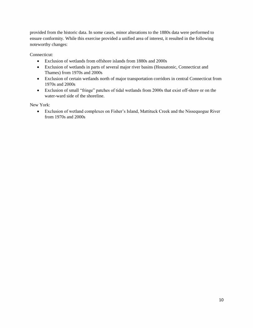
Front cover photo: Barn Island Wildlife Management Area, Stonington, CT. Charlotte
Murtishaw (USFWS).
Inside cover photo: Barn Island Wildlife Management Area, Stonington, CT. Charlotte
Murtishaw (USFWS).
This report should be cited as:
G. Basso, K. O’Brien, M. Albino Hegeman and V. O’Neill. 2015. Status and trends of wetlands in the Long
Island Sound Area: 130 year assessment. U.S. Department of the Interior, Fish and Wildlife Service. (36 p.)

4
Table of Contents
Abstract ......................................................................................................................................................... 6
Introduction ................................................................................................................................................... 6
Value of Tidal Wetlands ........................................................................................................................... 6
The Importance of a Historic Perspective ................................................................................................. 7
Methods ........................................................................................................................................................ 8
Establishing a Common Area of Interest: ................................................................................................. 9
Assessing Wetland Components: ............................................................................................................ 12
Open Water Assessment ......................................................................................................................... 14
Results – Wetland Change .......................................................................................................................... 15
Wetland Change Error Estimates – Providing upper and lower boundary estimates ............................. 16
Discussion ................................................................................................................................................... 17
Causes of Marsh Loss- Historic and Present Day ................................................................................... 17
Other Local Studies: A Summary ........................................................................................................... 20
Loss of Ecosystem Services .................................................................................................................... 22
Recommendations for the Long Island Sound Area .............................................................................. 23
Literature Cited ........................................................................................................................................... 26
Appendix ..................................................................................................................................................... 31
Acronyms .................................................................................................................................................. 5
Error Estimates........................................................................................................................................ 31
Data Source Descriptions ........................................................................................................................ 35
5
List of Tables
Table 1. Data sources for historic, intermediate and present day estimates of wetlands .............................. 9
Table 2. Total acreage values for original source data (unaltered) ............................................................... 9
Table 3. Prominent wetland components included and excluded from 1970 and 2000 era data ................ 14
Table 4. Revised tidal wetland acreages spatially reduced to the common footprint ................................. 14
Table 5. Tidal wetland open water assessment: Indicators, metrics and cut points .................................... 15
Table 6. Estimated percentage change in wetland acres in the Long Island Sound area ............................ 16
Table 7. Open water scores by basin and overall habitat quality score ...................................................... 16
List of Figures
Figure 1. Long Island Sound Study coastal boundary .................................................................................. 8
Figure 2. Footprint of 1880s and 1970s New York and Connecticut data sets ........................................... 11
Figure 3. T-Sheet image from Connecticut. ................................................................................................ 12
Figure 4. Example of 1970s and 2000s wetland data for Connecticut.. ...................................................... 12
Figure 5. 2000 era NWI tidal wetlands, unconsolidated bottoms and 1970 era boundary in Connecticut . 13
Figure 6. Infrared and true color photos of open water assessment ............................................................ 18
Figure 7. Saltmarsh sparrow nest ................................................................................................................ 19
Figure 8. Marsh elevations Connecticut and New York. ............................................................................ 20
Figure 9. Average annual wetland change estimates for the conterminous U.S., 1954 to 2009 ................. 22
Figure 10. Ecosystem service loss estimates in the Long Island Sound.. ................................................... 23
Acronyms
CT DEEP Connecticut Department of Energy and Environmental Protection
EPA U.S. Environmental Protection Agency
GIS Geographic Information System
LIS Long Island Sound
LISS Long Island Sound Study NOAA National Oceanic and Atmospheric Administration
NWI National Wetlands Inventory
NYSDEC New York State Department of Environmental Conservation
T-Sheets Topographic Survey Sheets
USFWS U.S. Fish and Wildlife Service

6
Abstract
This report provides the first 130 year assessment of tidal wetland change for the entire Long Island
Sound area. The results indicate an overall 31% loss of tidal wetlands with a 27% loss in Connecticut and
48% loss in New York. Despite tidal wetland legislation passed in the 1970s, wetland decline in Long
Island Sound continues. After the 1970s New York sustained more wetland loss (a decrease of 19%) than
Connecticut (a slight gain of 8%). Current research points to multiple, nuanced and complex causes of
present-day tidal wetland changes. A major present-day concern is wetland vulnerability to loss due to
potentially increased amounts of open water on the marsh surface. An open water assessment initially
conducted in Connecticut indicates an average of 47% permanent open water on the marshes studied – a
less healthy status. Understanding the extent and context of tidal wetland change is important for effective
future protection. In addition to overall loss, we discuss the historic extent, present-day stressors and
importance and implications of wetland decline to the Long Island Sound ecosystem. We summarize
other local studies of marsh decline and degradation in portions of the Long Island Sound and conclude
with recommendations for protecting this valuable habitat type given historical context and current
stressors.
Introduction
Value of Tidal Wetlands
Tidal wetlands are among the most valuable of the earth’s habitats from an ecosystem service perspective
(Gedan 2009, Costanza 1997). They provide spawning, nursery and feeding grounds to resident and
migratory marine organisms including shellfish, finfish and waterfowl; they play an important role in
nutrient cycling within estuaries (Teal 1986, Mitsch 1993, Dahl 2013) and they provide services to people
including storm protection, water purification, erosion control, nutrient sequestration and nursery habitat
for fish (Weber 2014, Tiner 2013, Gedan 2009, Barbier 2011).
Tidal wetlands play a particularly important role in nitrogen removal. Wetland vegetation slows water
current and removes sediment and other pollutants including excess nitrogen. The nitrogen is deposited in
the sediment or taken up by the plants. This improves water quality, stabilizes shorelines and prevents
erosion and flooding (Teal 1986, Mitsch 1993).
Tidal wetlands also play a critical role in carbon sequestration. More than half of the global carbon load is
captured by marine ecosystems and coastal vegetation. This carbon is known collectively as "blue
carbon." The top three blue carbon sinks are mangroves, seagrass and tidal wetlands (Nellemann 2009).
These habitats not only remove more carbon than all other ocean habitat types but they remove it at rates
up to 100 times faster than terrestrial forests (Nellemann 2009, The Blue Carbon Project 2014). Salt
marshes have the highest average carbon burial rate per hectare per year of all the blue carbon sinks
(Nellemann 2009) and, although they cover a relatively small area, carbon burial by salt marshes accounts
for an estimated 21% of the total carbon sink of all ecosystems in the United States (Bridgham 2006).
Tidal wetlands are a high-value habitat from multiple perspectives. Kocian (2014) estimated the economic
value of the Long Island Sound area using benefits transfer methodology. Kocian concludes that coastal
wetlands provide the highest monetary value of all the land cover types assessed in the Long Island Sound

7
area, with an estimated range of $11,699 to $77,260 per acre per year (2014 values). This calculated value
includes food, storm protection, wastewater treatment, habitat, nursery, recreation and tourism benefits.
Despite major restoration efforts and the immense value wetlands provide, marsh degradation due to
human activity is extensive and increasing (Barbier 2011, Palmer 2008). To date, humans have damaged
or destroyed about 50% of wetlands globally (Barbier 2011). Current threats include hydrologic
modification, pollution, climate change, invasive species, herbivory and sediment deprivation (Silliman
2009, Kirwin 2013). Although significant, these threats do not doom wetlands to a trajectory of continued
degradation. Humans can begin to change this trajectory and in fact have begun to do so successfully in
some areas. Tampa Bay and San Francisco Bay as well as other estuaries across the country provide
examples of communities coming together to make meaningful changes that allow for tidal wetland
recovery.
The Importance of a Historic Perspective
Tidal wetlands are both extremely vulnerable and valuable to humans (Gedan 2009). Their continued
decline has an impact on people and ecosystems (Nellemann 2009, Lotze 2006, Craft 2009). An
understanding of historic reference points, as well as the extent of and reasons for degradation, is critical
to the success of large-scale restoration efforts (Lotze 2006). Historic information is valuable for goal
setting (Shumchenia 2015, Rosenberg 2005), helps prevent shifting ecological baselines (Rosenberg
2005) and allows for comparison across estuaries (Cicchetti and Greening 2011). Historic information
provides perspective on the magnitude and impact of wetland loss (Lotze 2006) and can be applied to
galvanize public support and spur further investigation into effective means of habitat protection
(Cicchetti and Greening 2011).
Work conducted under the Tampa Bay National Estuary Program and the San Francisco Bay Area
Wetlands Ecosystem Goals Project provide strong examples of how a historic perspective can be used to
set goals, establish context, galvanize public support and advance meaningful restoration. In the case of
Tampa Bay, managers used a historic context to frame initial habitat management discussions among
partners. A common vision for ecological health arose out of these conversations. This vision was turned
into quantifiable goals for a more ecologically desirable state of habitats in Tampa Bay (Cicchetti and
Greening 2011). Understanding extent and consequences of loss can give higher weight to protecting
what remains. This approach has been used in Tampa Bay to champion a collective goal to “hold the line”
in terms of extent and function while moving toward a more ecologically desired state (Cicchetti and
Greening 2011).
In the case of San Francisco Bay, managers and scientists calculated historic extent lost (Goals Project
1999) and used this historical context to estimate habitat acreage necessary to restore the ecological
integrity of estuarine wetlands in the region. They used the scientific recommendations resulting from this
large, collaborative effort to reset assumptions about the scale of restoration needed, galvanize political
support for increased funding and remove barriers to progress that stemmed from disagreements about
trade-offs among habitat types. Spurred by the Goals Project vision, wetland restoration leapt forward on
a much larger scale, even in this highly urbanized estuary (Goals Project 2015).

8
In addition to providing a sense of the magnitude of loss, historic information can also help frame future
change in a long-term context. This can broaden managers’ perspectives, encouraging a shift away from
narrow goals (i.e. restore 200 acres), which in isolation can seem large, to a more holistic, ecosystem
context (Rosenberg 2005).
While it may not be possible or even advisable to return to a historic condition (Duarte 2009), it is within
our reach to regain and protect the suite of values wetlands provide to people and the environment (Lotze
2006). With the understanding of a broad historic context, Lotze (2006) encourages “regeneration” and
restoration of the function provided by a network of coastal habitats so that they are able to absorb future
disasters and shocks. Palmer (2009) suggests moving a degraded system toward a more ecologically
desired state relative to a less disturbed time. By drawing on examples from other National Estuary
Programs, applying the historic findings in this report and the results from studies on current stressors we
can begin to identify and move toward a more desired state within the Long Island Sound area.
Methods
Wetland Change
This assessment was conducted on wetlands within the Long Island Sound Study (LISS) area coastal
boundary (Figure 1). Long Island Sound is an estuarine water body of approximately 1,300 square miles
located between the Connecticut shoreline and the north shore of Long Island, New York. Long Island
Sound is one of 28 National
Estuaries designated by the U.S.
Environmental Protection Agency
(EPA) across the country. The
Long Island Sound Study coastal
boundary delineates the terrestrial
and aquatic habitats that are within
the Long Island Sound area as per
the National Estuary designation.
Wetland data was compiled from
the late 19th century, the early
1970s and early 2000s from the
best available sources. These are
summarized in Table 1 and
described in greater detail in the
Appendix.
Figure 1. Red outline of the Long Island Sound Study coastal boundary.

9
Table 1. Data sources for historic, intermediate and present day estimates of wetlands.
Year(s) Connecticut Data Sources New York Data Sources
1880s National Oceanic and Atmospheric
Administration (NOAA) Topographic
Survey Sheets (T-Sheets), 1880 – 1890s
NOAA Topographic Survey Sheets (T-
Sheets), 1880 – 1890s
1970s Connecticut Department of Energy and
Environmental Protection (CT DEEP)
1970s Tidal Wetlands
New York State Department of
Environmental Conservation (NYSDEC)
1974 Tidal Wetlands Map
2000s National Wetlands Inventory (NWI)
2010-2012
National Wetlands Inventory (NWI)
2004-2009
A critical first step in this study was to systematically understand and, where needed, standardize how
wetland data was presented. By doing so, acreage estimates could be calculated from each of the years
(1880s, 1970s and 2000s) to get a reasonable comparison of the amount of total acres gained or lost.
Using multiple data sources presented a challenge. It was important to ensure that values calculated and
analyzed represented true change as consistently as possible. Simply using acreage totals from the various
data sets (Table 2) could under or over represent change if the data did not exist within the same or
similar geographic extents or if the data included or omitted certain features. Further, assessing a rough
magnitude of error was desirable to frame the results within a reasonable range of values rather than
simply providing one calculation (see Appendix). In some cases, data collection and challenges were
similar for both states. In other cases, due to differences in historic data and methodology, data was dealt
with on a state by state basis in order to make it as comparable as possible between states.
Table 2. Total acreage values for original source data (unaltered).
1880s 1970s 2000s
CT 20,075 16,765 17,206
NY 5,418 4,014 3,354
LIS Total 25,493 20,779 20,560
Establishing a Common Area of Interest
Overlaying the spatial data immediately identified a primary problem in conflicting extents. Figure 2
presents some examples. The wetlands collected from the National Oceanic and Atmospheric
Administration (NOAA) Topographic Survey Sheets (T-Sheets) were constrained to the extent of the
mapping strategy and the available maps. Confidence is high that all available maps from the given time
period were collected and processed; however, the intent of the mapping itself was not to universally
capture all areas of Connecticut and New York or even all areas of coastal Connecticut and New York.
Rather, the intent of the T-sheets was primarily to capture the shoreline and the general vicinity thereof as
seen in Figure 3. So while there is much benefit to using this data, it cannot be construed to account for all
areas of wetlands during the late 19th century.
Therefore, the extent of the 1970s and 2000s era data in both Connecticut and New York was spatially
reduced by deleting or editing the boundaries of wetlands to create a spatially similar extent to that
10
provided from the historic data. In some cases, minor alterations to the 1880s data were performed to
ensure conformity. While this exercise provided a unified area of interest, it resulted in the following
noteworthy changes:
Connecticut:
Exclusion of wetlands from offshore islands from 1880s and 2000s
Exclusion of wetlands in parts of several major river basins (Housatonic, Connecticut and
Thames) from 1970s and 2000s
Exclusion of certain wetlands north of major transportation corridors in central Connecticut from
1970s and 2000s
Exclusion of small “fringe” patches of tidal wetlands from 2000s that exist off-shore or on the
water-ward side of the shoreline.
New York:
Exclusion of wetland complexes on Fisher’s Island, Mattituck Creek and the Nissequogue River
from 1970s and 2000s
11
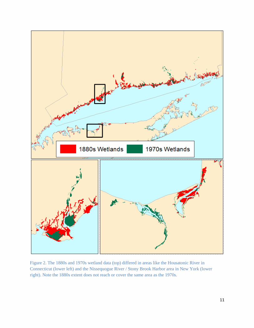
Figure 2. The 1880s and 1970s wetland data (top) differed in areas like the Housatonic River in
Connecticut (lower left) and the Nissequogue River / Stony Brook Harbor area in New York (lower
right). Note the 1880s extent does not reach or cover the same area as the 1970s.

12
Figure 3. A sample T-Sheet image from Connecticut with wetlands delineated in green. Note the limit of
the data captured is generally constrained to the shoreline.
Assessing Wetland Components
In Connecticut, the 1970s data is known to have excluded wetlands on offshore islands and certain areas
were omitted or missed. Further, wetland sites were not classified beyond labeling areas as ‘wetland.’
That is, there was no demarcation between any areas of internal landform features such as low marsh,
high marsh or hydrographic features (e.g. rivers, streams or ditches). In Figure 4 the purple boundary
defines the extent of a 1970 Connecticut wetland polygon on top of recent aerial photography showing
landform and hydrographic features that were included in the calculation of marsh area.
Figure 4. Example of 1970s (left) and 2000s (right) wetland data for Connecticut; note the inclusion of
hydrographic features as part of the 1970s polygon (left) and the exclusion of hydrographic features in the
2000 era NWI emergent tidal wetland data (right, only green area is counted).

13
The 2000 era NWI data for Connecticut provides information to extract the extent and classification of
emergent, forested and scrub-shrub tidal wetland areas in both brackish and freshwater regimes. When
compared to the 1970 era data, however, simply looking at these acreage values would suggest less area
in the 2000s, as the hydrographic features are included in marsh area in the 1970s and excluded from
marsh area in the 2000s (Figure 4). To some degree this issue also affects the 1880s wetlands data for
Connecticut; while it is technically feasible to fill in these gaps, it was beyond the scope of this
assessment. Fortunately, NWI also includes areas of unconsolidated bottom that are generally analogous
to the internal hydrographic features noted above. This allows a feasible way to provide a comparable
estimate of change by including both areas of wetland proper as well as unconsolidated bottom in the
2000 era NWI data. The unconsolidated bottoms were extracted from the 2000 era NWI data using the
1970s boundary and combined with the NWI wetland areas to best approximate the same relative extents
of wetland areas for comparison (Figure 5). Note that only unconsolidated bottoms were clipped from the
2000 era NWI data – the upland extents of emergent wetlands remain as-is. New York data did not have
this issue and no adjustment for hydrographic feature was necessary.
The New York 2000 era NWI data did indicate some
areas where known wetlands were not included in the
correct categories. Review of the data sets by
resource managers from the New York State
Department of Environmental Conservation
(NYSDEC) found that small, patchy, fringing
wetlands were sometimes lumped in with the
Unconsolidated Shore category. These wetlands were
too small to be mapped in their own right, but they
were still visible from aerial photos. In the case of
Oyster Bay Harbor, NY there were approximately 30
acres of Unconsolidated Shoreline that also
contained small amounts of wetlands. Oyster Bay
Harbor was the only complex in New York that
seemed to show any certain quantifiable acreage
mislabeled in this way. The approximate 30 acres
found in Oyster Bay Harbor were not included in the
analysis.
In contrast to the 1970 era Connecticut data, the 1970 era New York wetland data provides a series of
wetland categories. The intertidal marsh (IM), high marsh (HM) and fresh marsh (FM) categories were
included as vegetated marsh for this assessment. The total acreage from these categories, plus the acreage
from the formerly connected (FC) and dredge spoils (DS) make up the total New York 1970 era acreage.
The categories FC and DS pose a potential source of error because it is not possible to determine whether
these two categories were actually vegetated wetlands or not. The 2000 era vegetated tidal wetland
acreage included the categories from the NWI with a class equal to “Estuarine and Marine Wetland,” a
category that most closely resembled vegetated wetland categories mapped in the 1970s.
Table 3 summarizes how wetlands from 1970 and 2000 era data sets were synthesized in this study.
Figure 5. 2000 era NWI emergent tidal
wetlands (green), unconsolidated bottoms
(brown) and 1970 era wetland boundary
(purple) in Connecticut.

14
Table 3. Prominent wetland components included and excluded from 1970 and 2000 era data.
New York- 1970s Connecticut- 1970s
Included in acreage
estimate
Excluded Included in acreage
estimate
Excluded
FC (Formerly Connected) SM (Coastal Shoals and
Mud Flats)
“Wetland” (includes areas of
stream/river channels and
ditches)
The dataset systemically
excluded wetlands on
offshore (were not
surveyed) and
intermittently excluded
various wetlands.
DS (Dredge Spoils) Unconsolidated bottom
IM (Intertidal Marsh) LZ (Littoral Zone)
HM (High Marsh) AA(Adjacent Area)
FM (Fresh Marsh)
New York- 2000s Connecticut- 2000s
Included in acreage
estimate
Excluded Included in acreage
estimate
Excluded
Estuarine Emergent
(which encompassed IM,
HM, FM, DS, FC)
Unconsolidated bottom Estuarine Emergent brackish
and tidal wetlands (see table
X for full listing of NWI
codes”)
NWI features not
encompassing brackish or
freshwater tidal wetlands
(e.g. freshwater non-tidal
wetlands, unconsolidated
shores, flats, etc.
Unconsolidated shore
(which is very similar to
SM coastal shoals &
mudflats in 1974)
Unconsolidated bottom (AB-
US-UB-SB = aquatic bed,
unconsolidated shore,
bottom, stream) (Table 1)
NWI data on offshore
islands and waterward of
the shoreline.
AA & LZ don’t show up
in 2000 era NWI data
Table 4 provides revised acreage values for Connecticut and New York as a result of the establishment of
a common footprint.
Table 4. Revised tidal wetland acreages spatially reduced to the common footprint.
1880s 1970s 2000s
CT 19,828 13,443 14,566
NY 5,342 3,464 2,790
LIS Total 25,170 16,907 17,356
Open Water Assessment
In addition to an acreage change assessment, a habitat quality assessment was conducted with respect to
permanent open water (not tidal or rainfall) on the tidal marshes in Connecticut. Long Island Sound has
typically been divided into three geographic basins; Western, Central and Eastern (Koppelman et al.
1976). Permanent open water was assessed by basin.
Open water is considered an important indicator as wetlands are getting wetter, resulting in a loss of
vegetated marsh in Connecticut (Tiner 2013). Using 2010 Tide Controlled Coastal Infrared Aerial

15
Photography (Figure 6) coupled with field surveys, 25% of tidal wetland units greater than 10 acres in
each of the three Long Island Sound Study basins were randomly sampled. A team of wetlands experts
conducted photo interpretation of open water surface area and followed up with field checks to verify
surface conditions. The team visited 16 out of the 37 marshes included in the study and took an average of
23 point readings per marsh.
Cut points for extent of open water on the marsh were set based on input from wetland experts (Table 5).
The cut points delineate a specific numeric range for ‘poor’ ‘fair’ ‘good’ and ‘very good’ conditions. In
addition to input from wetland experts, the numeric range associated with each cut point was also
informed by recommendations developed for New England marshes (Adamowicz 2005). The "very good"
indicator aligns with Adamowicz (2005) finding that the average amount of open water in an unditched
New England marsh is 9% or 913 m2/ha.
Table 5. Tidal wetland open water assessment: Indicators, metrics and cut points.
Habitat Indicator Metric Cut Points
Poor Fair Good Very
Good
Tidal wetlands % open water
low tide
Total pool surface area per
hec (m2 of pool/ha salt
marsh)
> 20% 16 to
20%
10 to
15%
0 to 9%
Results – Wetland Change
Table 6 presents a synthesis of the results. Between the 1880s and 2000s there was an estimated 31% loss
in tidal wetland acreage (approximately 7,841 acres) within the Long Island Sound Study coastal
boundary. The majority of this loss occurred before 1970 with a 35% loss in New York and a 32% loss in
Connecticut.
Between 1970 and today loss in Connecticut slowed significantly. The data shows a small wetland gain
(8%). Wetland loss in New York continued over that same time period with a 19% loss in acreage
between the 1970s and 2000s.
In summary, both states lost a substantial percentage of wetland acreage between the 1880s and today,
with New York losing an estimated 48% of its wetland acres and Connecticut losing 27% of its wetland
acres. The subsequent section on error estimates provides a conservative range of values to frame upper
and lower bounds among the geographies and timeframes.

16
Table 6. Estimated percentage change in wetland acres in the Long Island Sound area.
1880s-1970s 1970s-2000s 1880s-2000s
Change
(Acres)
Change
(%)
Change
(Acres)
Change
(%)
Change
(Acres)
Change
(%)
CT -6,385 -32% 1,123 8% -5,262 -27%
NY -1,878 -35% -674 -19% -2,552 -48%
LIS
Total -8,263 -33% 449 3% -7,814 -31%
Results – Open Water Assessment
Marshes in the Connecticut sample study had an average of 46% permanent open water at low tide (total
pool surface area/ hectare of salt marsh). Open water within each of the basins was above 20% (Table 7),
putting all basins well within the poor range (Table 5).
Table 7. Open water scores by basin and overall habitat quality score.
Basin Tidal wetland
acres
Open water
acres
% open water
at low tide
Western 345 113 33%
Central 1,394 684 49%
Eastern 2,821 1,628 58%
Wetland Change Error Estimates – Providing upper and lower boundary estimates
Given the diversity of time and sources of data included in this analysis, it is appropriate to quantify some
of the uncertainties and possible sources of error to provide a meaningful way to frame change.
Shoreline change analyses that use data of similar vein and vintage can provide a reasonable way to
address this issue. Uncertainties for shorelines include errors introduced by data sources as well as errors
introduced by measurement methods and are well documented (Anders 1991, Crowell 1991, Thieler
1994, Moore 2000, Ruggiero 2003). Here, we assume that the errors associated from delineating and
mapping shorelines is more or less analogous to those applicable to creating wetland maps. Further the
methodologies used to define shoreline error bounds in Taylor (1997) and Hapke (2010) can also be used
to define wetland error bounds. A more detailed presentation on the adaption and implementation of the
methods can be found in the Appendix. The results include the following:
For Connecticut:
o Data from the 1880s to the 1970s indicated that the computed change could
conservatively vary between -40% and -18%.
o Data from the 1970s to the 2000s indicated that the computed change could
conservatively vary between +6% to +11%.
o Data from the 1880s to the 2000s indicated that the computed change could
conservatively vary between -37% to -9%
For New York:
o Data from the 1880s to the 1970s indicated that the computed change could
conservatively vary between -40% and -33%.

17
o Data from the 1970s to the 2000s indicated that the computed change could
conservatively vary between -31% to + 9%.
o Data from the 1880s to the 2000s indicated that the computed change could
conservatively vary between -54% to -35%.
For the entire LIS coastal boundary:
o Data from the 1880s to the 1970s indicated that the computed change could
conservatively vary between -39% and -22%.
o Data from the 1970s to the 2000s indicated that the computed change could
conservatively vary between -3% to +11%.
o Data from the 1880s to the 2000s indicated that the computed change could
conservatively vary between -40% to -14%.
Discussion
Given their importance to humans and wildlife, historic and present day marsh loss is a concern. This
assessment indicates that historically (between the 1880s and 1970s) Connecticut and New York
experienced a similar rate of decline (32% and 35% respectively). Post 1970s, loss in Connecticut may
have slowed or stopped (8% gain) while loss in New York continued (19% loss). The small gain in
Connecticut could be attributed to restoration acres, differences in how NWI classified land cover types,
the way the 1970 data was developed (see Appendix for brief description of the compilation
methodology) or some combination of all three. Overall between the 1880s and 2000s Long Island Sound
experienced a 31% decline in wetland acres, with Connecticut having lost 27% of its wetland acres and
New York having lost 48% of its wetland acres (Table 6). The 1880s serve simply as a point in time.
Wetlands were not in pristine condition at this time so the loss estimated in this report would most likely
be greater if an earlier point in time were selected. It should further be noted that this study did not look at
shifts in vegetative species. Vegetative shifts may be a more sensitive way of calculating wetland loss.
Wetland loss reduces the system's overall resilience, compromises ecosystem services like flood
protection and carbon sequestration and can have a negative impact on biological diversity (Wigand 2014,
Field 2014). In addition to wetland acreage loss in the LIS coastal boundary, salt marshes randomly
sampled in the open water assessment in Connecticut had high amounts of permanent open water on their
surface (on average 46% total pool surface area/ hectare of salt marsh). The amount of permanent open
water on marshes at low tide is a growing concern both locally and globally (Rozsa 1995, USFWS 2011).
Causes of Marsh Loss- Historic and Present Day
Some of the more substantial causes of loss before 1970 included dredge and fill operations (Rozsa 1995,
Tiner 2012). By in large, this form of wetland destruction stopped in both states with the passage of tidal
wetland acts in the 1970s (DEEP 2014, Tiner 2006, Rozsa 1995, Kirwan 2013). However, despite the
legislation and restrictions, anthropogenic stresses continue to impact wetlands, resulting in loss within
the LIS area (Mushacke 1999, Mushacke 2007). Although there is debate about which stressors are the
main drivers of wetland decline and how they vary based on location; major stressors generally include
nutrients, invasive species, sediment deprivation, hydraulic modification, pollution and climate change
(Smith 2009, Gedan 2009, Wigand 2014, Watson 2014, Silliman 2009, Kirwan 2013). All are the result

18
of human activities (Silliman 2009) and can act synergistically to deteriorate wetlands (Silliman 2009,
Lotze 2006).
In contrast to the dredge and fill days of the past, the main cause of marsh loss in developed countries
today is unintentional conversion of wetlands to open water (Kirwan 2013). Reasons for this conversion
are complex and may include a combination of stressors. Irrespective of the causes, a growing body of
research highlights instances and places where marshes are wetter and vegetated areas are shifting from
high marsh to low marsh or to mud flat both locally and globally (Warren and Niering 1993, Muschacke
2007, Tiner 2006, Field 2014, Rozsa 1995, Watson et al. 2014, Smith 2009, USFWS 2011). Current
research indicates that marsh transgression may not be happening quickly or consistently enough to
prevent loss of high marsh (Field 2014).
Tiner 2006 examined several wetland complexes in western Connecticut and found that all study areas
experienced a decline in low marsh from 1974 to 2004 and a gain in tidal flats. All areas, except Cos Cob
Harbor in Greenwich, CT, also experienced a loss in high marsh. This type of wetland loss may be
indicative of a regime shift. As described by Folke (2004), a regime shift is characterized by a shift from
one ecosystem to another, often resulting in considerably less service and benefit to humans. It can be a
difficult process to reverse (Folke 2004). Rozsa (1995) noted that on Connecticut’s western shore large
areas of marsh in Norwalk and on the Five Mile River have drowned. Warren and Niering (1993) note
areas of high marsh in Southern New England that have transitioned to S. alterniflora, a plant species
characteristic of low marsh. Field (2014) notes that high elevation marsh species (Juncus gerardii) are
disappearing and lower elevation species (Spartinia alterniflora) are increasing. Muschacke (2007) did
not attribute wetland loss in New York to a single cause but suspected sea level rise to be the primary
driver of losses observed between 1974 and 2006. He noted that some complexes along Long Island
Sound, like Crab Meadow in Northport NY, exhibited a vegetative regime shift, where high marsh had
shifted to low marsh. Muschacke surmised this conversion was the result of higher tides and greater
flooding inundation. In our initial assessment we found that on average the marshes studied had well over
20% open water (Table 7), which is more water than is conducive to a functioning, healthy New England
salt marsh (Adamowicz 2005). This water is permanent open water and not pannes, pools, tidal or rainfall
(Figure 6). The amount of water on many salt marshes in Connecticut indicates that they may be close to
if not past a tipping point or regime shift (S. Adamowicz, pers. comm.). It should be noted that in 2010
the metonic cycle, a 19 year lunar cycle that affects the tides, was high. This may contribute to more open
water on the marsh surface during this time
period.
Figure 6. Infrared and true color photos of ‘very
good’ (top, Hammonasset State Park, Madison)
and ‘poor’ (bottom, Leetes Island, Guilford)
marshes surveyed along the Connecticut coast.

19
The work summarized above, specific to the LIS area, also aligns with national trends. The most recent
report from the USFWS on the status of our nation’s wetlands concludes that 83% of wetland loss
between 2004 and 2009 was due to salt water intrusion and conversion to open water (USFWS 2011).
Wetter marshes pose a problem for the integrity of the marsh and the species that rely on them. In their
2014 study, Field et al found that Willet, Clapper Rail, Seaside Sparrow and Saltmarsh Sparrow
populations in occupied salt marshes are declining on the Connecticut Coast. The amount of decline
experienced by these four salt marsh obligate salt marsh species is consistent with what would be
expected if sea level rise was the cause, with an inverse correlation between nest elevation and species
decline whereby species nesting at the lowest elevation experience the steepest decline (C. Elphick, pers.
comm.). Of the four species listed above, the Saltmarsh Sparrow nests at the lowest elevation. Saltmarsh
Sparrow nest density has declined over the past ten years. The biggest cause of nest failure is
flooding during especially high tides, which results in egg losses and nestlings drowning (Figure 7).
Figure 7. Salt water intrusion likely threatens
the future survival of Saltmarsh Sparrows.
Photo credit: Jeanna Mielcarek, UCONN
Systematic Heath Action Research Program
(SHARP).
The results of this assessment indicate that post-1970 marsh acreage losses are more substantial in New
York than Connecticut. Accelerated loss in New York as compared to Connecticut may be due in part to
differences in elevation and suspended solid loads between the two states. Connecticut marshes appear to
be higher in elevation than many marshes on Long Island (Figure 8, Watson et al. 2014). Watson looked
at eight marshes in Rhode Island and New York and found that marshes at lower elevations experienced
higher rates of vegetation loss (1970-2010) whereas higher elevation marshes had greater resilience.
Marshes at a lower elevation are more vulnerable to conversion to mud flat than those at higher elevations
due to sea level rise (Wigand 2014, Watson 2014). However, tidal range in Long Island Sound varies and
marsh elevations approximate the height of mean high water (McKee and Patrick 1998). Coastal marsh
vulnerability to sea level rise in Long Island Sound might more appropriately be measured as marsh
height relative to the tidal datum of mean high water, rather than as marsh height relative to an
orthometric datum (e.g., NAVD88). However, this metric is difficult to get as local tide stations have not
been surveyed for orthometric heights. An additional confounding factor is that many coastal wetlands, in
both New York and Connecticut, are back barrier marshes where narrow tidal inlets traverse sand
barriers. Such inlets restrict and modify tidal exchange, making it difficult to quantify tidal ranges or tidal
heights without empirical data from water level loggers (E. Watson, pers. comm.).
A factor that may explain the perceived difference in elevation between Long Island and Connecticut’s
tidal marshes is the availability of suspended sediments. Salt marsh vulnerability to sea level rise is a

20
function of suspended sediment concentration and tidal range (Kirwan 2010). Limited sediment
availability restricts a marsh’s ability to build upward in response to increased inundation. The
Connecticut coast has substantial riverine inputs in comparison to Long Island (Bohlen 1975). For
instance, the Connecticut River drains a watershed of 30,000 km2 and delivers sediments to the coast
unimpeded from the undammed portions of the watershed. In contrast, Long Island has few perennial
rivers and creeks and natural sediment transport has in many cases been disrupted by urbanization. This
contrast in sediment supply and transport pathways may help explain the rapid loss of wetlands in New
York over past decades (E. Watson, pers. comm.). Sediment supply is however extremely site specific
and is likely a concern for marshes in both states. As sea levels rise, the availability of suspended
sediment is one of the main factors affecting wetland stability, particularly in the Northeast United States
where sediment concentrations are naturally low and are declining (Weston 2014).
Figure 8. Marsh elevations are higher for Connecticut than other locations in the Long Island Sound and
Southern New England region, where significant rates of marsh loss and conversion of high to low marsh
are occurring (Hartig et al. 2002, Smith 2009, Watson et al. 2014, Smith 2014). Figure reprinted from
Watson et al. 2014.
Other Local Studies: A Summary
Although this assessment is the first of its kind to look at wetland acreage change over a 130 year period
across the Long Island Sound Study Area as a whole, it is one of several studies to look at the concept of
wetland change around the Sound in the more recent past (Rozsa 1995, Tiner 2006, Mushacke 2007,
Tiner 2012, Cameron 2015).
Rozsa (1995) estimates that the present day extent of wetlands for all of Long Island Sound is 20,895
acres, with Connecticut’s portion at 17,608 acres. Methodology behind these numbers was not included in
the report. However, these estimates generally align with our estimates of total present day extent for the
LIS coastal boundary at 20,560 (Table 2) and Connecticut having 17,206 acres. Rozsa cites that historic
estimates for Connecticut around the turn of the century are between 22,265 to 26,500 acres. These
historic estimates are also not accompanied by methodology, making it difficult to ascertain what
wetlands were included in the calculations. This estimated range is slightly higher than our historic

21
estimate of 20,075 acres in Connecticut, which we know to be limited by the upland cutoff of the T-
sheets.
Rozsa (1995) cites a study CT DEEP conducted looking at tidal wetland differences between 1880 and
1970 for Connecticut. This study estimated a 30% loss during that time, which is similar to our 32% loss
estimate for the same time period. Methodology was not included in the study so it is difficult to fully
compare the results. Our results generally align with these earlier CT DEEP efforts. This present
assessment helps reduce some of the previous uncertainty and lack of clarity regarding methodology by
providing both extent estimates and methodology behind them.
Tiner (2006) looked at change in overall acreage and marsh vegetation zones (low marsh and high marsh)
in six salt marshes in southwestern Connecticut since 1974. Our 1970s-2000s results for Connecticut
generally align with the 2006 Tiner study, which concludes that Connecticut experienced a minimal loss
of wetland acres from 1974 to 2004. Average acreage change in the salt marshes from 1974 to 2004 was
0.20% with no single marsh experience greater than 0.71% acreage loss. Although Tiner did not note a
large shift in acreage, all six areas in his study experienced a decline in low marsh and a gain in tidal flats
from 1974 to 2004. All areas except one also experienced loss of high marsh. Tiner highlights sea-level
rise as a likely major cause of shifts in marsh vegetation.
Tiner (2012) conducted a study of wetlands on Long Island from 1900-2004. The team built an estimate
of 1928 wetland coverage using soil maps, soil data and 2004 wetland maps. Results show a significant
loss in both north and south shore wetlands with an estimated 48% loss for all of Long Island’s wetlands
from 1928 to 2004. Tiner’s study extends outside the LIS coastal boundary. While it does not include a
1970s mid-point, the 2012 report aligns with our results in corroborating a general downward trend. Our
results indicate this downward trend continued past 1970 and into the present time. The results of Tiner
2006 and 2012 corroborate our findings that wetland loss is more evident in New York than Connecticut.
Mushacke (2007) conducted a similar assessment of 8 salt marshes in the New York portion of the LIS.
The study included a qualitative and quantitative (GIS) assessment. Mushacke (2007) compared aerial
imagery from 1974, 1989 and 2005. The results indicate 11% to 79 % loss in marsh area from 1974 to
2002 for the sites assessed.
Cameron Engineering & Associates, LLP in association with Land Use Ecological Services, Inc. recently
completed a tidal wetlands trends analysis for the entire New York portion of the Long Island Sound
Study Area. This study uses infrared images to compare wetlands from 1974 to wetlands in 2005. Results
indicate substantial loss of tidal wetland area over the past forty years. Total vegetated wetland area lost
between 1974 and 2005 for the New York portion of the Long Island Sound Study is estimated to be
547.8 acres which is a decrease of 17.1% total vegetated area (Cameron 2015). Our results are similar,
indicating a decrease of 19% from the 1970s to 2000s.
Tiner (2006), (2012) and Mushacke (2007) provide background and context to the results of this study
and contribute to a growing body of research (Warren and Niering 1993, Rozsa 1995, USFWS 2011,
Kirwin 2013) that points to reasons why, in the absence of dredge and fill operations, marsh acreage is
still being lost.

22
In addition to local, site-based studies, it is important to look at change within the Long Island Sound in
the context of regional and national trends. Every five years the USFWS releases a report on the state of
the Nation’s wetlands. The last report (2011) showed no statistically significant change in tidal wetlands
across the country from 2004-2009 (Figure 9). However, notable losses of tidal wetlands did occur in
specific areas. The vast majority (83%) of these losses were due to saltwater inundation and conversation
to open water. The report also identifies an increase in tidal mudflat area, originating primarily from
conversion of previously vegetated marsh area.
Figure 9. Average annual net losses and gain estimates for the conterminous U.S. from 1954 to 2009.
Source USFWS 2011.
The USFWS national assessment supports locally observed and reported occurrences of marsh loss in the
LIS coastal boundary. Local loss slowed significantly after the passage of legislation in the 1970s,
however, decreases in vegetated marsh continue. Similar to the conclusions drawn in the 2011 USFWS
report for the nation, local loss may also be due to rising seas and conversion to open water.
Loss of Ecosystem Services
Loss and degradation of wetlands impacts ecological, social and economic parameters. A decrease in
wetland area may lead to a loss of ecosystem services (Craft 2009). For example, the increase in flood
damage, damage from droughts and decreased bird populations are all in part the result of wetland loss
and degradation (EPA 2013). The Long Island Sound area lost an estimated 7,814 acres of wetlands from
the 1880s to the 2000s (Table 6). This loss estimate is restricted to the smallest common footprint (Table
4). If all of the historic acreage were mapped it is likely that the total acres loss would be greater than the
loss estimate presented in this report. Therefore these ecosystem service loss figures are conservative
estimates.

23
Using the dollar per acre value range for LIS salt marshes, $11,699 to $77,260 acre per year (Kocian
2014), present day economic impact of Long Island Sound’s wetland loss is $91 to $640 million per year
(Figure 10).
Degrading wetlands release rather than retain carbon (Wigand 2014). Similar to the destruction of tropical
rain forests, degradation and destruction of carbon sinks like wetlands can contribute to the acceleration
of climate change (Nellemann 2009). Wetland loss has a large impact because among all of the terrestrial
and marine carbon sinks, wetlands sequester the most carbon (Nellemann 2009). Using the mean organic
carbon burial rate for salt marshes, 3.73 tons C per acre per year (Nellemann 2009), the present day
carbon impact of wetland loss in the Long Island Sound area is a lost sequestration ability of an estimated
29,146 tons of carbon annually (Figure 10).
As wetlands decline, ecosystem services provided by their ability to retain and remove nitrogen are
reduced (Craft 2009). Using the mean nitrogen sequestration rate, 2.39 tons N per acre per year (Craft
2009), nitrogen sequestration in the soil is reduced by 18,675 tons per year (Figure 10).
Long Island Sound National Estuary
Tidal Wetland Extent Loss of Ecosystem Services per yr
Economic loss of $91,415,986 -
$603,709,640
Carbon sequestration reduced by
29,146 tons
Nitrogen sequestration reduced by
18,675 tons
Figure 10. Change in tidal wetland extent (1880s- 2000s) in the Long Island Sound National Estuary and
estimated corresponding loss of value. Equivalency values from Nelleman 2009, Craft 2009, Kocian
2014.
Recommendations for the Long Island Sound Area
Results of this assessment indicate a substantial loss of wetlands in the LIS area over the last 130 years.
Loss rates have slowed, but have not stopped. As compared to the dredge and fill operations of the past,
today wetlands are experiencing a more subtle form of degradation associated with a changing climate,
rising seas and altered sediment regimes. High amounts of open water on the marsh surface found in the
assessment presented in this report highlight one potential present day stress on local marshes. Regional
models predict a 20-45% loss in tidal wetland acreage over the current century (Craft 2009). Although
current threats are significant, they are not intractable. It is possible to turn the table and create a more
optimistic future for wetlands and ourselves (Rosenberg 2005). In an effort to change the loss trajectory

24
for Long Island Sound's wetlands we suggest moving toward an ecosystem focus, working to address
multiple threats and effectively engaging the public to bolster support for ecologically meaningful
restoration. We provide brief detail on these three recommendations below:
1. Define and protect wetland condition and function on a Sound-wide basis
Restoration in the Long Island Sound area has mainly taken an opportunistic, marsh by marsh approach.
Site selection and treatment are primarily based on funding, willing partners and site-specific treatment
selections. These are the realities of on-the-ground restoration. However, as evidenced by continued and
in some areas rapid decline, this approach may not be enough to meet the complex, nuanced and
increasing threats facing the Sound’s marshes.
We recommend defining goals to maintain an ecologically desired range for wetland condition and
function in the Sound. Setting these goals and acting on them to restore wetland function and value will
require thinking along broad spatial and temporal scales, taking historic information into account and
moving past a marsh by marsh approach to restoration (Silliman 2009). An example goal could take the
following form, “maintain a network of ecologically resilient wetlands that provide (an agreed-upon
level) of services with no net wetland acreage loss beyond a 1970 baseline.” This process should be
informed by data provided in this report and through other recent studies and workshops (e.g. Field et al
2014, Tiner 2006, 2012, O’Neill 2015). Partners in the region are well-positioned to lead this
collaborative, ecosystem level approach to define and restore wetland function.
2. Address co-occurring and site-specific threats
Stressors on marshes vary across the globe (Silliman 2009) as well as locally within the Long Island
Sound (Anisfeld 2015, in review). Our results show different rates of loss between the two states and high
levels of open water on the marshes studied in Connecticut. Given stressors acting on marshes within the
Sound and different loss rates between the two states, a tailored approach may be needed. We recommend
that this approach take into account the often overlapping, synergistic nature of threats to wetlands (Lotze
2006, Duarte 2009, Silliman 2009, Rosenburg 2005). We have a growing body of research and predictive
models on local stressors and marsh response to those stressors (Tiner 2013, Anisfeld 2015 in review,
Field 2014, and various work on marsh migration by The Nature Conservancy, the New England
Interstate Water Pollution Control Commission and the New York State Energy Research and
Development Authority). Based on the results from this study we recommend advancing this information
where necessary (i.e. better understanding causes of open water on the marsh, how threats act
synergistically). However, we caution against seeking complete information before acting. Given the
suitable state of current information and continued wetland decline, we recommend the LIS community
act now by developing a tailored plan that incorporates new approaches where appropriate, takes the
effects of synergistic threats and local stressors into account and clearly outlines restoration actions in
order to meet condition and function goals defined through Recommendation 1.
3. Increase Public Engagement
Results from this study and others indicate that loss of marsh translates into a loss of ecosystem services
which has social and economic implications for people. Other programs show the galvanizing effect that
an understanding of the extent of loss can have on spurring public support for large-scale restoration.

25
These programs also show the powerful role people can play in defining ecological thresholds and setting
goals around desired levels of habitat function. We recommend applying the results from this study and
others to create a pervasive awareness of habitat health, an understanding of benefits natural habitats like
wetlands provide for local communities and a sense of ownership within local communities in the
restoration process. With this groundwork established, we recommend working within communities to
identify common goals for wetland recovery including an ecologically acceptable range relative to less
disturbed conditions (Palmer 2009, Recommendation 1 above)
Changing the course of wetland loss in the Long Island Sound area is an achievable goal. Success will
depend on partners’ ability to galvanize public support and act in a strategic and timely fashion.

26
Literature Cited
Adamowicz, S.C. and C.T. Roman. 2005. New England saltmarsh pools: a quantitative analysis of
geomorphic and geographic features. Wetlands 25: 279–288.
Anders, F.J. and M.R. Byrnes. 1991. Accuracy of shoreline change rates as determined from maps and
aerial photographs. Shore and Beach 59: 17–26.
Anisfeld, S.C., T.D. Hill and D.R. Cahoon. 2015. Salt marsh restoration and submergence in an era of
accelerated sea-level rise. Estuaries and Coasts In review.
Barbier E.B., S.D. Hacker, C. Kennedy, E.W. Koch, A.C. Stier and B.R. Silliman. 2011. The value of
estuarine and coastal ecosystem services. Ecological Monographs 81: 169–193.
Blue Carbon Project. 2014. "What Is Blue Carbon?" http://www.thebluecarbonproject.com/the-problem-
2/ Accessed 3 February 2015.
Bohlen, W.F. 1975. An investigation of suspended material concentrations in eastern Long Island
Sound. Journal of Geophysical Research 80: 5089–5100.
Cameron Engineering. 2015. Long Island Tidal Wetlands Trends Analysis Project.
Connecticut Department of Energy and Environmental Protection. 2014. 40 Years of the Clean Water
Act. http://www.ct.gov/deep/cwp/view.asp?a=2719&q=325598&depNav_GID=1654 Accessed 3
February 2015.
Costanza, R.R., R. d’Arge, R. deGroot, S. Farber, M. Grasso, B. Hannon, K. Limburg, S. Naeem, R.V.
O’Neill, J. Paruelo, R.G. Raskin, P. Sutton and M. van den Belt. 1997. The value of the world’s
ecosystem services and natural capital. Nature 387: 253–260.
Craft, C., J. Clough, J. Ehman, S. Joyce, R. Park, S. Pennings, H. Guo and M. Machmuller. 2009.
Forecasting the effects of accelerated sea-level rise on tidal marsh ecosystem services. Frontiers in
Ecology and the Environment 7: 73–78.
Crowell, M., S.P. Leatherman and M.K. Buckley. 1991. Historical shoreline change: Error analysis and
mapping accuracy. Journal of Coastal Research 7: 839–852.
Dahl T.E. and S.M. Stedman. 2013. Status and trends of wetlands in the coastal watersheds
of the conterminous United States 2004 to 2009. U.S. Department of the Interior, Fish and Wildlife
Service and National Oceanic and Atmospheric Administration, National Marine Fisheries Service.
Duarte, C.M., D.J. Conley, J. Carstensen and M. Sanchez-Camacho. 2009. Return to Neverland: Shifting
baselines affect eutrophication restoration targets. Estuaries and Coasts 32: 29–36.
Field, C., C. Elphick, M. Correll, M. Huang and B. Olsen. 2014. Sentinels of climate change: Coastal
indicators of wildlife and ecosystem change in Long Island Sound. Unpublished report
http://www.tidalmarshbirds.org/wp-
content/uploads/downloads/2015/01/Field_et_al_Sentinels_final_report.pdf

27
Folke, C., S. Carpenter, B. Walker, M.Scheffer, T. Elmqvist, L. Gunderson and C.S. Holling. 2004.
Regime shifts, resilience and biodiversity in ecosystem management. Annual Review of Ecology,
Evolution and Systematics 35: 557–581.
Gedan, K.B., B.R. Silliman and M.D. Bertness. 2009. Centuries of human driven change in salt marsh
ecosystems. Annual Review of Marine Science 1: 117–141.
Goals Project. 1999. Baylands Ecosystem Habitat Goals. A report of habitat recommendations prepared
by the San Francisco Bay Area Wetlands Ecosystem Goals Project. U.S. Environmental Protection
Agency, San Francisco, CA./S.F. Bay Regional Water Quality Control Board, Oakland, CA.
Goals Project. 2015. In Press. The Baylands and Climate Change: What we can do. The 2015 Science
Update to the Baylands Ecosystem Habitat Goals prepared by the San Francisco Bay Area Wetlands
Ecosystem Goals Project. California State Coastal Conservancy, Oakland, CA.
Grossinger, R., R.A. Askevold and J.N. Collins. 2005. T-Sheet Users Guide: Application of the historical
U.S. Coastal Survey Maps to environmental management in the San Francisco Bay Area. San Francisco
Estuary Institute Oakland, California SFEI Report No. 427 September 2005.
Hapke, C.J., E.A. Himmelstoss, M.G. Kratzmann, J.H. List and E.R. Thieler. 2010. National assessment
of shoreline change: Historical change along the New England and Mid-Atlantic Coasts. U.S. Geological
Survey.
Hartig, E.K., V. Gornitz, A. Kolker, F. Mushacke and D. Fallon. 2002. Anthropogenic and climate-
change impacts on salt marshes of Jamaica Bay, New York City. Wetlands 22: 71–89.
Kirwan, M.L., G.R. Guntenspergen, A. D'Alpaos, J.T. Morris, S.M. Mudd and S.Temmerman. 2010.
Limits on the adaptability of coastal marshes to rising sea level. Geophysical Research Letters 37: 1–5.
Kirwan, M.L and P. Megonigal. 2013. Tidal wetland stability in the face of human impacts and sea-level
rise. Nature 504: 53–60.
Kocian, M., G. Schundler, A. Fletcher, D. Batker and A. Schwartz. 2014. The Trillion Dollar Sound: The
economic value of the Long Island Sound Basin. Earth Economics.
Koppelman, L.E., P.K. Weyl, M.G. Gross and D.S. Davies. 1976. The Urban Sea: Long Island Sound.
New York: Praeger Publishers. 223 pp.
Long Island Sound Comprehensive Conservation and Management Plan. 2015. In press.
Mckee, K.L. and W. H. Patrick. 1988. The relationship of smooth cordgrass (Spartina alterniflora) to
tidal datums: A review. Estuaries 11: 143–151.
Mitsch, W. and J. Gosselink, 1993. Wetlands, Second Edition. Van Nostrand-Reinhold, New York, NY.
Moore, L. 2000. Shoreline mapping techniques. Journal of Coastal Research 16: 111–124.

28
Mushacke, F. 1999. Tidal wetland trends in Moriches, Quantuck and Moneybogue Bays, New York 1974
-1999. New York State Department of Environmental Conservation.
Mushacke, F. 2007. Quantitative and qualitative trends of vegetative tidal wetlands in New York’s
Marine District with a focus on Long Island Sound and Peconic Bay. New York State Department of
Environmental Conservation.
Nellemann, C., E. Corcoran, C.M. Duarte, L.Valdés, C. De Young, L. Fonseca and G. Grimsditch. (Eds).
2009. Blue Carbon: A rapid response assessment. United Nations Environment Programme, GRID-
Arendal, http://www.grida.no/publications/rr/blue-carbon/
New York State Department of Environmental Conservation. December 2000. A total maximum daily
load analysis to achieve water quality standards for dissolved oxygen in Long Island Sound.
O’Neill, V.O. (Ed.). Proceedings of the Long Island Sound Tidal Wetlands Loss Workshop. 2014 Oct 22-
23; Port Jefferson, NY. http://longislandsoundstudy.net/issues-actions/habitat-quality/2014-lis-twl-wksp/
Accessed 4 June 2015.
Palmer, M. 2009. Reforming watershed restoration: Science in need of application and applications in
need of science. Estuaries and Coasts 32: 1–17.
Rosenberg, A. and K. McLeod. 2005. Implementing ecosystem-based approaches to management for the
conservation of ecosystem services. Marine Ecology Progress Series 300: 241–296.
Rozsa, R. Human impacts on tidal wetlands, history and regulation and the future: Some emerging tidal
wetland issues. In: Dreyer and Neiring 1995. Tidal Marshes of Long Island Sound: Ecology, history and
restoration http://wwwconncoll.edu/the-arboretum/arboretum-bookstore/tidal-marshes-of-long-island-
sound/ Accessed 9 February 2015.
Ruggiero, P., G.M. Kaminsky and G. Gelfenbaum. 2003. Linking proxy-based and datum-based
shorelines on a high-energy coastline: Implications for shoreline change analyses. Journal of Coastal
Research Special Issue 38: 57–82.
Shalowitz, A.L. 1964. Shore and sea boundaries, with special reference to the interpretation and use of
Coast and Geodetic Survey data, United States. Coast and Geodetic Survey. Publication, 10-1, Volume 2.
Washington: U.S. Dept. of Commerce, Coast and Geodetic Survey; U.S. Govt. Print Off.
Shumchenia, E.J., M.C. Pelletier, G. Cicchetti, S. Davies, C.E. Pesch, C.F. Deacutis and M. Pryor. 2015.
A Biological Condition Gradient Model for Historical Assessment of Estuarine Habitat Structure.
Environmental Management 55: 143–158.
Silliman, B.R., T. Grosholz and M.D. Bertness. 2009. Salt marshes under global siege Pages 391-398
In: B.R. Silliman, T. Grosholz and M.D. Bertness (Eds). Human impacts on salt marshes: A global
perspective. University of California Press, Berkeley, CA.
Smith, S.M. 2009. Multi-decadal changes in salt marshes of Cape Cod, MA: Photographic analyses of
vegetation loss, species shifts and geomorphic change. Northeastern Naturalist 16: 183–208.

29
Smith, S.M. 2014. Vegetation change in salt marshes of Cape Cod National Seashore (Massachusetts,
USA) between 1984 and 2013. Wetlands 35: 127–136.
Strange, C.J. 2007. Facing the brink without crossing it. Bioscience 57: 920–926.
Taylor, J.R. 1997. An introduction to error analysis: The study of uncertainties in physical measurement.
University Science Books, Sausalito, CA.
Thieler, E.R. and W.W. Danforth. 1994. Historical shoreline mapping (I): Improving techniques and
reducing positioning errors. Journal of Coastal Research 10: 549–563.
Tiner, R., I. Huber, T. Nuerminger and E. Marshall. 2006. Salt marsh trends in selected estuaries of
southwestern Connecticut. In: U.S. Fish and Wildlife Service, N.W.I.P., Northeast Region, (Ed.).
Prepared for the Long Island Sound Studies Program, Connecticut Department of Environmental
Protection, Hadley, MA.
Tiner, R., K. McGuckin and M. Fields. 2012. Changes in Long Island wetlands, New York: circa 1900-
2004. U.S. Fish and Wildlife Service, Northeast Region, Hadley, MA. 12 pp.
Tiner, R.W., K. McGuckin, and J. Herman. 2013. Changes in Connecticut Wetlands: 1990 to 2010.
Prepared for the State of Connecticut, Department of Energy and Environmental Protection, Hartford, CT.
U.S. Fish and Wildlife Service, Northeast Region, Hadley, MA. 30 pp
http://www.ct.gov/deep/lib/deep/water_inland/wetlands/connecticut_wetld_trends_1990-
2010_final_report_2013.pdf Accessed 28 January 2015.
Tiner, R.W. 2013. Tidal wetlands primer: An introduction to their ecology, natural history, status and
conservation. University of Massachusetts Press, Amherst, MA.
Tiner, R.W. and J. Herman. 2015. Preliminary inventory of potential wetland resource sites for Long
Island, New York. U.S. Fish and Wildlife Service, Northeast Region, Hadley, MA National Wetlands
Inventory Technical Report. 23 pp.
United States Department of the Interior, Fish and Wildlife Service. 2011. Status and Trends of Wetlands
in the Conterminous United States 2004 to 2009 http://www.fws.gov/wetlands/Status-And-Trends-
2009/index.html Accessed 28 January 2015.
United States Environmental Protection Agency. 2013. Wetland Status and Trends
http://water.epa.gov/type/wetlands/vital_status.cfm Accessed 3 February 2015.
Warren, R.S. and W.A. Niering. 1993. Vegetation Change on a Northeast Tidal Marsh: Interaction of Sea-
Level Rise and Marsh Accretion. Ecology 74: 96–103.
Watson, E.B., A.J. Oczkowski, C. Wigand, A.R. Hanson, E.W. Davey, S.C. Crosby, R.L. Johnson,
H.M.Andrews. 2014. Nutrient enrichment and precipitation changes do not enhance resiliency of salt
marshes to sea level rise in the Northeastern U.S. Climate Change 125: 501–509.
Weber, W. “Strong After Sandy: Healing the Past, Investing in the Future.” Huffington Post The Blog.
2014 October. Accessed April 2015.

30
Weston, N.B. 2014. Declining Sediments and Rising Seas: an Unfortunate Convergence for Tidal
Wetlands. Estuaries and Coasts 37: 1–23.
Wigand, C., E. Davey, R. Johnson, K. Sundberg, J. Morris, P. Kenny, E. Smith and M. Holt. 2015.
Nutrient effects on belowground organic matter in a minerogenic saltmarsh, North Inlet, SC. Estuaries
and Coasts Online publication date: 13 January 2015.

31
Appendix
Error Estimates
Given the diversity of time and sources of data included in this analysis, it is advantageous to assess some
of the uncertainties and possible sources of error to provide a meaningful way to frame change. Simply
providing statements on acreage quantities without some reasonable window or range fails to
acknowledge the nature of the data and can cloud or skew the results being presented. Shoreline change
analyses that use data of similar vein and vintage can provide a reasonable way address this issue under
the assumption that working with shorelines and wetland boundaries are largely comparable in their
collection and interpretation.
Uncertainties for shorelines include errors introduced by data sources as well as errors introduced by
measurement methods and are well documented: (Anders & Byrnes, 1991) (Crowell, Leatherman, &
Buckley, 1991) (Thieler & Danforth, 1994); (Moore, 2000) (Ruggiero, Kaminsky, & Gelfenbaum, 2003).
The potential errors involved in deriving shoreline data make it necessary to provide a best estimate of the
total positional uncertainty associated with each shoreline position. The following five components are
considered when estimating the positional uncertainty for shorelines:
1) georeferencing uncertainty;
2) digitizing uncertainty;
3) T-sheet survey uncertainty;
4) air photo collection and rectification uncertainty; and
5) the uncertainty of the high water line at the time of survey (Crowell, Leatherman, &
Buckley, 1991)
For this analysis, we explicitly assume the uncertainty in surveys and field determining shoreline
boundaries are the same as the uncertainty when applied to wetland boundaries.
For each shoreline or wetland boundary, the position uncertainty is defined as the square root of the sum
of squares (Taylor, 1997) of the relevant uncertainty terms, based on an assumption that each term is
random and independent of the others (Hapke, Himmelstoss, Kratzmann, List, & Thieler, 2010). The
average values for each uncertainty term and the total average positional uncertainty were estimated using
methods described in (Hapke, Himmelstoss, Kratzmann, List, & Thieler, 2010) and are provided in Table
A.
Table A: Potential source material and values for error
Measurement Errors (meters) Tsheets Air Photos
1880s-
1950s
1960s-
1980s 1970-2000s
Georeferencing 4 4 0
Digitizing 1 1 1
Tsheet survey 10 3 0
Air Photos 0 0 3

32
Measurement Errors (meters) Tsheets Air Photos
Shoreline location 4.5 4.5 4.5
Square root of Sum of Squares (meters) 11.72 6.80 5.50
Square root of Sum of Squares (feet) 38.43 22.31 18.04
For the 1880-1890 wetland data derived directly from the T-sheets, the same measurement error sources
and values can be applied. Thus, we can conclude that there is a range of approximately +/- 38 feet for
any wetland boundary taken from the 1880s T-sheets.
The 1970s era wetland data sources of error for Connecticut and New York involve a slightly different
suite of parameters based on the methods used to collect and create it and the 2000 era NWI data did not
specifically provide a measure of horizontal accuracy. However we know in general that the 1970s era
wetlands data was generated from a combination of field surveys and aerial photo interpretation and the
2000 era NWI data relied on aerial photo interpretation. Therefore, using the T-Sheet error values from
Table A, we can extract the relevant terms and apply the same calculations. The results are shown in
Table B:
Table B: State and NWI measurement errors
Measurement Errors (meters) CT & NY 1970 era
Tidal Wetlands Data
CT & NY 2000 era
NWI Wetlands Data
1970-2000s 1970-2000s
Digitizing 1 1
Tsheet/Wetland survey 3 0
Air Photos 3 3
Shoreline/wetland boundary location 4.5 4.5
Square root of Sum of Squares (meters) 6.26 5.50
Square root of Sum of Squares (feet) 20.53 18.04
We conclude that there is a range of approximately +/- 21 feet for any wetland boundary coming from the
1970s era Tidal Wetlands data and a range of approximately +/-18 feet for any wetland boundary
represented by 2000 era NWI data.
We used the ranges provided by the sum of squares analysis to generate estimates for high and low end
acreage adjustments to the base acreage values from the data by a buffering geoprocessing function using
GIS. To simply the process, buffers were only generated on the exterior edges of wetlands and it was
assumed that this over-estimate would provide a comparable under-estimate. Buffers for each wetland
were automatically merged together to account for any overlap from adjacent wetlands and prevent over
counting. Table C presents the results when summed across all wetland data within a given
source/vintage.

33
Table C: Error adjustment values
Wetland Data Source
(reduced to common
footprint)
Estimated Amount
of Boundary Error
(feet)
Resulting acres
of error
adjustment
CT 1880s wetlands +/- 38 +/- 5323
CT 1970s wetlands +/- 21 +/- 1575
CT 2000s wetlands +/- 18 +/- 1382
NY 1880s wetlands +/- 38 +/- 1984
NY 1970s wetlands +/- 21 +/- 1464
NY 2000s wetlands +/- 18 +/- 612
Adding and subtracting the adjustment values from Table C with the wetlands area values from the GIS
layers used in this study then yields the following value ranges from which we can calculate differences
and percentage differences (Table D).
Table D: Summary results for long term and short term wetland change
Change
Comparison
(Time)
Wetland Data
Sources (reduced to
common footprint)
Adjusted
Acres
(boundaries
reduced)
GIS acres
(presented by the
actual delineated
boundaries)
Adjusted
Acres
(boundaries
increased)
1880s to
1970s CT 1880s wetlands 14,505 19,828 25,151
CT 1970s wetlands 11,868 13,443 15,018
Difference -2,637 -6,385 -10,133
Percent -18% -32% -40%
1970s to
2000s CT 1970s wetlands 11,868 13,443 15,018
CT 2000s wetlands 13,184 14,566 15,948
Difference 1,136 1,123 930
Percent 11% 8% 6%
1880s to
2000s CT 1880s wetlands 14,505 19,828 25,151
CT 2000s wetlands 13,184 14,566 15,948
Difference -1,321 -5,262 -9,203
Percent -9% -27% -37%
1880s to
1970s NY 1880s wetlands 3,358 5,342 7,326
NY 1970s wetlands 2,000 3,464 4,928

34
Change
Comparison
(Time)
Wetland Data
Sources (reduced to
common footprint)
Adjusted
Acres
(boundaries
reduced)
GIS acres
(presented by the
actual delineated
boundaries)
Adjusted
Acres
(boundaries
increased)
Difference -1,358 -1,878 -2,398
Percent -40% -35% -33%
1970s to
2000s NY 1970s wetlands 2,000 3,464 4,928
NY 2000s wetlands 2,179 2,790 3,402
Difference 179 -674 -1,526
Percent 9% -19% -31%
1880s to
2000s NY 1880s wetlands 3,358 5,342 7,326
NY 2000s wetlands 2,179 2,790 3,402
Difference -1,179 -2,552 -3,924
Percent -35% -48% -54%
1880s to
1970s
LIS coastal boundary
1880s 17,863 25,170 32,477
LIS coastal boundary
1970s 13,868 16,907 19,946
Difference -3,995 -8,263 -12,531
Percent -22% -33% -39%
1970s to
2000s
LIS coastal boundary
1970s 13,868 16,907 19,946
LIS coastal boundary
2000s 15,363 17,356 19,350
Difference 1,495 449 -596
Percent 11% 3% -3%
1880s to
2000s
LIS coastal boundary
1880s 17,863 25,170 32,477
LIS coastal boundary
2000s 15,363 17,356 19,350
Difference -2,500 -7,814 -13,127
Percent -14% -31% -40%
35
Data Source Descriptions
Historic Wetlands (1880s – 1890s:)
Wetland features for Connecticut and New York were digitized using National Oceanic and Atmospheric
Administration (NOAA) Topographic Survey Sheets (T-sheets) spanning the late 19th century, roughly
the late 1880s to late 1890s. T-Sheets were used to derive the 1880 estimate for both states using the same
methodology. T-Sheets can be used for ecological research, specifically studying and illustrating
landscape change. They offer tremendous value as one of the earliest records of coastal area land cover
and they are exceptionally accurate and detailed for their time (Grossinger 2005). T-Sheets of the Long
Island Sound Study coastal boundary are among the most accurate in the country (Graham pers. comm.).
That said, these historic records do have their limitations because they were produced for specific reasons,
mainly the identification of shoreline boundaries to support shipping and navigation, which may leave out
important landforms (Grossinger 2005).
In 2004, digital versions of paper maps were provided to DEEP by the National Geodetic Survey (NGS)
and were georeferenced (properly oriented to align in a common frame of reference) by the University of
Connecticut. All available T-Sheets for New York were downloaded directly from the NOAA Shoreline
website in 2010 which also included supplementary data files to properly georeferenced them. In addition,
a small number of maps covering the New Haven Harbor area in Connecticut that were not included in
the original set from NGS were also downloaded.
Once the maps were properly oriented, features were manually digitized. The digitizing process included
wetland areas and interior wetland water bodies as defined by map legends or inferred based on
symbology and general location within the maps. These data do not include any non-wetland-centric
elements that may have been depicted on the t-sheets such as buildings, roads, bridges, etc. Semi-
submerged marshes (interpreted as "low marshes,") occurring where it is possible to discern marsh-like
features waterward of the shoreline were captured; conversely, every effort was made to exclude other
similar yet distinct features like mud flats, tidal flats, etc. It should be noted, however, that map image
quality affecting boundaries and inconsistencies in symbology used by cartographers from map to map
may have resulted in non-tidal wetland features being inadvertently captured.
Wetlands circa 1970s:
Connecticut: Tidal wetland data from the 1970's represents the historic regulatory tidal wetland
boundaries produced during the early 1970's by the State of Connecticut Department of
Agriculture and Natural Resources, which defined the areas of tidal wetlands that were subject to
the 1969 Tidal Wetlands Act. These regulatory tidal wetland boundaries were surveyed in the
field and then subsequently transferred to 1" = 200' (1: 24000 scale) mylars derived from black
and white low altitude aerial photography. It is known that the mapping criteria changed and
evolved as the surveyors became more experienced with tidal wetland delineation. It also was not
unusual for controversial parcels to be omitted as a result of adverse comments received at public
hearings prior to the adoption of the maps. Additionally, no maps were ever produced to show
"formerly connected" wetlands, a special type of wetlands. Thus, even at the time of their
adoption, the 1970's tidal wetland maps did not include all known tidal wetlands in Connecticut.
However, they represent the most complete set of data available for that time period.

36
New York: New York State Department of Environmental Conservation’s 1974 Tidal Wetlands
data represent the regulated tidal wetlands in New York State. Mylar maps were made from 1974
color infrared aerial photography (1 inch = 1,000 feet, 1:12,000 scale). These aerials were enlarge
and best-fitted to New York State DOT maps at a scale of 1 inch = 2,000 feet (1:24,000). These
mylar maps were then digitized using ARC/INFO. The polygons were reprojected from NAD27
to NAD83 to match the 2010 NWI data. In order to correctly compare the area calculations from
each dataset, they all must be in the same projection.
Modern wetlands circa 2000s:
The National Wetlands Inventory (NWI) datasets for Connecticut and New York represent the extent,
approximate location and type of wetlands and deepwater habitats of the conterminous United States and
were developed by the US Fish & Wildlife Service. These data delineate the areal extent of wetlands and
surface waters as defined by Cowardin et al. (1979). Certain wetland habitats are excluded from the
National mapping program because of the limitations of aerial imagery as the primary data source used to
detect wetlands. These habitats include seagrasses or submerged aquatic vegetation that are found in the
intertidal and subtidal zones of estuaries and near shore coastal waters. By policy, the Service also
excludes certain types of "farmed wetlands" as may be defined by the Food Security Act or that do not
coincide with the Cowardin et al. definition.

37
U.S. Department of the Interior Fish and Wildlife Service
November 2015