Stats Lunch: Day 2 Screening Your Data: Why and How.

Stats Lunch: Day 2

Screening Your Data: Why and How

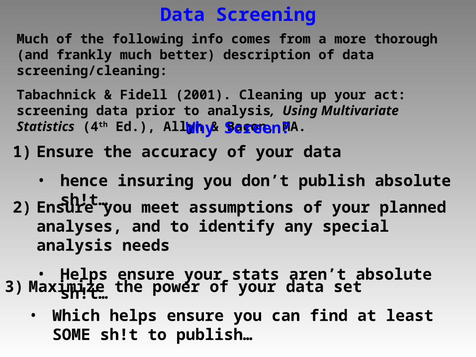
Data ScreeningMuch of the following info comes from a more thorough (and frankly much better) description of data screening/cleaning:

Tabachnick & Fidell (2001). Cleaning up your act: screening data prior to analysis, Using Multivariate Statistics (4th Ed.), Allyn & Bacon, MA.

Why Screen?

1) Ensure the accuracy of your data

• hence insuring you don’t publish absolute sh!t…

3) Maximize the power of your data set

• Which helps ensure you can find at least SOME sh!t to publish…

2) Ensure you meet assumptions of your planned analyses, and to identify any special analysis needs

• Helps ensure your stats aren’t absolute sh!t…

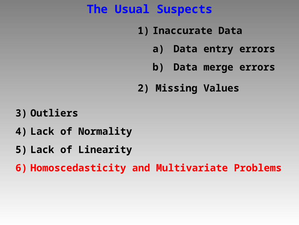
The Usual Suspects

1) Inaccurate Data

a) Data entry errors

b) Data merge errors

2) Missing Values

3) Outliers

4) Lack of Normality

5) Lack of Linearity

6) Homoscedasticity and Multivariate Problems

Avoiding Inaccurate Data1) KNOW WHAT YOUR DATA ARE SUPPOSED TO LOOK

LIKE

What possible values are (including range).

How many categories of subjects (controls, patients, etc) there should be.

How many subjects should be in each group.

2) Find out what your data DO look like..

Run Descriptives and Frequencies in SPSS

Can use “Explore” and/or “Crosstabs” option to look at values by Group

Example: Avoiding Inaccurate Data

1) Choose “Descriptive Statistics”

2) Choose “Explore”

3) Explore by “Factor List”

4) Enter variables you care about in “Dependent List”

5) Click on Display “Statistics”, “Plots”, or “Both”

6) And then on the appropriated tabs…

Yes, I realize the crossed arrows make for a terrible slide…

Example: Avoiding Inaccurate Data

7) Choose whatever you want, then click “continue”

8) It might be helpful to then click on options and choose “Report Missing Values”, then “continue” and “Ok”

What’s wrong with this picture?

Warnings

c1Fzf1t1 is constant when FH = 4. It will be included in any boxplots produced butother output will be omitted.

Look for any warnings

Case Processing Summary

48 96.0% 2 4.0% 50 100.0%

33 97.1% 1 2.9% 34 100.0%

36 100.0% 0 .0% 36 100.0%

2 100.0% 0 .0% 2 100.0%

FH1

2

3

4

c1Fzf1t1N Percent N Percent N Percent

Valid Missing Total

Cases

Any unexpected groups

Unexpected N’s Missing Values

What’s wrong with this picture?

These are ITC Data

Look for means and Standard Deviations that are very different from other groups.

Do these differences make any sense?

What’s wrong with this picture?Extreme Valuesa

4 .998

26 .347

2 .277

15 .275

1 .265

56 .061

21 .066

32 .069

16 .074

52 .075

76 .276

57 .266

20 .244

9 .235

84 .222

62 .056

55 .069

23 .074

78 .077

17 .089

119 .261

96 .245

89 .233

118 .231

91 .229

93 .063

103 .067

110 .069

114 .082

101 .088

121 1.620

122 1.450

1

2

3

4

5

1

2

3

4

5

1

2

3

4

5

1

2

3

4

5

1

2

3

4

5

1

2

3

4

5

1

1

Highest

Lowest

Highest

Lowest

Highest

Lowest

Highest

Lowest

FH1

2

3

4

c1Fzf1t1Case Number Value

The requested number of extreme values exceeds thenumber of data points. A smaller number of extremes isdisplayed.

a.

Look for extreme cases

Do they look like OUTLIERS or INNACURATE DATA?

Dealing With Missing Data Are missing values RANDOM or Systematic

E.G., are 2 subjects missing electrode F4, or are %50 of your ketamine group missing day two data…

Options if missing values are RANDOM:

1) Omit the case (but don’t DELETE it)

2) Substitute in a score

Of that subject’s scores (e.g., mean of other frontal electrodes)

Group mean (e.g., F4 mean of all other controls)

Substitute predicted score from regression

Lots of other more complicated substitution algorithms.

Dealing With Missing Data

Options if missing values are NOT RANDOM:

1) You’re pretty much screwed…regardless of your response to problem, it will effect the validity of the study.

However:

You might randomly delete subjects in other groups to match the sample sizes with your attenuated group.

Analyze data: both with and without missing cases

Treat missing data as a variable: Use of dummy variables in multiple regression models.

Outliers and Normality

Parametric Statistics (e.g., r, t-tests, ANOVA, Regressions) are built on the assumption of NORMALITY and LINEARITY…

If data are skewed or kurtotic, then this assumption is violated

If violation is large enough, it effects the accuracy of our results (typically towards making Type I errors).

Outliers (extreme scores) can be a major contributor to both (but particularly skewness)

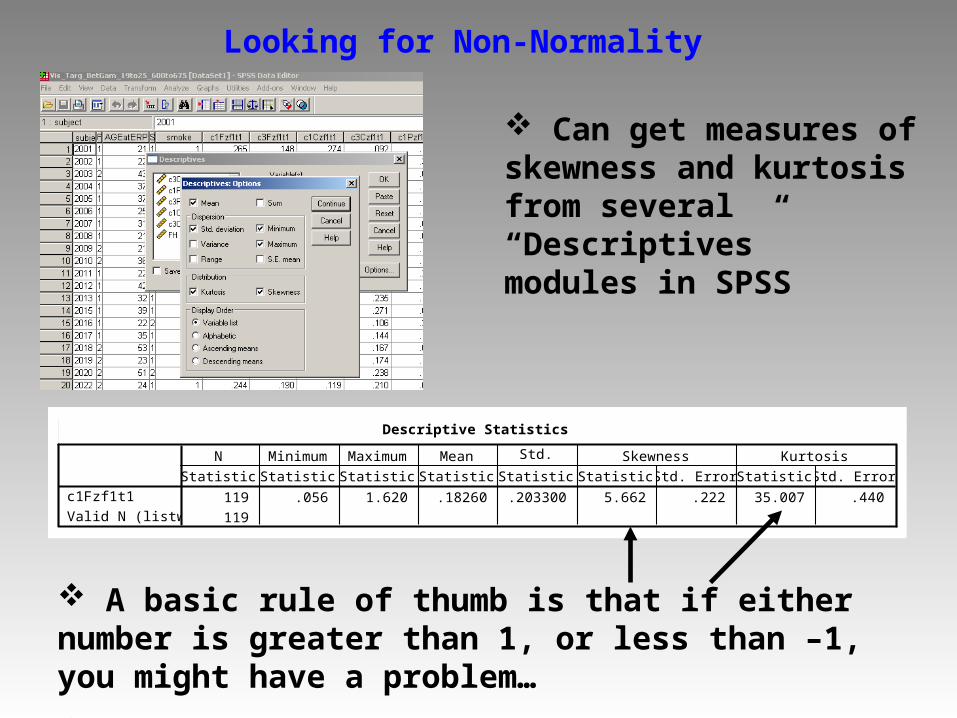
Looking for Non-Normality

Can get measures of skewness and kurtosis from several “Descriptives” modules in SPSS

Descriptive Statistics

119 .056 1.620 .18260 .203300 5.662 .222 35.007 .440

119

c1Fzf1t1

Valid N (listwise)

Statistic Statistic Statistic Statistic Statistic Statistic Std. Error Statistic Std. Error

N Minimum Maximum Mean Std.Deviation

Skewness Kurtosis

A basic rule of thumb is that if either number is greater than 1, or less than –1, you might have a problem…

However, dependent on sample size

Looking for Outliers Outliers can be detected using several SPSS routines, but

the easiest is by plotting your data (same for shape of distribution).

Two ways I like to do it

1) The Histogram

A. Go to “graphs” and then select “Histogram”

Looking for Outliers

B. Enter Variable you want to look at

C. I like to display the normal curve…

D. Then click “ok”

Any score falling outside the curve is an outlier


Another option is to “panel” by your Grouping variable…


2) The sneaky scatterplot method

Make sure your subject # variable is numeric

Plot subject number on X axis, and score of interest on Y

Easiest to do if you “Select Cases” in the data menu (e.g., look at each group one at a time)…

A. Go to “graphs” and then select “Scatter/Dot”

B. Choose the kind of plot you want and click “define”


C. Enter the variales you want and click “ok”


You’ll get a graph where you can easily see if there’s outliers….

D. By messing with the scale and chart size under the “chart editor” function (double click the graph on your output page), you can figure out the subject number of the outlier

Dealing with Outliers

1) Make sure it’s not a mistake (data entry error, impossible value, subject included in wrong group, etc.)

2) If it’s “real” data then you can:

Run with the data as is (and be sure you’re prepared to defend this choice)

Delete the case: this is dangerous ground, but can sometimes be justified (e.g., if z > 3…and again, be sure you can defend your choice)

Transform the data

Transformations Mathematical routine applied to ALL data in your set, designed to reduce effects of extreme values and/or kurtosis (helps for both skewness and kurtosis): Doesn’t effect relationship between scores!

Common Transformations:

1) Taking Square Root: Good for positive skew

2) Taking the Log10: Good for substantial positive skew

3) Taking the Inverse: good for severe positive skewness

Might need to add or subtract a constant from each score prior to transforming:

Add: if you have positively skewed data with some scores = 0

Subtract: If you’re dealing with negative skewness

Transformations

These transforms are done using “Compute” commands in SPSS…

Tabachnick and Fidel, Table 4.3

Example of a SPSS Transformation

1) Click on “transform”, and then “compute”

2) Name your new variable

3) Type in your expression

4) Click OK

Example of a SPSS Transformation

5) Rerun your descriptives, graphs, etc.


50 .061 .998 .17178 .139228 4.469 .337 25.629 .662

50

c1Fzf1t1

Valid N (listwise)



Skewness Kurtosis

Before:


50 .25 1.00 .3960 .12372 2.494 .337 10.489 .662

50

Fz_T1_SquareRoot

Valid N (listwise)



Skewness Kurtosis

After Square Root Transform:

If first you don’t succeed…


50 -1.21 .00 -.8374 .23054 .928 .337 2.070 .662

50

Fz_T1_Log

Valid N (listwise)



Skewness Kurtosis

After Log Transform

Linearity

The second major assumption of parametric stats is that relationships are LINEAR

If your data fail to meet this assumption the stats won’t work…even if there is a real relationship there…

Another reason why you want to plot out your data…

We’ll deal with multivariate linearity at some later lunch…

If all else fails: No matter how you transform them, your data are non-normal, or you see a non-linear relationship between your variables…

1) Run the data using parametric stats, but recognize (and describe/defend) limitations:

Use very conservative alpha levels (e.g., p <.001)

Treat your inferential stats primarily as descriptors…

2) Use nonparametric statistics

Stats Lunch: Day 2 Screening Your Data: Why and How.

Documents

Transcript of Stats Lunch: Day 2 Screening Your Data: Why and How.