Agenda

Nesterov’s method for the minimization of nonsmooth functions

1 Smoothing2 Conjugate functions3 Properties of conjugate functions4 Smoothing by conjugation5 Nesterov 2005 algorithm6 Examples

Nonsmooth optimization

minimize f(x)subject to x 2 C (can be Rn

)

f cvx, dom(f) = Rn

f not di↵erentiable

Examples

minimize kxk1subject to Ax = b

minimize kxkTV

subject to kx� bk2 �

minimize kAx� bk1

Objectives are not smooth

Motivation

f cvx with Lipschitz gradient,

O(

pL/✏)

iterations for ✏ approximation

f cvx and Lipshitz with cst. G,

O(G2/✏2)

iterations via method of subgradients for ✏ approximation

This lecture: speed up convergence for nonsmooth functions

Build smooth approximation fµ to objective functional

Minimize smooth approximation

Example: smoothed `

1

norm

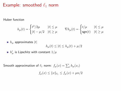
Huber function

hµ(t) =

(t2/2µ |t| µ

|t|� µ/2 |t| � µrhµ(t) =

(t/µ |t| µ

sgn(t) |t| � µ

hµ approximates |t|hµ(t) |t| hµ(t) + µ/2

h0µ is Lipschitz with constant 1/µ

Smooth approximation of `1 norm: fµ(x) =P

i hµ(xi)

fµ(x) kxk`1 fµ(x) + µn/2

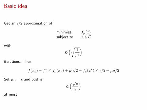
Basic idea

Get an ✏/2 approximation of

minimize fµ(x)subject to x 2 C

with

O⇣r

1

µ✏

⌘

iterations. Then

f(xk)� f? fµ(xk) + µn/2� fµ(x?) ✏/2 + µn/2

Set µn = ✏ and cost is

O⇣pn

✏

⌘

at most

References

Y. Nesterov. Smooth minimization of non-smooth functions, Math.

Program., Serie A, 103 (2005)

L. Vandenberghe. Lecture Notes for EE 236C, UCLA

S. Becker, E. Candes, and M. Grant. Templates for convex cone problemswith applications to sparse signal recovery. Mathematical Programming

Computation 3.3 (2011): 165–218.

Strongly convex functions

f is strongly cvx with parameter µ if for all x, y and all � 2 [0, 1]

f((1� �)x+ �y) (1� �)f(x) + �f(y)� µ�(1� �)

2

kx� yk2

For di↵erentiable functions, equivalent to

f(x) � f(y) + hrf(y), x� yi+ µ

2

kx� yk2 8x, y

For C2 functions, equivalent to

r2f(x) ⌫ µI 8x

A strongly cvx function has a unique minimizer

Conjugate of strongly convex functions

DefinitionConjugate of cvx f

f⇤(x) = sup

u2dom(f)hu, xi � f(u)

Lemma (Properties of conjugate of strongly convex functions)

Assume dom(f) cvx and closed

f⇤is well defined and di↵erentiable:

rf⇤(x) = u?

= arg max hu, xi � f(u)

rf⇤is Lipshitz and obeys

krf⇤(x)�rf⇤

(y)k2 µ�1kx� yk2

Proof. First,

f⇤(x+ h) = sup

u{hu, x+ hi � f(u)} � f⇤

(x) + hu?, hi

Second, we claim that because of strong convexity, h(u) = f(u)� hu, xi obeys

h(u) � h(u?) +

µ

2

ku� u?k2

(Easy to check if f is di↵erentiable.) Therefore,

f⇤(x+ h) = sup

u{hu, x+ hi � f(u)} f⇤

(x) + sup

u{hu, hi � µ

2

ku� u?k2}

= f⇤(x) + hu?, hi+ sup

v{hv, hi � µ

2

kvk2}

= f⇤(x) + hu?, hi+ 1

2µkhk22

Conclusion:

f⇤ is di↵erentiable and rf⇤(x) = u?

Lipschitz constant is at most 1/µ

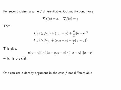
For second claim, assume f di↵erentiable. Optimality conditions

rf(u) = x, rf(v) = y

Then

f(v) � f(u) + hx, v � ui+ µ

2

ku� vk2

f(u) � f(v) + hy, u� vi+ µ

2

ku� vk2

This givesµku� vk2 hx� y, u� vi kx� yk ku� vk

which is the claim.

One can use a density argument in the case f not di↵erentiable

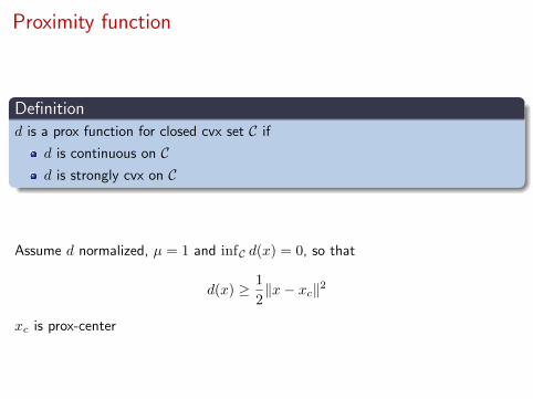
Proximity function

Definitiond is a prox function for closed cvx set C if

d is continuous on Cd is strongly cvx on C

Assume d normalized, µ = 1 and infC d(x) = 0, so that

d(x) � 1

2

kx� xck2

xc is prox-center

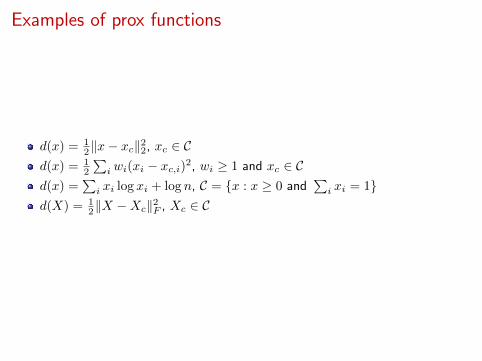
Examples of prox functions

d(x) = 12kx� xck22, xc 2 C

d(x) = 12

Pi wi(xi � xc,i)

2, wi � 1 and xc 2 Cd(x) =

Pi xi log xi + log n, C = {x : x � 0 and

Pi xi = 1}

d(X) =

12kX �Xck2F , Xc 2 C

Smoothing by conjugation

Suppose that f can be written as

f(x) = sup

u2dom(g)hu, xi � g(u) = g⇤(x)

Smooth approximation

fµ(x) = sup

u2dom(g)hu, xi � (g(u) + µd(u)) = (g + µd)⇤(x)

rfµ is Lipschitz with constant at most µ�1

if dom(g) bdd and D = supu2dom(g) d(u)

fµ(x) f(x) fµ(x) + µD

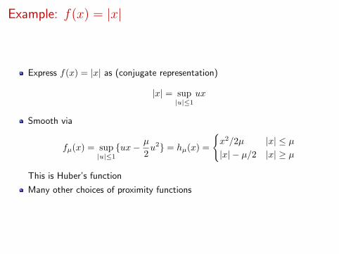
Example: f(x) = |x|

Express f(x) = |x| as (conjugate representation)

|x| = sup

|u|1ux

Smooth via

fµ(x) = sup

|u|1{ux� µ

2

u2} = hµ(x) =

(x2/2µ |x| µ

|x|� µ/2 |x| � µ

This is Huber’s function

Many other choices of proximity functions

Other representation

Express f(x) = |x| as (conjugate representation)

|x| = sup(u1 � u2)x u1, u2 � 0, u1 + u2 = 1

Proxd(u) = u1 log u1 + u2 log u2 + log 2

Smooth approximation

hµ(x) = µ log[cosh(x/µ)]

Smoothing norms

Pair of primal/dual norms f(x) = kxk = supkuk⇤1 hu, xi

fµ(x) = sup

kuk⇤1hu, xi � µd(u)

With `1 norm and d(u) = 12kuk22

fµ(x) = sup

kuk11hu, xi � µd(u) =

X

i

hµ(xi)

Suppose f(x) =P

i |xi � xi�1| = kDxk1, then

f(x) = sup

kuk11hD⇤u, xi

and smooth approximation

fµ(x) = sup

kuk11hD⇤u, xi � µd(u)

Complexity analysis

Want to find solution to nonsmooth problem with accuracy ✏

1 Construct smooth approximation such that

fµ(x) f(x) fµ(x) + µD

which givesf(x)� f? fµ(x)� f⇤

µ + µD

(rfµ is Lipschitz constant at most µ�1)2 Choose µ s.t. µD = ✏/2

3 Minimize fµ with accuracy ✏/2

Solution is ✏ accurate and number of iterations is

O⇣r

1

µ✏

⌘= O

⇣pD

✏

⌘

This is much better than O(1/✏2)

Example 1: Chebyshev approximation

minimize kAx� bk1A 2 Rm⇥n, b 2 Rm

Conjugate representation

f(x) = sup

(u,v)2Qhu� v,Ax� bi

Q = {(u, v) : u � 0, v � 0, 1Tu+ 1

T v = 1}Prox

d(u, v) =X

i

ui log ui +

X

i

vi log vi + log 2m

Smooth approximation: fµ(x) = sup(u,v)2Q{hu� v,Ax� bi � µd(u, v)}

fµ(x) = µ

mX

i=1

log

hcosh

⇣aTi x� biµ

⌘i

Accuracyfµ(x) f(x) fµ(x) + µ log 2m

E�cient Chebyshev approximation

Example 2: Robust regression

minimize kAx� bk1A 2 Rm⇥n, b 2 Rm

Conjugate representation

f(x) = sup

kuk11hu,Ax� bi

Prox

d(u) =1

2

kuk22Smooth approximation

fµ(x) = sup

kuk11{hu,Ax� bi � µkuk22} =

mX

i=1

hµ(aTi x� bi)

hµ is the Huber penalty function

Example 3: nuclear-norm minimization

minimize kXk⇤subject to A(X) = b

Conjugate representation

kXk⇤ =

X

i

�i(X) = sup

kUk1hU,Xi

Prox

d(U) =

1

2

kUk2FSmooth approximation

fµ(x) = sup

kUk1{hU,Xi � µ

2

kUk2F } =

mX

i=1

hµ(�i(X))

hµ is the Huber penalty function

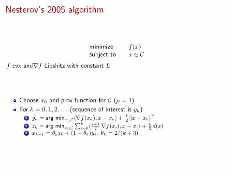
Nesterov’s 2005 algorithm

minimize f(x)subject to x 2 C

f cvx andrf Lipshitz with constant L

Choose x0 and prox function for C (µ = 1)

For k = 0, 1, 2, . . . (sequence of interest is yk)1

y

k

= arg minx2Chrf(x

k

), x� x

k

i+ L

2 kx� x

k

k22

z

k

= arg minx2C

Pk

i=0hi+12 rf(x

i

), x� x

i

i+ L

2 d(x)3

x

k+1 = ✓

k

z

k

+ (1� ✓

k

)yk

, ✓k

= 2/(k + 3)

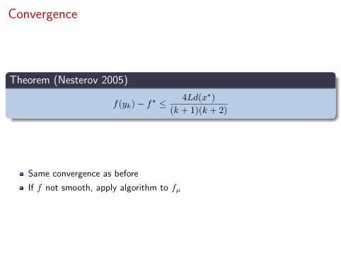
Convergence

Theorem (Nesterov 2005)

f(yk)� f? 4Ld(x⇤)

(k + 1)(k + 2)

Same convergence as before

If f not smooth, apply algorithm to fµ

Case study: total-variation denoising

Modelb = I + z

I is an n⇥ n image

z noise

b is the observed noisy image

Recovery via TV minimization (� is a bound on the noise level)

minimize kxkTV

subject to kx� bk2 �

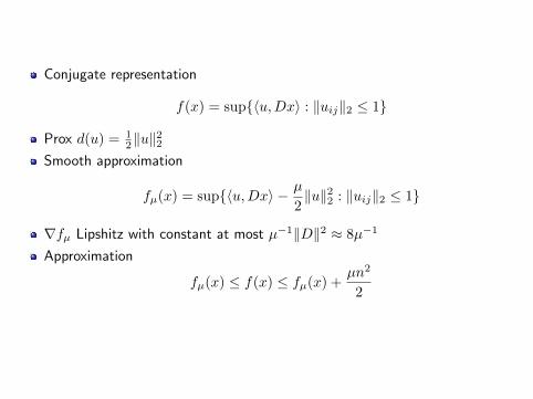
Conjugate representation

f(x) = sup{hu,Dxi : kuijk2 1}

Prox d(u) = 12kuk22

Smooth approximation

fµ(x) = sup{hu,Dxi � µ

2

kuk22 : kuijk2 1}

rfµ Lipshitz with constant at most µ�1kDk2 ⇡ 8µ�1

Approximation

fµ(x) f(x) fµ(x) +µn2

2

Nesterov’s method

minimize kxkTV

subject to kx� bk2 �

Choose x0 and for k = 0, 1, 2, . . . (sequence of interest is yk)1 Compute rfµ(xk) = DTuk

uk = arg max {uTDx� µ

2

kuk22 : kuijk2 1}

2 yk = arg min{hrfµ(xk), x� xki+ Lµ

2 kx� xkk2 : kx� bk2 �}3 zk = arg min {Pk

i=0h i+12 rfµ(xi), x� xii+ Lµ

2 kx� bk2 : kx� bk2 �}4 update xk+1 = ✓kzk + (1� ✓k)yk, ✓k = 2/(k + 3)

After change of variables, each step is of the form

minimize 12kxk22 � cTx subject to kxk2 t

with solution given bymin(1, t/kck2) c

Possible stopping criterion

Stop when PD gap less than a tol.

Dual problemminimize ��kDTuk2 + hb,DTuisubject to kuijk2 1

Duality gapkxk

TV

+ �kDTuk2 � hb,DTui