Analysis of Foreign Exchange Rates

with Functional Data Analysis

Statistics and Business project

Marina Doria G. Cortazar

Supervised by Pedro Galeano

June 2014

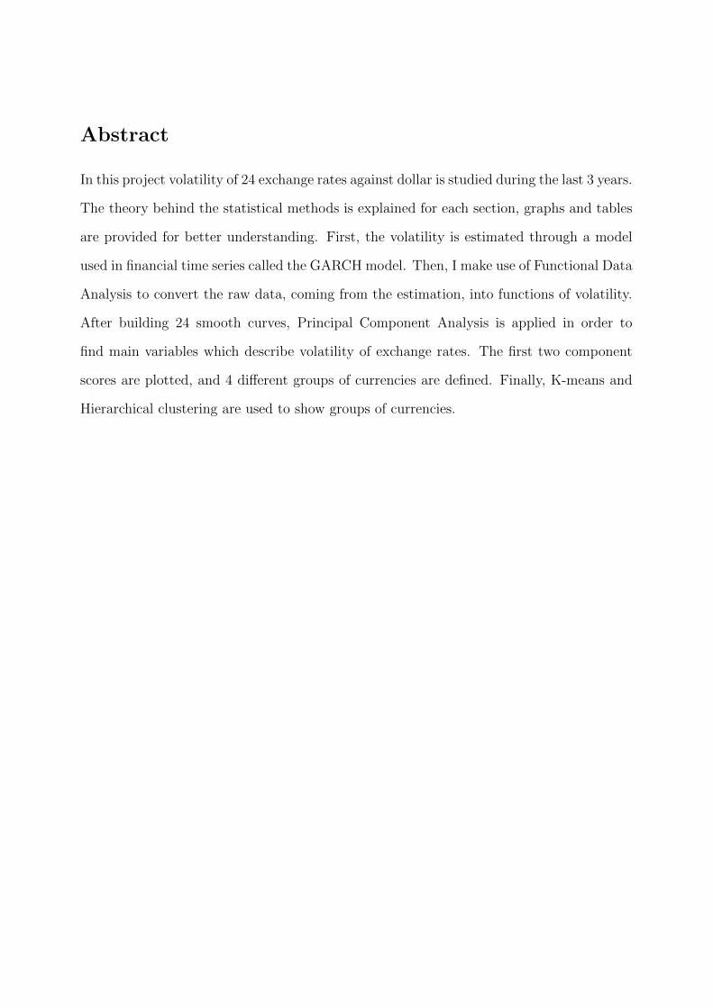
Abstract

In this project volatility of 24 exchange rates against dollar is studied during the last 3 years.

The theory behind the statistical methods is explained for each section, graphs and tables

are provided for better understanding. First, the volatility is estimated through a model

used in financial time series called the GARCH model. Then, I make use of Functional Data

Analysis to convert the raw data, coming from the estimation, into functions of volatility.

After building 24 smooth curves, Principal Component Analysis is applied in order to

find main variables which describe volatility of exchange rates. The first two component

scores are plotted, and 4 different groups of currencies are defined. Finally, K-means and

Hierarchical clustering are used to show groups of currencies.

Contents

1 Introduction 1

2 Data 3

3 Volatility estimation 6

4 Functional Data Analysis 9

4.1 What is Functional Data Analysis? . . . . . . . . . . . . . . . . . . . . . . 9

4.2 Functional volatility . . . . . . . . . . . . . . . . . . . . . . . . . . . . . . 10

4.3 Basis functions . . . . . . . . . . . . . . . . . . . . . . . . . . . . . . . . . 11

4.4 Fitting the data . . . . . . . . . . . . . . . . . . . . . . . . . . . . . . . . . 13

5 Functional Principal Component and Cluster Analyses 15

6 Conclusions 21

List of Figures

1 Euro ER against dollar. . . . . . . . . . . . . . . . . . . . . . . . . . . . . 5

2 Logarithm of 24 exchange rates. . . . . . . . . . . . . . . . . . . . . . . . . 5

3 Chilean and Brazilian ER logarithms. . . . . . . . . . . . . . . . . . . . . . 6

4 Estimated volatility σ of Euro ER. . . . . . . . . . . . . . . . . . . . . . . 8

5 Estimation of GARCH volatilities. . . . . . . . . . . . . . . . . . . . . . . . 8

6 Basic functions . . . . . . . . . . . . . . . . . . . . . . . . . . . . . . . . . 13

7 Euro ER functional volatility . . . . . . . . . . . . . . . . . . . . . . . . . 14

8 Exchange rate volatilities represented through 24 smooth curves. . . . . . . 15

9 First 4 Principal Component functions. . . . . . . . . . . . . . . . . . . . . 17

10 Principal Component scores. . . . . . . . . . . . . . . . . . . . . . . . . . . 18

11 K-means clustering. . . . . . . . . . . . . . . . . . . . . . . . . . . . . . . . 19

12 Cluster of exchange-rate volatilities during 3 years. . . . . . . . . . . . . . 20

13 Four groups of functional volatilities. . . . . . . . . . . . . . . . . . . . . . 21

List of Tables

1 Classification of currencies by their exchange rate regime. . . . . . . . . . . 3

2 Exchange rates against dollar. . . . . . . . . . . . . . . . . . . . . . . . . . 4

1 Introduction

This project aims to discover different groups of currencies depending on their exchange

rate volatility. The exchange rate is used to convert one currency into another. Moreover,

it is also regarded as the value of one country’s currency in terms of another country’s

currency. There are a wide variety of factors which influence the exchange rate, such as

interest rates, inflation, and the state of politics and the economy in each country, among

others. When one currency has a lower value than others, it means that products in this

country are cheaper for foreigners with stronger currency. This will cause the increasing

in exports and the country will gain competitiveness against others with higher currency

value. Currencies are another kind of financial assets, people can buy and sell them at

market’s prices (exchange-rates). High volatility in any financial asset is related with high

risk and low volatility with stability and free risk. Usually, buyers are confident about a

currency because the politic and economic environment of the country using this currency

is reliable. By contrast, countries with weak politic institutions may have high volatile

currencies as the risk of buying this currency is high (debt ratios change fast and prices for

foreign investors are unstable). Rogoff and Reinhart in This time is different (2010) claim

that high volatility in the exchange rate can cause a financial crisis in a country. Also,

further research have been done and some economists think that changes in exchange rates

can measure politic risk, see, for instance, Bloomberg and Hess (1997).

Before starting, it is important to know that there are two main groups (to put it

simple)1 of exchange rate regimes deliberated by Central Banks: Fixed and Float. A fixed

exchange rate means that the Central Bank of one currency decide to follow the value of

another because it is suitable for the country’s economy and therefore the exchange rate is

controlled. A float exchange rate is the one who is free of intervention. However, evidence

1I simplify the classification done by the International Monetary Fund. Mainly, I define Float ER to”Free Floating” and ”Floating” regimes. In the group of Fixed ER I include the rest of regimes. (Seereference [9])

1

suggest that most of the flexible exchange rates are highly “managed float”. For instance,

although euro/dollar is a free exchange rate, the European Central Bank and the Federal

Reserve try to maintain the currency constant to avoid speculate attacks. Through this

project I want to analyze the volatility of 24 floating and fixed exchange rates to discover

how these two groups differ in terms of volatility. Is it true that Fixed and Float exchange

rates are completely different in terms of volatility? Which are the most similar currencies?

Are there any outlier with very low or very high volatility?

For answering these questions I will make use of the tools provided by conditional

heteroscedastic volatility models and the functional data analysis (FDA). In particular,

we use Generalized AutoRegressive Conditional Heteroskedasticity (GARCH) type models,

proposed by Bollerslev (1986), to obtain estimates of the volatility of the 24 exchange rates,

that are then fitted using a basis of b-splines. Once this is done, I obtain functional principal

components of the functional volatilities that are used to obtain clusters of exchange rate

regimes.

The rest of this project is as follows. In Section 2, I present the dataset of exchange rates.

In Section 3, I make use of GARCH models to estimate the volatilities of each exchange

rate. In Section 4, I use b-splines to fit the estimates volatilities obtained in Section 3. In

Section 5, I obtain the functional principal components of the fitted estimated volatilities

and I use them to obtain clusters of exchange rates. Finally, Section 6 concludes.

2

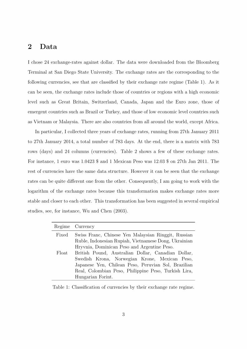
2 Data

I chose 24 exchange-rates against dollar. The data were downloaded from the Bloomberg

Terminal at San Diego State University. The exchange rates are the corresponding to the

following currencies, see that are classified by their exchange rate regime (Table 1). As it

can be seen, the exchange rates include those of countries or regions with a high economic

level such as Great Britain, Switzerland, Canada, Japan and the Euro zone, those of

emergent countries such as Brazil or Turkey, and those of low economic level countries such

as Vietnam or Malaysia. There are also countries from all around the world, except Africa.

In particular, I collected three years of exchange rates, running from 27th January 2011

to 27th January 2014, a total number of 783 days. At the end, there is a matrix with 783

rows (days) and 24 columns (currencies). Table 2 shows a few of these exchange rates.

For instance, 1 euro was 1.0423 $ and 1 Mexican Peso was 12.03 $ on 27th Jan 2011. The

rest of currencies have the same data structure. However it can be seen that the exchange

rates can be quite different one from the other. Consequently, I am going to work with the

logarithm of the exchange rates because this transformation makes exchange rates more

stable and closer to each other. This transformation has been suggested in several empirical

studies, see, for instance, Wu and Chen (2003).

Regime Currency

Fixed Swiss Franc, Chinese Yen Malaysian Ringgit, RussianRuble, Indonesian Rupiah, Vietnamese Dong, UkrainianHryvnia, Dominican Peso and Argentine Peso.

Float British Pound, Australian Dollar, Canadian Dollar,Swedish Krona, Norwegian Krone, Mexican Peso,Japanese Yen, Chilean Peso, Peruvian Sol, BrazilianReal, Colombian Peso, Philippine Peso, Turkish Lira,Hungarian Forint.

Table 1: Classification of currencies by their exchange rate regime.

3

Date Euro Mexican Peso Japanese Yen Chilean Peso27 Jan 11 1.3734 12.0371 82.92 485.328 Jan 11 1.3611 12.2062 82.12 484.3529 Jan 11 1.3694 12.1219 82.04 483.27··· ··· ··· ··· ···

25 Jan 14 1.3696 13.4018 103.26 549.1926 Jan 14 1.3678 13.46 102.31 550.627 Jan 14 1.3673 13.366 102.55 549.71

Table 2: Exchange rates against dollar.

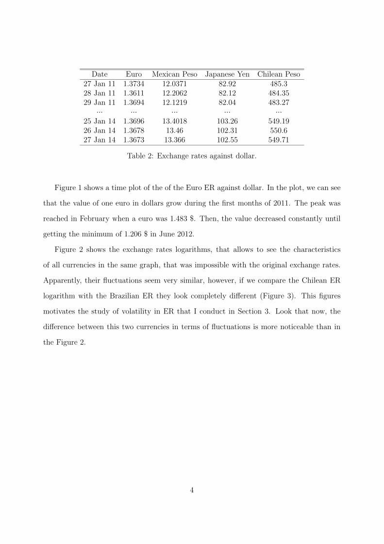
Figure 1 shows a time plot of the of the Euro ER against dollar. In the plot, we can see

that the value of one euro in dollars grow during the first months of 2011. The peak was

reached in February when a euro was 1.483 $. Then, the value decreased constantly until

getting the minimum of 1.206 $ in June 2012.

Figure 2 shows the exchange rates logarithms, that allows to see the characteristics

of all currencies in the same graph, that was impossible with the original exchange rates.

Apparently, their fluctuations seem very similar, however, if we compare the Chilean ER

logarithm with the Brazilian ER they look completely different (Figure 3). This figures

motivates the study of volatility in ER that I conduct in Section 3. Look that now, the

difference between this two currencies in terms of fluctuations is more noticeable than in

the Figure 2.

4

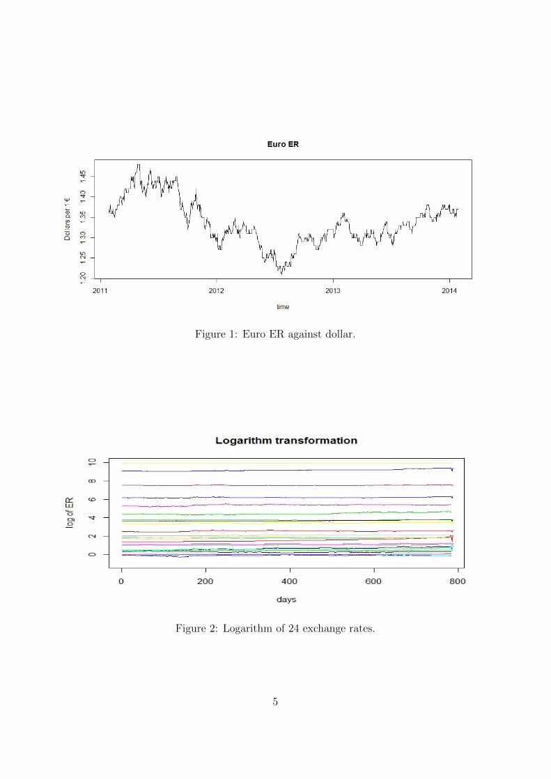
Figure 1: Euro ER against dollar.

Figure 2: Logarithm of 24 exchange rates.

5

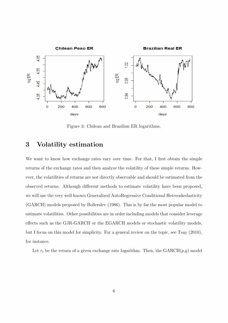
Figure 3: Chilean and Brazilian ER logarithms.

3 Volatility estimation

We want to know how exchange rates vary over time. For that, I first obtain the simple

returns of the exchange rates and then analyze the volatility of these simple returns. How-

ever, the volatilities of returns are not directly observable and should be estimated from the

observed returns. Although different methods to estimate volatility have been proposed,

we will use the very well known Generalized AutoRegressive Conditional Heteroskedasticity

(GARCH) models proposed by Bollerslev (1986). This is by far the most popular model to

estimate volatilities. Other possibilities are in order including models that consider leverage

effects such as the GJR-GARCH or the EGARCH models or stochastic volatility models,

but I focus on this model for simplicity. For a general review on the topic, see Tsay (2010),

for instance.

Let rt be the return of a given exchange rate logarithm. Then, the GARCH(p,q) model

6

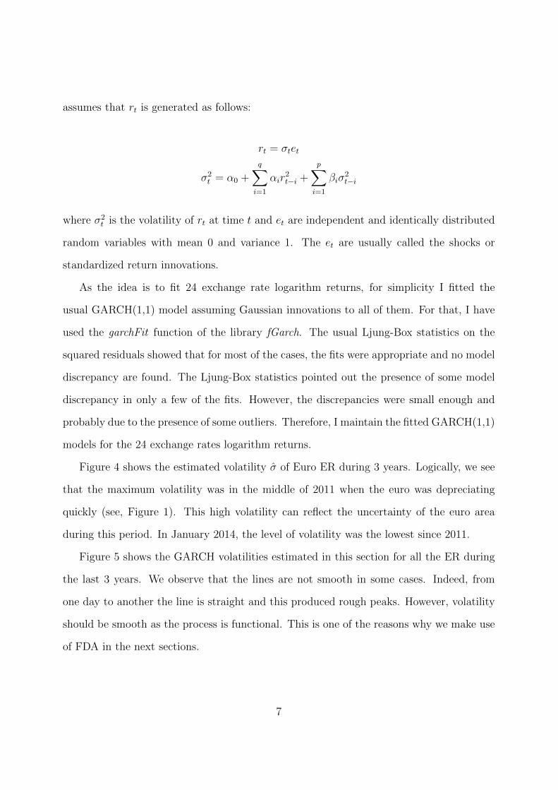
assumes that rt is generated as follows:

rt = σtet

σ2t = α0 +

q∑i=1

αir2t−i +

p∑i=1

βiσ2t−i

where σ2t is the volatility of rt at time t and et are independent and identically distributed

random variables with mean 0 and variance 1. The et are usually called the shocks or

standardized return innovations.

As the idea is to fit 24 exchange rate logarithm returns, for simplicity I fitted the

usual GARCH(1,1) model assuming Gaussian innovations to all of them. For that, I have

used the garchFit function of the library fGarch. The usual Ljung-Box statistics on the

squared residuals showed that for most of the cases, the fits were appropriate and no model

discrepancy are found. The Ljung-Box statistics pointed out the presence of some model

discrepancy in only a few of the fits. However, the discrepancies were small enough and

probably due to the presence of some outliers. Therefore, I maintain the fitted GARCH(1,1)

models for the 24 exchange rates logarithm returns.

Figure 4 shows the estimated volatility σ of Euro ER during 3 years. Logically, we see

that the maximum volatility was in the middle of 2011 when the euro was depreciating

quickly (see, Figure 1). This high volatility can reflect the uncertainty of the euro area

during this period. In January 2014, the level of volatility was the lowest since 2011.

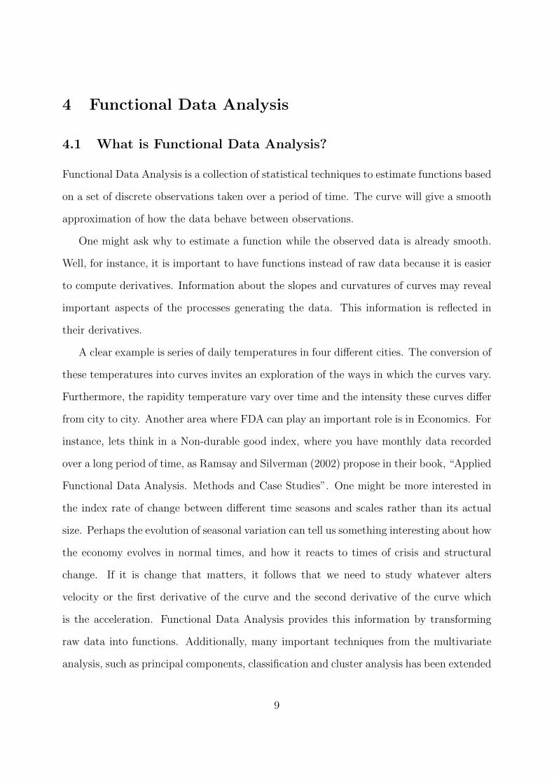
Figure 5 shows the GARCH volatilities estimated in this section for all the ER during

the last 3 years. We observe that the lines are not smooth in some cases. Indeed, from

one day to another the line is straight and this produced rough peaks. However, volatility

should be smooth as the process is functional. This is one of the reasons why we make use

of FDA in the next sections.

7

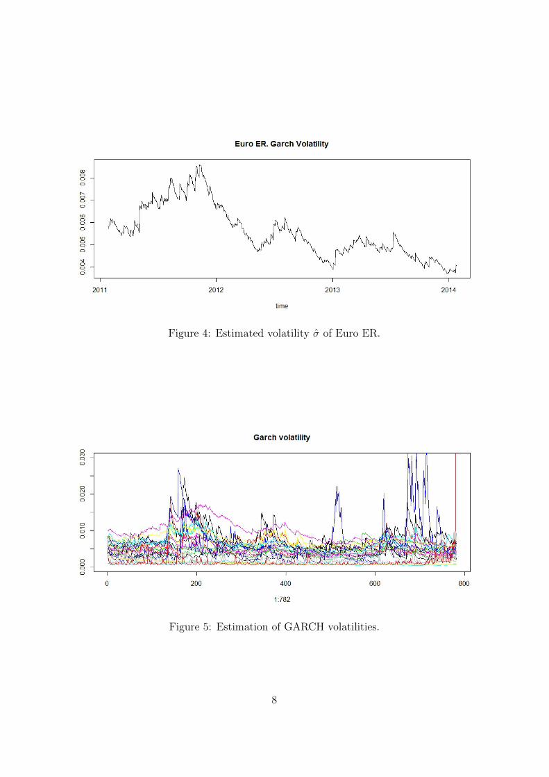
Figure 4: Estimated volatility σ of Euro ER.

Figure 5: Estimation of GARCH volatilities.

8

4 Functional Data Analysis

4.1 What is Functional Data Analysis?

Functional Data Analysis is a collection of statistical techniques to estimate functions based

on a set of discrete observations taken over a period of time. The curve will give a smooth

approximation of how the data behave between observations.

One might ask why to estimate a function while the observed data is already smooth.

Well, for instance, it is important to have functions instead of raw data because it is easier

to compute derivatives. Information about the slopes and curvatures of curves may reveal

important aspects of the processes generating the data. This information is reflected in

their derivatives.

A clear example is series of daily temperatures in four different cities. The conversion of

these temperatures into curves invites an exploration of the ways in which the curves vary.

Furthermore, the rapidity temperature vary over time and the intensity these curves differ

from city to city. Another area where FDA can play an important role is in Economics. For

instance, lets think in a Non-durable good index, where you have monthly data recorded

over a long period of time, as Ramsay and Silverman (2002) propose in their book, “Applied

Functional Data Analysis. Methods and Case Studies”. One might be more interested in

the index rate of change between different time seasons and scales rather than its actual

size. Perhaps the evolution of seasonal variation can tell us something interesting about how

the economy evolves in normal times, and how it reacts to times of crisis and structural

change. If it is change that matters, it follows that we need to study whatever alters

velocity or the first derivative of the curve and the second derivative of the curve which

is the acceleration. Functional Data Analysis provides this information by transforming

raw data into functions. Additionally, many important techniques from the multivariate

analysis, such as principal components, classification and cluster analysis has been extended

9

to the functional framework, see, for instance, Ramsay and Silverman (2002) and Ferraty

and Vieu (2006).

In our example, we will be working with volatility of foreign exchange rates. The Foreign

Exchange Market (FX) is unique because its huge volume trade represents the largest asset

class in the world. All these financial transactions are public and recorded, therefore we

end with multiple data in a period of time. This study focuses in analyzing the volatility

of exchange rates. We assume that volatility is functional because from one observation

to the next the process is smooth. The goal is to transform discrete volatility records into

functions of volatility to have a deeply understanding of how this curves change along 3

years.

The goals of functional data analysis are essentially the same as those of any other

branch of statistics: represent the data, study patterns and variations among the data and

find groups with similar characteristics. In particular we are interested in:

• Represent exchange rates in ways that aid further analysis.

• Display data in order to find characteristics of each currency.

• Study sources of pattern and variation among exchange rates.

• Find groups of currencies with similar performance.

• Argument our results with economic reasoning.

4.2 Functional volatility

Now, for each one of the exchange rate logarithm returns, I have 783 estimated volatilities2.

Therefore, for each return series, I have a series of estimated volatilities σ2(1), σ2(2), ..., σ2(783).

2A total of 784 exchange rate daily values are reduced to 783 volatility values because we need tomeasure differences between days.

10

As mentioned before, the estimated volatilities are somehow rough. Therefore, my next

goal is to smooth the estimated volatilities, as basically, the volatilities can be seen as a

continuous smooth process in which jumps are rare. Therefore, for each return series, I am

looking for a function x(t) such that:

σ2(tj) = x(tj) + ε(tj)

where tj = 1, . . . , 783 and ε(t) is a noise function evaluated at the observed points. In

particular, I assume that the ε’s are independent and identically distributed with zero

mean and constant variance. Consequently, we want to obtain 24 sets of 783 pairs of the

form (tj, xi(tj)), where i = 1, . . . , 24 and j = 1, . . . , 783, where the xi are smooth functions

that approximate the estimated volatilities from exchange rate logarithm return i.

For that, I make use of the tools of the Functional Data Analysis (FDA). Note that I

consider this approach because posteriorly I want to perform cluster analysis on the smooth

functions to make groups of similar currencies in terms of volatilities. This goal can be

accomplished using the tools of the FDA as I will present in Sections 5.

The next section will explain the process of transforming the 24 discrete exchange rate

volatilities into smooth functions using the following two steps:

1. Representing functions by basic functions.

2. Fitting a curve to the data through a vector, matrix, or array of coefficients which

defines the function as a linear combination of these functions.

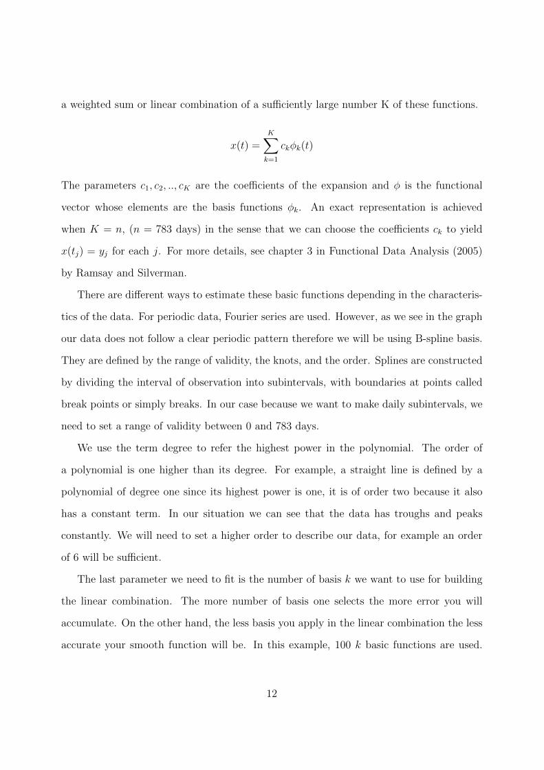
4.3 Basis functions

A basis function system is a set of known functions φk that are mathematically independent

of each other and that have the property that we can approximate any function by taking

11

a weighted sum or linear combination of a sufficiently large number K of these functions.

x(t) =K∑k=1

ckφk(t)

The parameters c1, c2, .., cK are the coefficients of the expansion and φ is the functional

vector whose elements are the basis functions φk. An exact representation is achieved

when K = n, (n = 783 days) in the sense that we can choose the coefficients ck to yield

x(tj) = yj for each j. For more details, see chapter 3 in Functional Data Analysis (2005)

by Ramsay and Silverman.

There are different ways to estimate these basic functions depending in the characteris-

tics of the data. For periodic data, Fourier series are used. However, as we see in the graph

our data does not follow a clear periodic pattern therefore we will be using B-spline basis.

They are defined by the range of validity, the knots, and the order. Splines are constructed

by dividing the interval of observation into subintervals, with boundaries at points called

break points or simply breaks. In our case because we want to make daily subintervals, we

need to set a range of validity between 0 and 783 days.

We use the term degree to refer the highest power in the polynomial. The order of

a polynomial is one higher than its degree. For example, a straight line is defined by a

polynomial of degree one since its highest power is one, it is of order two because it also

has a constant term. In our situation we can see that the data has troughs and peaks

constantly. We will need to set a higher order to describe our data, for example an order

of 6 will be sufficient.

The last parameter we need to fit is the number of basis k we want to use for building

the linear combination. The more number of basis one selects the more error you will

accumulate. On the other hand, the less basis you apply in the linear combination the less

accurate your smooth function will be. In this example, 100 k basic functions are used.

12

Through these 100 basic functions we will be able to plot smooth exchange rate volatilities.

Figure 6: 100 basic functions with an order of 6 during 783 days.

4.4 Fitting the data

Remember that our goal is to fit the discrete observations using the model σ2 = x(tj)+ε(tj).

We saw that for the term x(tj) we apply a basis function expansion x(t) =K∑k=1

ckφk(t).

However we still need to obtain the coefficients of ck to complete our linear combination.

The simplest method Ramsay and Silverman give in their book (Functional Data Analysis,

2005) is by minimizing the least square criterion:

SMSSE(σ2|c) =n∑

j=1

[σ2j −

K∑k=1

ckφk(tj)]2

In matrix form,

SMSSE(σ2|c) = (σ2 − Φc)′(σ2 − Φc) = ||σ2 − Φc||2

13

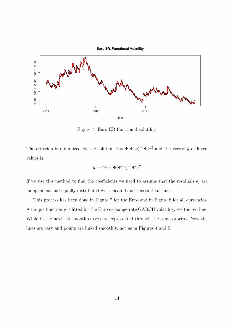
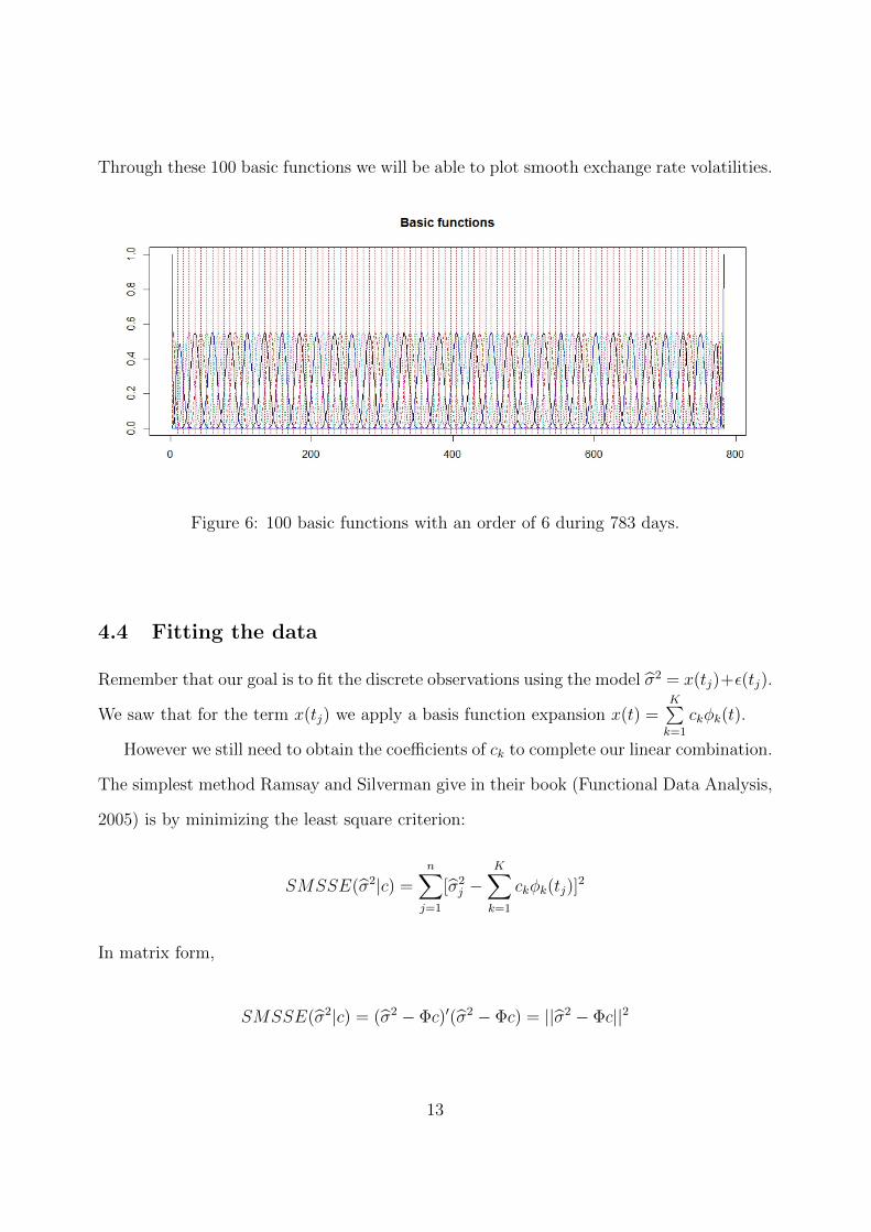
Figure 7: Euro ER functional volatility

The criterion is minimized by the solution c = Φ(Φ′Φ)−1Φ′σ2 and the vector y of fitted

values is:

y = Φˆc = Φ(Φ′Φ)−1Φ′σ2

If we use this method to find the coefficients we need to assume that the residuals εj are

independent and equally distributed with mean 0 and constant variance.

This process has been done in Figure 7 for the Euro and in Figure 8 for all currencies.

A unique function y is fitted for the Euro exchange-rate GARCH volatility, see the red line.

While in the next, 24 smooth curves are represented through the same process. Now the

lines are easy and points are linked smoothly, not as in Figures 4 and 5.

14

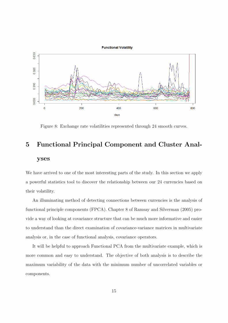
Figure 8: Exchange rate volatilities represented through 24 smooth curves.

5 Functional Principal Component and Cluster Anal-

yses

We have arrived to one of the most interesting parts of the study. In this section we apply

a powerful statistics tool to discover the relationship between our 24 currencies based on

their volatility.

An illuminating method of detecting connections between currencies is the analysis of

functional principle components (FPCA). Chapter 8 of Ramsay and Silverman (2005) pro-

vide a way of looking at covariance structure that can be much more informative and easier

to understand than the direct examination of covariance-variance matrices in multivariate

analysis or, in the case of functional analysis, covariance operators.

It will be helpful to approach Functional PCA from the multivariate example, which is

more common and easy to understand. The objective of both analysis is to describe the

maximum variability of the data with the minimum number of uncorrelated variables or

components.

15

Multivariate principal components are defined as

fi = β′xi =∑j=1

βjxij,

for i = 1, 2..., N where β is the vector (β1, ...., βp)′ and xi is the vector (xi1, ...., xip)

′ con-

taining the values of the variables.

In our case we are working with functional data, where β(s) and x(s) are functions and

summations over j are replaced by integrations over s to define the inner product:

fi =

∫βx =

∫β(s)x(s)ds

In particular, we are interested in maximizing the variance in the f ′is. The objective

is finding the weight vector ξ1 = (ξ11, ..., ξp1)′ located in the linear combinations fi1 =∫

ξ1(s)x(s)ds. At the same time we maximize the square of N−1∑

i f2i = N−1

∑i

∫(ξ1x1)

2

subject to the constraint∫

(ξ1(s))2 = 1.

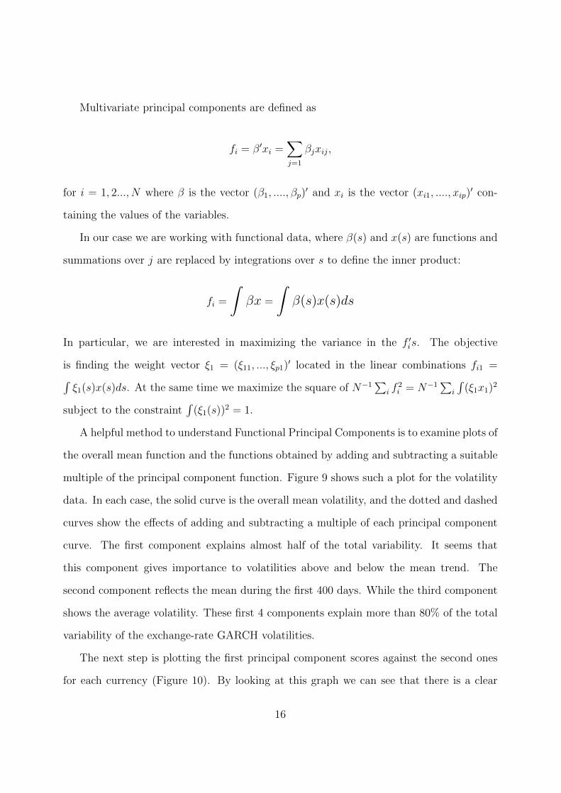
A helpful method to understand Functional Principal Components is to examine plots of

the overall mean function and the functions obtained by adding and subtracting a suitable

multiple of the principal component function. Figure 9 shows such a plot for the volatility

data. In each case, the solid curve is the overall mean volatility, and the dotted and dashed

curves show the effects of adding and subtracting a multiple of each principal component

curve. The first component explains almost half of the total variability. It seems that

this component gives importance to volatilities above and below the mean trend. The

second component reflects the mean during the first 400 days. While the third component

shows the average volatility. These first 4 components explain more than 80% of the total

variability of the exchange-rate GARCH volatilities.

The next step is plotting the first principal component scores against the second ones

for each currency (Figure 10). By looking at this graph we can see that there is a clear

16

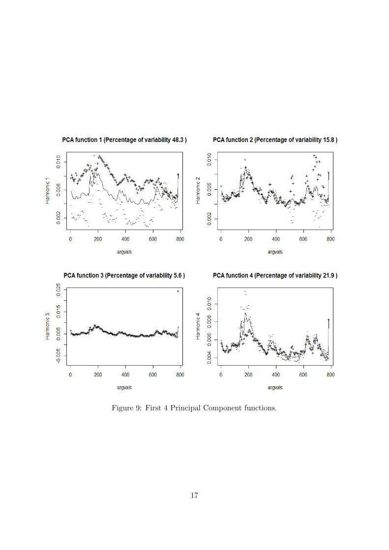
Figure 9: First 4 Principal Component functions.

17

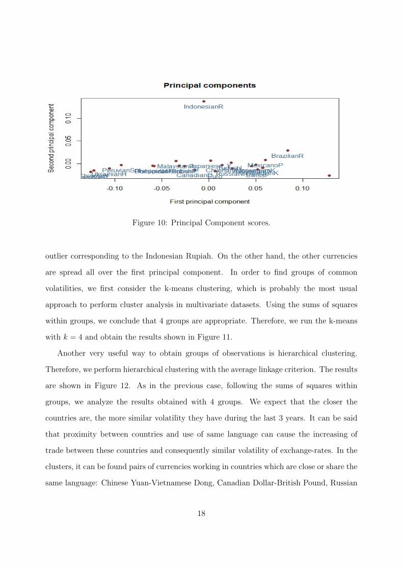
Figure 10: Principal Component scores.

outlier corresponding to the Indonesian Rupiah. On the other hand, the other currencies

are spread all over the first principal component. In order to find groups of common

volatilities, we first consider the k-means clustering, which is probably the most usual

approach to perform cluster analysis in multivariate datasets. Using the sums of squares

within groups, we conclude that 4 groups are appropriate. Therefore, we run the k-means

with k = 4 and obtain the results shown in Figure 11.

Another very useful way to obtain groups of observations is hierarchical clustering.

Therefore, we perform hierarchical clustering with the average linkage criterion. The results

are shown in Figure 12. As in the previous case, following the sums of squares within

groups, we analyze the results obtained with 4 groups. We expect that the closer the

countries are, the more similar volatility they have during the last 3 years. It can be said

that proximity between countries and use of same language can cause the increasing of

trade between these countries and consequently similar volatility of exchange-rates. In the

clusters, it can be found pairs of currencies working in countries which are close or share the

same language: Chinese Yuan-Vietnamese Dong, Canadian Dollar-British Pound, Russian

18

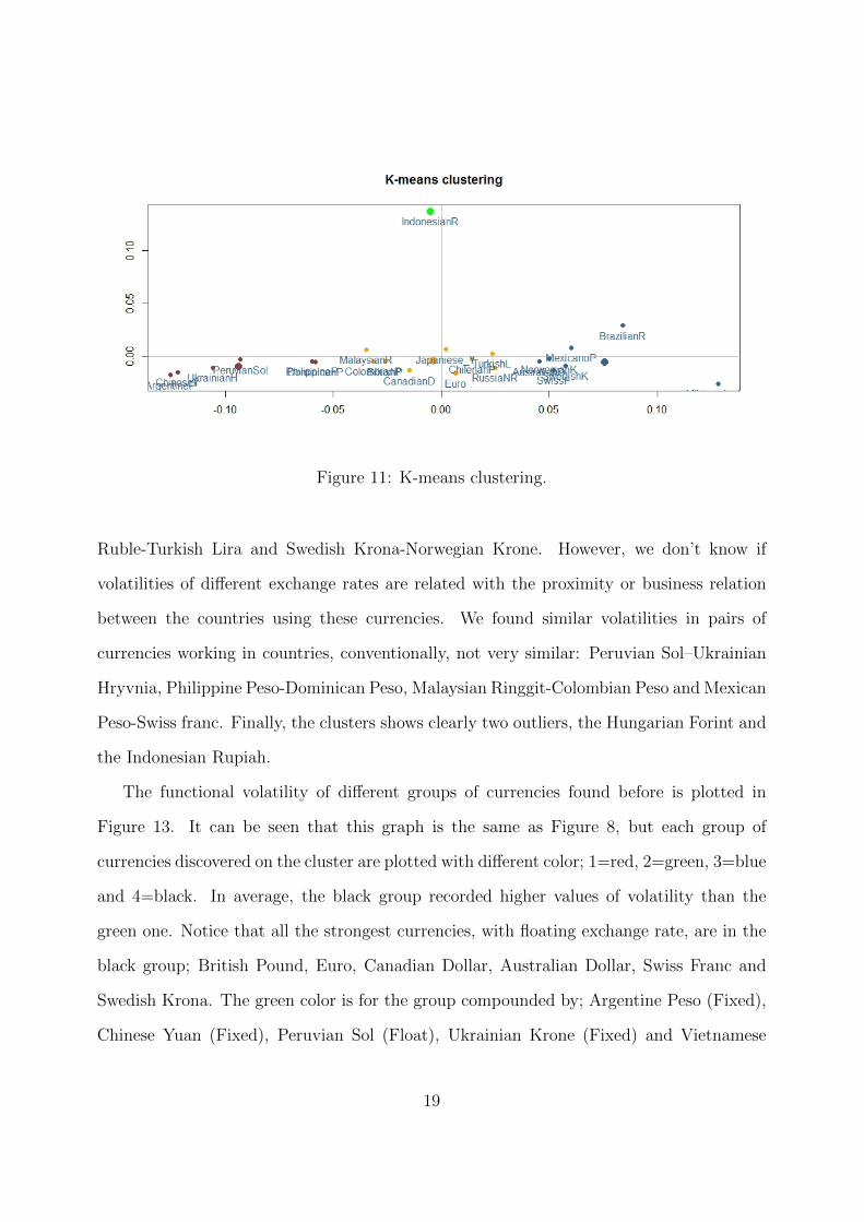
Figure 11: K-means clustering.

Ruble-Turkish Lira and Swedish Krona-Norwegian Krone. However, we don’t know if

volatilities of different exchange rates are related with the proximity or business relation

between the countries using these currencies. We found similar volatilities in pairs of

currencies working in countries, conventionally, not very similar: Peruvian Sol–Ukrainian

Hryvnia, Philippine Peso-Dominican Peso, Malaysian Ringgit-Colombian Peso and Mexican

Peso-Swiss franc. Finally, the clusters shows clearly two outliers, the Hungarian Forint and

the Indonesian Rupiah.

The functional volatility of different groups of currencies found before is plotted in

Figure 13. It can be seen that this graph is the same as Figure 8, but each group of

currencies discovered on the cluster are plotted with different color; 1=red, 2=green, 3=blue

and 4=black. In average, the black group recorded higher values of volatility than the

green one. Notice that all the strongest currencies, with floating exchange rate, are in the

black group; British Pound, Euro, Canadian Dollar, Australian Dollar, Swiss Franc and

Swedish Krona. The green color is for the group compounded by; Argentine Peso (Fixed),

Chinese Yuan (Fixed), Peruvian Sol (Float), Ukrainian Krone (Fixed) and Vietnamese

19

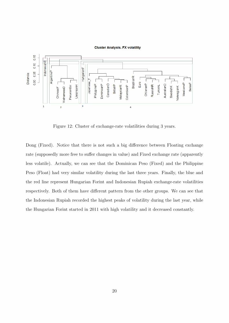
Figure 12: Cluster of exchange-rate volatilities during 3 years.

Dong (Fixed). Notice that there is not such a big difference between Floating exchange

rate (supposedly more free to suffer changes in value) and Fixed exchange rate (apparently

less volatile). Actually, we can see that the Dominican Peso (Fixed) and the Philippine

Peso (Float) had very similar volatility during the last three years. Finally, the blue and

the red line represent Hungarian Forint and Indonesian Rupiah exchange-rate volatilities

respectively. Both of them have different pattern from the other groups. We can see that

the Indonesian Rupiah recorded the highest peaks of volatility during the last year, while

the Hungarian Forint started in 2011 with high volatility and it decreased constantly.

20

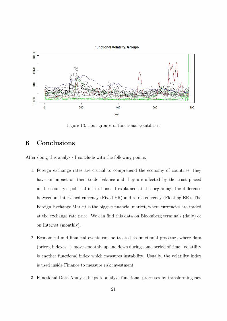
Figure 13: Four groups of functional volatilities.

6 Conclusions

After doing this analysis I conclude with the following points:

1. Foreign exchange rates are crucial to comprehend the economy of countries, they

have an impact on their trade balance and they are affected by the trust placed

in the country’s political institutions. I explained at the beginning, the difference

between an intervened currency (Fixed ER) and a free currency (Floating ER). The

Foreign Exchange Market is the biggest financial market, where currencies are traded

at the exchange rate price. We can find this data on Bloomberg terminals (daily) or

on Internet (monthly).

2. Economical and financial events can be treated as functional processes where data

(prices, indexes...) move smoothly up and down during some period of time. Volatility

is another functional index which measures instability. Usually, the volatility index

is used inside Finance to measure risk investment.

3. Functional Data Analysis helps to analyze functional processes by transforming raw

21

data into smooth functions. By working with functions, we are able to estimate

any value at any point in time. In particular, I showed how to built 24 volatility

functions taken from discrete exchange rate values during 3 years. First, computing

the GARCH volatility model (raw data), and then transforming 24× 784 values into

24 unique functions.

4. The most important section of the paper was discovering different groups of currencies

depending on their volatility along 3 years. Knowing that currencies are intervened

by central banks, I decided to study volatility of exchange rates because in practice,

there is not such a difference between Floating exchange rate (supposedly more free to

suffer changes in value) and Fixed exchange rate (apparently less volatile). Actually,

after doing the Functional Principal Component Analysis, I saw in the cluster that

the Dominican Peso (Fixed ER with the dollar) and the Philippine Peso (Floating

ER) had very similar volatility during the last three years. Also, it is important

to notice that through this analysis we can find outliers like the Indonesian Rupee

(Floating ER) and the Hungarian Forint (Floating ER).

5. Functional Data Analysis can be helpful to discover patterns in Finance and Eco-

nomics. Each day the financial market produces huge amount of data, sometimes full

of noise. It would be useful to find trends by working with smooth functions. As well

as, finding second derivatives to see acceleration in some indexes or prices. This is

an ambitious topic, because data in Finance and Economics is produced by people

actions and expectations, which I personally think are difficult to estimate.

References

[1] Reinhart, C. M. and Rogoff, K. S. (2010) This Time Is Different: Eight Centuries of

Financial Folly. Princeton University Press.

22

[2] Bloomberg, S. B. and Hess, G. (1997) Politics and Exchange Rate Forecasts. Journal

of International Economics, 43, 89-205.

[3] Bollerslev, T. (1986) Generalized Autoregressive Conditional Heteroskedasticity. Jour-

nal of Econometrics, 31, 307-327.

[4] Ramsay, J. O. and Silverman, B. W. (2002) Applied Functional Data Analysis. Methods

and Case Studies. Springer.

[5] Ramsay, J. O. and Silverman, B. W. (2005) Functional Data Analysis. Springer.

[6] Ramsay, J. O., Hooker, G. and Graves, S. (2009) Functional Data Analysis with R and

MATLAB. Springer.

[7] Tsay, R. S. (2010) Analysis of Financial Time Series. John Wiley and Sons.

[8] Wu, J.-L. and Chen, S.-L. (2003) Real Exchange-Rate Prediction over Short Horizons.

Review of International Economics, 9, 401-413.

[9] International Monetary Fund (2013) Annual Report on Exchange Arrangements and

Exchange Restrictions.

23