Statistics in Retail Finance Chapter 6: Behavioural...

Statistics in Retail Finance Chapter 6: Behavioural models

1

Statistics in Retail Finance

Chapter 6: Behavioural models


2

Overview >

So far we have focussed mainly on application scorecards.

In this chapter we shall look at behavioural models.

We shall cover the following topics:-

Behavioural models and data;

Static behavioural models;

Dynamic models of behaviour:

o Survival models;

o Markov transition models.


3

Why Behavioural Models? >

Application scorecards only deal with application processing, deciding

whether to accept or reject an application for credit.

However, once a borrower is given credit, their behaviour needs to be

monitored in terms of credit usage and repayments.

There are several reasons for this:

Risk assessment. It allows the lender to update their assessment of

risk and warn of possible problems in the future.

Operational decisions. The lender can choose to adjust lending

parameters such as credit limit or interest rate, based on borrower

behaviour.


4

Marketing and customer relations. Offer new products to existing

“good” customers, and respond to customer requests for new products

or changes in credit limit and interest rate.

Risk management. Estimation of default rate on loan portfolio and

calculation of capital requirements.


5

Behavioural Models of Default or Delinquincy >

Rather like application scorecards, behavioural models are usually models of

default, or possibly, delinquency.

Values of predictor variables are taken across a performance period of

the loan up to a pre-specified observation point.

The outcome variable (usually, default / non-default) is taken at an

outcome point some time after the observation point.

Calendar Time

Borrower behaviour

Observation

Point

Observation Period Outcome

Point

Outcome?


6

What does the dynamic behaviour of credit accounts look like?

Example 6.1

Here is a case study of a credit card account. Notice how erratic credit card

usage is.

Values are fictional but based on a true account.

0

1000

2000

3000

4000

5000

0 5 10 15 20 25 30 35 40

£

Months account open

Balance Credit limit Repayment Debits


7

Example 6.2

Here is another case study of a credit card account. Notice this time, card

usage has some structure, but eventually the credit card holder defaults at

32 months.

Values are fictional but based on a true account.

0

1

2

3

0

500

1000

1500

2000

0 5 10 15 20 25 30 35

Mo

nth

s

£

Months account open

Balance Credit limit Repayment Debits Missed payments (months)


8

Static Behavioural Models >

Traditionally, behavioural models have been built using the same kind of

static models as are used in application scoring.

For example, typically, logistic regression is used.

The outcome of such a model is a behavioural score.

Since values of predictor variables change over the performance period,

aggregate values are used:

o eg mean, maximum or last values of variables over time.


9

Typical Behavioural Variables >

Some typical aggregate variables used in static behavioural models are:-

The application variables;

Generic credit score;

Last current balance (ie at the end of the performance period);

Mean balance;

Last balance / starting balance ratio;

Sum of credit advances;

Mean monthly repayment amount;

Total number of missed payments;

Total number of months that credit limit is exceeded (for credit card).

The number of potential predictor variables can get quite large for

behavioural models, so automated variable selection may be required to

reduce their number.


10

Dynamic Models >

In many ways, using static models based on aggregates on variables that

naturally occur over time is missing a great opportunity, since these models

will not fully represent the dynamic quality of the data.

There are several statistical models that allow us to naturally model

behaviour over time.

Two modelling approaches which are finding favour in the industry are:

Survival model;

Markov transition model.

We will cover each of these models in this chapter.

Not only do dynamic models have the advantage that they can take account

of changes in credit use over time, they can be used as the basis of profit

estimation. This is covered in the next chapter.


11

Survival Models of time to default >

Interest in using survival analysis for credit scoring is quite recent.

Survival models allow us to model not just if a borrower will default,

but when.

The advantages of using survival models are that:-

1. They naturally model the loan default process and so incorporate situations when a case has not defaulted in the observation period;

2. Their use avoids the need to define a fixed period within which default

is measured;

3. They provide a clear approach to assess the expected profitability of a

borrower;


12

4. Survival estimates provide a forecast as a function of time from a

single equation;

5. They allow the inclusion of behavioural and economic risk factors over

time.

Survival analysis has been applied in:-

Behavioural scoring for consumer credit,

Predicting default on personal loans, and

The development of generic score cards for retail cards.


13

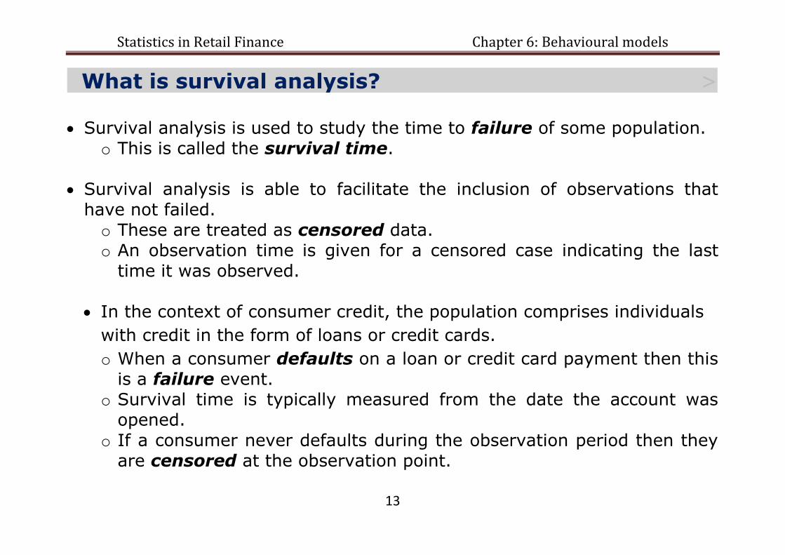
What is survival analysis? >

Survival analysis is used to study the time to failure of some population.

o This is called the survival time.

Survival analysis is able to facilitate the inclusion of observations that

have not failed. o These are treated as censored data. o An observation time is given for a censored case indicating the last

time it was observed.

In the context of consumer credit, the population comprises individuals

with credit in the form of loans or credit cards.

o When a consumer defaults on a loan or credit card payment then this is a failure event.

o Survival time is typically measured from the date the account was opened.

o If a consumer never defaults during the observation period then they are censored at the observation point.


14

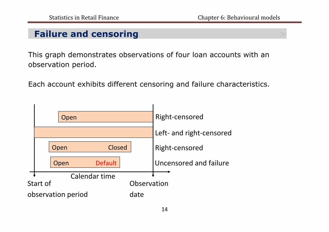
Failure and censoring >

This graph demonstrates observations of four loan accounts with an

observation period.

Each account exhibits different censoring and failure characteristics.

Open

Open Closed

Open Default

Start of

observation period

Observation

date

Calendar time

Right-censored

Left- and right-censored

Right-censored

Uncensored and failure


15

Hazard Function >

A common means to analyze survival data is through the hazard function which gives the instantaneous chance of failure at time t:

t

tTttTtPth

t

|lim)(

0

where T is a random variable associated with survival time.

In consumer credit, several studies demonstrate the classic shape for

default hazard as:-

Highest risk of default is within the first few months, then the risk tails off over the lifetime of the loan or credit card.


16

Example 6.3

Hazard rates for Default on a Store Card.

95% confidence intervals on the estimate are also shown

(Andreeva, Ansell, Crook 2007).

0

0.002

0.004

0.006

0.008

0.01

0.012

0.014

0.016

1 3 5 7 9 11 13 15 17 19 21 23

H

a

z

a

r

d

Time (months)


17

Probability of Default >

The survival probability at time t can be given in terms of the hazard

function:

This is the probability of survival from time 0 to some time t.

For credit data, this gives the probability of default (PD) as:-


18

The survival probability is related to the hazard function, since

)(

)(lim

|lim)(

00 tS

tftTP

t

ttTtP

t

tTttTtPth

tt

where is the probability density function of .

Since , where is the cumulative distribution function on ,

Therefore, integrating over , substituting ,

∫

∫

[ ]

since . Therefore,

( ∫

)


19

Cox Proportional Hazards Model >

There are several alternative survival models to estimate the hazard function.

We will look at perhaps the most popular in the credit scoring literature: The Cox Proportional Hazards (PH) model.

Named after Sir David Cox

(Professor of Statistics at Imperial College London from 1966 to 1988).

The Cox PH model allows us to model survival in terms of the borrower

characteristics. In particular, the hazard function changes with the values of

predictor variables.


20

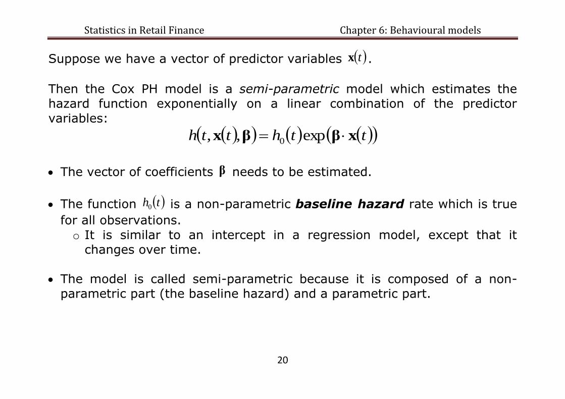
Suppose we have a vector of predictor variables tx .

Then the Cox PH model is a semi-parametric model which estimates the hazard function exponentially on a linear combination of the predictor

variables:

tthtth xββx exp,, 0

The vector of coefficients β needs to be estimated.

The function th0 is a non-parametric baseline hazard rate which is true

for all observations.

o It is similar to an intercept in a regression model, except that it changes over time.

The model is called semi-parametric because it is composed of a non-parametric part (the baseline hazard) and a parametric part.


21

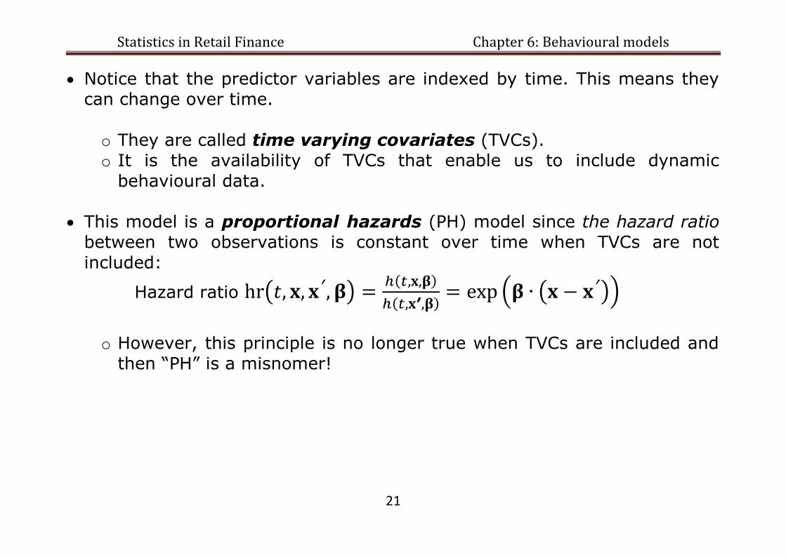
Notice that the predictor variables are indexed by time. This means they can change over time.

o They are called time varying covariates (TVCs). o It is the availability of TVCs that enable us to include dynamic

behavioural data.

This model is a proportional hazards (PH) model since the hazard ratio between two observations is constant over time when TVCs are not

included:

Hazard ratio ( )

( ( ))

o However, this principle is no longer true when TVCs are included and

then “PH” is a misnomer!


22

Partial likelihood function > The Cox PH model is estimated using maximum likelihood estimation (MLE) based on a training data set.

Suppose we have n observations for i=1 to n:

observation times ti

indicator variables ci where

o ci=0 for a censored observation and

o ci=1 for a failure event (default);

if ci=1 then ti is the survival time,

predictor variable values xi(t).

The baseline hazard complicates the likelihood function.

Therefore the likelihood function is decomposed into two components:

1. The probability that a failure event occurs at a time ; 2. The probability that it was a specific observation i that failed at time ,

given that a failure occurred.


23

It turns out that using just the second component is sufficient to get estimates of β .

This is called partial likelihood estimation.

The practical effect is that partial likelihood estimates have higher standard errors than using MLE.

The probability that an observation fails at some time t, amongst all other

observations is therefore given by

)()(

)(exp

)(exp

,,

,,

tRj

j

i

tRj

j

i

t

t

tth

tth

xβ

xβ

βx

βx

where R(t) is called the risk set and includes all observations that are

uncensored and have not failed by time t.

Specifically, ttjtR j )(:)( where )( jt are ordered survival times.


24

Partial likelihood function >

This gives the partial likelihood function for the Cox PH model:

n

i

c

tRj

ij

ii

p

i

i

t

tl

1

)(

)(

)(

)(

)(exp

)(exp)(

xβ

xββ

Maximizing this with respect to β gives an estimate of β .

Typically the Cox PH model is used as an explanatory model, in which case

an estimate of is sufficient.


25

Forecasting survival probability > For retail finance, we are primarily interested in forecasting the survival

function for an individual, , since this is related to the PD, . For forecasting, the baseline hazard will also need to be estimated. A nonparametric MLE is used to do that, based on the initial estimate of .

In the survival setting, for forecasting, an estimate of the survival curve is required for each observation. Since, in general, for the Cox PH model,

( ∫

) ( ∫ ( )

)

it follows for each observation an estimate is given by

( ∫ ( )

)

Notice that an estimate of is needed.


26

Estimating the baseline hazard >

There are different ways to estimate , but one approach that has been

suggested is to estimate the cumulative baseline hazard

∫

∑

∑ ( ( )) ( )

Then

for some appropriately small .

Since the formula for includes an integral, in practice, the estimation of

survival probability requires a numerical integration method, if TVCs are

included.


27

However, if no TVCs are included in the model, so for all ,

( ( ))

which does not require numerical integration.

Indeed, many statistical packages, such as R and SAS, have standard

functions to estimate the baseline hazard and survival probability when

no TVCs are in the model, but they do not work if TVCs are included.


28

Behavioural models using survival models > It is straightforward to include behavioural variables directly as TVCs.

However, for the models to be useful for forecasting, it is necessary that they are entered with a lag in relation to outcome.

That is, if survival time is t, then behavioural data from time t-k is

included, for some lag time k.

This means we can forecast outcome for some time k ahead.


29

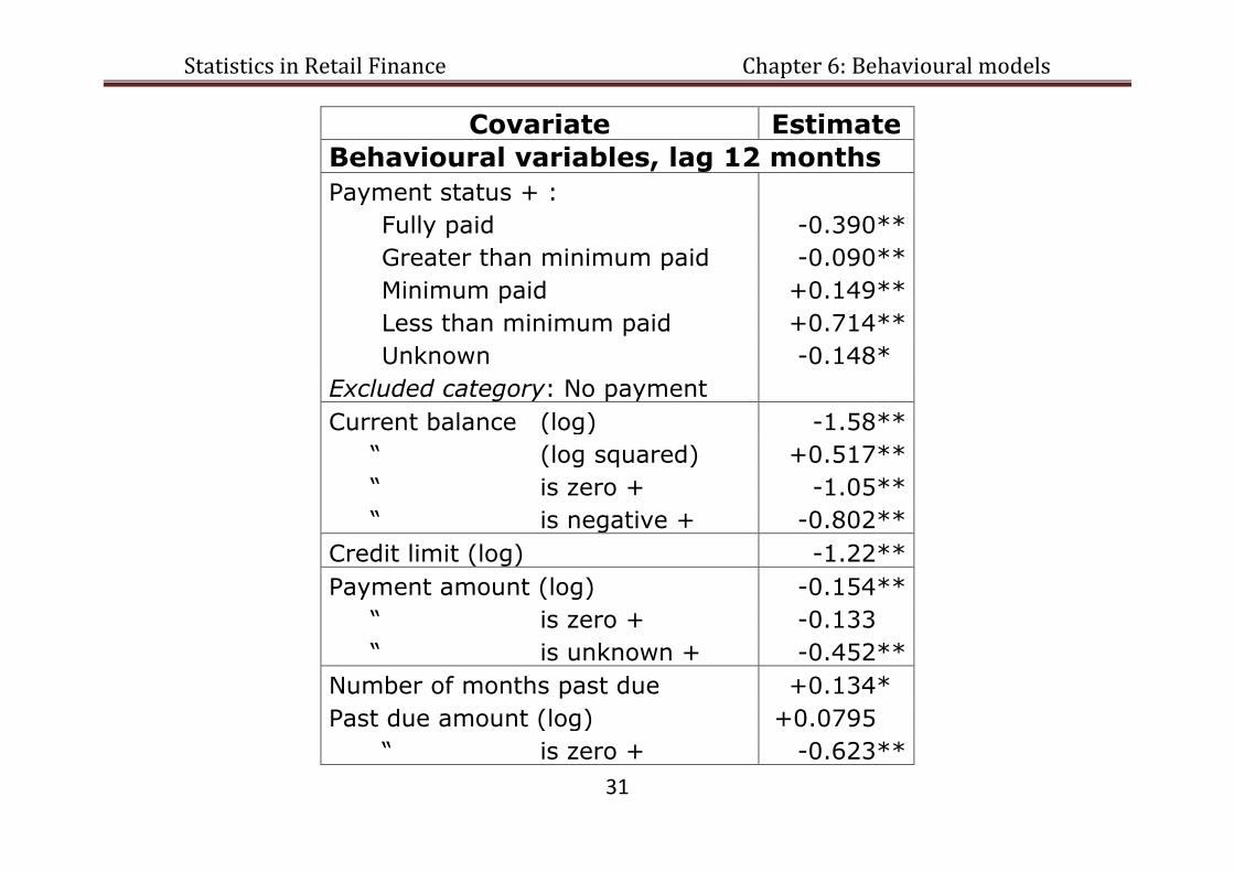
Example 6.4

A behavioural model with default as failure event for a credit card data set ( ).

Coefficient estimates for a model with fixed application variables (AV) and

time varying monthly behavioural variables (BV). Indicator variables are denoted by a plus sign (+).

Statistical significance levels are denoted by asterisks:

** is less than 0.001 and

* is less than 0.01 level.

Covariate Estimate

Selected AVs:

Time customer with bank (years) -0.00250 **

Income (log) -0.146 **

Number of cards -0.0610 **

Time at current address -0.00129


30

Covariate Estimate

Employment + :

Self-employed +0.303 **

Homemaker +0.072

Retired +0.111

Student -0.035

Unemployed +0.231

Part time -0.365 **

Other -0.037

Excluded category: Employed

Age + : 18 to 24 +0.074

25 to 29 -0.058

30 to 33 +0.010

34 to 37 +0.100 **

38 to 41 +0.046

48 to 55 -0.108 **

56 and over -0.243 **

Excluded category: 42 to 47

Generic credit score -0.00322 **


31

Covariate Estimate

Behavioural variables, lag 12 months

Payment status + :

Fully paid -0.390 **

Greater than minimum paid -0.090 **

Minimum paid +0.149 **

Less than minimum paid +0.714 **

Unknown -0.148 *

Excluded category: No payment

Current balance (log) -1.58 **

“ (log squared) +0.517 **

“ is zero + -1.05 **

“ is negative + -0.802 **

Credit limit (log) -1.22 **

Payment amount (log) -0.154 **

“ is zero + -0.133

“ is unknown + -0.452 **

Number of months past due +0.134 *

Past due amount (log) +0.0795

“ is zero + -0.623 **


32

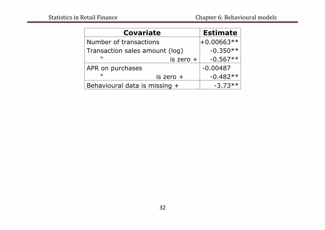
Covariate Estimate

Number of transactions +0.00663 **

Transaction sales amount (log) -0.350 **

“ is zero + -0.567 **

APR on purchases -0.00487

“ is zero + -0.482 **

Behavioural data is missing + -3.73 **


33

Example 6.4 continued

Forecasting using survival models with BVs, using a Deviance model fit measure.

Forecasts of time to default improve with the inclusion of BVs and shorter lag time.

Of course, a shorter lag implies a shorter period to forecast ahead.

120000

130000

140000

150000

160000

AV o

nly

AV &

BV

lag 1

2

AV &

BV

lag 9

AV &

BV

lag 6

AV &

BV

lag 3

Model

-Log-lik

elih

ood .

35000

40000

45000

50000

55000

Devi

ance

.

Model fit: - log likelihood ratio Forecast: Deviance residual


34

Exercise 6.1

Interpret the association of each of these behavioural variables with the default hazard rate in the model given in Example 17.1:-

Payment status Current balance Credit limit Number of months past due

Number of transactions Transaction sales amount


35

Exercise 6.2

a) Let be the hazard function at time . Show that the survival

probability is given by ( ∫

).

b) A hazard function for default is given by

{

for some and . Suppose we want to ensure probability of

default at time is less than a given value and is fixed. Then, what is

the inequality constraint on ?


36

c) Interpret the following Cox Proportional Hazards model of time to default:

i. Which are the statistically significant variables at a 1% level? ii. What effect does each variable have on default hazard risk?

Predictor variable Range of values Coefficient Estimate

P-value

Employment status at application

1 (yes) or 0 (no) -0.50 0.001

Generic credit score 0 to 999 -0.004 0.002

Current balance (log), lag 6 months

0 to 6 +0.20 0.121

Payment missed, lag 6 months

1 (yes) or 0 (no) +1.20 0.001


37

References for Survival models > Hosmer Jr. DW and Lemeshow S (1999). Applied Survival Analysis:

regression modelling of time to event data. Wiley.

Andreeva, G., Ansell, J., Crook, J. N. (2007). Modelling Profitability using Survival Combination Scores, European Journal of Operational

Research (published by Elsevier) There are actually many other good text books on Survival modelling.

http://webdb.ucs.ed.ac.uk/management/msm/research/publications/vie_dets.cfm?artID=4195

http://webdb.ucs.ed.ac.uk/management/msm/research/publications/vie_dets.cfm?artID=4195


38

Markov transition models > We now move on to a new dynamic model structure…

Markov transition models (or Markov chains) are a dynamic approach to modelling processes with changes of state.

They are valuable in credit scoring since they allow us to model changes in the state of an account over time. For instance,

Modelling the number of account periods of delinquency. Changes in behavioural score.

Markov transition models are especially useful for modelling revolving credit

with highly variable credit usage.

For instance, for tracking credit card use.


39

First-order Markov transition model > Some definitions:

Let be a sequence of random variables taking values from { } for some fixed .

The sequence is a finite-valued first-order Markov chain if

for all and , such that and .

We denote and call this the transition

probability. o The transition probability represents the probability of moving

from one state to another state .

The transition matrix is defined as a matrix such that [ ] .


40

If we make a prior assumption that a transition from state to state in

the th period then we fix and call this a structural zero.

A Markov chain is stationary if for all for some transition matrix

. That is, the transition probabilities are the same over all periods.

Notice that

∑

∑

∑

by the law of total probability and first-order Markov chain assumption.


41

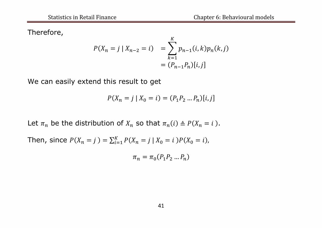
Therefore,

∑

[ ]

We can easily extend this result to get

[ ]

Let be the distribution of so that . Then, since ∑


42

Example 6.5

Consider a two state stationary Markov chain for behavioural score change (state 1=high score, 2=low score) with transition matrix

(

)

Suppose we start with an individual having high score. What are the distributions after one and two periods?

Solution

Therefore, after one period:

(

)

And, after two periods,

(

)


43

Estimation of the transition matrix > Use maximum likelihood estimation (MLE) for each .

Given a sequence of realizations , the probability of this

realization is given as

(∏

)

∏

∏


44

Therefore, the log-likelihood function is

∑

∑∑

where { } .

However, the likelihood function is constrained by ∑

Therefore, choose some such that and substitute

∑

{ } { }

to get

∑[( ∑

{ } { }

) ( ∑

{ } { }

)]


45

Then find the derivative with respect to each where and set to

zero to find the maxima:

Therefore,

But, the choice of is arbitrary so for consistency the result must hold

generally for all . In particular, the MLE is

∑

Notice that this result easily generalizes to the case when we have multiple sequences of realizations (eg more than one borrower), so long as we assume independence between each sequence.


46

Example 6.6

Consider three states (1=high score, 2=low score, 3=default) for a stationary process. Transition probabilities are given as: from a high score to a low score is 0.05;

from a low score to a high score is 0.1; from a low score to default is 0.02.

It is impossible to move from high score to default. Also, it is impossible to move out of default.

1. What is the transition matrix? 2. How many structural zeroes are there in the matrix?

Solution

(

)

There are 3 structural zeroes.


47

Extensions to Markov transition models >

An obvious omission from the Markov chain formulation is the lack of

predictor variables.

There are two ways to include borrower details in the model:

1. Include behavioural variables within the state space.

2. Segment the population on static variables and build segmented

Markov transition models.


48

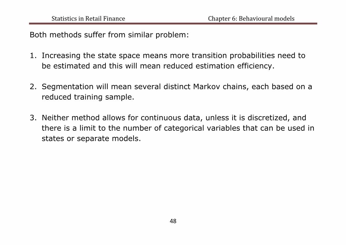
Both methods suffer from similar problem:

1. Increasing the state space means more transition probabilities need to

be estimated and this will mean reduced estimation efficiency.

2. Segmentation will mean several distinct Markov chains, each based on a

reduced training sample.

3. Neither method allows for continuous data, unless it is discretized, and

there is a limit to the number of categorical variables that can be used in

states or separate models.


49

Example 6.7

Suppose we want to include credit usage, in terms of monthly spend in a

model for behavioural score (Low or High).

First discretize credit usage into levels:

eg three levels: monthly spend < £200, £200 and < £1000, £1000,

Then, form 6 states, instead of 2:

Behavioural score Monthly spend State

Low < £200 1

Low £200 and < £1000 2

Low £1000 3

High < £200 4

High £200 and < £1000 5

High £1000 6


50

Example 6.8

Research suggests two broad categories of credit card usage: the movers

and stayers.

Movers are those whose credit card usage is erratic; having periods of

heavy credit card usage then quiet periods.

Stayers, by contrast, tend to be steady, and stay in the same state

over long periods.

We could build a static behavioural model to broadly categorize borrowers

into one of the two categories.

Then separate Markov transition models could be built separately for the

two segments.


51

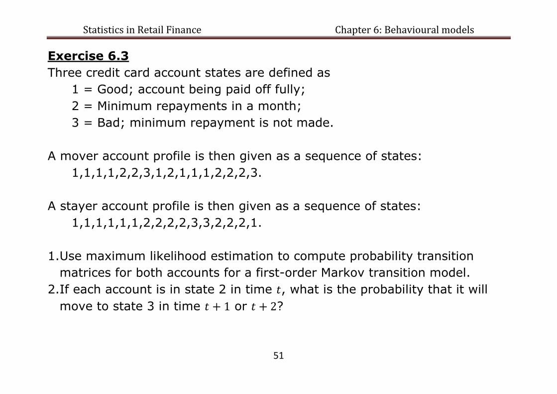
Exercise 6.3

Three credit card account states are defined as

1 = Good; account being paid off fully;

2 = Minimum repayments in a month;

3 = Bad; minimum repayment is not made.

A mover account profile is then given as a sequence of states:

1,1,1,1,2,2,3,1,2,1,1,1,2,2,2,3.

A stayer account profile is then given as a sequence of states:

1,1,1,1,1,1,2,2,2,2,3,3,2,2,2,1.

1.Use maximum likelihood estimation to compute probability transition

matrices for both accounts for a first-order Markov transition model.

2.If each account is in state 2 in time , what is the probability that it will

move to state 3 in time or ?


52

Roll-rate model >

A roll-rate model is a type of Markov transition model but the focus is on the

number of accounts or value of loans that rolls over from one level of

delinquency to another over several months.

Consider states where 0 corresponds to no delinquency, states >0

correspond to increasing levels of delinquency and corresponds to

loan default with write-off.

Let be a vector of initial number of accounts or value of loans.

Let be a transition matrix.

Then the vector of values in each state at month t is given by .


53

Example 6.9

Let .

Let , in GB£.

Let (

).

Let first month ( ) be January 2013.

Then roll-rate table (projection) for six months is computed as:-

Month Computation State

0 1 2 3

Jan 13 50000 10000 5000 1000

Feb 13 52500 5250 5750 2500

Mar 13 53600 3438 4737 4225

Apr 13 54033 2684 3637 5646

May 13 54121 2336 2805 6737

Jun 13 54020 2157 2244 7579


54

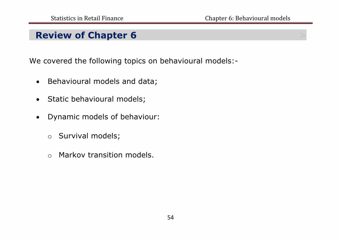
Review of Chapter 6 >

We covered the following topics on behavioural models:-

Behavioural models and data;

Static behavioural models;

Dynamic models of behaviour:

o Survival models;

o Markov transition models.

Statistics in Retail Finance Chapter 6: Behavioural...

Documents

Transcript of Statistics in Retail Finance Chapter 6: Behavioural...