Statistics for Retail Finance Chapter 8: Regulation …bm508/teaching/retailfinance/Lecture8.pdf ·...

Statistics for Retail Finance Chapter 8: Regulation and Capital Requirements

1

Statistics for Retail Finance

Chapter 8: Regulation and Capital Requirements


2

Overview >

We now consider regulatory requirements for managing risk on a portfolio of

consumer loans.

Regulators have two key duties:

1. Protect consumers in the financial market place.

2. Provide the means for a stable and efficient financial market.

Lenders must ensure they have sufficient capital to cover possible losses on

a portfolio of loans. This is their capital requirement.


3

How much is a sufficient capital requirement?

Well, the banks could cover every £1 lent with £1 of cash.

o However, that would be an expensive and impractical solution.

The usual solution is to cover some percentage of the loan value on the

grounds that only a small percentage of the loans will go bad.

o A usual figure in the past has been to have 8% of loan value as

capital reserve.

o This is a risk, however, since it is possible to under-estimate the

number of bad loans.

o Now, however, capital requirement is calculated based on measuring

the risk of a portfolio of loans.


4

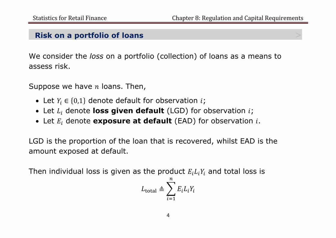
Risk on a portfolio of loans >

We consider the loss on a portfolio (collection) of loans as a means to

assess risk.

Suppose we have loans. Then,

Let { } denote default for observation ;

Let denote loss given default (LGD) for observation ;

Let denote exposure at default (EAD) for observation .

LGD is the proportion of the loan that is recovered, whilst EAD is the

amount exposed at default.

Then individual loss is given as the product and total loss is

∑


5

To understand risk, we need to develop a distribution for an estimate of

total loss. This is not easy since separate models for each of the three

components are required along with an understanding of their correlations:

Default models are well-understood.

However, models of LGD and EAD are still being developed.

Although there is some evidence of a correlation between LGD and

default, the size of the correlation is still not well-understood.


6

Expected Loss with fixed EAD and LGD >

For this reason, often the loss is simplified by taking EAD and LGD as

constant for all loans.

Therefore, for all , we assume , for some fixed values.

Define the default rate as

∑

Then, total loss is given by

and expected loss (EL) on an individual is

( )

where ( ) is the probability of default (PD) for observation .


7

In the credit risk literature, this is usually written as

Expected Loss = PD LGD EAD

EL on a portfolio (collection) of loans is then given by

( ) ( ) ( )

where

( )

∑

Therefore, EL can be computed using just a model of default, and PDs can

be taken from a calibrated scorecard (eg using log-odds scores).


8

Variance of Default Rate >

The EL does not tell us about the risk. Traditionally, in portfolio

management, it is the variance that tells us about risk.

We can compute variance on Default Rate:

( ) ((

∑

)

) ( ( ))

(∑

∑∑

) (

∑

)

[∑ ( ) ∑

∑∑( ( ) )

]

since .


9

Therefore

( )

[∑ ( )

∑∑

]

where ( ).

If we assume no covariance between observations, then this allows us to

easily compute variance.

However, this is not a reasonable assumption since defaults are likely to be

correlated with each other.

So we need to be able to estimate the covariance structure.


10

Value at Risk >

Although variance gives a measure of risk, what is of most interest to

lenders and regulators is that lenders can cover a large proportion of

possible losses and in particular the extreme losses that might be

experienced during a recession.

For this reason, in credit risk management the focus is on estimating an

upper quantile of the loss distribution.

In Finance, this is known as the Value at Risk (VaR).

Let be a cumulative distribution function on loss .

Then, for a percentage ( ),

( ) ( )

Typical VaR are estimated at 99% or 99.9% levels.


11

So, VaR(99%) gives us an upper bound on 99% of possible losses.

Therefore, it will only underestimate loss in 1% of cases.

Please do not confuse VaR with Variance!


12

Example 8.1

This graph illustrates the loss distribution.

It shows Expected Loss (EL) and VaR (99% level).

VaR can be much larger

than EL, especially when

the loss distribution has a

long right tail (this is

usual).

0 5 10 15 20

Loss (in £ million)

Loss distribution Expected Loss VaR(99%)


13

Economic and Regulatory Capital >

Economic capital is the capital a bank deems necessary to run its

business. It will cover the Expected Loss, whilst allowing for unusually high

losses. This is a matter for internal bank policy.

Regulatory capital (RC) is the capital that regulators believe the banks

need to keep against unexpected losses. There may be a cross-over with

economic capital, but the calculation of RC is imposed by financial

regulators.

Each country has its own regulatory authority (eg Federal Reserve in the

USA and Financial Services Authority in the UK).

However, most countries now follow the Basel III rules set out by the

Bank for International Settlements (BIS) in Switzerland.


14

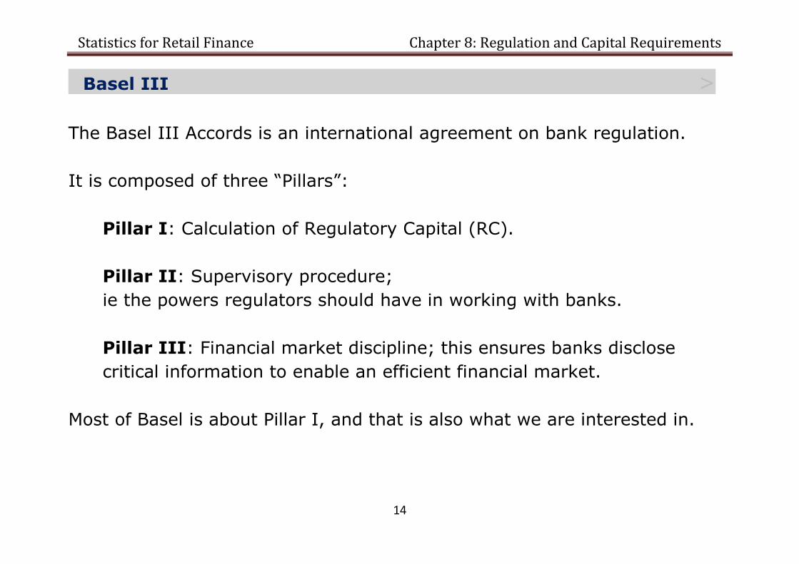
Basel III >

The Basel III Accords is an international agreement on bank regulation.

It is composed of three “Pillars”:

Pillar I: Calculation of Regulatory Capital (RC).

Pillar II: Supervisory procedure;

ie the powers regulators should have in working with banks.

Pillar III: Financial market discipline; this ensures banks disclose

critical information to enable an efficient financial market.

Most of Basel is about Pillar I, and that is also what we are interested in.


15

Basel III Regulatory Capital (Pillar I) >

Basel III allows banks to calculate RC in one of three ways.

Standard approach;

Internal-ratings based (IRB) approach: foundational;

Internal-ratings based (IRB) approach: advanced.

The standard approach follows the traditional method of setting RC as a

percentage of loan amount (Basel I). However, it is not quite so simplistic

since different types of loans require a different percentage to be set aside

based on risk levels of the loan type.

Both IRB approaches allow banks to use their own risk models to

determine RC. This is attractive since it allows knowledge about a specific

credit product to inform the RC computation. Since models of default are so

well-established in the industry, both approaches require banks to provide


16

estimates of PD. However, since LGD is less well-understood, the

foundational approach allows banks to use a fixed value of LGD provided

by the regulator. Additionally both approaches allow banks to use an

estimated value for EAD.

To summarize:

RC approach Bank estimate required?

PD LGD EAD

Standard No No No

IRB foundational Yes No May be used

IRB advanced Yes Yes Yes

The major banks have chosen to use one of the IRB approaches.


17

Basel IRB Regulatory Capital calculation >

In Basel III, RC is simply calculated as the difference between the VaR and

EL. It therefore covers all “unexpected losses”; ie losses that could occur in

extreme conditions. Therefore,

( ) ( )

Note that ( ) is expected to be covered by provisioning and pricing of

the credit product by the lender.

We can easily compute ( ), but a loss distribution is required to

compute VaR.

o As we have seen, this is a problem since we need to estimate the

correlation structure between default events.


18

One Factor Model >

We cannot realistically model all possible correlations between accounts.

Instead, we assume portfolio invariance;

ie that there is one factor that governs the correlation between default

events.

Additionally, we use Merton’s (1974) assumption:

A borrower will default if the borrower’s assets fall below the value of

debts.

Suppose we want to measure risk of default for an individual over a period

of time. For each borrower ,

Let be the fixed debt over that period.

Let be fixed assets at the start of the period.

Let be a random variable representing assets at the end of the

period.


19

Assume that the difference in asset values is normally distributed:

( )

Then model this difference using a one factor model

where

( ) is a common systematic factor, scaled by and

( ) is an idiosyncratic factor scaled by ,

such that and are independent and the ’s are independent,

and .

This is known as a Merton-type model.


20

Notice that this model assumes that changing assets is associated with a

combination of

A common systematic factor ; and

An idiosyncratic factor which depends on the individual.

The common factor represents changing economic or social conditions which

are universal to everyone in the loan portfolio.


21

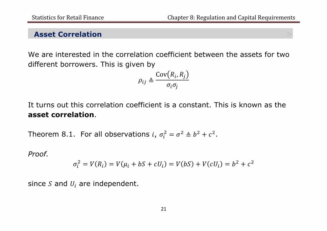
Asset Correlation >

We are interested in the correlation coefficient between the assets for two

different borrowers. This is given by

( )

It turns out this correlation coefficient is a constant. This is known as the

asset correlation.

Theorem 8.1. For all observations , .

Proof.

( ) ( ) ( ) ( )

since and are independent.


22

Theorem 8.2. For all observations and such that ,

Proof.

( ) (( )( )) ( ) ( )

( ) ( )

since ( ) , ( ) and and are independent.

Therefore, ( ) , since each and are independent.

The result then follows using Theorem 1.


23

PD in Merton’s Model >

Remember Merton’s assumption:

A borrower will default if assets fall below the value of debts.

We can now use this to estimate PD. It is the probability that assets at the

end of the period are less than the debt:

( ) ( ) (

)

(

)

where is the cumulative standard normal distribution, since ( ).


24

Conditional PD >

PD is then derived conditional on the value of factor :

( ) ( ) ( )

(

)

(

)

( ( ) √

√ )

Notice this is a latent variable model, since values of are not actually

needed to extract PD.


25

Loss Distribution on PD >

The loss distribution on PD is then constructed on the random variable

( ).

All that is needed to get a specific loss distribution is

1. An estimate of “usual” PD;

We can use a standard scorecard model to do that, and

2. An estimate of the asset correlation .

In Basel III, VaR is computed at the 99.9% level (so RC is underestimated

with only a 1/1000 chance).

We adjust to account for that.

Larger is linked to higher assets, therefore we take the lowest 0.1

percentile.

Since ( ), this is ( )

( ).


26

Therefore, the VaR on PD at 99.9% is

(

( )) ( ) ( ( )

( )√

√ )

Basel II also specifies asset correlations. For instance,

=0.04 for revolving credit;

=0.15 for residential loans.

These asset correlations have been estimated based on historic data.

By considering loss at the individual level, if we fix LGD and EAD, RC is then

given by

( ) ( )

( ( ) )


27

Example 8.2

The following graph shows the shape of RC, per unit of EAD, with

LGD=0.75.

So, for instance, if a

residential loan has

PD=0.02, then

RC=£0.117 for every £1

of the loan.

0

0.1

0.2

0.3

0.4

0 0.2 0.4 0.6 0.8 1

RC

(p

er

un

it o

f EA

D)

PD

Revolving credit Residential loans


28

Criticism of Merton-type models for consumer credit >

There have been several criticisms of the Merton model as used in consumer

credit.

1. The Merton model was originally designed for corporate loans. In that

context it makes sense. It was used for consumer loans because no

satisfactory alternative models were available for consumer credit.

2. The Merton assumption may not apply in consumer credit. Do all

borrowers wait until asset value falls below debt before defaulting? In

particular, many defaulters are those that simply won’t pay, even if

they have assets. Indeed, evidence suggests that for individuals

(rather than corporation) cash-flow affects default, rather than overall

assets.

3. Estimates of asset correlation have been criticized. It is not clear how

they have been estimated, and it is suggested they have been set too

high.


29

Exercise 8.1

In the usual one factor model for consumer credit, difference in assets for

a borrower is modelled by

where ( ) is a common factor scaled by , ( ) is an idiosyncratic

factor scaled by , and and are independent and the ’s are all

independent.

a) Show that the correlation coefficient between difference in assets

and for two borrowers and is ⁄ for all and such that

, where .

Suppose the one factor model is modified so that there is a fixed correlation

between the idiosyncratic factors. That is, the correlation coefficient

between and for all and such that is given by .


30

b) Show that with this modification, the correlation coefficient between

difference in assets and for two borrowers and is

for all and such that .

c) Express the probability of default (PD) conditional on the realization of

, ( ), in terms of the unconditional PD ,

, and .

d) Fixing values of , and , describe the effect of different values of

[ ] on

( ). In particular, what is ( ) at the extremes of the

range: and ?


31

Stress Testing >

In Pillar II, regulators also have powers to stress test banks, to determine

how they will respond to extreme recessionary circumstances.

Regulators expect banks to be able to survive extreme, but plausible,

economic conditions.

There are three general approaches to stress testing:

1. Analytic: Use a parametric loss distribution to compute extreme risk;

2. Scenarios: Either historic scenarios or designed by economists;

3. Simulation: Based on a dynamic model of default.


32

The 2nd and 3rd approach both rely on models that allow inclusion of

extreme conditions to determine how this changes Expected Loss.

For example, a survival model of default could be built with

macroeconomic variables as time varying covariates (TVCs). Then risk

of default is then a function of macroeconomic conditions.

The scenario approach (2nd) produces one point estimate of effect on

Expected Loss for each scenario.

The simulation approach (3rd) will use Monte Carlo simulation to

generate a distribution of Expected Loss based on a multivariate

distribution of plausible economic scenarios.

The scenario approach has the advantage that it reflects realistic

historical conditions. The simulation approach, however, is able to take

account of plausible but not historic conditions.

Something to think about: Is one economic crisis just like another????


33

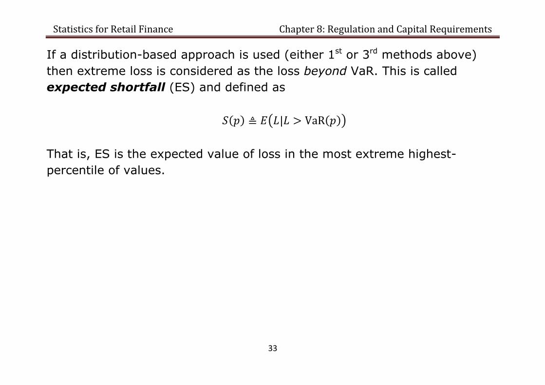
If a distribution-based approach is used (either 1st or 3rd methods above)

then extreme loss is considered as the loss beyond VaR. This is called

expected shortfall (ES) and defined as

( ) ( ( ))

That is, ES is the expected value of loss in the most extreme highest-

percentile of values.


34

This graph shows the loss distribution with scenarios and ES also included.

0 5 10 15 20

Loss (in £ million)

Loss distribution Expected Loss VaR(99%)

ES(99%) region ES(99%) Scenarios


35

Example 8.3

The FSA has published an ‘anchor’ scenario which can be used for stress

testing. It specifies a series of economic conditions over a period of years of

a recession. Therefore, a bank would need to determine how their portfolio

of loans would behave over those years.

Unemployment GDP CRE HPI FTSE

All-Share

Year 1 8.9 -2.1 -21.7 -10.1 -18.7

Year 2 10.3 -3.0 -18.5 -11.3 -7.0

Year 3 11.3 -0.1 -3.8 -7.1 3.8

Year 4 11.0 1.4 -0.8 -0.7 3.7

Year 5 10.3 1.8 -4.3 0.4 -5.9

CRE = Commercial Real Estate and HPI = House Price Index

Note: Values for GDP, CRE, HPI and FTSE represent annual change.

Source: www.fsa.gov.uk. These figures are correct as of January 2013.

http://www.fsa.gov.uk/


36

Review of Chapter 8 >

We have covered the following topics on regulation and capital

requirements.

Capital Requirements

Loss Distribution

Value at Risk

Basel III Accord

One Factor / Merton Model

Stress Testing

Statistics for Retail Finance Chapter 8: Regulation …bm508/teaching/retailfinance/Lecture8.pdf ·...

Documents

Transcript of Statistics for Retail Finance Chapter 8: Regulation …bm508/teaching/retailfinance/Lecture8.pdf ·...