Statistics for Experimental Economists
245
Statistics Statistics for for Experimental Experimental Economists Economists elegant analysis with R elegant analysis with R Mark A. Olson File book.tex, last update 2014/07/17, version 0.6.4743
Transcript of Statistics for Experimental Economists

StatisticsStatistics
forfor
ExperimentalExperimental
EconomistsEconomists
elegant analysis with Relegant analysis with R
Mark A. Olson
File book.tex, last update 2014/07/17, version 0.6.4743

Copyright © 2014 Mark A. Olson
Published by EREHWONE Publishers
statistics.experimentalecon.org
First printing, September 2014


Contents
Contents iv
List of Figures x
Preface xiii
I One 1
1 Introduction 2
1.1 Why a Special Book? . . . . . . . . . . . . . . . . . . . . . . . . . . 2
1.2 Partial Outline . . . . . . . . . . . . . . . . . . . . . . . . . . . . . 3
2 The Tao of Research 5
2.1 The Problem of Scientific Inference . . . . . . . . . . . . . . . . . . 5
2.2 Deduction . . . . . . . . . . . . . . . . . . . . . . . . . . . . . . . . 8
2.3 Induction . . . . . . . . . . . . . . . . . . . . . . . . . . . . . . . . . 8
2.4 Causality . . . . . . . . . . . . . . . . . . . . . . . . . . . . . . . . . 9
2.5 Confounding . . . . . . . . . . . . . . . . . . . . . . . . . . . . . . . 10
2.6 Randomization . . . . . . . . . . . . . . . . . . . . . . . . . . . . . 10
3 What is an Experiment 19
3.1 Causality, Correlation, Independence . . . . . . . . . . . . . . . . . 20
3.2 Background . . . . . . . . . . . . . . . . . . . . . . . . . . . . . . . 20
3.3 Causality and nonrandomized research . . . . . . . . . . . . . . . . 21
iv

CONTENTS v
3.4 Does Correlation Imply Causation . . . . . . . . . . . . . . . . . . . 21
3.5 Independence and Correlation . . . . . . . . . . . . . . . . . . . . . 22
3.6 Natural Experiments . . . . . . . . . . . . . . . . . . . . . . . . . . 22
4 Zen of economic experiments 24
4.1 Description . . . . . . . . . . . . . . . . . . . . . . . . . . . . . . . . 24
4.2 Types of economic experiments . . . . . . . . . . . . . . . . . . . . 25
4.3 Early Experiments . . . . . . . . . . . . . . . . . . . . . . . . . . . 26
4.4 Randomization in Economic Experiments . . . . . . . . . . . . . . . 27
4.5 Experimental Bias . . . . . . . . . . . . . . . . . . . . . . . . . . . . 27
4.6 Repeating Trials . . . . . . . . . . . . . . . . . . . . . . . . . . . . . 27
4.7 Replications . . . . . . . . . . . . . . . . . . . . . . . . . . . . . . . 29
4.8 Structure of the Economic Experiment . . . . . . . . . . . . . . . . 29
5 Experimental Model 30
5.1 Model dependent inference . . . . . . . . . . . . . . . . . . . . . . . 30
5.2 Probability Models . . . . . . . . . . . . . . . . . . . . . . . . . . . 31
5.3 Models . . . . . . . . . . . . . . . . . . . . . . . . . . . . . . . . . . 31
6 Design Choices and Design Problems 32
6.1 The Design . . . . . . . . . . . . . . . . . . . . . . . . . . . . . . . . 33
6.2 Fundamental assumptions of experimental design . . . . . . . . . . 33
6.3 Experimental design . . . . . . . . . . . . . . . . . . . . . . . . . . 33
6.4 Data Pooling and Simpson’s Paradox . . . . . . . . . . . . . . . . . 39
6.5 Regression Toward the Mean . . . . . . . . . . . . . . . . . . . . . . 44
6.6 Regression Fallacy . . . . . . . . . . . . . . . . . . . . . . . . . . . . 44
6.7 The Ecological Fallacy . . . . . . . . . . . . . . . . . . . . . . . . . 45
7 Preliminaries 46
7.1 Types of Data . . . . . . . . . . . . . . . . . . . . . . . . . . . . . . 46
7.2 Experimental Terms . . . . . . . . . . . . . . . . . . . . . . . . . . . 49
7.3 Types of Analysis . . . . . . . . . . . . . . . . . . . . . . . . . . . . 52
7.4 Statistical Testing . . . . . . . . . . . . . . . . . . . . . . . . . . . . 54
7.5 How are We to Judge Which Test to Use? . . . . . . . . . . . . . . 54
8 Hypothesis Testing and Significance 57
8.1 What is Hypothesis Testing? . . . . . . . . . . . . . . . . . . . . . . 57
8.2 Null Hypothesis . . . . . . . . . . . . . . . . . . . . . . . . . . . . . 59
8.3 Hypothesis Testing Assumptions . . . . . . . . . . . . . . . . . . . . 59
8.4 Probability Models . . . . . . . . . . . . . . . . . . . . . . . . . . . 61
8.5 Randomization Model . . . . . . . . . . . . . . . . . . . . . . . . . . 62

CONTENTS vi
8.6 Alpha . . . . . . . . . . . . . . . . . . . . . . . . . . . . . . . . . . . 63
8.7 P-value . . . . . . . . . . . . . . . . . . . . . . . . . . . . . . . . . . 63
8.8 Problems with Hypothesis Testing . . . . . . . . . . . . . . . . . . . 64
8.9 Confidence Intervals . . . . . . . . . . . . . . . . . . . . . . . . . . . 65
8.10 Practical vs. Statistical Significance . . . . . . . . . . . . . . . . . . 65
8.11 Wald Missing Data example . . . . . . . . . . . . . . . . . . . . . . 65
8.12 One or Two Sided Tests? . . . . . . . . . . . . . . . . . . . . . . . . 65
8.13 Multiple Testing . . . . . . . . . . . . . . . . . . . . . . . . . . . . . 70
8.14 Applying More Than One Test . . . . . . . . . . . . . . . . . . . . . 71
8.15 Power of Test . . . . . . . . . . . . . . . . . . . . . . . . . . . . . . 72
8.16 Power and Effect Size . . . . . . . . . . . . . . . . . . . . . . . . . . 73
8.17 Power for Binomial Example . . . . . . . . . . . . . . . . . . . . . . 73
8.18 Sample Size . . . . . . . . . . . . . . . . . . . . . . . . . . . . . . . 75
8.19 Binomial Conf Interval Sample Size . . . . . . . . . . . . . . . . . . 76
9 Data Analysis 80
9.1 Arranging Your Data . . . . . . . . . . . . . . . . . . . . . . . . . . 80
9.2 Check the Data . . . . . . . . . . . . . . . . . . . . . . . . . . . . . 80
9.3 Descriptive statistics . . . . . . . . . . . . . . . . . . . . . . . . . . 83
9.4 More robust . . . . . . . . . . . . . . . . . . . . . . . . . . . . . . . 89
9.5 Statistical Tests . . . . . . . . . . . . . . . . . . . . . . . . . . . . . 94
9.6 Test for Normality . . . . . . . . . . . . . . . . . . . . . . . . . . . 101
9.7 Randomization Test Procedure . . . . . . . . . . . . . . . . . . . . 104
9.8 Bootstrap . . . . . . . . . . . . . . . . . . . . . . . . . . . . . . . . 107
9.9 Asymptotics . . . . . . . . . . . . . . . . . . . . . . . . . . . . . . . 109
9.10 Robustness . . . . . . . . . . . . . . . . . . . . . . . . . . . . . . . . 109
9.11 Violations and Type I Error . . . . . . . . . . . . . . . . . . . . . . 109
9.12 Violations for the T-test . . . . . . . . . . . . . . . . . . . . . . . . 109
10 Rank Tests 111
10.1 Essential Assumptions . . . . . . . . . . . . . . . . . . . . . . . . . 112
10.2 Sign Test . . . . . . . . . . . . . . . . . . . . . . . . . . . . . . . . . 112
10.3 Wilcoxon Test . . . . . . . . . . . . . . . . . . . . . . . . . . . . . . 112
10.4 Kruskal-Wallis Rank Sum Test . . . . . . . . . . . . . . . . . . . . . 115
10.5 Kolmogorov-Smirnov . . . . . . . . . . . . . . . . . . . . . . . . . . 117
10.6 Grouped Observations . . . . . . . . . . . . . . . . . . . . . . . . . 122
10.7 Other Tests . . . . . . . . . . . . . . . . . . . . . . . . . . . . . . . 123
10.8 Siegel-Tukey . . . . . . . . . . . . . . . . . . . . . . . . . . . . . . . 123
10.9 Median test . . . . . . . . . . . . . . . . . . . . . . . . . . . . . . . 123
10.10 Trend Test . . . . . . . . . . . . . . . . . . . . . . . . . . . . . . . . 123

CONTENTS vii
11 Single Observations 124
11.1 Simple Single Observation per session . . . . . . . . . . . . . . . . . 124
11.2 ANOVA . . . . . . . . . . . . . . . . . . . . . . . . . . . . . . . . . 126
11.3 Anova Assumptions . . . . . . . . . . . . . . . . . . . . . . . . . . . 126
11.4 Violations of Anova Assumptions . . . . . . . . . . . . . . . . . . . 126
11.5 F Ratios . . . . . . . . . . . . . . . . . . . . . . . . . . . . . . . . . 128
11.6 Multivariate Regression . . . . . . . . . . . . . . . . . . . . . . . . . 128
11.7 Post hoc Testing . . . . . . . . . . . . . . . . . . . . . . . . . . . . . 130
11.8 Discrete . . . . . . . . . . . . . . . . . . . . . . . . . . . . . . . . . 131
11.9 Discrete Models Based on Counts . . . . . . . . . . . . . . . . . . . 132
11.10 Categorical . . . . . . . . . . . . . . . . . . . . . . . . . . . . . . . . 132
11.11 Ordinal . . . . . . . . . . . . . . . . . . . . . . . . . . . . . . . . . . 133
11.12 Categorical Ordinal . . . . . . . . . . . . . . . . . . . . . . . . . . . 133
12 Case Study 136
12.1 Comparing Two Distributions . . . . . . . . . . . . . . . . . . . . . 137
12.2 WMW assumptions . . . . . . . . . . . . . . . . . . . . . . . . . . . 141
12.3 Kruskal-Wallis . . . . . . . . . . . . . . . . . . . . . . . . . . . . . . 141
12.4 Kolmogorov-Smirnov . . . . . . . . . . . . . . . . . . . . . . . . . . 141
13 Multivariate Observations 142
13.1 MANOVA . . . . . . . . . . . . . . . . . . . . . . . . . . . . . . . . 142
13.2 Multivariate Ordered Categorical Data . . . . . . . . . . . . . . . . 142
14 Dependent Observations 144
15 Repeated Observations 146
15.1 Power Repeated measures . . . . . . . . . . . . . . . . . . . . . . . 146
15.2 Aggregate Single Observation . . . . . . . . . . . . . . . . . . . . . 146
16 Traditional MANOVA and ANOVA 147
16.1 Unstructured Multivariate Approach . . . . . . . . . . . . . . . . . 147
16.2 Univariate ANOVA . . . . . . . . . . . . . . . . . . . . . . . . . . . 148
17 Mixed-Effects models 150
17.1 Regression . . . . . . . . . . . . . . . . . . . . . . . . . . . . . . . . 151
17.2 Random-Effects Models . . . . . . . . . . . . . . . . . . . . . . . . . 151
17.3 Linear Mixed Effects . . . . . . . . . . . . . . . . . . . . . . . . . . 152
17.4 Basic Model . . . . . . . . . . . . . . . . . . . . . . . . . . . . . . . 154
17.5 Estimation . . . . . . . . . . . . . . . . . . . . . . . . . . . . . . . . 155
17.6 Assessing Models . . . . . . . . . . . . . . . . . . . . . . . . . . . . 156

CONTENTS viii
17.7 Hypothesis Tests for Fixed-effects Terms . . . . . . . . . . . . . . . 157
17.8 Multiple levels . . . . . . . . . . . . . . . . . . . . . . . . . . . . . . 158
17.9 Heterogeneity . . . . . . . . . . . . . . . . . . . . . . . . . . . . . . 158
17.10 Bootstrapping Mixed-Effects Linear Model . . . . . . . . . . . . . . 159
17.11 Bayesian Mixed-Effects Models . . . . . . . . . . . . . . . . . . . . 160
18 Data Presentation 161
18.1 You have the data, now what? . . . . . . . . . . . . . . . . . . . . . 161
18.2 Making Visual Displays . . . . . . . . . . . . . . . . . . . . . . . . . 162
18.3 Principles for Effective Visual Display of Data . . . . . . . . . . . . 162
18.4 Box and Whiskers Plot . . . . . . . . . . . . . . . . . . . . . . . . . 164
18.5 Interpretation of boxplots . . . . . . . . . . . . . . . . . . . . . . . 165
18.6 Making Tables . . . . . . . . . . . . . . . . . . . . . . . . . . . . . . 166
18.7 Making Tables and Growing Cucumbers . . . . . . . . . . . . . . . 166
18.8 What to Report . . . . . . . . . . . . . . . . . . . . . . . . . . . . . 173
II Two 174
19 Individual Behavior 175
20 Single-Case Designs 176
21 Testing Single Sample Designs 177
21.1 Single-sample Testing . . . . . . . . . . . . . . . . . . . . . . . . . . 177
22 Possible Additions 179
22.1 Incomplete . . . . . . . . . . . . . . . . . . . . . . . . . . . . . . . . 179
22.2 Meta-analysis . . . . . . . . . . . . . . . . . . . . . . . . . . . . . . 179
22.3 Brain Imaging . . . . . . . . . . . . . . . . . . . . . . . . . . . . . . 179
22.4 Text Analysis . . . . . . . . . . . . . . . . . . . . . . . . . . . . . . 179
22.5 Path Models . . . . . . . . . . . . . . . . . . . . . . . . . . . . . . . 179
22.6 Factor Analysis . . . . . . . . . . . . . . . . . . . . . . . . . . . . . 180
22.7 Effect Size . . . . . . . . . . . . . . . . . . . . . . . . . . . . . . . . 180
22.8 Completely randomized factorial designs . . . . . . . . . . . . . . . 182
22.9 Legal Evidence . . . . . . . . . . . . . . . . . . . . . . . . . . . . . 183
22.10 Hints and Tools . . . . . . . . . . . . . . . . . . . . . . . . . . . . . 183
22.11 What to Do . . . . . . . . . . . . . . . . . . . . . . . . . . . . . . . 184
22.12 Other Things . . . . . . . . . . . . . . . . . . . . . . . . . . . . . . 184
22.13 General Linear Model . . . . . . . . . . . . . . . . . . . . . . . . . . 185
22.14 Overview . . . . . . . . . . . . . . . . . . . . . . . . . . . . . . . . . 185

CONTENTS ix
22.15 Components of the GLM Model . . . . . . . . . . . . . . . . . . . . 185
22.16 Examples . . . . . . . . . . . . . . . . . . . . . . . . . . . . . . . . . 186
A R 188
A.1 What is R? . . . . . . . . . . . . . . . . . . . . . . . . . . . . . . . . 188
A.2 List of Helpful Web Sites . . . . . . . . . . . . . . . . . . . . . . . . 188
A.3 Starting R . . . . . . . . . . . . . . . . . . . . . . . . . . . . . . . . 189
B Reproducible Research 195
C LATEX 196
D Probability Distributions 197
D.1 Special Distributions . . . . . . . . . . . . . . . . . . . . . . . . . . 199
E Normal Distribution 200
E.1 Normal Properties . . . . . . . . . . . . . . . . . . . . . . . . . . . . 200
F Proofs 204
F.1 Proof of KS Distribution Free . . . . . . . . . . . . . . . . . . . . . 204
Glossary 205
Acronyms 207
Bibliography 209
Index 227

List of Figures
6.1 Example of pooling male and female observations. Males and females are in
different proportions for the treatments A and B. Pooling male and female
groups give the appearance that A is larger than B. But separately B is larger
than A for each subgroup. . . . . . . . . . . . . . . . . . . . . . . . . . . . 41
x

LIST OF FIGURES xi
The list of Tables is not working, correct.

LIST OF FIGURES xii
Dedicated to those who

Preface
Preface:
audience
objective
practice??
brief outline.
Objective
One goal of this book is to create a cohesive methodology that respects the real-
ities of the experimental medium of economics, and provides a clear justification
++Explain in Detail what is justification++ for making inferences. We do
not need another statistical cookbook. This is an attempt at the why and how of
statistics; providing a basic understanding of what you are doing. What are the
practices, and what you can reliably infer from the data.
Present statistical analysis and statistical thinking, that is useful to experimental
economists.
Present research design.
1. Construct research hypothesis.
2. Treatment design to address research hypothesis.
3. Experimental design for efficient collection of data.
Orientation and Background
I presume an understanding of basic statistics and a familiarity with experimental
economics. Fundamental understanding of statistical thinking. Presume college
xiii

PREFACE xiv
algebra, matrices, and basic calculus is helpful. Basic probability and statistical
testing.
The text intends to be both a textbook for students and a reference book of for
practitioners.
Statistical fundamentals and randomized experiments are the topic of Part I. In
randomized experiments the units of observation are randomly assigned to treat-
ments. In part Part II I expand to include one-sample and individual behavior
experiments.
Examples
Many of the examples are based on research studies; names withheld to protect the
innocent.
All the examples have been computed with R (Team, 2013). I used Knitr (Xie,
2013) to embed the R code in the LATEX (Lamport, 1994) source. The embedding
creates a dynamic document of reproducible research.
Mark Olson
Nowhere, XE
October 2012

Part I
One
1

1 Introduction
Sir, I have found you an
argument, but I am not obliged
to find you an understanding.
Samuel Johnson
1.1 Why a Special Book?
Most economic experimental analysis is an ad-hoc combination of methods and
ideas, there is no consensus on the criteria for good statistical design and
analysis.
The observations from economic experiments are usually not normally distributed.
The data can be bi-modal, which breaks the assumptions of many tests or the tests
are not robust. Instances of bi-modal distributions can occur when observations
are clustered, for example, in a market experiment efficiency measurements may
cluster at 100 percent or at the no trade outcome. Dictator type games may cluster
at no contribution or full contribution. Additionally, the distribution of data may
be lumpy, for example, in an auction experiment with a second highest allocation
efficiency of 93 percent, a significant difference between treatments with 98 percent
and 94 percent efficiency may not have practical significance.
The data from repeat trials usually exhibits a high degree of association among
the data (I reserve the term correlation to mean linear correlation) from repeated
trials.
2

CHAPTER 1. INTRODUCTION 3
Most experimental design books are aimed at the physical sciences or clinical
trials. The emphasis of experimental design for the physical sciences is RSM. Re-
sponse surface methodology was initially developed for determining optimal condi-
tions in the chemical industry. Now it is used in physical, engineering, and biological
sciences. Myers (R. H. Myers, 1990) has a broad review of Response Surface Method-
ology (RSM). Other references for response feature analysis are Wishart (1938) and
Matthews et al. (1990).
Agriculture is another discipline that has a strong influence on the experimental
design textbooks. ++Find ref Agriculture design.++ Hence, many methods
and procedures, are more relevant to those disciplines (e.g., Latin squares) than
to experimental economics; so that the typical textbooks have topics that are not
relevant to experimental economics.
I hope to provide methods that are applicable in practice; where practice is
the sample sizes, distributions and structure that are common in an economic ex-
periment. From Burnham and Anderson (Burnham and Anderson, 1998, page 5):
“Part of applicability means that the methods have good operating characteristics
for realistic sample size”. Locate in one place, accessible to experimental economists,
current statistical thinking on testing and design; to illuminate fads and fallacies
++Explain See Wang 1993, page 2++ , and statistical significance vs. practical
significance. ++Find ref Check Burnham and Anderson page 5.++
I aim to present (provide) a coherent paradigm for the analysis, create a hand-
book for the practicing experimental economist, and provide a consistent strategy
for the design and analysis of an Experimental Economics (EE). In this book I will
be considering a specific type of experiment, a randomized controlled experiment.
1.2 Partial Outline
• Fitting experimental economics into general research.
• Explain the what and why of economic experiments.
• Basic sources of extraneous variation.
• Benefits and disadvantages of experiments.
• The unique aspects of economic experiments.
• Different approaches to the analysis of experimental data. The difference
between analysis of experiments and the economists view of econometrics.
• Describe the basis for inference and the criteria necessary for inference to be
valid.

CHAPTER 1. INTRODUCTION 4
• Describe some statistical tests and the assumptions behind them.
• Common errors in hypothesis testing: one-sided tests and multiple compar-
isons.
• Randomization as a basis for inference.
• The fallacy of nonparametric tests as no assumption tests.
• The situations where tests are valid.
• Practical steps in designing, running and presenting the results of experiments.
• How to make presentations, and “the curse of power point”.
• Myths and fallacies of experimental economics, as practiced and applied. How
to counter critiques of reviewers.
The word statistics derives from the collection and use of data to assist
in the administration of a state (nation). The justice system is one of the
fundamental pillars of a state, and is central to the political life of most
countries. Ideas from probability and statistics have been used to try to
model and improve methods of legal decision-making since the earliest
days of our discipline [law] in the 16th and 17th centuries. (Balding and
Gastwirth, 2003).
++todo Put intro and preface together.++

2 The Tao of Research
Empirical tests of theories
depend crucially on the
methodological decisions
researchers make in designing
and implementing the test.
Duhem 1953; Quine 1953
2.1 The Problem of Scientific Inference
Basis of Science
Abasic element of science is observation (see Hinkelmann and Kempthorne,
1994) which can be certain or uncertain. An observation is certain if for every
replication the observation is the same. Every time we catorgorize an oranges color
it is orange. If an observation is uncertain it may be different for every replication.1
Observation allows us to make empirical generalizations or simple laws.
Empirical Design
The importance of economic experiments to answering a research question depends
on the methodologies available to the researcher. These methodologies are the basis
1Could relate these to descriptive science and theory development science (theory organizes allof the known facts).
5

CHAPTER 2. THE TAO OF RESEARCH 6
of empirical design (Royall, 1997). ++todo What is emp des?++ Kish (Kish,
1987, page 20) lists three major types of empirical design: experiment, survey sam-
ples, and observational studies.2 Each with differences in application and interpre-
tation. ++todo How should include field experiments.++
Not all research methodologies are empirical, some examples of research method-
ologies used in economics are
• Historical precedents, look for past situations that are similar to the current
environment and try to devise insights or generalities.
• Case studies, the same as historical precedents, except that they are usually
more recent; where historical precedents may go back hundreds, if not, thou-
sands of years.
• Apply or develop a theory or mathematical model. This could also include
computer simulations.
• Econometric analysis, this is the application of statistical methods structured
(or tempered) by an economic model to historical observations. ++Insert
ref For econometrics.++
• Use a survey to obtain information about the current problem environment;
compare current surveys with past.
• Analysis of observational data not mentioned above.
• ad-hoc arguments, that is, arguments proffered by lawyers, politicians, lobby-
ists, or any other uninformed individual or individual with an agenda.
To make relevant inferences a choice of one of the three basic methodologies is
a compromise between
• Observational studies provide the most realism,
• Experiments allow randomization (for scientific reliability) and manipula-
tion (the assignment of experimental units to treatments), and
• Representativeness is provided by survey samples.
Realism adds complexity, ++Explain realism, representativeness++ which
makes it difficult to find a single cause for differences in our observations, and
2This list does not cover all possibilities but it is enough for our discussion.

CHAPTER 2. THE TAO OF RESEARCH 7
requires many more observations for the same reliability and accuracy. Represen-
tativeness is expensive, and depending on the methodology randomization can be
easy or impossible.
Example Place Holder
Give examples of trade offs of different methodologies.
Four classes of variables in empirical design:
• (E) Explanatory (experimental, predictor, treatment): embodies the aims of
research design, measures relationship with response/predictor, designated on
basis of prior knowledge, theory.
• (C) Controlled variable: design or statistical techniques of selection proce-
dures.
• (D) Disturbing variable (bias): uncontrolled and may be confounded with
explanatory (E).
• (R) Randomized variables, random errors.
Disturbing (also called spurious, nuisance and confounding) and randomized vari-
ables are extraneous sources of variation, which we want to separate from explana-
tory variables. Is nuisance the same as disturbing. ++todo Nuisance.++
The design goal is:
• to reduce random errors (R) and bias effects (D),
• to separate explanatory from extraneous,
• place into Class C as much extraneous variables as practical,
• Randomization places class D into class R.
Despite their differences all methodologies of empirical science try to solve the
same basic problems: How to make inferences to larger populations, and How
to make inferences to causal systems, from a limited sample of observations
subject to errors and random fluctuations (Kish, 1987, page 1).
From Law to Theory
How do we take our observations and make them theory; how do we take our observa-
tions and infer a theory? The philosopher of science Charles S. Peirce (Hinkelmann
and Kempthorne, 1994, page 8) (also see Gallie, 1996) describes three types of
inference: deduction, induction, and hypothesis.

CHAPTER 2. THE TAO OF RESEARCH 8
2.2 Deduction
The use of statistics and experimental practice is a deductive process. It consists
of a set of logical activities, sampling, randomization, calculation of statistics that
allows us to step from treatment assignment to causal inferences. The deductive
steps are important because causality requires time ordered activities.
The scientific method of Francis Bacon prescribed the method of deduction to
answer scientific questions as: “Having first determined the question according to
his will, man then resorts to experience, and bending her to conformity with his
placets, leads her about like a captive in a procession..” (Francis Bacon, Novum
Organum, 1620),
Remark 2-1
While it is generally thought that modern scientific method was estab-
lished in the early 17th Century by Francis Bacon and Rene Descartes,
it has been suggested that it was first practiced by al-Hassan Ibn al-
Haytham. Born in AD 965 in what is now Iraq he is the first known
person to place an emphasis on experimental data and reproducibility
of results. ++Insert ref source++ �
2.3 Induction
Locke, 1700, Berkeley 1710, and Hume 1748 all addressed the problems of scientific
inference (Locke, 1700; Berkeley, 1710; Hume, 1748). Hume’s“uniformity of nature”,
treatise on human nature. P. I. Good and James W. Hardin (See 2009, page 100)
for references, See Hand (Hand, 1994) and ++todo Get References++ Pop-
per (Popper, 2002). Also get these references J. O. Berger (2003) Sterne and G. D.
Smith (2001), and salmon.1967 Burks77 Ronald A. Fisher (1925), Neyman34
As discussed in Kish (1987) Popper introduced falsifiability and demarcation as
a solution to the problem of induction. No number of observations can logically lead
us to the conclusion that “all swans are white” but a single non-white swan can lead
us to the logical conclusion that “not all swans are white”. Magee (magee.1973 )
remarks “In this important logical sense [. . .] to refute them..” ( Kish (1987, pages
243 and 213) )
Fisher’s (Ronald A. Fisher, 1935a) ideas on multifactor experiment designs are
similar to Popper’s “Fisher was fighting against the current views of induction as
was Popper..” ((page 245 Kish, 1987)). See also Platt’s (platt.1964 ) concept of
strong inference. ++todo Is Platt strong inference?++ Fisher’s expanded
his ideas with experimental multifactor design (see G. E. P. Box, W. G. Hunter,

CHAPTER 2. THE TAO OF RESEARCH 9
and J. S. Hunter, 1978, chapter 15). His statistical ideas have a strong relation to
testing for falsifiability.
For example, can we confirm that the prices from an English auction are less
than the prices from a first price auction? No. We can falsify by observing a price
from an English auction greater than the prices from first price auctions.
Statements that have high informative content have low probability (Kish, 1987,
top page 244); statements that are highly falsifiable are highly testable. By defini-
tion (of a statistical problem) there is chance, randomness, or error.
Popper’s (Popper, 2002) ideas become complicated when certainty disappears.
Magee (magee.1973 ), has an introduction; Salmon (salmon.1967 ) has a techni-
cal representation.
Using Popper’s falsification method, confirmation is approached to the degrees
that the(
yai − ybi)
resemble the(
ya − yb)
under the severest testing? Subclasses
can be treatment. ++todo kish page 103.++
2.4 Causality
CASUAL inferences are made from observational studies and randomized ex-
periments (see D. A. Freedman, 2009). Freedman statistical models ++todo
see freedman stat mod++ . In any empirical study association may be observed,
but association is not causation.
Causal inferences are strongest when based on randomized controlled experi-
ments. Random assignment of treatment to subjects balances the treatment groups,
up to random error ++todo more on this++ . Differences in treatment are then
attributable to the treatment, providing a deductive basis for causal inference. In ob-
servational studies subjects assign themselves to the different groups. Confounding
is the main problem when using observational studies to make inferences.
Causality also requires time, one thing causes another (not to be confused with
one thing follows another). For us that means that treatments are assigned before
the observations are made; the usual course in an economic experiment.
Example Place Holder
Example of assigning treatment after the observations.
Is this even possible?
Three treatments easy, average, and hard in difficulty
(as determined by the experimenter). Observed easy was
hard and hard was easy by some metric.

CHAPTER 2. THE TAO OF RESEARCH 10
2.5 Confounding
Confounding is the difference between the treatment and control which affects the re-
sponse. A confounder is a variable associated with both the treatment and response.
For a smoking example D. A. Freedman (see 2009, page 2).
John Stuart Mill made the contrast between experiment and observation; he
also realized confounding. (seventh edition Book III, Chapters VII and X, pages
421 and 503 emphasis.)
Randomized controlled experiments minimize the confounding, if the random-
ization is properly applied.
See David Freedman’s 1999 (D. A. Freedman, 1999) article. For additional
articles on misleading surrogate variables and spurious associations P. I. Good and
James W. Hardin (see 2009, page 192) also D. B. Rubin (see 1978).
Ionnadis (2005) (ionnadis2005 ), Kunz and Oxman (1998) (kunz1998 ) show
that observational studies are less likely to give results that can be replicated than
experiments.
2.6 Randomization
Charles S. Peirce Maxwell and Delany (2004, page 37) first discussed the advantages
of randomization see Stigler Stigler (1986, page 192). Fisher (Ronald A. Fisher,
1935a, page 34) tied ++todo Correct Fisher quote. check if stigler book
correct++ these two methods arriving at probabilistic inference.
Peirce Peirce, 1878 emphasized randomization in “Illustrations of the Logic of
Science” 1877–1878 and Peirce (Peirce, 1883), “A theory of probable inference”.
Jerzy Neyman (Neyman, 1923) advanced randomization’s in experiments (1923).
Box provides a discussion of randomization of treatments or experimental units
see George E. P. Box (1989).
The random assignment of treatments to experimental units distinguishes a
rigorous true experiment from a less-than-rigorous quasi-experiment (Creswell,
2008).
“The purpose of randomization is to guarantee the validity of the test of signifi-
cance, this test being based on and estimate of error made possible by replication..”
(Ronald A. Fisher (1935a, chapter 26)) ++todo From Kish page 207.++
Later address randomization in economic experiments. ++todo Later ad-
dress randomization in economic experiments.++
Human judgment results in bias, randomization is objective and impartial; as the
sample size increases groups become more alike. To test the effect of a treatment,
treatment groups should be as similar as possible (David Freedman, Pisani, and
Purves, 2007, page 4). If groups differ with respect to some factor other than

CHAPTER 2. THE TAO OF RESEARCH 11
treatment, the effect of this other factor might be confounded with the treatment
effect. Confounding is a major source of bias.
Randomization:
• Allows statements of causality.
• helps ensure homogeneity of variability.
• Can eliminate (unconscious) biases.
There are many reasons to randomize in an experiment, it is multifunctional. Ex-
amples are:
• To remove alternative explanation.
Example Place Holder
ESP non-validation:
\blockquote[{\citet[][page 563]{freedmanpisani2007}}][.]
{participants did not get into it}.
++todo Find ESP Example.++
• Bias reduction removal.
Example Place Holder
prayer experiments - prayer as cure (refer to Skeptical inquirer).
++Insert ref Prayer.++
• Confounding.

CHAPTER 2. THE TAO OF RESEARCH 12
Example 2-1
Initial Salk vaccine design (parents had to consent to vaccine in
Freedman), The Salk vaccine initial design, likely lower income
implied vaccine to consenting parents; likely higher income imply
control (no vaccine) non-consenting parents.
If groups differ with respect to some factor other than treatment,
the effect of this other factor might be confounded with the treat-
ment effect. �
• Remove experiment factor.
Example Place Holder
Pavlov learning rats.
++Insert ref Pavlov Rats.++
Parallelism
Where external validity is via induction and great leaps; and to study simple cases
for understanding of the more complex.
Some more; ++todo More here++ .
Randomization for valid inference
Randomization is the random assignment of treatment to experimental units. Fisher (Ronald
A. Fisher, 1926): randomization provides valid estimates experimental error vari-
ance for statistical inference methods of estimation and tests of significance. ++todo
Check from paper.++
Independence cannot be justified when a relation exists between experimental
units; even when the relation is only proximity.
Fisher (Ronald A. Fisher, 1935a) shows randomization provides appropriate
reference populations for statistics free of any assumptions about the distribution
of observations.
Normal theory provides approximations. Normal theory models provide simplic-
ity but can only be justified under the randomization umbrella.
The random assignment of treatments to experimental units simulates the effect
of independence and permits us to proceed as if the observations are independent

CHAPTER 2. THE TAO OF RESEARCH 13
and normally distributed. That is independence between the experimental units;
does not apply to repeated observations taken on an experimental unit.
Further justifications
• Cochran and Cox, 1957 (William G. Cochran and Cox, 1957);
• Greenburgh 1951 (Greenburg, 1951)
• Ostle and Mensing 1975 (Ostle and Mensing, 1975).
Rigorous treatment
• Kempthorne 1952 (Kempthorne, 1952), Design and Analysis of Experiments
• Scheffe (Scheffe, 1959)
• R. Mead 1988, (Mead, 1988) Design of experiments, statistical principles.
• Hinkelmann 1994 Hinkelmann and Kempthorne (Hinkelmann and Kempthorne,
1994) .
• Kempthorne 1966 Some aspects JASA 61, 11–34 (Kempthorne, 1966)
• Kempthorne 1975 Inference, In Survey of Statistical Design and Linear Models,
ed J.N. Srivastava, 303–331. (Kempthorne, 1975).
Restricted Randomization
Given three treatments A, B, and C; if the sequence of treatments is randomized
then AAA, BBB, . . . , are all possible outcomes. These sequences may lead to bias.
Example Place Holder
Give dictator example ABCD,ACBD.
See Hurlbert, 1984; Yates, 1948; Youden, 1956; Bailey, 1986; Youden, 1972;
Baily, 1987,

CHAPTER 2. THE TAO OF RESEARCH 14
Experiments
Of all the methodologies, experimental methods are best adapted to answer ques-
tions of causal inference. Econometrics requires stronger assumptions, imposing a
structural model on the data to make causal inference. Experimental methods also
impose a structural model, but it is generally (but not always) a probability model
that stems from randomization.
The problem for the statistician is how to tell if the observed difference among
treatments represents a true treatment effect or represents a difference among sub-
jects.
Ronald A. Fisher has had the largest influence on statistical design. He formed
the basic principles necessary for a valid research result. In 1926, Fisher (Ronald A.
Fisher, 1926) listed three basic principles (Kuehl, 2000, see):
Local control to reduce experimental error.
Replication to estimate experimental variance.
Randomization for valid estimation of experimental error variance.
see §6.3.
Fisher Ronald A. Fisher, 1925 ++todo check correct title and correct
editions, at least 13++ . Or is it Principles Research Workers, Experience of
Rothamstad Experimental Station, agricultural research. Fisher Ronald A. Fisher,
1935a ++todo check citing with at least seven editions.++
Experiment Definition
From Kuehl (Kuehl, 2000, page) an experiment is an investigation that establishes
a set of circumstances under a specific protocol to observe and evaluate implications
of resulting observations.
Comparative Experiment: one or more set of circumstances in the experiment,
the results compared.
Treatments: Sets of Circumstances.
Experimental or observational unit: A physical entity or subject (e.g., student
subject or a group of student subjects) exposed to the treatment independent of the
other units.
Example Place Holder
If we are studying if there is a difference in auction types such
as the English and Dutch auctions, then the treatment is the type of
auction. We have groups of students randomly assigned an
auction type, so the experimental units for our experiment are the

CHAPTER 2. THE TAO OF RESEARCH 15
groups of students.
Note: the experimental unit is not the individual student because the
student is assigned the same treatment as the other students in the
group!
Factor is a group of treatments, levels are the categories of the factor.
Example Place Holder
Temperature and auction type are factors. 20, 30, 40 degrees are
levels of the factor temperature; Dutch, English, and clock are
levels of the factor auction type.
If there is more then one factor applied to a treatment the experiment is called
a multifactor experiment.
Example Place Holder
Factor A with levels a1, a2, and a3; factor B with levels b1 and b2.
If the design applies all combinations of factor levels.
We can visualize the combination of factor levels that are applied to
experimental units.
| a1 | a2 | a3
b1 | a1b1 |
b2 | a2b2
The factor combination a2b2 is a treatment.
A factorial arrangement : all possible combinations of factors, treatment applied to
experimental units.
Experimental Error
Experimental error is the variation among identically and independently treated
experimental units, which include:
• Variation among units.
• Variability in measuring response.

CHAPTER 2. THE TAO OF RESEARCH 16
• Inability to reproduce treatment conditions exactly.
• Interaction of treatments and experimental units.
Reducing experimental error
Kuehl Kuehl, 2000
Technique, measurements, media (instructions etc.), protocols; variation or sloppy
incurs experiment error.
Select uniform experimental units,
Blocking to reduce experimental error variance.
Blocking
Blocking is the arrangement of similar experimental units into groups or blocks.
Blocking reduces experimental error.
Fisher’s valid estimate of error
Fisher 1926, two things necessary for valid estimate of error.
Distinguish error which can eliminate and not eliminate.
Use statistical estimator of error that considers the experimental design.
Example Place Holder
For instance if block with male females,
original variance = sigma ( sum males + sum females )
blocked variance = sigma (sum males ) + sigma (sum females)
Experiment Design
The arrangement of experimental units to control experimental error and accom-
modate the treatment design. Completely randomized design, blocking criteria,
covariate for control variation.
Example Place Holder
Expand blocking variance example.
Demonstrate variance reduction by blocking.
Auction blocking, each treatment has same values
for a period.

CHAPTER 2. THE TAO OF RESEARCH 17
Replication
Measurement of observations are variable and uncertain. Replication (observations
of different experimental units) and repeated measurements (observations of the
same experimental unit), decrease the variance of treatment effects, increase preci-
sion, strengthen reliability and validity. This is different than a reproduction of the
entire experiment, in a new location and by a different researcher. Replication is
necessary for valid experimental results.
Galileo may have needed only one drop of one and ten pound balls to demon-
strate. But needed more to make sure not an aberration. This was an experiment
with little variation. ++todo Check on this story.++
Replication
• Demonstrates results are reproducible.
• Insurance against aberrant results.
• Provides estimate of experimental error.
• Increases precision of estimates (for treatment means.) Increase replications
r, decreases s2y which increases the precision of y the treatment mean. As-
sumes the conditions of the clt Central Limit Theorem hold (or law of large
numbers).
Number of replications r, depends on the variance, size of difference want to
detect (η), α, β (or the power of the test) see Chapter 8.15 for more detail.
Variation
Why do we need statistics? We want the measurement of individual units does
not mask ++todo define mask++ the variation from the differences of the
treatments.
There are two sorts of variation, variation within an experimental unit and
variation among experimental units. For example, blood pressure varies hour to
hour and day to day, there can be little or no control for this type of variation.
There can be even less control of the variation between subjects (P. I. Good, 2006,
page 27).
Three basic sources of extraneous variation.
Control
Statistical control can be described three ways (see D. A. Freedman, 2009, page 2).
1. A control is a subject who did not get the treatment.

CHAPTER 2. THE TAO OF RESEARCH 18
2. A controlled experiment is a study where the investigators decide who will be
in the treatment groups.
3. Control is the is the ability of the experimenter to set the value of a variable.
The experimental economics literature has emphasized experimental control as
an important benefit of experimental methodology, but has almost completely ig-
nored the benefits of randomization. Randomization is perhaps more important,
since it is necessary for causal inference. Randomization implies control, but con-
trol does not imply randomization. ++todo [++ fancyline]Confirm with Kish
others? Statisticians define control differently than experimental economists.
Manipulation and Randomization
Experiments allow us to make causal claims through the manipulation of treat-
ments (see Wang, 1993, page 49) and (Paul W. Holland, 1986). Statistical manipu-
lation means (or does it imply or infer) randomization of treatments to experimental
units (subjects or groups of subjects).
Randomization and homogeneity
One purpose of randomization is to achieve homogeneity (the distribution of possi-
ble types is the same for each treatment) in treatment groups. Causality requires
that treatments are applied to units that are as alike as possible. Randomization in-
creases the homogeneity in the sample units (Wang, 1993, page 52). Individual units
may be different, you want the distribution of subjects assigned to each treatment
to be as alike as possible.
Remark 2-2
In the second world war a group was studying planes returning from
bombing Germany. They drew a rough diagram showing where bullet
holes were and recommended those areas be reinforced. Statistician
Abraham Wald (1980), pointed out that essential data were missing
from the sample they were studying: What about the planes that did
not return from Germany?
Bullet holes in a plane are likely to be at random. There were two
areas of the returning planes that had almost no bullet holes (wings and
tail join the fuselage).
What areas should be reinforced? �

3 What is an Experiment
That’s not an experiment you
have there that’s an experience.
Fisher
Manydifferent scientific undertakings are described as experiments. Experiments
such as Galileo’s ++Find ref get spell and source Galileo++ gravity
experiments and the Salk polio vaccine experiments, testing the efficacy of a new
drug, comparing the tensile strength of different alloys. There have also been exper-
iments testing for the effectiveness of prayer and ESP. ++Find ref Prayer, ESP
others.++ According to
Experiment can also mean a course of action tentatively adopted without
being sure of the eventual outcome: the United States is an experiment
in representative democracy, or trying out new ways of doing things: the
cook experimented with different types of flour, (dictionary).
The many types of activities that are classified as experiments make it diffi-
cult to construct a single effective definition. The most important aspect of an
experiment is that it can be replicated or reproduced. ++todo Which word
should I use?++ Reproducibility defines an experiment; reproducibility makes
an experiment different from an experience.
Besides replication an addtional requirement is randomization.
Why use experiments over other empirical or evidence based method? Exper-
iments are used to ask questions just as other methods. We are asking what is
19

CHAPTER 3. WHAT IS AN EXPERIMENT 20
the statistical evidence in support of our hypothesis (see Royall, 1997). As De-
lany describes experiments “derives value from the contributions they make to the
more general enterprise of science [. . .] and the essence SSC is to discover the ef-
fects of presumed causes.” (Maxwell and Delany (2004, page 3)). ++todo Fix
Quote.++
In the most basic comparative experiment we observe the response of treatments
on experimental units1
An experiment requires statistical manipulation implies randomization,No Cau-
sation without Manipulation Wang (see 1993, pages 49–4) and Paul W. Holland
(1986). ++todo Check wang pages and siedler content.++
Randomization
Randomization of experimental units over treatments is a strategy for eliminating
biases (in an expected sense). For the best comparison, units should be as much
alike as possible, randomization is to achieve homogeneity in the experimental units.
Causality requires treatment applied to units that are as alike as possible.
++todo Define an experiment; what is a good experiment.++
3.1 Causality, Correlation, Independence
3.2 Background
The confusion about causation can be observed in this example from Wikipedia
++todo get site page++ which claimed to show that correlation can imply
causation.
Run an experiment on identical twins who were known to consistently
get the same grades on their tests. One twin is sent to study for six
hours while the other is sent to the amusement park. If their test scores
suddenly diverged by a large degree, this would be strong evidence that
studying (or going to the amusement park) had a causal effect on test
scores. In this case, correlation between studying and test scores would
almost certainly imply causation. (Wikipedia)
The different test scores can also be explained if the twins have a device which gave
them the answers. The twin that goes to the amusement park looses the device and
gets a low grade. So there is more than one possible explanation and the causal
argument falls apart.
1For example of a lack understanding of the benefit of experiments Siedler and Sonnenberg(2010, see).

CHAPTER 3. WHAT IS AN EXPERIMENT 21
David Hume (1771–1776) argued that we cannot obtain certain knowledge of
causality by purely empirical means; that is, we cannot know a causal link by
observing correlation.
Kant argued that we can use reason to assert when a correlation implies a
causal link. Kant was thinking about plausibility, ++todo was Kant using
plausibility, find source reference.++ Hume was thinking about ++todo
find better phrase++ certain knowledge. So while correlation does not imply
strict causality it may provide some evidence for one. (Think cigarette smoking and
lung cancer.)
3.3 Causality and nonrandomized research
Making causal links is more difficult in nonrandomized research designs; certain
causation is impossible. The APA Statistical Task force summarized it:
Inferring causality from nonrandomized designs is a risky enterprise. Re-
searchers using nonrandomized designs have an extra obligation to ex-
plain the logic behind covariates included in their designs and to alert
the reader to plausible rival hypotheses that might explain their results.
Even in randomized experiments, attributing causal effects to any one
aspect of the treatment condition requires support from additional ex-
perimentation. (APA Task Force (apataskforce )).
3.4 Does Correlation Imply Causation
Correlation does not imply causation because there could be other explanations for
the correlation. Causes is an asymmetric relation (X causes Y is different from Y
causes X), whereas is (linearly) correlated with is a symmetric relation.
But in order for A to be a cause of B, A and B must be associated, though not
necessarily correlated.
Remark 3-1
Lack of correlation does not imply lack of causation. �
Examples
We can find many examples of correlated (a statistical or mathematical relationship)
variables which have no support for causality:
• Number of shark attacks and ice cream sales. Both are endogenous to the
temperature perhaps?

CHAPTER 3. WHAT IS AN EXPERIMENT 22
• The experiment on rats and synthetic fats (taken from the Freakonomics blog).
• Freakonomics has a lot of examples.
Does Causation Imply Correlation
Causation does not necessarily infer correlation. In order for A to be a cause of
B they must be associated in some way. This association or dependence is not
necessarily linear correlation. Consider X ∼ N (0,1) and Y = X2 ∼ χ2
1. Since X
determines Y we have causation, but X and Y have zero correlation.
Proof 3.4.1 The expected values of X and Y are E[X ] = 0 and E[Y ] = E[X2] = 1,
the covariance between X and Y is
Cov[X,Y ] = E[(X − 0)(Y − 1)] (3.4.2)
= E[XY ] − E[X ]1 (3.4.3)
= E[X3] − E[X ] (3.4.4)
= 0 . (3.4.5)
are: E [X ] = 0, E [Y ] = E[X
2]= 1,
Cov[X,Y ] = E [(X − 0)(Y − 1)] = E [XY ] − E [X ] = E[X
2]− E [X ] = 0 . (3.4.6)
The odd moments of the standard normal distribution are all equal to zero Ap-
pendix E, so (3.4.2) is equal to zero and the correlation is equal to zero.
3.5 Independence and Correlation
Two variables X and Y can have a zero correlation coefficient and be independent.
This is because correlation means linear correlation.
Example 3-1
The relation of Y to X influences the size of the change in Z, but an
unobserved third variable determines the direction of the change (e.g.,
P. I. Good and James W. Hardin, 2009). �
3.6 Natural Experiments
A natural experiment takes advantage of an assignment of some respondents to a
treatment that happens naturally in the real world. Since assignment of respondents
to treatment is not controlled by the experimenter any causal inference is weaker
than in a randomized experiment.

CHAPTER 3. WHAT IS AN EXPERIMENT 23
Some econometricians use natural experiments to evaluate causal theories D. A.
Freedman (see 2009) and a survey by angrist2001 (angrist2001 ) . ++todo
Freedman 2009, page 213. Angrist and Krueger (2001) survey.++

4 Zen of economic
experiments
ECONOMIC experiments are motivated (or at least should be, this ignores the
type of “do this and see what happens” experiment) by the desire to answer a
question or discover a process. This is the same motivation that drives any type of
research project or agenda.
When used to test market institutions, Smith ++Find ref Smith source.++
describes laboratory experiments as a formal, replicable, and relatively inexpensive
means of analyzing different market mechanisms. Properly designed experiments
can be used to test the performance of these mechanisms in a variety of conditions,
provide insights into the properties of these institutions, and highlight potential
problem areas, thereby helping to avoid costly errors. This description also describes
behavioral studies, theory testing and other research.
4.1 Description
Generally, economic experiments have a unique structure, though, elements of clin-
ical and agriculture can be found in an economic experiment. ++todo For
example.++ So what is unique, different, and interesting from a statistical point
of view about economic experiments? Some elements of an economic experiment:
• Subjects are nested in group (often the basic unit of observation).
• Observations repeated over time in a series of periods in a single session (trial).
Time period cannot be randomized (makes it different from a split-plot exper-
imental design).
24

CHAPTER 4. ZEN OF ECONOMIC EXPERIMENTS 25
• Experimental units are both individual and groups. Sometime groups within
groups are studied (e.g., spatial voting experiments; see Olson, Morton).
• Grouped subjects may interact under specified rules.
• Individual behavior or an aggregating measure (such as market efficiency) may
be of interest.
Every economic experiment is defined by an environment, controlled by the
experimenter specifying the initial endowments, access to information, preferences
and costs that motivate actions (e.g., exchange). This environment is controlled
using monetary rewards to invoke (induce) characteristics in subjects (V. L. Smith,
1991).
An institution defines the language of communication (actions and messages:
bids, offers, acceptances, choices, votes, contributions), these are the rules that
govern the exchange of information; it defines the actions available to subjects.
Experimental instructions, which describe the allowed messages and procedures of
the market, define the institution.
The experimenter controls the environment and institution of the economic ex-
periment, they define the controlled variables. The uncontrolled element is the
observed behavior of the subjects. Subject behavior is modelled as a function
of the controlled environment and institution. Extraneous variables and variation
augments a behavioral model. Some behavior is modeled by a probability model.
These three elements environment, institution, and behavior form the Mount-
Rieter triangle.
Place Holder
E = environment: Agents, commodities, preferences,
X = set of outcomes, choices to make
(M,g) = (mechanism, institution, language, rules)
b(e,g) = m \in M, individual behavior
experimenter chooses : (E, X, (M,g))
Usually planner does not know the environment with certainty
4.2 Types of economic experiments
Very broadly, economists run experiments for one of XX reasons:
• To test decision-theoretic or game-theoretic models.

CHAPTER 4. ZEN OF ECONOMIC EXPERIMENTS 26
• To explore the impact of different institutional details and procedures, (for
example, to study the differences between auction types).
• To study the behavior of individuals.
• To provide an instance where a conjecture or theorem does not hold.
• To provide an instance where a conjecture or theorem does hold.
The last two are variations on the black swan, without the black dye, or counter
examples. See 11.1 for an example. ++todo Should punctuation be colon
item period or item comma.++
Economic experiments can be grouped into three classes for statistical analysis:
1. Test for a difference between treatments, the k-sample problem. This is con-
firmatory data analysis.
2. Test the data against a specific outcome, the k-sample problem. Lacks ran-
domization, this is exploratory data analysis.
3. To observe if the observations fall within a defined (sometimes weakly defined)
set of possible observations. Lacks randomization, this is exploratory data
analysis.
++todo How do these relate to the above reasons.++
In all of these we can be interested in individual behavior or group behavior,
where group behavior can mean auctions and market environments s.
4.3 Early Experiments
This is a list of what might be called precursors to EE, though except for Cham-
berlain are unlikely to have been an influence.
• Bernoulli (1738): St. Petersburg Paradox, “thought experiment and question
(hypothetical)”.
• Thurstone (1931): Hypothetical choice to determine indifference curves.
• Joseph Barmach (late 1930s): Paid his student subjects to study boredom.
City College of New York, Scientific American Mind Dec 2007, Jan 2008, page
20–27; url:www.sciammind.com. Boredom research, url:oops.uwaterloo.ca/bored.php.
++todo check++
• Chamberlain (1948): Market experiments with known induced supply and
demand.

CHAPTER 4. ZEN OF ECONOMIC EXPERIMENTS 27
• Flood (1952): Prisoners dilemma and monetary payments.
• Vernon Smith (1962): “An Experimental Study of Market Behavior” in the
Journal of Political Economy.
• Grether and Plott’s 1979 study of preference reversals. Grether, D. M. and
Plott, C. R. (1979) “Economic theory of choice and the preference reversal
phenomenon” American Economic Review, 69:623–638.
4.4 Randomization in Economic Experiments
In economic experiments subjects are conveniently obtained (a grab set) and not by
selecting subjects by random sample from the population to which the experimenter
hopes to generalize See David Freedman, Pisani, and Purves (2007, page 358, A84)
++todo Check page ref from 1998 edition?++ misinterpretations of standard
errors. The general approach is to use a convenience sample in which subjects have
been randomly assigned to treatments or which treatments have been randomly
assigned to groups of subjects.
Many researchers suggest that control (where?) is the most important ratio-
nalization of EE methodologies. Here, I indicate that randomization is at least as
important (if not more) (see Kish, 1987, page 4). Randomization is a form of exper-
imental control. The aim of experimental design is to remove disturbing variables
either by control or randomization. Randomization provides additional benefits, it
supplies a basis for causal inferences.
4.5 Experimental Bias
Some possible causes of bias:
1. Experimentalists expectations can influence outcomes.
2. Order effects (order of sessions).
3. Subject contagion, subjects in a Tuesday session talk with subjects in the
Wednesday session.
4.6 Repeating Trials
The first Chamberlain experiments where not repeated. ++Insert ref Chamber-
lain++ ++todo [++ inline]Is this true? These single period experiments
did not result in equilibrium. Later these market experiments were replicated,

CHAPTER 4. ZEN OF ECONOMIC EXPERIMENTS 28
(smithv.1962 ), this time they were repeated ++todo [++ inline]Same envi-
ronment and equilibrium results were obtained. It may not be a stretch to say
that if the Chamberlain and other early experiments had achieved an equilibrium,
without repetition, that non repetition might be considered the norm in economic
market experiments.
The main reason trials are repeated in many disciplines is to study change.
Behavior changes over time (with learning and experience), a classical model (see
Kish, 1987, page 137).
But trials are not always repeated in economic experiments. In two-sided market
experiments repetition is used to provide evidence for equilibrium behavior, while
for dictator and ultimatum type games a single period is used to provide evidence for
non-equilibrium behavior. Trial repetition used to accept equilibrium predictions,
and single trial experiments are used to reject equilibrium predictions.
Hertwig and Ortman (Hertwig and Ortman, 2001) provide two reasons why
economists use repeated trials. The first is to allow subjects to learn the envi-
ronment; that is, “to accrue experience with the experimental setting and proce-
dure.” Binmore (Binmore, 1994, pages 184–185) articulated this rationale. The
second is to allow subjects to learn about the consequences of their own choices and
how their choices interact with the other participants in the experiment.
Upholding (fortifying) the use of repeated trials is the economist’s belief in equi-
librium outcomes and the expectation that subjects behavior will adjust toward the
equilibrium behavior. In economics experiments“special attention is paid to the last
periods of the experiment . . . or to the change in behavior across trials. Rarely is re-
jection of a theory using first-round data given much significance,” ((camerer.1997
)).
Trial replication takes several forms. The simplest is complete replication where
each trial is an exact duplicate of the previous trial. For example, in a market
experiment, each period (trial) will have the same subjects, each subject will have
the same values or costs, the same endowments, and the same rules. The only
difference will be each persons experience and earnings (wealth).
Second, is a variation were the environment remains the same but the partici-
pants in the decision group are changed. Third, the environment may change from
period to period. Where the environment is chosen from a set of possible environ-
ments (by some chance mechanism or set rule), which can be known or unknown to
the subjects.
Statistically, the different forms of repetition have different levels of variation,
result in more variation of the responses. Repetition also provides better estimate
of the unit, treatment relation and the estimates of variation. It can also be seen
as a cost effective method to increase statistical information (we will address this
in Chapter 14 and Chapter 15).

CHAPTER 4. ZEN OF ECONOMIC EXPERIMENTS 29
Repetition provides:
• With period (trial) repetition subjects may learn about theq environment,
other subjects, and rules (treatment). In economic experiments, we are often
looking for or expecting certain results, mostly Competitive Equilibrium (CE)
outcomes. We know that we do not get these results, that we want, without
repetition; if the double auction reached competitive equilibrium in the first
period, we would unlikely repeat the period.
• Repetition also provides better estimate of the unit to treatment relation
(statistical efficiency).
• The consequences of ignoring the correlation when it exists are incorrect in-
ferences and estimates that are less precise than possible.
4.7 Replications
4.8 Structure of the Economic Experiment
Description of a session: subjects nested in group, observations repeated over periods.
Briefly to specify the ingredients of an experiment.
Types of environment:
1. No Change period to period, periods are pay-off independent. Values, param-
eters do not change. May include single period experiments such as dictator
or ultimatum games.
2. Change period to period—periods are pay-off independent values, parameters
do change (e.g., the usual auction experiments).
3. Periods are payoff dependent Earnings time t = function Earnings t − 1, t −2, . . . ,0. Examples are electric power experiments and asset bubble experi-
ments.
For our descriptions, a period indicates payoff independence and a round indicates
payoff dependence.

5 Experimental Model
All models are wrong, but some
are useful.
George E. P. Box
This Section is a Very Rough Outline!
Models serve as a guide in formalizing the statistical basis of the data analysis
and are useful tools in guiding test procedures (Winer, 1971, page 151).
5.1 Model dependent inference
This is from Kish page 23, 24, 206; Section 1.4 1.7 7.1. Probability selection unnec-
essary. The classic model is
Yt = y +Ti + ε, with ε ∼ F (θ) .
This model has strong assumptions: there is no interaction between treatment and
experimental unit, there is no variation among experimental units. ++todo
Correct this, kish pg 14.++
By testing overall differences (ya − yb ) against subclass differences (yai − ybi );the degree by which (yai − ybi ) is similar to (ya − yb ). The overall differences
(ya − yb ) survived the tests of falsification by potential disturbing factors repre-
sented by subclass i. Surviving the severest tests of falsification yields the strongest
confirmation of treatment effects is (ya − yb ).
Should use observation space, not sample space—but description of probability
model uses sample space as defined as ++todo define sample space++ .
30

CHAPTER 5. EXPERIMENTAL MODEL 31
5.2 Probability Models
Using analytic (parametric) probability distributions, normal, Poisson, etc..
See Ben Bolker’s descriptions from his book, Ecological Models and Data in R
http://www.math.mcmaster.ca/ bolker/emdbook/index.html http://www.math.mcmaster.ca/ bolk-
er/emdbook/chap4A.pdf.
5.3 Use of Models to Analyze Experimental Data
Compare experimental observations, regression infers causation, D. A. Freedman
(2008).
David Freedman 2007, Annals Applied Stats; Amstat 62:2 may 2008 p 111;
Amstat 62:2 may 2008 p 118–119.
Method Selection
Model selection typically involves the scoring of models within a family of distribu-
tions, based on their fit and penalizing for the number of parameters used.
Method selection involves being faced with a problem (e.g., test, classify, predict)
for which we have some background knowledge (variables are known to be (e.g.,
independence, data type)), and for which auxiliary assumptions are made (e.g.,
normality, homoscedasticity), and we must select a method.

6 Design Choices and
Design Problems
“The analysis of data obtained from an experiment is dependent upon its design
and the sampling distribution appropriate or the underlying population distribution.
The design, in part, determines what the sampling distribution will be..” (Winer
(1971, page 147)) If applying the randomization model the above becomes: “The
analysis of data obtained from an experiment is dependent upon its design and the
randomization procedure used to assign subjects to treatments. The design, in part,
determines what the randomization procedure will be”.
Two parts to every experiment the design and the analysis. Experimental design
describes the assignment of treatments to experimental units to minimize experi-
mental error (variance).
Good experimental designs help reduce the experimental error in the collected
data, and eliminate the effects of extraneous variables (spurious, nuisance and con-
founding variables).
Using randomization helps average out the effect of extraneous variables, other
factors are varied to make the results more valid for a large variety of situations,
with certain designs the effects of important factors as well as their interrelationship
can be studied. A good experimental design obtains maximum reliable information
at the minimum cost.
Steps in an experiment
A few standard steps in an experiment:
1. Statement of problem to be solved.
2. Define the experimental unit.
32

CHAPTER 6. DESIGN CHOICES AND DESIGN PROBLEMS 33
3. State the measurement scale of the response observations and the type of
distribution (binary, discrete, continuous, truncated).
4. The independent variables or factors that are held constant, set at specified
levels, averaged out by randomization. Fixed (endowment is 100 or 200),
random (value is from a uniform distribution), qualitative, quantitative.
6.1 The Design
Important questions that the experimental design must answer are: How is the
data collected? How many replications (the sample size)? The order in which the
experiment sessions are to be run. To use random (or constrained random) so that
uncontrolled variables will tend to average out.
Kuehl (Kuehl, 2000, page 25) discusses relative efficiency of experimental de-
signs.
Describe the randomization procedure and a mathematical model to
describe the experiment.
6.2 Fundamental assumptions of experimental design
Independent Observations, Identically Distributed Observations good.errors page
40, are usually given as requirements ++todo Give cite where.++
6.3 Experimental design
Controlled variables, blocking, and randomization. Randomization permits the ex-
perimenter to proceed as if the errors in measurement are independent.
Hinkelmann and Kempthorne (Hinkelmann and Kempthorne, 1994) gives three
principles of experimental design.
1. Replication
2. Randomization
3. Local Control or Blocking
Subject Randomization
Some experimental labs use a database of potential subjects when recruiting, the
choice of subjects is supposedly randomized, which may not be the case. Students
in the database are not uniformly distributed over session times, it may be that at
1:00pm Monday there are 100 students available, while at 1:00pm Tuesday there
may only be 14 students available. A student could be recruited many more times

CHAPTER 6. DESIGN CHOICES AND DESIGN PROBLEMS 34
at the Tuesday time slot, so that a Tuesday subject becomes more experienced
and is more familiar with the other subjects in the experiment, creating a bias.
++todo Find a better word than bias.++ This example may not be extreme;
the probability of a student becoming a subject is rarely if ever examined possibly
leading to session and order effects. Another possible bias is class recruitment bias:
most of the subjects available in the 2:00pm time slot were recruited from a 1:00pm
engineering class. The behavior of the engineering subjects may be very different
from the behavior of subjects from an introduction to economics class. An individual
does not have the same probability of being assigned to each treatment.
How can this become a problem? Using a simple example, consider, a random-
ized experiment with two treatments A and B ; suppose treatment A is run Mondays
at 1:00pm for three weeks and treatment B is run on Tuesdays at 2:00pm. If there
is a session effect or an order effect, any treatment effect ++todo Session, or-
der effects++ will be confounded with the session or order effects. Some harsh
assumptions must be impose to breakout the various effects. The confounding can
be mitigated ++todo get definition of mitigated++ by randomizing the
treatment sessions by constrained randomization (i.e., exclude session applications
such as ABABABAB and such that the session/order effects are minimized). For
example, ++Explain take example from brt paper++ .
Cross-over Design
A common design variation is the crossover design, where the same subjects are
exposed to all treatments (or a subset of treatments with more than one treatment).
Treatments are performed in a sequence.
For example, if there are two treatments A and B, in a single session (trial)
subjects are exposed1 to treatment A for the first ten periods (1–10) and treatment
B for the second set (11–20).
If there are three treatments A, B, and C, a single session (trial) subjects are
exposed to treatment A in periods 1–10, treatment B in periods 11–20, and treatment
C in periods 21–30.
A cross-over design has advantages, ++todo give advantages of cross-
over++ but it also has disadvantages. One problem is hysteresis, where the
application of the first treatment may influence treatment B response. See for
example, Algemest, Nousair and Olson. ++todo provide example++
Example Place Holder
Example of hysteresis.
1Exposed may be too clinical sounding, but I do not have a better word at the moment.

CHAPTER 6. DESIGN CHOICES AND DESIGN PROBLEMS 35
Comp: Hand
Eng : AB Eng : AB (MU1 / MU2)
BA BA
SB : AB SB : AB
BA BA
Winer gives a test for sequence effect (see Winer, 1971, pages 561–562); the usual
analysis of within-subjects assumes treatment order is randomized (see Winer, 1971,
pages 498, 502,503). SeeWiner for counter balancing order effects. General MANOVA
is not possible since the number of observations (sessions) is less than the number of
periods. An alternate approach is to test for the Huyn-Feldt condition. ++todo
Check on this?++
Advantages Within Subjects Design
A within subjects design is (Maxwell and Delany, 2004, page 527) to be explained.
Choosing Values, Costs
Suppose you want to know which set of auction rules A or B results in higher
efficiency? Your conclusion may be dependent on the values that are assigned to
the subjects.
Example Place Holder
As a simple example the valuations may be such that any auction design
gives high efficiency.
Simulation
How are values chosen and what metric can we use? Can we be sure we are not bias-
ing the results toward one of the auction rules. One possible procedure is to simulate
the auctions under the different sets of rules for different values. A difficulty is to
choose the behavioral rules to simulate auction performance. Possibilities are dom-
inant strategy, zero-intelligence (see ++Find ref zero intelligent traders++ ),
and others. The other difficulty is deciding the metric used to choose the valuations.
Perhaps it may be easiest to rule out bad valuations.
Graphic Place Holder
| | ___
| /\ | _____/ \___

CHAPTER 6. DESIGN CHOICES AND DESIGN PROBLEMS 36
| / \ | _/ \
|/____\__________ or |/________________\_______
100% 95% 100% 75% 50%
++todo Construct a real graphical example.++
Explanatory Power
To give more explanatory power to an experiment, the construction of alternate
outcomes is important. For example:
Graphic Place Holder
p | _ p | _
| |_ | |_
| | | |_ ___
| _|= | ___|___
| _| | _/
|_____________ or |/____________
q q
A B
The design on the right has a larger feasible set. If your experiment has a larger
feasible set it has a strong strength of evidence.
Example 6-1
Treatment A has two sellers and three buyers, each with unit demand
or supply. Demand = 50,40,25, supply = 10,20, the market has four
outcomes that assign two units. If the null hypothesis is random out-
come, you have a 25 percent chance that you will observe any of the
four outcomes.
Treatment B has three sellers and three buyers, each with unit de-
mand or supply. Demand = 50,40,25, supply = 10,20,30, the market
has six outcomes that assign three units. If the null hypothesis is ran-
dom outcomes, then you have a 162/3 percent chance to observe any of
the six outcomes.
If the alternative hypothesis is a single outcome from the feasible set,
then in experiment A there is a 25 percent chance that the alternative
is observed by chance. In experiment B there is a 162/3 percent chance.
Experiment B has a lower probability of a chance observation, the
p-value is smaller, so it is stronger evidence against the null. �

CHAPTER 6. DESIGN CHOICES AND DESIGN PROBLEMS 37
Blocking
Assume the relationship among treatments will be constant from block to block, see
Miller and Johnson (millerjohnson ). ++todo Look at miller johnson.++
Blocking and Experimental Units
Example Place Holder
\label{sec:dc-blockingUnits}
We have three types of fertilizer and we want to see which helps a
plant grow.
We plant five seeds in each 6 pots, and randomly apply each
fertilizer to two pots. There are two plots per treatment.
In this design the pots are experimental units; pots are randomly
assigned to a fertilizer treatment. The plants in a pot are
assigned together so the observations from the plants in each pot
are not independent.
++todo Check Cassella, Extend this example in the ANOVA section++
The replication of objects inside the experimental unit (plants in the pot) is some-
times called pseudo-replication. Increasing the number of plants in a pot has no
effect on the test statistic; to increase power, you need to increase the replications
of the experimental unit. The increase in the number of plants may have affect the
accuracy ( ++todo Accuracy correct word.++ ) of the measurement of the
growth of the plants in each pot. A single plant dying in a pot of ten plants has
less of an influence than a single dead plant in a pot of four plants. ++todo Do
analysis to compare efficiency of estimators.++
Some additional citations to look at:
Good P. I. Good and James W. Hardin (2009, page 44), Fisher Ronald A.
Fisher (1925), Fisher Ronald A. Fisher (1935b), Neyman Neyman, Iwarzkiewicz,
and Kolodziejczyk (1935) and Montgomery and Myers 1995 (Montgomery and R.
Myers, 1995)
++todo check: Inference small sample, asymptotic vs exact condi-
tional inference, Stat Sci 2008, 23:4, pg 465–484.++
Hotelling Example
This example is attributed to Harold Hotelling Chernoff, 1972. Additional cite.

CHAPTER 6. DESIGN CHOICES AND DESIGN PROBLEMS 38
The weights of eight objects are to be measured using a pan balance and set of
standard weights. Each weighing measures the weight difference between objects
placed in the left pan vs. any objects placed in the right pan by adding calibrated
weights to the lighter pan until the balance is in equilibrium. Each measurement
has a random error. The average error is zero; the standard deviations of the
probability distribution of the errors is σ on different weighings; and errors on
different weighings are independent. Denote the true weights by θ1, . . . , θ8.
We consider two different experiments:
One: Weigh each object in one pan, with the other pan empty. Let Xi be the
measured weight of the ith object, for i = 1, . . . ,8. There are 8 measurements.
Two: Do the eight weighings according to the following schedule and let Yi be
the measured difference for i = 1, . . . ,8:
left pan right pan
1st weighing 1 2 3 4 5 6 7 8 (empty)
2nd 1 2 3 8 4 5 6 7
3rd 1 4 5 8 2 3 6 7
4th 1 6 7 8 2 3 4 5
5th 2 4 6 8 1 3 5 7
6th 2 5 7 8 1 3 4 6
7th 3 4 7 8 1 2 5 6
8th 3 5 6 8 1 2 4 7 .
(6.3.1)
The weight θ1 can be estimated from the 8 measurements as
θ1 =Y1 +Y2 +Y3 +Y4 −Y5 −Y6 −Y7 −Y8
8. (6.3.2)
The question of design of experiments is: which experiment is better?
The variance of the estimate X1 of θ1 is σ2 if we use the first experiment. But
if we use the second experiment, the variance of the estimate given above is σ2/8.
Thus the second experiment gives us 8 times as much precision for the estimate of a
single item, and estimates all items simultaneously, with the same precision. What
is achieved with 8 weighings in the second experiment would require 64 weighings
if items are weighed separately. However, note that the estimates for the items
obtained in the second experiment have errors which are correlated with each other.
Guidelines
Randomize and use controls. Other guidelines are usually to use blind observers
and to conceal treatment allocation; but are these guidelines relevant to EE.

CHAPTER 6. DESIGN CHOICES AND DESIGN PROBLEMS 39
6.4 Data Pooling and Simpson’s Paradox
“To count is modern practice, the ancient method was to guess,”(Samuel Johnson).
Politico A declares that taxes (tax-rate) have been increasing, politico B declares
that taxes (tax-rate) have been decreasing; can they both be right? The tax-rate
declines in each income category; yet overall the tax-rate increases. Why? Because
of inflation there are more individuals in higher tax brackets.
Fienberg 1977, 3.8; Yule and Kendall, 1965, Chapter 2; describe this as collapsing
tables. ++todo Is this from Kish.++ A similar phenomenum is called
Simpson’s paradox.
Some experimental studies lend themselves to subgroup analysis. A common
type is dictator type games, where there is interest in determining if gender affects
the contribution level. The analysis can sometimes be confused. One error of con-
fusion is determining if there is a gender effect; a common analysis is to test if the
distribution of male contributions is different from the distribution of female contri-
butions. This, however, is not the correct question to ask. This is demonstrated in
the following example:
Example 6-2
In a contribution type experiment with all or nothing (0 or 1) contribu-
tions there are two treatments A and B, and an equal number of male
and female subgroup contributor’s. �
Table 6.1. Aggregate male and female subgroup contributions; (number of 0 contributions,
number of 1 contributions)..
Total
(0,1)
Male 10,10
Female 10,10
It would appear that the contributions in Table 6.1 are the same for male and female,
so we could infer that there is no difference between the two subgroups. However,
this is the aggregate contributions. If we look at contributions by gender and treat-
ment we see that females contribute in the same proportions in both treatments,
while males contribute more in treatment A. So the two subgroups male and fe-
male contribute differently. The problem arises because the wrong question is being
asked. Since the research question asks: do subjects contribute differently in the
two treatments?, the appropriate question to ask is: do the two group contribute

CHAPTER 6. DESIGN CHOICES AND DESIGN PROBLEMS 40
Table 6.2. Disaggregate contributions of male and female subgroups in treatments A and
B..
Treatment A Treatment B
Male 2,8 8,2
Female 5,5 5,5
differently in the two treatments? It is a common mistake to compare the aggregate
observations (contributions) instead of the treatment observations (contributions).
When we disaggregate the date into subgroups we may find a dilemma; we
may observe that in each the subgroups, treatment A has a larger statistic (in
the contribution example this means more contributions) than treatment B, while
with the aggregated data treatment B is larger. This can be demonstrated in the
following example
Table 6.3. Number of contributions for male and female subgroups in treatments A and B.
Number of male or female subjects in parenthesis..
Gender Treatment A Treatment B
Male 80 (400) 240 (800)
Female 420 (600) 160 (200)
All 500 (1000) 400 (1000)
Example 6.4.1
Table 6.4. Percent contribution for male and female subgroups in treatments A and B..
Gender Treatment A Treatment B
Male 20% 80/400 30% 240/800
Female 70% 420/600 80% 160/200
All 50% 500/1000 40% 400/1000
Example 6.4.2
In Table 6.4 treatment B has a higher percentage contribution for both male and
female subgroups; but treatment A has a higher percentage contribution (50% to
40%) for the aggregate. Which is correct, if either? In Figure 6.1 we find an
explanation. Figure Figure 6.1 is an example where pooling the classes male, female

CHAPTER 6. DESIGN CHOICES AND DESIGN PROBLEMS 41
0 0.2 0.4 0.6 0.8 1
0
50
100
150
A obsB obs
Percent Female
Contribution
Treatment A
Treatment B
Figure 6.1. Example of pooling male and female observations. Males and females are in
different proportions for the treatments A and B. Pooling male and female groups give the
appearance that A is larger than B. But separately B is larger than A for each subgroup..
lead to an error in inference. ++todo How to change font of Figure simpson,
and global caption++
This reversal known as Simpson’s paradox Yule (1903) and Simpson (1951),
occurs when an observed association between two variables is reversed after con-
sidering the third variable. Simpson’s paradox was illuminated through a graphic
developed by Jeon, Chung, and Bae Jeon, Chung, and Bae (1987) (and indepen-
dently reinvented by Baker and Kramer Baker and Kramer (2001)) and described
in Howard Wainer and L. M. Brown (2004).
This paradox gets its name after Simpson (Simpson, 1951). However, in Fienberg
(1994, page 51) and Alan Agresti (1990, page 155), the authors emphasize that this
paradox has been discussed by Yule (Yule, 1903). ++todo Agresti, there is a
2010 edition, GET page number++ .
Mathematically, Simpson’s paradox states that for three events A, B, C and
their complements Ac , B
c , Cc , it can happen that P(A|B) < P(A|Bc
) even if both
P(A|BC) > P(A|Bc
C) and P(A|BCc) > P(A|Bc
Cc). A reversal can also occur with
significance levels and hypothesis tests; for instance, the subgroups could test sig-
nificant and the aggregate not significant (or the other way around).
Example Place Holder
Give example and sites of significant tests reversal;

CHAPTER 6. DESIGN CHOICES AND DESIGN PROBLEMS 42
Was this the original question?
Simpson’s Paradox will generally not be a problem in a well designed experiment
or survey if possible lurking variables are identified ahead of time and properly
controlled. This includes
• eliminating them,
• holding them constant for all groups, the number of males/females are the
same for all treatments, and each treatment has the same number of observa-
tions.
• randomizing, or
• making them part of the study.
The third variable which causes the reversal at the direction of association is also
called confounding variable. Pearl (Pearl, 1998) defines the confounding variable as
extraneous variable which tends to confound our reading and to bias our estimate
for the effect studied.
Example Place Holder
Suppose observe $Y$ under two treatments A and B. When only the
males are measured A is not significantly different from B; and
when only the females are measured A is not significantly different
from B. But when the male and female data are pooled A \emph{is}
significantly different from B.
Three possible explanations:
\begin{itemize}
\item One treatment (A or B) has more more males but the other has more
females.
\item The distribution of Y differs between males and females.
\item Within each sex separately, the distribution of Y is exactly the
same for both A and B.
\end{itemize}
++todo Check on the last item?++
Using a designed experiment with randomization is one choice to prevent the
possibility of Simpson’s paradox. Blocking with respect to a variable which may
affect the relation would be a solution.

CHAPTER 6. DESIGN CHOICES AND DESIGN PROBLEMS 43
However, considering the number of variables which may confound with inter-
ested variables, it is not possible controlling all of them even if we design an exper-
iment. Hence, there will still be a chance for paradoxical result
It is important to understand how the within-group and aggregate comparisons
can differ.
When assignment is not random the possibility of Simpson’s paradox is always
lurking in the background.
Benjamin Disraeli (1804–1881) was twice prime minister of England
(1868, 1874–1880). At an earlier time in his career he was an outspo-
ken critic of Sir Robert Peel’s (1788–1850) free-trade policies, and to
support his criticism he offered data defending the Corn Laws (1845).
Peel offered counter data that justified his desire to repeal them. The
two sets of data seemed contradictory, and, it is said that Disraeli, not
knowing about Simpson’s Paradox (or the use of standardization to cor-
rect it), exclaimed out of frustration, “Sir, there are lies, damn lies, and
statistics.” (Howard Wainer and L. M. Brown (2004))
Other sources have attributed this quote to Mark Twain.
++todo Expand on.++
See Wardrop (1995), Appleton, French, and Vanderpump (1996), Rinott and
Tam (2003), and Greenland (2010), and Dawid (1979), Simpson (1951), and Gly-
mour and Cooper (1999), and Samuels (Samuels, 1993) has a general discussion.
Covariates and Lord’s paradox
Another paradox, which was first described by Lord (Lord, 1967), emerges when
we try to estimate the size of the effect of treatments on subjects (see also P. W.
Holland and D. B. Rubin, 1983; H. Wainer, 1991).
Covariate (sample variable): an observed characteristic that is, taken as is, e.g.,
time period, subject age. Covariates and blocking can be used to reduce variation.
Davis C. S. Davis, 2003 ++todo check page++ and Pedhazur (Pedhazur,
1997) describe the problems arising when one tries to control for a covariate in a
way that ultimately makes no conceptual sense (see e.g., Pedhazur, 1997, pages
156–160 and 170–172).
About the numerical strength of the X-Y relationship, the consensus in the field
seems to be that a correlation of at least 0.3 is typically required in order for the
increased precision to compensate for the additional degree of freedom the covariate
adds to the model Shadish, Cook, and Campbell (see 2002, page 157) and Pedhazur
(see 1997, page 638). ++todo See Cook & Campbell 157; maybe wrong
site.++

CHAPTER 6. DESIGN CHOICES AND DESIGN PROBLEMS 44
Lord’s Paradox referred to by Betebenner involves the possibility of obtaining,
with the same data, a result of zero mean difference using one of these two methods
(ANOVA and ANCOVA) but a significant difference using the other.
See Howard Wainer and L. M. Brown (2004) also describes Lord’s paradox. This
question was posed previously by Fred Lord (1967) in a two-page article that clearly
laid out what has since become known as Lord’s paradox. He did not explain it.
The problem appears to be that the analysis of covariance cannot be relied upon to
properly adjust for uncontrolled preexisting differences between naturally occurring
groups. A full explanation of the paradox first appeared fully 16 years later (P. W.
Holland and D. B. Rubin, 1983) and relies heavily on Rubin’s model for causal
inference (D. B. Rubin, 1974).
6.5 Regression Toward the Mean
EMPTY
references
See Amstat 62:4 2008, pg 289 and Chance 22:1 winter 2009, pg 31. The effect of
regression to the mean in repeated measure. Rogosa, 1995
6.6 Regression Fallacy
A. We observe that subjects who had high bids in the first period lowered their bids
in the second period.
B. We observe that subjects who had high bids in the first period lowered their
bids in the second period after they were given market information.
Should we believe this result? We observe A, if the subjects bid randomly. So
that we could not determine if the observations came from subjecs acting randomly
or there was an effect from providing market information.
When any group of subjects with low values on some measurement is later
remeasured, their mean value will increase without the use of any treatment or
intervention.
This is the regression effect, and the misinterpretation of the regression effect
is the regression fallacy. It occurs when the regression effect is mistaken for a real
treatment effect.
Perhaps you have read something like this: introducing information did not sig-
nificantly change the group mean, but those subjects with low initial bids increased
them, subjects with high initial bids decreased them.
The regression fallacy occurs when subjects are enrolled into a study on the
basis of an extreme value of some measurement and subsequent observations (on
the same or different measurement) are not as extreme.

CHAPTER 6. DESIGN CHOICES AND DESIGN PROBLEMS 45
Randomization and controls can be used.
To quote Fleiss (p.194), “Studies that seek to establish the effectiveness of a new
therapy or intervention by studying one group only, and by analyzing change either
in the group as a whole or in a subgroup that was initially extreme, are inherently
flawed.”
6.7 The Ecological Fallacy
EMPTY
The ecological fallacy is usually associated with observational studies. Experiments
are not immune.

7 Preliminaries
Forget “large-sample” methods.
In the real world of experiments,
samples are so nearly always
“small” that it is not worth
making any distinction, and
small-sample methods are no
harder to apply.
George Dyke, 1997
7.1 Types of Data
Measurements and data types
A relationship that assigns numbers (or symbols) to elements of a set is called a
measurement scale (also called scale of measurement), the assigned numbers (or
symbols) reflect relationships of the attributes of things being measured.
A measurement scale is a function that assigns a real number to each element
in a set of observations (observed judgments) (see Paul F. Velleman and Wilkinson,
1993). The term nominal data is misleading, the scale of measurement used may
be the nominal scale but the data are not nominal. This also applies to the ordi-
nal, interval, and ratio scales. Nominal, ordinal, interval, and ratio should refer to
measurement scales, not data types. These categories of measurement were origi-
46

CHAPTER 7. PRELIMINARIES 47
nally developed to help guide people towards appropriate forms of analysis. Also,
variables are not nominal, ordinal, interval, or ratio.
Scales are assigned and are not an attribute of the data.
Scale type is an attribute of the data, if the data are the result of a mapping
preserving an empirical relational structure. Without such a structure there are
no restrictions on the scale type one might assert the data to have, but with such
restriction the scale type is determined. For example, the measurement of contribu-
tions in a dictator game, ($0, $2, $4, $6) or (0, 2, 4, or 6 dollars), could be treated
as interval, ratio, or ordinal categorical. ++todo Correct?++
P. I. Good and James W. Hardin P. I. Good and James W. Hardin (2009, page
55) gives four assumptions for most measurement processes:
1. random,
2. from a single fixed distribution, with a fixed location, and a fixed variance.
To examine use four plots time-plot, lag-plot, histogram, normal probability plot.
++todo see good.errors++
++todo This is all too much and convoluted.++
A categorical variable has a measurement scale consisting of a set of categories.
For instance, as a response to “What type of vehicle do you drive?”, the set of
response categories may be sedan, coupe, truck, SUV, motorcycle, or N/A. Or an
experimental subject may be asked to vote for A, B, or C.
The measurement scale defines the permissible transformations.
The importance in describing the measurement scale is that the scale determines
(or restricts) the available statistics and procedures. For example, the mean can
apply to interval and ratio measurements, while the median can also apply to ordinal
measurement. Applying the ordinal scale to the data removes the possibility of using
a linear model. The researcher’s responsibility is to find the best way to represent
the data in real numbers.
A non exhaustive list of measurement levels are:
nominal A categorical variable with an unordered scale is called a nominal variable.
Such as red, white, and green.
Permissible transformations are any one-to-one or many-to-one transforma-
tion, although a many-to-one transformation loses information.
Examples: Political party.
ordinal A categorical variable with an ordered scale is called an ordinal variable
or ordered categorical variable. Ordered categorical variables have a natural
ordering. Such as slow, fast, and very fast.

CHAPTER 7. PRELIMINARIES 48
Permissible transformations are any monotone increasing transformation, al-
though a transformation that is not strictly increasing loses information.
Examples:
Interval Differences between the numbers reflect differences of the attribute.
Permissible transformations are any affine transformation t(m) = c ∗ m + d,
where c and d are constants; another way of saying this is that the origin and
unit of measurement are arbitrary.
Examples: temperature in degrees Fahrenheit or Celsius; calendar date.
Log-interval Things are assigned numbers such that ratios between the numbers
reflect ratios of the attribute. If m(x)/m(y) > m(u)/m(v), then a(x)/a(y) >
a(u)/a(v).
Permissible transformations are any power transformation t(m) = cmd , where
c and d are constants.
Examples: density (mass/volume); fuel efficiency in mpg.
Ratio Things are assigned numbers such that differences and ratios between the
numbers reflect differences and ratios of the attribute.
Permissible transformations are any linear (similarity) transformation t(m) =
cm, where c is a constant; another way of saying this is that the unit of
measurement is arbitrary.
Examples: Length in centimeters; duration in seconds; temperature in degrees
Kelvin.
Zero has a meaning.
There is no practical statistical difference between ratio and interval scales or
variables, since the ana we will use only the term interval.
Variables
A variable can be discrete or continuous
Three types of discrete variables ordered (ordinal), unordered (nominal), and
binary.
A ratio variable is not necessarily continuous, a count variable is a ratio variable.
“sample spaces are discrete, and all observable random variables have discrete dis-
tributions. The continuous distribution is a mathematical construction, suitable for
mathematical treatment, but not practically observable,” (E. J. G. Pitman (Pitman,
1979, page 1)).

CHAPTER 7. PRELIMINARIES 49
When the domain (or range) of a variable takes on many values, it is easier to
treat it as having a continuous distribution.
Nunnally/Bernstein suggest to treat a variable as continuous if it has at least 11
distinct values (p. 115). Nunnally, J.C. and Bernstein, I.H. (1994). Psychometric
Theory (3rd ed.). McGraw-Hill Series in Psychology.
7.2 Experimental Terms
Experimental units (individuals, subjects, or groups-sessions) are the units being
studied. They can be measured on several occasions, conditions, or times which
form a response profile.
A factor is a classification that identifies the source of each datum. The levels
of the factor are individual classes of a classification. A response, a treatment is
a factor applied by the investigator. A cell is a subset of data occurring at the
intersection of one level of every factor.
Example 7-1
(Drug / Sex / Marital Status) are factors (A / B / C, M / F, Married
/ Not Married) are factor levels. �
Example 7-2
In the above example Drug is applied by the investigator. One of the
drugs A, B, or C is applied to a group of subjects/participants. �
In an experiment the dependent variables are responses and the independent
variables are factors. A factor can be quantitative or qualitative, it can be fixed or
random.
In repeated measures data the levels of one or more factors cannot be randomly
assigned. Levels of time cannot be assigned at random to time intervals; which
implies the covariance structure. First is first.
The objective is to compare the observed response of treatments on experimental
units. For the best comparison, experimental units should be as much alike as
possible.
Of interest is the extent to which different levels of a factor affect the variable
of interest (the response), that is, the effect of the levels of a factor (usually the
treatment) on the response.

CHAPTER 7. PRELIMINARIES 50
Effects can be modeled as fixed or random; fixed effects are modeled as a fi-
nite set of levels of a factor and random effects are modeled as from a probability
distribution.
It is important to remember that the distinction between random or fixed effects
is the way of modeling the experiment. Random effects are more parsimonious than
fixed effects. It is not as a referee once said “I do not believe in random effects”.
Cite Eisenhert 1947 ++Find ref Eisenhert 1947++ realized that there
were two fundamentally different types of categorical explanatory variables: fixed
effects and random effects.
Fixed effects influence the mean of the response variable; random effects influ-
ence only the variance of the response variable. Fixed effects are unknown constants
to be estimated from the data. Random effects govern the variance-covariance struc-
ture of the response variable. The important thing to remember is that observations
that contain the same random effect are correlated; so the observations are not in-
dependent. ++todo [++ inline]Why?? this Crowder page 361.
Treatment (experimental variable): is a characteristic that has been assigned to
the unit at random by the investigator, e.g., the type of auction to compare sealed
bid or English auction.
Repeated Measures
Repeated measurements refers broadly to data in which the response of each exper-
imental unit (or subject) is observed on multiple occasions (or multiple conditions).
The term longitudinal data is often used, sometimes it is used when the repeated
measurements factor is time, or it refers to data collected over an extended time
period, often under uncontrolled conditions. Repeated measurements is then used
to describe data collected over a short time period, frequently under experimental
conditions.
I will use the term repeated measurement, to refer to multiple measurements (of
the response variable) obtained for experimental units in a controlled experiment
over time. I will use longitudinal data to refer to multiple measurements obtained
for observational units in an uncontrolled experiment or observational study.
Lindsey (Lindsey, 1999, pages 8, 9), defines a repeated measurement to be more
than one observation on the same response variable on each experimental unit.
Generally response between experimental units are independent; responses within
an experimental unit are usually not independent.
Repeated measures (the levels of one or more factors) cannot be randomly as-
signed. Levels of time cannot be assigned at random to time intervals, this implies
a covariance structure; first is first.

CHAPTER 7. PRELIMINARIES 51
Why repeated?
Repeated measures are effective for studying change (Diggle et al., 2002, page 20).
Consequences of ignoring the correlation when it exists are incorrect inferences
and estimates are less precise than possible. The usual ad-hoc response is learn-
ing? ++todo IS IT?++ There are additional statistical reasons for repeated
measurements. ++todo Show them.++
Variability
Explained by sources of variability (or error) that are not explained by the statistical
model ++todo reference?++ . Variability in individuals Diggle et al. (2002,
page), variability in individual response to the same situation, variability in grouping
of individuals
Learning in Repetition
In an economics experiment
At least three types of learning, one, the individual learns rules (of the game,
mechanism, or institution), two, the individual learns re-actions and actions of oth-
ers in group (the individual learns the response to their own actions).
Usually measure group response and individual response; the importance of each
depends on the aims of the study—efficiency of mechanism, individual behavior.
What if no learning or change overtime shows efficiency advantage?
Repeated Trials
One aim of analysis is to model the mean response profiles in groups. We can
observe behavior in plots (general patterns, variance, irregularities, outliers); but
also want to make general statements summarize the apparent behavior, quantify
it, describe it accurately, compare behavior of different groups of units.
Multiple series can more readily test particular structure of the covariance ma-
trix.
Repeated measures are basically multivariate observations, but in restricted
form. The same unit/object is measured sequentially over time, which forms an
inherent dependence.
If observations are independent, then the statistical evidence is stronger than
with observations that are measured on several occasions.
Graphic Place Holder
/\ /\
/\/\/\/\/\/\ // \ / \
\/ /\

CHAPTER 7. PRELIMINARIES 52
/\ /\
/\/\/\/\/\/\/ // \ / \
\/ /\
Books for repeated measures:
• Hand and Taylor (Hand and Taylor, 1987), limited approach Crowder and
Hand (1991), comprehensive overview aimed at statisticians,
• Wide-ranging emphasis on modeling the data analysis, Lindsey (Lindsey, 1999)
• Diggle et al. (Diggle et al., 2002) discussion of various models, Longford (Long-
ford, 1993).
• Basic terms (Crowder and Hand, 1991) basic terms.
Further discussion of types of analysis start Chapter 9.
7.3 Types of Analysis
Data analysis has two components which operate side by side: exploratory and
confirmatory analysis. Exploratory Data Analysis (EDA) is detective work, it com-
prises techniques to visualize patterns in data. Confirmatory Data Analysis (CDA)
is judicial work, weighing evidence in data for or against a pre-specified hypothesis.
Separate contexts for discovery and for justification.
Exploratory Data Analysis
EDA is not the whole story, it is the first step (see John W. Tukey, 1977) and an
important concept in experimental data.Researchers who use EDA to mine the data
and for hypothesis for confirmatory analysis is a possible abuse. In a science where
the replication of experiments is common this would not be a big problem. Replica-
tion is rare in experimental economics. Inference from EDA must be separate from
the confirmatory hypothesis.
Tests and confidence intervals are not valid during exploratory data analysis,
but they can be useful in determining the strength of any relation you find.
See Stat Sci 2000, 15:3 pg 204, 263. Discovery see EDA John Tukey, Amer Stati
1980 34:23–25.
EDA relies mostly on visualizing data. Tukey’s book “Exploratory Data Anal-
ysis” emphasizes paper/pencil methods. These methods should not be dismissed.
As “W Huber”Pen & paper EDA is to modern stats as hand tools are to modern
woodworking. “Modern” woodworking employs many power tools like table-saws

CHAPTER 7. PRELIMINARIES 53
and routers that enable even beginners to turn out acceptable results in much less
time. However, these tools also account for thousands of missing digits and limbs
every year. People who learn to use hand tools generally learn to work better and
more efficiently even when they employ power tools.
More recent contributions on exploratory data visualization include Cleveland
Visualizing Data, Interactive Graphics for Data Analysis: Principles and Exam-
ples Theus, 2009, Hadley Wickham’s ggplot2 Wickham, 2009.
Confirmatory Data Analysis
Formal confirmatory analysis should explicitly state hypothesis as defined by ob-
served data and explicitly state what would confirm or refute your hypothesis before
running the experiments Not After. Often when running experiments you have a
good idea what the data look like. You should determine the type of tests you want
to use to test your hypothesis before running the experiment, however, once the
data are in and you do some exploratory analysis, you may find out that the data
are not normal, highly skewed, are not exchangeable. The validation of assumptions
will change the available tests; you cannot do tests and choose one after. You cannot
choose your test from a group of tests after you do them; there may be a tendency
to choose the one that confirms your hypothesis.
CDA and EDA are not in opposition but are complementary. First exploratory,
choose test whose assumptions match the data; conduct main analysis; explore the
data more, perhaps evolve conjectures for further testing. Gelman states that it is
much easier to run a plausible regression or ANalysis Of VAriance (ANOVA) than
to make a clear and informative graph
Are you Bayes?
I will not make the frequentist—Bayesian distinction. The various methodologies
are essentially a choice of assumptions. The methodology is then chosen based on
these assumptions. ++todo See Stat Sci 2011.++
Bayesian methods are rarely used to analyze simple factorial experiments; they
are applied to more complex problems. That does not mean that they cannot be
used.
For a description see “A Default Bayes H test”, Amstat, May 2012, pp 104–111.
The main problem is the choice of prior, since when using vague uninformative
priors “the Bayes factor will strongly support the null model.” See above and the
references within. An article in the same issue describes the dangers of specifying
noninformative priors.

CHAPTER 7. PRELIMINARIES 54
Econometrics
In randomized experiments, randomization serves as a basis for inference and cau-
sation. In econometrics, a structural model serves as a basis for making causal
inference. ++Explain this++
++todo Recall from Good intro Stats resampling?++
Econometrics is not designed for experimental data, it was designed because
experiments were not viable in economics. ++todo Find quote in intro to
econometrics book.++
Heckman (2000) the fundamental contributions of econometrics “that causal-
ity is a property of a model, that many models may explain the same data and
that assumptions must be made to identify causal or structural models[. . .]” (
heckman.2000 ). D. A. Freedman (See also 2009, page 213).
Econometric analysis of sample data and statistical analysis of experimental
data can yield similar data structures and the same statistical models can often be
applied to both. The different forms of randomization will influence the conclusions
with respect to causality and population inferences.
Freedman (D. A. Freedman, 2009, page 210) cites Keynes disbelief of economet-
rics. ++todo Add more.++
7.4 Statistical Testing
The goal of statistical testing is to help distinguish between real effects or differences
and chance variation (see Freedman (see D. A. Freedman, 2009, page 549) or (see
David Freedman, Pisani, and Purves, 2007, page 549)). If there is no variation, then
there is no need for statistics.
7.5 How are We to Judge Which Test to Use?
For example, we want a test statistic that discriminates between the hypothesis
and the alternative. If the hypothesis and alternative come from the same paramet-
ric distribution (a shift alternative), then the mean (a sufficient statistic in most
instances) discriminates the best.
A test is said to be exact test (exact test is not in glossary) with respect
to a compound hypothesis if the probability of making a type I error is exactly α
for every one of the possibilities that compose the hypothesis.
A test is said to be conservative test (conservative test is not in glossary) if
the type I error never exceeds α. ++todo Get definition of conservative.++
A test is said to be unbiased test (unbiased test is not in glossary) if it is
more likely to reject a false hypothesis than a true hypothesis;
Pr(t ≥ α | H0 is true) ≥ Pr(t ≥ α | H0 is false). (7.5.1)

CHAPTER 7. PRELIMINARIES 55
A sufficient condition for a permutation test (randomization also) to be exact
and unbiased is exchangeability . Bootstrapping is neither exact nor conservative,
and is generally less powerful, but is applicable to more situations. ++todo Boot
useful when others are not, Good resample 2006, page 26.++ .
Estimation: Choosing an Estimator
Against the economist grain P. I. Good and James W. Hardin (P. I. Good and
James W. Hardin, 2009, pages 60–61) advocates using a minimum loss criterion
and advises not to use a maximum likelihood estimator (MLE). A common fallacy
is that the MLE is unbiased and minimizes the mean square error. This is true only
for the MLE of the mean of a normal distribution. ++todo Check++ Other
useful criteria are impartiality, efficiency, and robustness (see Erich L. Lehmann,
1999) and Ferguson.
With a randomization model (Erich L. Lehmann, 2006) the results are deter-
mined by the set of experimental subjects and how they are assigned to a treatment.
By randomizing the assignment off subjects to treatment provides a statistical basis
for analyzing the results and making inferences. ++Explain Randomization.++
This provides a convenient model for our experiments; since random sampling is a
far cry from the truth.
Grab Set
Why is the lack of a random sample from population a problem? Let us look at
an example: take a group of students in a classroom and measure their height.
++todo Complete grabset example.++
A group is not a sample; even grabbing animals from a cage may be biased.
More active or passive animals may be easier to capture, their activity depends
on corticosteriods which are associated with many body functions. ++todo
Cite?++
There are many summary statistics: mean, median, max; however, the idea of
a confidence interval or a statistical estimate has no basis since there is no random-
ization or probability model. How can we make a probability statement about a
static group. See Freedman. ++todo Find who contradicts this idea.++
Freedman calls this a get set. ++todo Include more.++
Data snooping
Use all relevant data, parsimonious: obtain all information possible from the data.
How?
If an investigator data snoops he is more likely to be fooled by chance variation.
Data snooping is deciding the hypothesis to test after observing the data; validation

CHAPTER 7. PRELIMINARIES 56
helps minimize the negative effect of data snooping. ++todo Is this the cor-
rect use of validation?++ To avoid data-snooping use two-tailed test (David
Freedman, Pisani, and Purves, 2007, page 549).
Replicating
Replicating a study is a useful means of validation; replication is common in the
physical and health sciences, but rare in the social sciences (see D. A. Freedman,
2009, page 76). When building a model, cross validation (using part of the data to
build a model and the remainder for testing) can be useful.
Other
Statistical Testing:
• The consequences of ignoring correlation are incorrect inferences and imprecise
estimates.
• Yit = Y + Tt + ei , where i = unit observed, t = treatment, assumes treatment
t is constant across experimental units. The treat-effect/stimulus-response
relation may depend on the unit/subject Yit = Y +Tit + ei , or Yit = Y +Tt + eit .
• Has a common distribution across t for errors Yt = Y +Tt + e disregards inter-
actions between treatments and units and the variations among units.

8 Hypothesis Testing and
Significance
8.1 What is Hypothesis Testing?
A well-formulated hypothesis is both quantifiable and testable. It involves mea-
surable quantities or refers to items that can be assigned to mutually exclusive
categories (see P. I. Good and James W. Hardin, 2009, pg 15). Statistical testing
(tests of significance) helps distinguish between real differences and chance variation,
++todo Freedman page 549.++
All boy scouts are tall is not a well-formulated hypothesis because tall is not
defined and all suggests that there is no variability. We can quantify all to at least
80% of boy scouts and tall to over six feet in height. Terms like not all and some are
not statistical because they there is room for subjective interpretation. ++todo
An econ example.++ Statements such as “John is five feet tall” and“five seniors
are enrolled in Econ I” are not statistical, as they refer to individuals (or a single
group) and not a population. ++todo See Haggod, 1941 (see P. I. Good
and James W. Hardin, 2009, page 14) and Freedman for box model.++
When we do hypothesis testing we have three choices:
1. Accept the null hypothesis.
2. Reject the null hypothesis and accept one or more alternative hypothesis.
3. Gather more data.
Choice 3 is not usually considered an option, but one has to be careful (see statis-
tical evidence or significance) if we collect more data so that the significance levels
57

CHAPTER 8. HYPOTHESIS TESTING AND SIGNIFICANCE 58
are correct. Since we have already observed data we cannot retain the original
significance level.
The steps for hypothesis testing are:
1. Write down the null, primary, and alternative hypothesis. ++todo null
and primary same? good.errors pg 68 before.++
2. Determine the type of data the experiment will produce.
3. Determine the metric or statistic (a function of the data) that will measure
the data fit to your hypothesis ++todo Fix clumsy++ .
4. Determine what data will be considered a rejection of the hypothesis.
5. Choose the statistical tests that will be applied.
6. Choose the significance level of each test that will indicate acceptance of the
primary or null.
All these steps must be completed before the first experimental sessions is run.
Many of these steps 2 and 5 are often ignored. Analysis of the data is often an
afterthought. This can pose problems, after the data are gathered you may find
that there is no statistical analysis which can answer your questions. If the data
types and the tests had been considered before the experiment had been run you
might have been able to change the experiment to provide data that was easier to
analyze. You do not want to have to ask yourself after the experiments are run
“what do I do now?”
When hypothesis tests are chosen after the fact the results are more likely to
be explained by chance than the significance levels indicate. If ex-post results are
potentially useful they do not have to be ignored. You must recognize that the
results are sub-optimal (the significance levels are not reliable), and publication of
the results must indicate their exploratory nature.
Sometimes an available solution is better than finding the best solution. Any
inference on the found hypothesis displays the strength of evidence that the original
hypothesis has ++todo what wrong++ . This is an important topic in the
medical field (see Altman, 1998).
Our choice of which null hypothesis to use is typically made based on one of the
following considerations:
• When we are hoping to prove something new with the sample data, we make
that the alternative hypothesis, whenever possible.

CHAPTER 8. HYPOTHESIS TESTING AND SIGNIFICANCE 59
• When we want to continue to assume a reasonable or traditional hypothesis
still applies, unless very strong contradictory evidence is present, we make
that the null hypothesis, whenever possible.
8.2 Null Hypothesis
We define significance as unlikely to have occurred by chance if the null hypothesis
was true. It has been accepted that if an event occurs less than five percent (or
ten or one) of the time it is unlikely. One is very unlikely, ten is unlikely. There
is no reason to use any of these numbers. The common use of 10, 5, or 1 percent
critical levels may be a result of the structure of probability tables which provided
values for 10, 20, 5, 1 percent (see Stigler SS or amstat.) ++todo Restate all
of this.++
A null hypothesis says nothing has happened and an alternative hypothesis says
something has happened. Karl Popper (Popper, 2002) pointed out that a good
hypothesis is capable of being rejected, that is, a good hypothesis is falsifiable.
8.3 Hypothesis Testing Assumptions
1. Subjects are selected at random from pool of potential subjects before they
are grouped into experimental units at random, OR groups of subjects are
selected at random from a pool of potential groups (for example, classrooms),
each group is an experimental unit, OR experimental units are assigned to
treatments at random.
2. Observations and observers are free of bias.
At least one of the following is satisfied under the null hypothesis:
1. The experimental units are identically distributed (the usual assumption is
that their distribution is known).
2. Experimental units are exchangeable.
3. Experimental units are drawn from populations in which a specific parameter
is the same across populations.
Assumption 1 is the strongest and is required for a parametric test to provide
an exact significance level. Assumption 2 is required for a permutation (or random-
ization) test to provide an exact significance level. Assumption 3 is the weakest and
is required for a bootstrap test to provide an exact significance level asymptotically.
Assumption 1 implies assumption 2 implies assumption 3

CHAPTER 8. HYPOTHESIS TESTING AND SIGNIFICANCE 60
These assumptions allow us to calculate the probability of rejection under the
null hypothesis. Before we are able to calculate significance levels we must be able
to calculate the probability distribution of the test statistic under the assumptions
of the null hypothesis.
In general the fewer assumptions the smaller the rejection region. It is incorrect
to think that non-parametric tests make no assumptions; distribution free tests no
assumptions about the distribution of the observations. For instance, a typical rank
test it is usually assumed that the observation units are equally likely to occur in
each treatment. We have discussed why this is not necessarily true (see §6).
Remark 8-1
Research questions to answer In what instances, when an assumption
is removed does the rejection region decrease and is a subset of the
rejection region with the assumption. �
When we choose a test statistic we must check which assumptions are satisfied,
which procedures are robust to violations of these assumptions, and which tests
are most powerful for a given significance level and sample size. To find the most
powerful test, we find the statistical procedure (test) that needs the smallest sample
size to satisfy given levels of Type I and Type II error for the specified alternatives.
Maxwell and Delany (Maxwell and Delany, 2004, pg 24) describes Type I errors
as being gullible or overeager and Type II errors as being blind or overly cautious.
Delany from Rosnow and Rosenthal, 1989. ++todo Get Rosnow R cite from
delany.++
Tests (that is, the null distribution) can be derived under the single assumption
of random assignment of subjects to treatments or of treatments to subject groups.
The assumption is easy to implement and easy to verify. However the assumption
has a narrow scope of inference. Since no assumptions are made about the subjects,
e.g., not drawn from the same population, inferences cannot be made to general
populations; inferences can only be made to the subjects used in the experiment. In
experimental economics inferences to larger populations are not made via a statis-
tical probability model. Induction is used to make inferences to other populations.
The experimental economist tests the feasibility of a theorem (or theory) or the
differences among institutional rules in a specific context; the group of available
students. Inference to other populations cannot be addressed by statistics.
Improper Hypothesis Logic
In logic, if A, then B implies not-A, then not-B; the logic can be easily visualized
with Venn diagrams. This logic is often misapplied to p-values:

CHAPTER 8. HYPOTHESIS TESTING AND SIGNIFICANCE 61
If H0, then probably not R.
Not R therefore probably not H0.
The logic applies to definite statements and not probabilistic statements.
8.4 Probability Models
All statistical testing, hypothesis, and conclusions rely on a statistical (or proba-
bility) model of the data. A model is used to calculate the probability of a type I
error.
Four common probability models are used for making comparisons. See Erich L.
Lehmann (2006), Hayek hayek and Pesarisin (Pesarin, 2001). ++todo Check
adding.++
1. Randomization model for comparison of treatments.
2. Population model for comparison of treatments; subjects are randomly chosen
from the population of interest and assigned to treatments.
3. Comparison of attributes or sub-populations through a sample from each; ran-
dom samples are drawn from each sub-population.
4. Comparison of attributes or sub-populations through a sample from total pop-
ulation.
For models 1 and 2 treatment difference can be a cause of a difference in obser-
vations between the sets of observations; for models 3 and 4 three and four there is
only an association.
The general hypothesis, H0 : θ = θ0, asks if the data are consistent with a model
H0 (θ0).
Remark 8-2
Do we use the Fisher or NP paradigm? The answer depends on the
question. �
FisherH0 : θ = θ0
NPH0 : θ = θ0vsHA : θ = θ1 ..

CHAPTER 8. HYPOTHESIS TESTING AND SIGNIFICANCE 62
Example 8-1
Partial example: The best Neyman-Person test rejects for large values
of the ratio f (R/A)/ f (R/0). �
H0 v HA : f (R/A)/ f (R/0) 0.1, 0.2, 0.2, 90 reject ,
HA v H0 : f (R/0)/ f (R/A) 10, 5, 6, 1/90 reject ,
H0 v HA : reject H0 for r = 4; fail for r = 1,2,3 ,
HA v H0 : reject H0 for r = 1,2,4; fail for r = 4 .
Very broadly, the Neyman-Pearson approach to statistical inference is based on
the zero-one decision problem; the Fisher approach values significance testing as
summarizing data to advance an argument.
Lenhard (2006) ++todo This article also has information for a modeling
section.++
E. L. Lehmann (1993)
Fisher significance test can be seen as determining if the data event was observed
by chance. Does 7 heads out of 8 coin tosses indicate a biased coin? Was it likely
to happen if the coin was fair?
Neyman-Pearson’s hypothesis test is decision theoretic approach when there are
two disjoint alternatives, e.g., there is or there is not an effect.
We can also make a Type II errors. Neyman-Pearson’s argument was that,
without making too many type I errors, we want to minimize the probabilitity of a
Type II error.
8.5 Randomization Model
The use of inferential statistics can be justified not only based on a population
model, but also based on a randomization model. The latter does not make any
assumptions about the way the sample has been obtained. Fisher suggested that
the randomization model should be the basis for statistical inference. See, for exam-
ple, Ernst (2004) and Ludbrook and Dudley (1998). Random sampling determines
the population to which the statistics (of the sample) make inferences. Random as-
signment determines causal inference J. O. Berger (2003). ++todo Incorporate
Feldman pg 316, 317, Freedman, 316, Diaconis, Freedman.++
Example Place Holder

CHAPTER 8. HYPOTHESIS TESTING AND SIGNIFICANCE 63
Example of incorrectly interpreting the connection
between the theoretical model and the experimental
observations; sequential auction $ \Pr \wrap{p1 < p2} \leq \frac{1}{2}$.
8.6 Alpha
The significance level (α) does not apply to any single sample.
8.7 P-value
A p-value is an estimate of the probability that a result could have occurred by
chance, if the null hypothesis were true. One thing to remember is that the p-value
is a statistic, it is a function of the data. As a result the p-value is a random
variable with a mean and a variance. It is difficult to calculate the distribution of
the p-value generally, but it is easy to calculate it under the null hypothesis: if the
null hypothesis is true, the p-value has a uniform distribution from 0 to 1.
Since the p-value is random, it might be that the two p-values that you are
comparing are not statistically different. Calculating p-values for differences in
p-values is a difficult problem, typically requiring stronger assumptions than the
problem gives. That two p-values are not statistically the same, then, is hard to
test.
To find the p-value apply a set of algebraic methods and deductive logic to
deduce the correct value. The P-value is not the probability that the hypothesis
(null) is true.
Another issue is that some procedures are more efficient than others. Typically,
efficiency is gained by making additional assumptions about the data and using
those assumptions to devise tweaks in the estimation procedure. It’s possible that
the two studies have the same estimate of the effect, but have different standard
errors, leading to different p-values simply because one study makes additional
assumptions that gets it lower standard errors.
A non-significant p-value (greater than the predetermined significance level) may
indicate (P. I. Good and James W. Hardin, 2009):
1. Used an inappropriate test statistic.
2. Sample size is too small to detect an effect.
3. The size of the effect is not statistically significant.

CHAPTER 8. HYPOTHESIS TESTING AND SIGNIFICANCE 64
If the p-value is significant it could be by chance alone. So it is always best to
remember that the p-value is a random variable used to estimate a probability. We
can only conclude that there is or is not evidence to support our hypothesis with our
data. It is important to remember: most p-values are approximations for parametric
tests based on an asymptotic distribution. ++todo Give an example.++
The p-value is uniformly distributed when the null hypothesis is true and all
other assumptions are met.Murdoch, Tsai, and Adcock (2008) Using the correct
distribution of the test statistic transforms the test statistic to a uniform p-value.
Temp R code display
The Pvalue.norm.sim and Pvalue.binom.sim functions in the TeachingDemos
package for R will simulate several data sets, compute the p-values and
plot them to demonstrate this idea.
% http://cran.r-project.org/web/packages/TeachingDemos/index.html
Under the null hypothesis, if a test statistic T has an invertible distribution F (t),
then the p-value P = F (T ) has a probability distribution:
Pr(P < p) = Pr(F−1
(P) < F−1
(p)) = Pr(T < t) ≡ p ,
in other words, P is distributed uniformly. This result is general: the distribution
of an invertible Cumulative Distribution Function (CDF) of a random variable is
uniform on [0,1].
A necessary condition for a distribution to be invertible is that T is not a discrete
random variable. A continuous CDF is not necessarily invertible.
To avoid this define the pseudo-inverse
F←
(y) = inf { x : F (x) ≥ y} . (8.7.1)
See Calibration of P-values for Testing Precise Null Hypotheses, Sellke, Bayarri,
and J. O. Berger (2001).
8.8 Problems with Hypothesis Testing
The major issue with hypothesis testing is that only reporting the p-value or the
acceptance or rejection of the null hypothesis provides very little information. We
know nothing of the actual effect size, its precision, or its practical significance. It
has become a stopping point, the researcher finds significance or non significance
and does not examine the data in any detail. Granted, we cannot apply the same
strength of evidence to any curious relationship or data regularities, but it is non the

CHAPTER 8. HYPOTHESIS TESTING AND SIGNIFICANCE 65
less important. While any statistical analysis cannot be formal, confidence intervals
or other statistics can provide the strength of the possibly spurious data. “The idea
that one should proceed no further with an analysis, once a non-significant F-value
(p-value for the F-test) for treatments is found, has led many experimenters to
overlook important information in the interpretation of their data..” (Little )
8.9 Confidence Intervals
Some believe that p-values can be misleading P. I. Good and James W. Hardin (see
2009, page 131) and L. V. Jones (1955, page 407); and would be less misleading by
estimating the effect values and constructing a confidence interval.
8.10 Practical vs. Statistical Significance
Andrew Gelman has said that “the difference between statistically significant and
not is not statistically significant.” (Gelman ). Five percent is not a magical cutoff
and being a little below this value is not necessarily different from being a little
above because of the randomness of the p-value itself.
8.11 Wald Missing Data example
Example Place Holder
Returning Second World War airplanes, with bullet holes.
8.12 One or Two Sided Tests?
A subject was asked to predict whether a coin comes up heads or tails in 16 trials
(more generally choose A or B). He was correct on 13 trials; the probability of being
correct 13 or more times out of 16 trials if the he is choosing randomly is 0.0106
(from the binomial distribution). This is a one-tailed probability.
A slightly different question can be asked of the data: “What is the probability of
getting a result as extreme or more extreme than the one observed”(?). The observa-
tion of 3 or fewer correct trials out of 16 is just as extreme as the observation of 13 cor-
rect or more out of 16 trials under the null hypothesis of random choice. The proba-
bility of getting an extreme observation is Pr { 3or f ewercorrect }+Pr { 13ormorecorrect},
this probability is 0.0106 + 0.0106 = 0.0212. This is a two-tailed probability.

CHAPTER 8. HYPOTHESIS TESTING AND SIGNIFICANCE 66
Which should we use? If we ask can the subject tell the difference between A or
B, then we could ask if he was correct more than chance or if he was correct worse
than chance but in the wrong direction. We would use the two-tailed probability. If
we ask can the subject tell if A is better than B, then we would use the one-tailed
probability.
Graphic Place Holder
put in binomial graphs?
One common criticism of significance tests is that no null hypothesis is ever true.
Two population means or proportions are always unequal1 as long as measurements
have been carried out to enough decimal places. Why, then, should we bother testing
whether the means are equal? The answer is contained in a comment by John Tukey
regarding multiple comparisons: The alternative hypothesis says we are unsure of
the direction of the difference. In keeping with Tukey’s comment, tests of the null
hypothesis that two population means or proportions are equal
H0 : µ1 = µ2 or, µ1 − µ2 = 0 ,
are almost always two-sided (or two-tailed2). That is, the alternative hypothesis is
H1 : µ1 , µ2 or, µ1 − µ2 , 0 ,
which says that the difference between means or proportions can be positive or
negative.
Side refers to the hypothesis, namely, on which the side of zero the difference
µ1 − µ2 lies (positive or negative). Since this is a statement about the hypothesis,
it is independent of the choice of test statistic. Nevertheless, the termstwo-tailed
andtwo-sided are often used interchangeably.
While the most familiar test statistic might lead to a two-tailed test, other
statistics might not. When the hypothesis H0 : µ1 = µ2 is tested against the
alternative of inequality, it is rejected for large positive values of t (which lie in the
upper tail) and large negative values of t (which lie in the lower tail). This test can
also be performed with the square of the t or z statistics t2= F (1,n); z
2= χ
2(1).
Then only large values of the test statistic will lead to rejecting the null hypothesis.
1Equal in this context means not statistically different in view the knowledge I could draw
from the samples.2Some statisticians find the word tails to be ambiguous and use sided instead. Tails refers to
the distribution of the test statistic and there can be many test statistics.

CHAPTER 8. HYPOTHESIS TESTING AND SIGNIFICANCE 67
Since only one tail of the reference distribution leads to rejection, it is a one-tailed
test, even though the alternative hypothesis is two-sided.
Sometimes, someone claims that a difference, if there is one, can be in only one
direction,
H0 : µ1 ≥ µ2 or, µ1 − µ2 ≥ 0 ,
The alternative hypothesis states that the difference can be in only one direction
H1 : µ1 < µ2 or, µ1 − µ2 < 0 .
One-side tests make it easier to reject the null hypothesis when the alternative
is true. A large sample, two-sided, 0.05 level t-test puts a probability of 0.025 in
each tail. It needs a t-statistic of less than −1.96 to reject the null hypothesis of no
difference in means. A one-sided test puts all the probability into a single tail. It
rejects the hypothesis for values of t less than −1.645. Therefore, a one-sided test
is more likely to reject the null hypothesis when the difference is in the expected
direction. This makes one-sided tests very attractive to those whose definition of
success is having a statistically significant result.
What damns one-sided tests in the eyes of most statisticians is the demand that
all differences in the unexpected direction—large and small—be treated as simply
nonsignificant. If a large difference in the unexpected direction is observed it must
be treated the same as no difference; the one-sided hypothesis makes no distinctions.
For clinical trials Marvin Zelen dismisses one-sided tests in another way—he
finds them unethical! When comparing a new treatment to standard, anyone who
insists on a one-sided test is saying the new treatment cannot do worse than the
standard. If the new treatment has any effect, it can only do better. However, if
that is true right at the start of the study, then it is unethical not to give the new
treatment to everyone! Experimental economists are not exposed to this ethical
dilemma.
More generally, Erich L. Lehmann (2006) or Erich L Lehmann and J. P. Ro-
mano (2005) states that “One-sided error probability is appropriate only when the
direction of the difference or effect is clear before any observation has been made.”
(Erich L Lehmann and J. P. Romano (2005, page 29)) ++todo Check lehmann
comment page 309.++ In the view of some statisticians, when you test a one-
sided hypothesis “. . . recognize that if you test an after-the-fact hypothesis without
identifying it as such, you are guilty of scientific fraud.” (P. I. Good and James W.
Hardin (2009, page 21)) Using a two-sided test helps avoid data snooping or looking
like you were data snooping.
Two-sided
In a two-sided test, the tails do not be equal size, but they should be portioned
out by the relative losses associated with the possible decisions see Moye (see Moye,

CHAPTER 8. HYPOTHESIS TESTING AND SIGNIFICANCE 68
2000, pages 152–157) (see P. I. Good and James W. Hardin, 2009, page 79).
The two-sided test however only tests if there is a difference it does not provide
the direction of the difference. Lehmann (Erich L. Lehmann, 2006, section 1.5)
provides the connection between one-sided and two-sided (rank) tests. He derives
the following three-decision procedure
Choose B if WB ≥ c2
Choose A if WB ≤ c1
Suspend judgment if c1 < WB < c2
comparing two treatments A and B. Where WB is the Wilcoxon statistic using
the B ranks and c1 and c2 are the calculated critical values. ++todo Flesh
out.++ ++todo See also Chap 2. Sec. 2, Lehmann, for a more precise
statement.++
One Sided
A one-sided test to compare a new treatment with a standard one is strongly biased
in favor of the latter.
When testing the null hypothesis H0 : µ(new) − µ(standard) > 0 with a critical
level α, the probability is 1− α of deciding in favor of the standard treatment when
there is no difference between the two treatments. This asymmetric preference
is perhaps justified in clinical trials (medical experiments) when the new medical
procedure must have stronger proof that it is better than the standard (sometimes
called the gold standard). The asymmetry is rarely justified however in economic
experiments when there is no reason to bias in favor of one treatment.
Some have argued that a one-sided test is justified whenever the researcher
predicts the direction of an effect. The problem with this argument is that if the
effect comes out strongly the in the non-predicted direction, the researcher is not
justified in concluding that the effect is not zero. You have to be absolutely certain
of the direction of the outcome to use a one-sided test. If you use the confidence-
interval view of significance: one-sided confidence intervals do not make sense.
A one-sided test is appropriate when previous data, physical limitations, or
common sense tells you that the difference, if any, can only go in one direction. You
should only choose a one-tail P-value when both of the following are true.
• You predicted which group will have the larger mean (or proportion) before
you collected any data.
• If the other group had ended up with the larger mean—even if it is quite a
bit larger—you would have attributed that difference to chance and called the
difference not statistically significant.

CHAPTER 8. HYPOTHESIS TESTING AND SIGNIFICANCE 69
Example Place Holder
Here is an example: todo {put example}
Interpert one-sided test
To interpert the results of a one-sided test.
The selection of a one- or two-sided test must be made before the experiment is
performed, otherwise the p-value will not be correct. ++todo show math++
The issue in choosing between one- and two-sided test is not whether or not you ex-
pect a difference to exist. If you already knew whether or not there was a difference,
there is no reason to collect the data. Rather, the issue is whether the direction
of a difference, if there is one, can only go one way. You should only use a one-
sided test when you can state with certainty (and before collecting any data) that
in the overall populations there either is no difference or there is a difference in a
specified direction. If your data end up showing a difference in the wrong direction,
you should be willing to attribute that difference to random sampling without even
considering the notion that the measured difference might reflect a true difference
in the overall populations. If a difference in the wrong direction would intrigue you
(even a little), you should use a two-sided test.
If you decide to use a one-sided test, what would you do if you observed a large
difference in the opposite direction to the experimental hypothesis? To be honest,
you should state that the p-value is large and you found no significant difference.
Two-sided tests are much more common than one-sided tests in scientific research
because an outcome signifying that something other than chance is operating is
usually worth noting. One-sided tests are appropriate when it is not important to
distinguish between no effect and an effect in the unexpected direction.
You increase test power if you use a one sided test at the cost of ignoring a
difference in the opposite direction. If you got the data before you constructed your
null and alternative hypothesis’ you should use a two sided test. If you are interested
in effects in either direction you use a two tailed test. Only use a one-tailed test
when an effect can only exist in one direction.
Can we prove the null hypothesis
What you mean by “prove”. There is a rule that will accept null hypothesis has a
zero probability of making an error. This is an ideal test.
There is an ideal test if and only if the “hypotheses are mutually singular”.

CHAPTER 8. HYPOTHESIS TESTING AND SIGNIFICANCE 70
testing if a random variable X is drawn from P0 or from P1 (i.e testing H0 : X
P0 versus H1 : X P1) then there exists an ideal test if and only if P1⊥P0 (P1 and
P0 are “mutually singular”).
Example of mutually singular: U [0,1] and U [3,4] (uniforms on [0,1] and [3,4])
are mutually singular. This means if you want to test H0 : X U [0,1] versus
H1 : X U [3,4] then there exist an ideal test.
You can prove the null if and only if the proof is already in your assumptions
(i.e., if and only if you have chosen the hypothesis H0 and H1 that are so different
that a single observation from H0 cannot be identifyed as one from H1 and vise
versa).
The null and its alternatives have disjoint sets of outcomes, to B, or not to B.
8.13 Multiple Testing
Multiple testing refers the practice of testing more than one hypothesis at a time
or simultaneously testing a finite number of hypothesis H j , j = 1, . . . , k. Frequently,
somewhat inaccurately, multiple testing is called multiple comparisons or multiple
tests, which could refer to comparisons among different groupsBasso et al. (see 2009,
pages 25 and 26). All of these are included in the subject of multiple testing.
The classical approach is to maintain the probability of rejecting one or more
true null hypothesis to be less than a fixed percentage, usually given as α. A typical
procedure is the Bonferroni adjustment (a single supremum procedure). The α or
rejection region of each single hypothesis is adjusted to a common cutoff value α∗.A hypothesis is rejected if the p-value is less than α∗, the common cutoff value. It
has been improved by various authors ++todo see basso++ :
1. Holm (1979) Holm (1979), improve with step-down.
2. Westfall and Young (1993) improve by re-sampling.
3. Westfall (1999) gives example when WY1993 fails.
4. Using a permutation-based procedure Joseph P. Romano and Wolf (2005, pro-
vides) an exact FWE control.
5. The closure method of Marcus, Peritz, and Gabriel (1976).
See also Saville (1990) and John W. Tukey (1991) and John W. Tukey (1953).
Another procedure is the FDR. In Habiger and Pena (2011) the validity of
many multiple hypothesis testing procedures for false discovery rate control relies
on the assumption that p-value statistics are uniformly distributed under the null

CHAPTER 8. HYPOTHESIS TESTING AND SIGNIFICANCE 71
hypotheses. This assumption fails if the test statistics have discrete distributions or
if the distributional model for the observables is misspecified.
You might ask, what is the difference between an experiment with three treat-
ments A, B, and C and do the comparisons A v. B, and A v. C ; and two experiments
with the treatments A,B, and A, C . Why can I have a 5 percent α for each of exper-
iment two, but the level for experiment one is less than α. There are three things,
affecting the level, that are different between the two.
The number of experimental units are different.
In experiment one the tests A v. B, and A v. C are dependent since the data
from A is the same in both. In experiment set two the tests are independent. Most
importantly, the probability of a type I error in experiment set two is the probability
of at least one type I error in the two sets of experiments. the probability of at least
one type I error is less than the stated α for each experiment.
Experiments and simultaneous inference: Simultaneous inference: When should
hypothesis testing problems be combined? Bradley Efron (2008).
8.14 Applying More Than One Test
Often two or more tests are applied to the same data; for instance, a t-test, the
WMW, and a randomization test. In P. I. Good and James W. Hardin, page 97
reminds us that “We are not free to pick and choose, we must decide before the
tests are performed.” If there is a concern that certain assumptions are not being
satisfied, then that should be determined before viewing the test results. The test
results (of your primary hypothesis) cannot determine the assumptions (see P. I.
Good and James W. Hardin, 2009).
To see how this is a problem: Let Wα be (denote) the event that the Wilcoxon
test rejects a hypothesis at the α significance level. Let Pα be (denote) the event
that a randomization test rejects a hypothesis at the α significance level. Let Tαbe (denote) the event that the t-test test rejects a hypothesis at the α significance
level. All three tests are applied to the same set of data.
From the three single tests there are eight possible reject/accept (true/false)
outcomes, for instance, Wα is true, Pα is not true, and Tα is not true. When
applying the three tests on the same data we have:
Pr {Tα or Pα or Wα | H0 } ≥ Pr {Wα | H0 } = α.
That is, we are likely to have a larger type I error by picking and choosing. It also
affects the power or type II error since
β = Pr {not {Tαand Pαand Wα} | HA } ≤ Pr {Wα | HA }.

CHAPTER 8. HYPOTHESIS TESTING AND SIGNIFICANCE 72
See P. I. Good and James W. Hardin, who P. I. Good and James W. Hardin (2009,
page 97) admonishes “that we are not free to choose among tests; any such conduct
is unethical.” In confirmatory analysis, the testing of hypothesis, conforming to
Neyman-Pearson methodology both the hypothesis and the test statistic must be
specified before examining the data.
8.15 Power of Test
An estimate of sample size is helpful when designing an experiment. You need to
know if you have enough observations so that you can be confident of you inferences.
This is typically called power analysis, which requires much stronger assumptions
than p-value calculation.
1. minimum effect size; the minimum deviation between the null hypothesis and
alternative hypothesis that you want to detect. If there is not a particular
effect size, then a graph of effect size vs. sample size.
2. Alpha α
3. Beta β: The probability of accepting the null hypothesis, even though it is
false (a false negative), when the real difference is equal to the minimum effect
size. The power of a test is the probability of rejecting the null hypothesis
when the real difference is equal to the minimum effect size, or 1 − β.The cost to you of a false negative should influence your choice of power; the
more important detecting effect size, the higher the value for power (lower
beta), and the bigger the sample size.
4. Estimate of the SD. This can come from pilot experiments or from similar
experiments in the published literature. Unfortunately, the SD is not reported
very often.
The estimate of the standard deviation used in a power analysis is unlikely to be
the same as the estimate realized from the experimental data, so the power from
the tests used to analyze the data will not be the same as the predicted power.
For nominal variables, the standard deviation is a simple function of the sample
size, so you do not need to estimate it separately.
How Many Replications
Number of replications r, depends on the variance, size of difference want to detect
(η), α, β.

CHAPTER 8. HYPOTHESIS TESTING AND SIGNIFICANCE 73
r ≥ 2[zα/2 + z β]2(sigma
η)
2
(8.15.1)
where z is standard normal N (0,1).
Percent coefficient of variation (%CV):
%CV = 100(σ
µ) (8.15.2)
r increases if %CV increases or σ decreases, η decreases, α increases, power of test
1 − β decreases.
8.16 Power and Effect Size
See Cohen (Cohen, 1988)
Type S and Type M errors
A Type S error is an error of sign.
I make a Type S error by claiming with confidence that theta (θ) is positive
when it is negative, or by claiming with confidence that theta is negative when it is
positive.
A Type M error is an error of magnitude.
I make a Type M error by claiming with confidence that theta is small in magni-
tude when it is large, or by claiming with confidence that theta is large in magnitude
when it is small.
See here for more on Type S and Type M errors.
8.17 Power for Binomial Example
The exact binomial test as an example.
Studying wrist fractures, and your null hypothesis is that half the people who
break one wrist break their right wrist, and half break their left.
You decide that the minimum effect size is 10 percent; if the percentage of people
who break their right wrist is 60 percent or more, or 40 percent or less, you want to
have a significant result from the exact binomial test.
Alpha is 5 percent, as usual.
You want power to be 90 percent, which means that if the percentage of broken
right wrists is 40 percent or 60 percent, you want a sample size that will yield a
significant (p < 0.05) result 90 percent of the time, and a non-significant result
(which would be a false negative) only 10 percent of the time.
Graphic Place Holder

CHAPTER 8. HYPOTHESIS TESTING AND SIGNIFICANCE 74
Binomial graphs (size 50)
The first graph shows the probability distribution under the null
hypothesis, with a sample size of 50 individuals. To be significant at
the P<0.05 level, the observed result would have to be less than 36
percent or more than 64 percent of people breaking their right
wrists. As the second graph shows, if the true percentage is 40
percent, the sample data will be this extreme only 21 percent of the
time. Obviously, a sample size of 50 is too small for this experiment;
it would only yield a significant result 21 percent of the time, even
if there is a 40:60 ratio of broken right wrists to left wrists.
Graphic Place Holder
Binomial graphs (Size 270)
The next graph shows the probability distribution under the null
hypothesis, with a sample size of 270 individuals. To be significant
at the P<0.05 level, the observed result would have to be less than
43.7 percent or more than 56.3 percent of people breaking their right
wrists. As the second graph shows, if the true percentage is 40
percent, the sample data will be this extreme 90 percent of the
time. A sample size of 270 is pretty good for this experiment; it
would yield a significant result 90 percent of the time if there is a
40:60 ratio of broken right wrists to left wrists.
Post-Hoc Power Calculations
Calculating the power of a test after the data has been collected is post-hoc power
calculations. The general view is that it is a waste. ++todo See Russ Lenth’s
paper get title.++ Sometimes referees (usually misinformed) ask to see post-hoc
power calculations when they want to know how big a difference the experiment
could have detected. A confidence interval is the correct answer to their request.
As discussed by Colegrave and Ruxton and Hoenig and Heisey
What we are interested in is the description of the possible effect sizes
that are supported by the data that we have, and the possible effect sizes
that are not supported. [. . .] If the test was non-significant, then the
confidence interval for effect size will span zero. However the breadth of
that confidence interval gives an indication of the likelihood of the real
effect size being zero. (Colegrave and Ruxton, 2003).

CHAPTER 8. HYPOTHESIS TESTING AND SIGNIFICANCE 75
8.18 Sample Size
Is my sample size big enough? How many experiments do I run? Two often asked
questions. To an experimental economist they are almost never answered. The
most binding constraint on sample size is the cost of running an experiment, so the
statistically sound sample is ignored. But this behaviour is a shot in the foot. If the
sample size is not big enough you may never get a statistically significant difference,
even though one may exist.
You might think, “I can run more later if I need”. If you do, your previous type
I error is invalid. Look at the coin tossing example:
Example Place Holder
You are playing a coin tossing game with your archenemy Pozzo. The
coin is fair and the winner gets the prize, you have a fifty-fifty
chance of winning.
The coin is tossed heads your archenemy wins; you propose two out of
three (and you can enforce it). The overall chance of you winning
is no longer fifty-fifty. If you had won the toss you would not
have proposed two out of three. Pozzo is upset and will not play with
you any more.
++todo This also goes H testing.++
There are two ways to compute sample size: with the power of the test, or with
the confidence interval.
Increasing the Sample
When a hypothesis is rejected, one cause may be that the sample size was too small
to detect a significant effect. Running more experiments and merging the results
might seem to be a reasonalbe thing to do, however, there is a problem with this
approach. The probability of a type I error will be distorted.
To see this, take a simple example:

CHAPTER 8. HYPOTHESIS TESTING AND SIGNIFICANCE 76
Example 8-2
A z-test for µ = 0 with known standard deviation of one. The test
statistic z1 from the first sample has a N (0,1) distribution with CDF
Φ.
Does the second statistic z2 from a second sample that includes the
first, but—because the first uses a subset of the data used for the sec-
ond—the two statistics are correlated with correlation coefficient√
1/2 .
Therefore (z1, z2) has a binormal distribution. The probability of a type
I error (under the null hypothesis) equals the probability that either (a)
a type I error occurs in the first test or (b) a type I error does not occur in
the first test but does occur in the second test. Let c =Φ−1
(1− 0.05/2)
be the critical value (for a two-sided test with nominal size α = 0.05).
Then the chance of a type I error after two analyses equals the chance
that |z1 | > c or |z1 | ≤ c and |z2 | > c. The value is 0.0831178, larger than
the stated 0.05. �
Mehta et al. (see 2009).
8.19 Binomial Conf Interval Sample Size
Binomial sample size
If a quess that the probability of success is 0.3, how large a sample size is needed
so that we are 0.8 percent confident that a 0.9 confidence interval will be at most
0.1 in length.
If p = xx This simulation showed that we would need 2,200 samples to be 95%
confident that a 90% CI would be at most confidence interval width 0.010
There are only n + 1 possible outcomes for a binomial random variable, so we
can iterate for each one.
Let X be the number of successes among the n customers and let p = X/n.
The confidence interval is
p ± zα/2
√
p(1 − p)/n,
so the halfwidth is zα/2
√
p(1 − p)/n.
Thus we want to compute
P(zα/2
√
p(1 − p)/n ≤ 0.005).
For given p and n : compute the probability that width of confidence interval
less than 0.01.
# What is the sample size to get 90% CI of width 0.02
a <- 0.9

CHAPTER 8. HYPOTHESIS TESTING AND SIGNIFICANCE 77
target.halfWidth <- 0.01
p <- 0.03 # quess proportion
n.vec <- seq(from = 1000, to = 3000, by = 100) # sample size to simulate
prob.hw <- rep(NA, length(n.vec)) # Vector to store results
## For each sample size Loop through desired sample sizes
for (i in 1:length(n.vec)) {
## n = sample size
n <- n.vec[i] # 1000, 1100,..,3000
## Look at all possible outcomes with sample size n, x = 0
## to n possible successes
x <- 0:n
p.est <- x/n
## For each possible outcome (number of success) in
## x:0,1,..,n compute the 90% CI for the sample size n.
## For each possible X qnorm gives 95% quantile (90%
## confidence interval).
q <- 0.5 + a/2
halfWidth <- qnorm(q) * sqrt(p.est * (1 - p.est)/n)
## dbinom x, n, p = prob x success sample n w/ prob success
## p
# What is the probability that the halfwidth is less than
# 0.005? if sample 0 succ, 1 succ, then sum them
prob.hw[i] <- sum({
halfWidth <= target.halfWidth
} * dbinom(x, n, p))
}

CHAPTER 8. HYPOTHESIS TESTING AND SIGNIFICANCE 78
1000 1500 2000 2500 3000
0.94
0.95
0.96
0.97
0.98
0.99
1.00
n.vec
prob.hw
## Get the minimal n required ::
minn <- n.vec[min(which(prob.hw >= q))]
minn

CHAPTER 8. HYPOTHESIS TESTING AND SIGNIFICANCE 79
[1] 1100
Using the asymptotic normal approximation for the confidence interval:
p <- 0.016
n <- 2200
# X takes on values 0 no success to n all success
x <- 0:n
p.est <- x/n
## qnorm(0.95) = 1.6448
halfWidth <- qnorm(0.95) * sqrt(p.est * (1 - p.est)/n)
# confidence interval level : Coverage probability
s <- sum({
abs(p - p.est) <= halfWidth
} * dbinom(x, n, p))
s
[1] 0.9036
p <- 1/2
n <- 2
x <- 0:n
probx <- dbinom(x, n, p) # = with sample
probx
[1] 0.25 0.50 0.25
## with sample of size n, from prob success = p = 1/2 probx
## is the probability of x successes

9 Data Analysis
9.1 Arranging Your Data
9.2 Check the Data
THE first task after the data are collected is to organize your data. This entails
collecting the data from each session (hopefully in a data file, if not, then
you have an extra step). Make sure the data file from each session are in the same
format; check for obvious errors or missing data. When data are the output of from
an experimental software, output is usually in text file, or when the experiment is
run “by hand” it is easy to input data into a text file.
Master List
Then make a master list of sessions that include:
• The session number (1,. . . ,),
• session date,
• start time,
• time length of instructions,
• time length of experiment,;
• place that each session was run,
• the number of subjects,
80

CHAPTER 9. DATA ANALYSIS 81
• the name of the person who ran the experiment,
• an indicator it there were any problems, and
• specific parameters of the session (e.g., information, no information).
• Original file name of the data, and
• the file names of any other information (subjects and payouts, instructions,
etc.).
The master list should hold all the information you have about the individual ses-
sions.
Type of database
If you have enormous data sets, then a SQL database would probably be the most
efficient (access time). Many of the databases are free, there is a large literature on
usages, and most statistical packages can connect to them.
The data from economic experiments are generally not so massive that a database
is necessary, the ability to share data is more important. Text files are the most
sharing-friendly, every statistical package can input text files and they also have
the advantage that they can be inspected (by UNIX less or a text editor). Special
formats such as excel files or statistical package formats are not always easy to
exchange.
Big Data
Each session is likely to have its own data file. For data analysis it is easiest to
have all the data (from all of the sessions) in one file; including a description of the
variables. To distinguish the sessions, each session should be indexed by a sequence
number and a collection date, described by variables (columns) in the data file. The
data should be arranged by rows, one row for each session and each period. Each
row should have the relevant treatment factors or values. If the data files from
the sessions are originally structured like this it makes life much easier. Here is an
example of a data file header and a few rows; taken from my experiments ++todo
Get some experiment data.++
Example Place Holder
Data file example.
Concatenating all of the data files into one large file. Adding a sequence number
or other identifier is simple with a shell or Perl script such as:

CHAPTER 9. DATA ANALYSIS 82
Temp psuedo code display
Simple shell example
filelist=''file1 file2 file3''
if [ -e ``bigfile'' ] ;
then rm bigfile; # remove file so you can start clean
if
cp header.information bigfile
cnt=0;
for file in \$filelist; do
if cnt = 0; then
\$file > bigfile ### keep
else
sed 's/ /' \$file > bigfile ### remove header information
fi
done
Example2 cat file1 file2 file3 > bigfile
Temp R code display
Perl code to merger experimental data
++todo Get code from one of the experiments.++
A Perl or shell script are not the only languages. You should use a language
that you are familiar with.
The data can be analyzed in the format of the statistical package, but it is best
to have the primary data in a text file. Since we are using R here is the procedure
to input data into the program.
Temp R code display
Using R text can be easily read by.
The importance of using scripts cannot be overemphasized; it makes it easy to
redo the merging and analysis if an error is found in the data, it contains a record of
what actions you performed on the data, it allows others to duplicate your analysis.
See Appendix B.

CHAPTER 9. DATA ANALYSIS 83
Initial analysis
The first analysis task is to run a DQA. That is, check the data to ensure it makes
sense: are the data in the allowable range and are data missing.
To do this look at the elementary statistics of each variable. Check the minimum
and maximum to confirm the data are in Generate box and whisker plots to check
against the predetermined ranges and to check for outliers. Check if the treatments
properly randomized to remove or reduce bias in session treatments (e.g., an order
effect). This information is easy to generate:
Temp R code display
Generate and show statistics and initial plots.
Here are some starting points, to describe one variable:
• Histogram
• Summary statistics (mean, variation, etc)
• Are there outliers? (greater than 1.5x interquartile range)
• What sort of distribution does it follow? (normal, etc)
Describe relationship between variables:
• Scatter Plot,
• Correlation,
• Mosaic plot for categorical, and
• Contingency table for categorical.
9.3 Descriptive statistics
or Summary Statistics
What is a summary or descriptive statistic? Summary statistics provide a simple
way to look at data, ++Explain More!++ . However, with small samples of
three to five observations descriptive statistics provide little information and it is
best to present all the observations.
After you have run your experimental sessions and collected all your data, your
task is to compare the observations between treatments.

CHAPTER 9. DATA ANALYSIS 84
When comparing treatments it is beneficial to compare distributions.
The comparison depends on the distribution of the observations. Following
M. Kendall, Stuart, and Ord ++todo check if right volume++ — if the
distibutions are similar you may be able to simply compare summarry or descrptive
statistics. For example, if two distributions are symmetric with single mode, the
mean may be sufficient measure of central location. If the distributions are dissimilar
there may not be a single statistic that would capture the differences.
A descriptive statistic summarizes the data and the pattern of variation, sym-
metry, and skewness, it summarizes the features of a set of data.
Central Location
The two most common means are arithmetic and geometric. The arithmetic mean or
average of continuous data may be misleading when the data distribution is skewed;
the mean provides the best summary statistic when the distribution is symmetric
(for continuous data). When the data is skewed the median is usually most mean-
ingful ++todo What does this mean?++ . The median does not provide a
useful summary statistic when the data are discrete or grouped see Chapter 12. The
geometric mean is ++todo Define++ . From P. I. Good and James W. Hardin
(2009, page 125) the geometric mean is more appropriate than the arithmetic in
three sets of circumstances:
1. When losses or gains can be best explained as a percentage.
2. When rapid growth is involved.
3. When the data span several orders of magnitude.
The mean and median are measures of central tendency. The median is resistant
to outliers and mean is sensitive to the data. If the distribution is symmetric and the
(tails are not too thick) then the mean is an efficient summary of central location,
the median is less efficient. ++todo Find site info, and what is thick, 4th
expected.++
The median of an empirical distribution is has the property of mitigating ++todo
correct word++ the effect of a skewed distribution (outliers may be symmetric
and balanced) However it is not always a reliable estimator of central location or in
tests of the differences between empirical distributions. The most obvious case is its
use in categorical ordinal data; which will be discussed in section §11.12. The point
I am making—that using the median does not always protect you from making
bad inferences; the median does not automatically mean that you have a robust 1
measure.
1Robust to variation or divergence what is right word? in assumptions.

CHAPTER 9. DATA ANALYSIS 85
Arithmetic mean x = 1n
∑
xi minimizes∑
((x−µ)
σ)
2
Median minimizes∑| (x−µ)
σ|
Trimmed mean - 100α% trimmed mean : order the data and discrd the lowest
100α% and highest 100α% and take the arithmetc mean. α of 0.1 to 0.2 is usually
recommended.
M-estimates P. Huber 1981 Robusy Ststistics NY Wiley. minimizes∑
φ((x−µ)
σ)
If the distrbution is symmetric then all are very close, otherwise there is little
guidance in the literature. D. Andrews P. Bickel et al Robust Estimates of Location
Princeton, NJ Princeton University Press
The mode of an emprical frequency function has a local maximum at value x.
++todo get better definition++
Empirical distribution function
The empirical cumulative distribution function ECDF for data x1, . . . , xn is Fn (x) =1n
(#xi ≤ x) also written
F (x) = 1n
∑ni=1 I(−∞,x)(x
i) where I(−∞,x)(x
i) = (1, xi ≤ x0, xi > x)
Properties
The random variable I(−∞,x)(xi) has a Bernoulli distibution with p = F (x);
nFn (x) ∼ Binomial with n trails and p = F (x);
E[Fn (x)] = F (x);
Var[Fn (x)] = 1n
F (x)(1 − F (x));
the distribution of maxx [Fn ()x−F (x)] does not d3epend on F (BickelBoksum1977
).
The ecdf function applied to a data sample returns a function representing the
empirical cumulative distribution function. For example:
Temp R code display
X = rnorm(100) \# X is a sample of 100 normally distributed random variables
P = ecdf(X) \# P is a function giving the empirical CDF of X
P(0.0) \# This returns the empirical CDF at zero (should be close to 0.5)
[1] 0.52
plot(P) \# Draws a plot of the empirical CDF (see below)
The empirical CDF evaluated at specific values:
> z = seq(-3, 3, by=0.01) \# The values at which we want to evaluate
the empirical CDF
> p = P(z) \# p now stores the empirical CDF evaluated at the valu

CHAPTER 9. DATA ANALYSIS 86
Trimmed mean
Trimmed mean cuts pieces off of each tail of the data distribution. If the percentage
is 100α% trimmed mean then α% are cut off the ends. The process is to order the
data; discard the he lowest 100α% of the data and the highest 100α% of the data;
then take the arithmetic mean. A range of 0.1 to 0.2 is generally recommended for
α. Also called Winsorized mean ++todo check spelling.++
Hodges-Lehmann
An efficient measure of central tendency is the Hodges-Lehmann estimator of central
tendency, i.e.,, the median of all pairwise means. In R it can be computed by:
Temp R code display
w <- outer(x, x, '+')
hl.est <- median(w[row(w) >= col(w)])/2
The ICSNP package in R has a fairly efficient implementation with its hl.loc func-
tion.
M-estimates
P. J. Huber (P. J. Huber, 1981) defined a class of measures of central location he
called M-estimates. An M-estimate θ minimizes
n∑
1
Φ *,
xi − θσ
+- .
Huber’s estimates from the 1970s are robust, in the classical sense of the word:
they resist outliers Peter J. Huber, 2002; A. D. Freedman, 2006, see.
These descriptive statistics are not useful (convey information) in all situa-
tions. They are most powerful when the empirical distribution of the observed
data ++todo Redundant++ is single peaked or has a single mode. Statistics
like the mean and median (perhaps with the empirical variance) provide for efficient
tests. When at least one of the empirical distributions you are testing is not single
peaked then these measures lose their power. ++todo Example, Proof++
When observations are sampled from distributions with thick tails ++todo
whatever that means++ the median is a more efficient (better) description of
the central location. We cannot always compare a sample statistic, like the mean or
median, to the population mean, since the population mean does not always exist,
see for example §D.1.

CHAPTER 9. DATA ANALYSIS 87
To illustrate we will look at the areAREasymptotic relative efficiency of the
sample means and medians from the Student-t distribution. The Student-t distri-
bution provides a good example since the tails go from thick to thin as the degrees
of freedom increase.
The median compared to the mean for samples from a Student-t distribution (the
Asymptotic Relative Efficiency (ARE) on the vertical axis) for increasing degrees
of freedom (d f on the horizontal axis).
Graphic Place Holder
http://www.johndcook.com/Cauchy_estimation.html
As the degrees of freedom increase the ARE decreases; the sample median be-
comes less efficient ++todo define++ compared to the sample mean.
The curve crosses the top horizontal line at 4.7. For degrees of freedom less than
five the median is more efficient. For larger values the mean is more efficient.
Mean, median, mode are easy to compute when data is continuous (there are no
ties). When data are grouped or binned the definitions are not as straight forward
and sometimes the values are not unique.
Which to use, mean or median?
For categorical (nominal) data (red, white, blue) where the data do not have a
natural order, neither the mean nor median make sense.
If the data are categorical ordinal (smaller, small, big, bigger) then the difference
between small and smaller and the difference between big and bigger may not be
equal and may not even make sense; so we do not have interval data. In this case
does the mean make any sense; why not? Are there technical reasons and not
just chit chat? The median may seem more appropriate but does it supply a good
estimate (description) of central location.
Outliers
We all know an outlier when we see one; but it is difficult construct a mathematically
rigorous definition of an outlier. In an experimental setting, an outlier depends on
the experiment. Outliers are in the data when something happens to the process
generating the data or collecting the data. For example:
• Computer or data recording errors.
• Subject disruption.
• Subject input errors.

CHAPTER 9. DATA ANALYSIS 88
• Natural disasters (e.g., earthquake).2
In general outliers can be caused
1. Error,
2. Non-homogeneous population; two sets of data that should not be pooled,
3. high variance population; need a larger sample.
If there are extreme values, often called outliers, then the mean can be, if not
exactly wrong, then certainly misleading.
If you are figuring the average height of a group of college students, and your
sample happens include the center on the basketball team, who is 7’2 tall, then your
average will not be a very good representation of the real average height at your
school.
You should investigate every outlier; this is subjective and depends on your
knowledge of the experiment design and implementation. If the outlier cannot be
explained by something similar to 9.3, then the outlier is an indicator that there
is something you do not understand about the data generating process. So by
studying the outlier you can improve your knowledge and improve your model of
the generating process.
Throwing out the outlier might give you a non-representative sample.
If you can explain the outlier by an event outside of the planned experimental
process, then the usual procedure is to remove it from the data set. One convenient
procedure is to use a dummy variable; outlier = 1 for your outliers and outlier = 0
for all others.
You must be aware that the existence of an outlier may affect the observations
that in that experimental session. So the conditions in treatments are no longer the
same. If the outlier occurred randomly it may not be a concern, but if the outlier
was due to an experimental error that was corrected for the following experimental
sessions.
Formal Tests
The theory of univariate outlier detection assumes that the data are normally dis-
tributed and outliers are with respect to the normal observations. Both Grubbs’
test and Dixon’s ratio test use this construction. See the American Statistician “A
Note on the Robustness of Dixon’s Ratio test in Small Samples” “[. . .] for really
small samples of size 3 to 5 the test maintains its significance levels for a variety of
non-normal distributions. It has often been used with running samples of size 3 as a
2This is not imaginary, especially if you live in California.

CHAPTER 9. DATA ANALYSIS 89
screening procedure.” ++todo Check if quote from paper.++ Two problems
with trying to detect outliers are the masking problem and heavy-tailed distribu-
tions. See Barnett and Lewis Outliers in Statistical Data (Barnett and Lewis, 1994)
and Douglas Hawkins monograph on outliers (Hawkins, 1980). Robust statistics fo-
cus on estimates that match most of the data but not all. ++Find ref Robust
on most of data.++
Measure of Variation, Measures of dispersion
Rice describes Measures of dispersion, or scale gives a numerical indication of scat-
terness of a set of numbers.
The population variance s2=
∑
(xi−x)
2
nis a measurement of dispersion of a set of
numbers.
s2=
∑
(xi−x)
2
n−1 is an unbiased estimate of the population variance.
s2=
√
∑
(xi−x)
2
nis not an unbiased estimate of the population standard deviation,
sice the square root function is nonlinear.
The usual measure of variation, spread, dispersion is the variance (σ2). The sd
is the square root of the variance, it has the same unit of measurement as the mean.
The definition of the population variance, with size n and mean µ is
σ2=
∑
(x − µ)2
n.. (9.3.1)
There are many estimators of population variance. For a sample x1, . . . , xn the
simple list is
S0 =
∑
i (xi − x)2
n, (9.3.2)
S1 =
∑
i (xi − x)2
n − 1, (9.3.3)
S2 =
∑
i (xi − x)2
n + 1. (9.3.4)
S1 is unbiased but S2 has lower squared error. Other estimators are ++todo
define and explain++ .
A robust estimator is Gini’s mean difference, 98 percent as efficient. ++todo
define and give conditions.++ The mean absolute difference between any two
observations.
9.4 More robust
The interquantile range (IQR) is the difference between the 25th and 75th per-
centiles.

CHAPTER 9. DATA ANALYSIS 90
Mean absolute deviation from the median (MAD) x is the median. The MAAD
is the median of the numbers |xi − x |.
Remark 9-1
for an estimate of σ for the nomal distributio are IQR
1.35MAD0.675 . �
for method of confidence interval See H David 1981 Order Statistics. NY Wiley.
Kurtosis and Skewness
Joanes and Gill (Joanes and Gill, 1998) discuss three methods for estimating the
kurtosis of the distribution of a set of data:
1. g2 =
(
m4/m22
)
− 3. This is the typical definition.
2. G2 =(
(n + 1)g2 + 6)
(
n − 1
(n − 2)(n − 3)
)
. Only G2 is unbiased under normality.
3. b2 =
(
m4/s4)
− 3 = (g2 + 3)(1 − 1/n)2 − 3.
where µ is the mean, s is the standard deviation, and mr =
∑
i(x
i−µ)
r
nare the sample
moments of order r for a data set of size n (note s = m12
2).
They (Joanes and Gill, 1998) also three methods for estimating skewness:
1. g1 = m3/m32
2. This is “Pearson” skewness— the standardized third central
moment.
2. G1 =g1
√n(n − 1)
n − 2.
3. b1 = m3/s3= g1((n − 1)/n)
32 .
All three skewness measures are unbiased under normality. ++todo Check
other skewness definitions.++
Zero skewness does not imply that the distribution is symmetric nor does sym-
metry imply that the third central moment is zero3.
An asymmetric distribution with mean, median, mode equal to zero:
Temp R code display
3The Cauchy distribution is one example

CHAPTER 9. DATA ANALYSIS 91
x <- (-3,-1,0,1,2)
p <- (1,18,72,13,4)/108
# calc skew with data x
skew <- sum((x-mean(x))^3)/(length(x) * sd(x)^3),
# calc skew with density p over x
skew <-
density plot
Relation Between Mean, Median, Mode
Let µ be the mean (, average), m the median, σ one standard deviation, M the
mode, sgn() the sign function and X a (random) data set.
In many introduction statistics books a relation between the median, mode, and
mean is given, for example:Hippel (2005) “For skewed distributions, the mean lies
toward the direction of skew (the longer tail) relative to the median.” (A. Agresti
and Finlay (1997)).
And “In a skewed distribution [. . .], the mean is pulled in the direction of the
extreme scores or tail (same as the direction of the skew), and the median is between
the mean and the mode.” (Thorne and Giessen (2000)).
Graphic Place Holder
illustration of the relationship between skew, mean, median, and
mode. The skew is to the right, chi-sq w/ 3 df
Show skewed distribution with
images/vonhippel_figure.gif
mode < median < mean
Temp R code display
Skewness and unimodality need not imply a particular ordering of
measures of location. The binomial (n = 10, p = 0.10) distribution,
as suggested by Eisenhauer~\citep{eisenhauer2002} is right-skewed.\
Verify that the mean is 1 by computing np. The simple calculations
Pr(X = 0) = 0.9^10 = 0.3486 and Pr(X = 1) = (10)(0.1)(0.9^9) =

CHAPTER 9. DATA ANALYSIS 92
0.3874 are enough to deduce that the mode and the median are also
equal to one.
The relationship does not always hold if the distribution is discrete or continu-
ous. There are fewer violations if the distribution is continuous see Basu and Das-
Gupta (Basu and DasGupta, 1997) for an explanation. “For a unimodal distribution
on the real line, [. . .] This article explicitly characterizes the three dimensional set
of means, medians, and modes of unimodal distributions. It is found that the set
is pathwise connected but not convex. Some fundamental inequalities among the
mean, the median and mode of unimodal distributions are also derived.” (Hippel
(2005)).
Graphic Place Holder
1 , 1100
2, 1400
3, 200
4, 50
5, 10
skew to right mean < mode = median
also Poisson distribution , \mu = 0.75, skew to the right,
mean < median.
Because of its discrete nature the median does not divide the distribution into
two equal parts, 38 percent are to the left of the median, 49 percent coincide with
the median, 13 percent are to the right of the median. Hippel, 2005; Basu and
DasGupta, 1997 give more detail, Hippel (2005) gives some continuous examples.
Another rule of thumb, (Mean − Mode) less than 3 (Mean − median) also fails.
This is the usual proof, but there are some hidden assumptions: ++todo is
the following correct++ .
‖µ−m‖ ≤ σ well known (9.4.1)
‖µ− M ‖ < 3σ Chebyshev’s inequality (9.4.2)
sgn(µ− M) = sgn(µ−m) (9.4.3)

CHAPTER 9. DATA ANALYSIS 93
‖µ−m‖ = ‖E(X −m)‖ (9.4.4)
≤ E‖X −m‖ (9.4.5)
≤ E‖X − µ‖ = E
√
(X − µ)2 (9.4.6)
≤√
E(X − µ)2= σ (9.4.7)
The first equality derives from the definition of the mean.
The third comes about because the mean is the unique minimiser (among all
c’s) of E‖X − c‖.The fourth from Jensen’s inequality (i.e., the definition of a convex function).
Chebyshef’s inequality states that:
P(|X − µ| > α) ≤ σ2
α2
(9.4.8)
.
The lesson here is— do not use rules of thumbs, unless you know there scope.
Quartiles
There are over a dozen ways to compute quartile values Langford (Langford, 2006)
http://www.amstat.org/publications/jse/v14n3/langford.html examine the various
methods and offer a suggestion for a new method which is both statistically sound
and easy to apply.
What is the difference between quantiles and quartiles?
The iqr range (the width of a range which holds 50 percent of data, but it is
not centered in median— one needs to know both Q1 and Q3 to localize this range.
It is a scalar which measures the Q2–Q3 interval.
The IQR measures the spread of the data, it is similar to the standard deviation,
but it is not equal to it. Some statisticians describe it a nonparametric version of
the standard deviation of a distribution; but I think that is misleading, both can be
measured in an empirical frequency distribution.
Graphic Place Holder
picture examples.

CHAPTER 9. DATA ANALYSIS 94
Percentages and Rates
A seven percent difference between 97% and 90% is not the same as a 7 percent
difference between 14% and 7%. It does not indicate greater disparity since success
rates 97% and 90% imply a failure rate of 3% and 10%. Use the odds ratio to avoid
the asymmetry. In this example compare 97/3 = 32.2 and 9010 = 9 and 93/7 = 13
and 86/14 = 6. Get more of a discussion from Agresti (A. Agresti and Coull, 1998),
describe test for binomial.
Taking the mean of rates can be misleading.
++todo Make econ exp example.++ For example, suppose I drive to
work at a constant speed of 60 miles per hour and drive home at 40 miles per hour,
over the same route. The average speed is not60 + 40
2= 50. To find the average
speed an additional piece of information is needed; the number miles to work, e.g.,
60. At 60 miles per hour the trip to work is one hour long, and at 40 miles per hour
the trip home is one and a half hours long; total time is 2.5 hours to drive 120 miles.
So120
2.5= 48.
Correlation Measures
Measuring a correlation coefficient.
Pearson Correlation
Pearson correlation measures the degree of linearity and will be 1 or −1 if the data
are on a straight line.
Spearman Rho
Spearman’s rho is a Pearson correlation on the ranks of the data. Is measures the
tendency for both variables to increase together or the tendency of one variable to
decrease while the other variable increases. ++todo Language.++
Use with ordinal data.
(Ranking makes sense for ordinal data).
9.5 Statistical Tests
Two Sample Test
The most common test for comparing the mean of two treatments is the t-test. The
t-test provides exact significance levels (not approximate) if all the observations are
independent. Under the null hypothesis all the observations come from identical
normal distributions. The t-test is robust against nonnormal distributions and the
significance of the t-test is almost exact if the sample sizes are greater than 12.
++todo How far off.++

CHAPTER 9. DATA ANALYSIS 95
For normally distributed data, the Student t-test is the most powerful test. The
two sample permutation test for location is reasonably efficient for normal popula-
tions and often more powerful for non-normal populations when compared to the
t-test.
For testing against nonnormal alternatives, the randomization test, replacing
observations by their normal scores ++todo what is the correct name of
this test++ is more powerful than the t-test (see Erich L Lehmann and J. P.
Romano, 2005, pages 203–213 on robustness). ++todo Correct page cite.++
For specific normal alternatives, ++todo such as++ this test provides a most
powerful unbiased test of the distribution-free hypothesis that the centers of the
two distributions are the same Erich L Lehmann and J. P. Romano (page 239
2005). Against other distributions with the appropriate choice of the test statistic,
its power can be superior lambert 1985, maritz, 1996, from good.errors.2009 page
77.
The t-test has more power than other tests (e.g., rank tests) than it is given
credit. !!->TODO->Find comparison results.<-<-
A sufficient (but not necessary) conditioon for the t-test assumes each group is
normally distributed with equal variance. This is the same as a linear regression
with a binomial dependent variable (a zero-one dummy variable); the analysis is
conditional on the residuals being distributed normal with zero mean.
If the variances of the two distributions are not the same, then neither the t-
test nor the randomization test yield exact significance levels. When the variances
cannot be assummed equal the two-sample problem becomes the Fisher Behren’s
problem, and Welch’s test or a Bayesian solution usually has better properties. 4
The basic assumptions are:5
• Observations are sampled independently. ++todo Check if ttest and
ftest have same independence assumption.++
• Variances are equal (homogeneity), unequal variances are called homocedastic.
• The sample means have a normal distribution (if the observations have a
normal distribution then this is assured).
There are two common two-sample t-tests: the non-pooled variance (Welch
version) and pooled variance.
4different tests will have different better properties5These are the same assumptions for ANOVA.

CHAPTER 9. DATA ANALYSIS 96
Remark 9-2
The pooled-variance t-test was considered standard, now the non-pooled
test is considered standard. �
++todo Find cite?++
Temp R code display
t.test(extra~group, data = sleep)
The F-test is a poor way to justify pooling, because it F-test is not robust
against non-normality. ++todo Is this now considered true?++ “George
E. P. Box, 1953 ”.To make a preliminary test on variances is rather like putting
to sea in a rowing boat to find out whether conditions are sufficiently calm for an
ocean liner to leave port.
When the samples are of equal size the t-test is robust against departure from
the homoscedasticity assumption; if n1 , n2, then the probability of a type I error
will be lower than stated if the larger standard error is associated with the larger
sample, and vice versa. ++todo Check on this?++
Tests for the two-sample problem also apply to testing the independence of two
random variables X and Y ; { X } and {Y }. Testing for independence is the same
as testing if two distributions are the same; that is, testing if the joint distribution
{ PX×Y } for {(X,Y ) } and the product distribution { PX × PY } are the same.
Let P and Q be distributions and we observe two independent groups of data
(observe two independent samples): X1, . . . ,Xn ∼ P and Y1, . . . ,Ym ∼ Q. The problem
is to test the null hypothesis (H0):
H0 : P = Q (9.5.1)
versus the alternative hypothesis
HA : P , Q . (9.5.2)
The types of tests we will consider define a function T : (P ×Q) →ℜ. T is a function
of the data. H0is rejected if if T > t for some critical value t. We choose t such that,
if H0is true then
W (T > t) ≤ α (9.5.3)
where W is the distribution of T when the H0is true.
How do we find the distribution W of T under the null hypothesis (H0)?
There are four basic methods:

CHAPTER 9. DATA ANALYSIS 97
1. Derive W analytically explicitly.
2. Derive the large sample limit of W and use it as an approximation.
3. Bootstrapping.
4. Permutation, randomization testing.
To do a statistical test you need
1. the probability distribution of the test statistic or a method to compute the
p-value,
2. the values of the test statistic that are considered significant or extreme,
3. the alternatives against which the hypothesis are to be tested.
There are four ways to find the distribution of the test statistic.
The first of these the computation of the (the probability distribution) is difficult
to compute.
Usually, a distribution function cannot be directly calculated. Alternatives have
been devised, notably asymptotic approximations, the bootstrap, and randomiza-
tion procedures. Some nonparametric tests have been considered as alternatives
because the distribution function is relatively easier to compute. The bulk of the
work in hypothesis testing is finding ways to compute the p-value.
The basic tests of the effects of treatments:
• differences: means
• ratios: likelihood ratios
• categorical data: odds ratios.
Standard Error, Estimates, Estimators
The standard deviation is a property of the (distribution of a) random variable.
Standard error is related to a measurement on a specific sample.
Let θ be your parameter of interest for which you want to make inference, a
sample of observations
x = { x1, . . . , xn }.
θ(x) is an estimate of θ. θ(·) is a random variable called an estimator.
The standard error of an estimate θ(x) of θ is the standard deviation of the
random variable θ. Standard deviation describes the variability of the individual
observations while standard error describes the variability of the estimator.

CHAPTER 9. DATA ANALYSIS 98
The standard error of the sample mean is σ/√
n where σ is the standard devi-
ation and n is the sample size
The standard error of the sample standard deviation from a normally distributed
sample of size n is
s ·Γ ( n−1
2 )
Γ (n/2)·
√
√
√
n − 1
2− *,Γ (n/2)
Γ ( n−12 )
+-
2
.
There may be no relationship between the standard error and the population
standard deviation. For example, if X1, . . . ,Xn ∼ N (0,σ2), then number of observa-
tions which exceed 0 is Binomial(n,1/2). Its standard error is√
n/4 , regardless of
σ.
Testing Binomial and Poisson
The optimal test for comparing two binomial distributions is Fisher’s Exact Test and
the optimal test for comparing two Poisson distributions is based on the binomial
distribution (see Erich L Lehmann and J. P. Romano, 2005, Chapter 5, Section 5).
here’s what R’s prop.test (Test of Equal or Given Proportions) says:
Temp R code display
> p = c (0.559, 0.555)
> n <- c(16753, 5378)
> n*p
[1] 9364.927 2984.790
> prop.test (round (n*p), n)
2-sample test for equality of proportions with continuity correction
data: round(n * p) out of n
X-squared = 0.2437, df = 1, p-value = 0.6215
alternative hypothesis: two.sided
95 percent confidence interval:
-0.01141974 0.01935036
sample estimates:
prop 1 prop 2
0.5590044 0.5550390
Testing Equivalence
To show similarity rather than differences, equivalence tests can be more effective
than no-effect null hypothesis tests from P. I. Good and James W. Hardin (2009,
page 79), see Anderson and Hauck, 1986; Dixon, 1998, pages 257–301.

CHAPTER 9. DATA ANALYSIS 99
First how large a difference is acceptable for you to still conclude that the two
groups are effectively equivalent.
Testing for equivalence, In equivalence testing, the test flips the usual null and
alternative hypotheses.
Two distributions, F and G, such that G(x) = F (x − δ) are said to be equivalent
if |δ| < ∆, where ∆ is the smallest practical significance between treatments. Reject
equivalence if the confidence interval for δ contains values larger than |∆|. ++todo
Difference?++
Operationally, equivalence may be established with a pair of one sided hy-
pothesis tests.Test 1 : H0: δ < −∆ versus HA: δ > −∆Test 2 : H0: δ > ∆ versus HA: δ < ∆
++todo See
lehmann?++ If we reject both tests, then we establish that |δ| < ∆.For equivalence testing you want to show that your drug perform similarly to the
competitor drug. This is often done when trying to find a generic replacement for
a marketed drug. You define a small distance from zero that you call the window
of equivalence and you reject the null hypothesis when you have high confidence
that the true mean difference in the performance measure is within the window
of equivalence. The method is well defined in Bill Blackwelder’s paper ”Proving
the Null Hypothesis.” The test statistics are the same or similar it is just executed
differently. For example instead of using a two-tailed t-test to show that the mean
difference is different from 0, you do two one-sided t-tests where you need to reject
both to claim equivalence. The sample size is determined such that the power of
rejecting nonequivalence when the actual mean differnce is less than some specified
small value.
The CONSORT guidelines for non-inferiority/equivalence studies are useful (Pi-
aggio et al., 2006).
TOST can be achieved by looking at the confidence intervals obtained by inter-
secting the two one sided confidence intervals that correspond to the two one-sided
t tests that are used in the procedure.
Other Two Sample Tests
Unequal variances
The t-test, the Wilcoxon-Mann-Whitney (WMW), randomization tests, and most
others will not provide exact significance levels if the populations from which the
observations are drawn do not have equal variances. For the t-test (a parametric
test) the distributions two must be the same under the null hypothesis; or a ran-
domization test the two distributions ++todo correct wording++ must be
exchangeable.
The Behrens-Fisher problem is the problem of unequal variances in treatment
groups. See P. I. Good and James W. Hardin (2009, page 80). Recall that in all

CHAPTER 9. DATA ANALYSIS 100
the testing we have discussed, parametric, rank, asymptotic, and randomization;
similar data distributions of the treatment groups is assumed. If the variances of
the treatment groups are unequal then we cannot apply most of the those testing
proceedures. ++todo Does this apply to categorical, discrete chisquare
tests?++ Goodness-of-fit tests are not affected.
There have been many suggestions, for example, Brunner and Munzel (2000)
proposed a rank test for the Behrens-Fisher.
Phillip Good conducted simulations of the permutation test for normally dis-
tributed populations with variances that differed up to a factor of five. Nominal
p-values of 5 percent were accurate to within 1.5 percent for samples of six and
twelve drawn from the normal distribution. ++todo What is the source,
good.errors.2009 does not give one.++
We can use the bootstrap confidence interval for the difference of the two means,
since the bootstap simply requires that the means of the two populations are equal
under the null hypothesis, P. I. Good (2006, page 46) shows how this is done by
drawing seperate bootstrap samples from each set of observations. He cites B. Efron
and R. Tibshirani (1993, page 11),
Hilton Hilton (1996) compared the power of the Wilcoxon test, the O’Brien 1988
test, and the Smirnov test. As the relative influence of the difference of variances
grows, the O’Brien test is most powerful, the Wilcoxon test loses power and if the
variance ratio is 4 to 1 4 : 1 the Wilcoxon test is not trustworthy.
As P. I. Good and James W. Hardin (2009, page 80) and William Anderson
(source) write “The first issue is to try and understand the reasons behind why the
variances are so different.” David Salsburg (cite) gives two reasons why:
• The range of possible outcomes may be different in different treatments, and
if some treatments are more effective or less effective than others, then the
observed outcomes may be gathered at the extremes affecting the variance.
• The mixture of subjects may be different in the different treatments. If one
treatment has more first year business majors or more engineering majors,
cognitive abilities may be different, affecting the variance of the observed out-
comes. See Conover and Salsburg 1988 W. Conover and Salsburg (1988),
good.err.
The Welch t-test.
Comparing Variances
There have been many tests devised for testing the difference between to variances.
All of them lack in some way P. I. Good and James W. Hardin (see 2009, page 85)
and the cites within.

CHAPTER 9. DATA ANALYSIS 101
Levene’s Test tests the null hypothesis that the variances are equal and has the
nice property that it is robust to non-normality of the data. If the sample size is
small, detecting a difference has low power, so even if the variances are different you
may fail to reject the null hypothesis.
Bayesian T-test
A Bayesian t-test (Savage-Dickey ratio test) for unequal and unequal variances is
simple (and fast) to implement, see Wetzels et al. (2009, see) for an implementation
and a tutorial on how to do this in R with example data: http://www.ruudwetzels.
com/index.php?src=SDtest.
better test
Using a more powerful test reduces the cost of experimentation and minimizes the
risk ++todo Of What?++ . See good resample guide 2006, page 22, chap 2.
9.6 Test for Normality
“Everybody believes in the exponential law of errors [i.e., the normal distribu-
tion]: the experimenters, because they think it can be proved by mathematics; and
the mathematicians, because they believe it has been established by observation.”
(Whittaker and Robinson (page 179 1967)). Maxwell and Delany (page 51 Maxwell
and Delany, 2004) state that in 1873, C. S. Peirce may have been the first to refer
to the mathematical formula of the normal curve; See also Stigler and Kruska, 1999,
p. 411. ++Find ref Stigler and Kruska++ .
To test if a data set is normal Sachs (Sachs, 1984, page 323), gives a rule of
thumb: a data set x is normal (or close to) if
0.9<x
x< 1.11
3sx<x
where
x is the median ,
x is the mean, and
sx is the standard error .
The usual tests for normality are not recommended, instead graphical methods are
recommended (as a part of EDA). ++todo Add more.++
Standard tests in R are:
Temp R code display

CHAPTER 9. DATA ANALYSIS 102
shapiro.test(data)
ks.test(data, "norm", mean=mean(data), sd=sqrt(var(data)))
See Hazelton (2003), M. C. Jones (2004), and M. C. Jones and Daly (1995).
++todo Check Koenker (2009).++
Visual tests in R for the qq-plot
Temp R code display
qqnorm(),
qq.plot() in the car package.
Transforming Data
The Box-Cox family of power transformation can normalize residuals or data that
are on a non-linear scale.
Multivariate Normal
With univariate data the quantile-quantile (Q-Q) plot is a useful tool to assess uni-
variate normality. When the data are multivariable, plot the squared Mahalanobis
distances versus quantiles of the χ2distribution with p degrees of freedom, where p
is the number of variables in the data.
Temp R code display
An R example.
Even though a multivariate normal distribution implies that the individual
variables are normally distributed, it does not hold true for the converse xi ∼N for all i does not imply (x1, . . . , ) is multivariate normal. So testing the individ-
ual variables for normality will not indicate multivariate normality. Mardia (Mardia,
1974) proposed tests of multivariate normality based on sample measures of mul-
tivariate skewness and kurtosis. (See von Eye and Bogat (2004) for an overview).
++Find ref von Eye and Bogat (2004).++
For multivariate normal data, Mardia shows that the expected value of the
multivariate skewness statistic is
p(p + 2)[(n + 1)(p + 1) − 6]/(n + 1)(n + 3) (9.6.1)

CHAPTER 9. DATA ANALYSIS 103
and the expected value of the multivariate kurtosis statistic is
p(p + 2)(n − 1)/(n + 1) . (9.6.2)
++todo Get mardia notation.++
The Henze-Zirkler test of multivariate normality is based on a non-negative
function that measures the distance between two distribution functions and is used
to assess distance between the distribution function of the data and the multivariate
normal distribution function.
Univariate normality is tested by either the Shapiro-WilkW test or theKolmogorov-
Smirnov test. The univariate Shapiro-Wilk W test is a very powerful test.
If the p-value of any of the tests is small, then multivariate normality can be
rejected. You should be careful not to reject normality too easily when the methods
are robust to departures from normality.
What is a normality test for:
The question normality tests answer: Is there convincing evidence of any deviation
from the Gaussian ideal? With moderately large real data sets, the answer is almost
always yes.
The question scientists often expect the normality test to answer: Do the data
deviate enough from the Gaussian ideal to forbid the use of a test that assumes a
Gaussian distribution?
Scientists often want the normality test to be the referee that decides when to
abandon conventional tests (ANOVA, t-tests, etc.) and instead analyze transformed
data or use a rank-based nonparametric test or a resampling or bootstrap approach.
For this purpose, normality tests are not very useful.
Example of rejection normal distributions
Let me illustrate with the Shapiro-Wilks test. If you construct an almost-normal
distribution and do a small simulation, you get more or less following results in R:
Temp R code display
x <- replicate(100,{# generates 100 different tests on each distribution
c(
shapiro.test(rnorm(10) +c(1,0,2,0,1))$p.value, # $
shapiro.test(rnorm(100) +c(1,0,2,0,1))$p.value, # $
shapiro.test(rnorm(1000)+c(1,0,2,0,1))$p.value, # $
shapiro.test(rnorm(5000)+c(1,0,2,0,1))$p.value # $
)
} # rnorm gives a random draw from the normal distribution

CHAPTER 9. DATA ANALYSIS 104
)
rownames(x)<-c("n10","n100","n1000","n5000")
rowMeans(x<0.05) # the proportion of significant deviations
n10 n100 n1000 n5000
0.04 0.04 0.20 0.87 # percent/100 of cases test decides not normal
The qq-plots “look normal”; below is a qq-plot for a single set of n10 and n1000
data.
Temp R code display
Do qq-plotts.
Adding to alpha-error accumulation
Performing a normality test without taking its alpha-error into account heightens
your overall probability of performing an alpha-error (for entire data analysis). con-
trol for alpha-error accumulation. Hence, another good reason to dismiss normality
testing.
Why not use
For small samples, normality tests do not have enough power to pick up deviations
from normality. For large samples, many tests, for example the t-test and ANOVA
are robust to non-normality ++Find ref nonnormal ttest++ .
The whole idea of a normally distributed population is a convenient mathemat-
ical approximation.
None of the quantities typically dealt with statistically could plausibly have
distributions with a support of all real numbers.
People cannot have a negative height or mass or more mass than there is in the
universe.
9.7 Randomization Test Procedure
For almost every parametric or nonparametric test you can devise a ++todo
see good: prac guide pg 1++ randomization counterpart. Randomization
tests are also called permutation tests and exact tests, though this is incorrect as
a randomization test is not necessarily exact. ++todo See exact good: chap
6.++ Fisher (Ronald A. Fisher, 1935a) and Pitman Pitman (1937) and Pitman
(1938) were among the first to introduce randomization tests. ++todo Fisher

CHAPTER 9. DATA ANALYSIS 105
Cite 1966, Chap 3, first ed 1935.++ See Edgington (Edgington and Onghena,
2007) for distinction between permutation and randomization tests.
Randomization tests apply to the sample at hand; and are generally not used to
make inferences to larger populations. Pitman (Pitman, 1937) inductively applies
to larger the larger population from which the sample is drawn. ++todo Check
if true.++
++todo What characterizes tests that do not have a randomization
counterpart?++
Randomization tests are intermediate between rank and normal theory tests,
they use the observations (not the ranks), they do not assume a sampling population
(meaning a probability distribution). The probability structure is based on random
assignment. Randomization tests do not have the same power as rank tests when
there are outliers. ++Find ref Power rank randomization.++
For the permutation test to be valid, you need exchangeability under the null hy-
pothesis; this means that their joint distribution under the null hypothesis remains
unchanged when the labels are rearranged.
If all distributions have the same shape (and are therefore identical under the
null hypothesis), this is true. If the data is independent and identically distributed
(IID); IID implies exchangeability.
Note: the randomization test cannot be used for any test.
When applying randomization and permutation test to large samples it usually
agrees with ++todo fix parameters++ . Randomization and bootstrapping
are similar but often lead to different results ++todo check for section sym-
bol++ see P. I. Good (2006, sections 7.2 and 11.2). The advantages of using a
randomization test are:
• it can be applied with outliers, broad tails, rank or robust transformations,
• it has weak assumptions,
• it can be applied to finite sample spaces, and
• it is based on the assignment model (see Erich L. Lehmann, 2006) appropriate
for our economic experiments.
Permutationor randomization tests compute the test statistic with permuted
relabeling; bootstrapping computes the test statistic with resampling.
Bradbury (bradbury.1987 ), Romano (DiCiccio and J. P. Romano, 1990)
++todo check if correct cite not 89.++ ter Braak (ter Braak, 1992), and
Good (P. I. Good, 2006) compare bootstrapping with permutation tests.

CHAPTER 9. DATA ANALYSIS 106
Lehmann (Erich L. Lehmann, 2006) ++todo nonpar or hypoth book.(86)++
Welch (90)(W. J. Welch, 1990) and Romano (DiCiccio and J. P. Romano, 1990)
provide an introduction to the theory (see also P. I. Good (2006, chapter 14)).
++todo see Good pg 169++ Pesarin (1990, 2001, 200x) describe the per-
mutation method. The permutation methods require that the multivariate vectors
be exchangeable. Generally, permutation tests proceed in the following steps:
1. Choose a test statistic;
2. compute the test statistic for the original observations;
3. compute the test statistic for all relabelings (permutations) of the original
observations;
4. determine the percentage of relabelings that lead to values that are more
extreme than the original value. ++todo See Good page 178.++
Randomization tests yield exact significance levels only if the labels are exchange-
able under the null hypothesis. Randomization tests are not assumption free; accord-
ing to P. I. Good and James W. Hardin (2009, page 112) they cannot be applied
successfully to the coefficients in a multivariate regression; the bootstrap can be
used. ++todo Can use boot true?++ Logistic regression falls in the same
category (see D. A. Freedman, 2008).
For a valid two-sample test under the null hypothesis the two empirical dis-
tributions should be the same (in practice this means they have similar shapes,
I agree that similar is vague). For a two-sample test the permutation version of
Y − X (Erich L. Lehmann, 2006, Chap. 1, Sec. 7E) can be viewed as distribution
free and is asymptotically equivalent to the t-test. See lehmann testing 1959.
We cannot always assume that exact tests are always best; A. Agresti and
Coull (A. Agresti and Coull, 1998) shows that for the interval estimation of a
binomial proportion the Wilson-score interval is best. ++todo What defines
best? Check what best is and if conservative.++
Pages with references to closed reference set (Edgington and Onghena, 2007,
page 341).
Kempthorne, 0. (1955). The randomization theory of experimental inference.
JASA, 50, 946–967.
Kempthorne, 0. (1975). Inference from experiments and randomization. In A
Survey of Statistical Design and Linear Models (J. N. Srivastava, ed.). Amsterdam:
North- Holland. 303–33.
The procedure, algorithm is in(P. I. Good and James W. Hardin, 2009, page 77).
++todo add algorithm++ This or multivariate.

CHAPTER 9. DATA ANALYSIS 107
9.8 Bootstrap
The purpose of the bootstrap procedure is to construct a distribution (sampling
distribution) for a statistic.
Permutation or randomization tests compute the test statistic with permuted
relabeling (the rearranging of the data); bootstrapping computes the test statistic
with resampling (repeated sampling of a subset of the data).
Bradbury (1987) compares bootstrapping with permutation tests. Romano
(89), ter Braak (92), Good (99) compare the randomization test to bootstrapping.
Lehmann (86), Welch (90) and Romano (90) provide an introduction to the the-
ory (see also P. I. Good, 2006, chapter 14). The bootstrap procedure is a useful way
to compute standard errors— given a model. See Young (Young, 1986) and Hall
and Wilson (Hall and Wilson, 1991).
When using the bootstrap procedure the sample acts as a surrogate for the
population. For difference of means, repeated samples (of pairs) give an estimate of
the distribution of the distribution of the difference of means. For the bootstrap we
do NOT combine the two samples. IS this CORRECT? Good errors—chap 3
and 7 do not use combined sample? Page 81 uses combined sample in this situation,
what does a combined-sample mean?
Hall and Wilson recommend that the bootstrap be only applied to the statistics
with large sample distributions that do not depend on any unknowns. They also
recommend using the t-statistic instead of the difference between means, since it
provides a test that is, more powerful and closer to exact.
Rice gives this description of the bootstrap,
We have data x1, . . . , xni. i.d. ∼ F and an estimate of the location parameter
θ. Since θ is a function of random variable; we would like to know the sampling
distibution or variance of θ.
Is it size n or size m ≤ n.
If we know F we can find the probability distribution of θ abalytically or we can
simulate N samples of size n from F, calculate θ from each sample. Use this set of
estimates to estimate the distribution or estimate the variance. Var =∑
(θi−theta)
N.θ
is the mean of the estimates. Since we usually do no know the distribution F we
sample from the empirical CDF Fn. The sampling is done with replacemeny.
Remark 9-3
We used monte carlo sampling to find the distribution of the estimate
of location, bootstrapping is not a monte carlo proceedure. Other pro-
cedures can be used See. �

CHAPTER 9. DATA ANALYSIS 108
Bootstrapping the mean, t
Simulations presented in Wilcox (2010) (Wilcox, 2010) show that the bootstrap-t
is better ++todo how++ than the percentile bootstrap for untrimmed means.
When the trimming is twenty percent or more the percentile bootstrap is better
than the bootstrap-t. When the trimming is ten percent they are similar.
Percentile bootstrap is better when the data are sampled from a skewed distri-
bution; the confidence intervals are not constrained to be symmetric.
Another is the BCa-corrected bootstrap (confidence interval), (page 14–35 Hes-
terberg et al., 2005, comment on usage).
Bootstrap Failure
Describe bootstrap failure. Suppose our statistic is Xn or Xn and Xn converges to
X∞ Xn → X∞ in distribution. If the distribution of Xn does not converge to the
distribution of X∞, then there is a bootstrap failure; the confidence intervals are
unreliable.
The bootstrap can fail with the sampling distribution of an extreme order statis-
tic. Consider the maximum order statistic of a random sample from a U [0, θ]
distribution Andrews, 2000.
++todo Find the source for these.++
Example 9-1
Insert an example from a sample of normal random variables, see text
comments. �
++todo Example.++
Example 9-2
An example: exchangeable arrays P. McCullagh, 2000, see text com-
ments. �
++todo Example.++
See Some asymptotic theory for the bootstrap Bickel and D. Freedman (1981)
and Erich L Lehmann and J. P. Romano (2005, Chapter 15: General Large Sample
Methods).

CHAPTER 9. DATA ANALYSIS 109
9.9 Asymptotics
Asymptotic properties are of
little value unless they hold for
realistic sample sizes.
Potscher (potscher.1991 )
The value of some statistical procedures is based upon their asymptotic proper-
ties6 The properties of statistics from a sample of size 1,000 may be different from
the properties of statistics from a sample of size 10 (see D. A. Freedman, 2009, page
210). Asymptotic properties are valuable because they give clues to the behavior of
smaller samples and procedures that do badly with large samples are likely to do
badly with small samples.
9.10 Robustness
9.11 Violations and Type I Error
The violation of assumptions can affect the significance level of a test (type I er-
ror) (G. E. P. Box and T. G. C., 1964; J. W. Tukey and McLaughlin, 1963, see) it
also affects the power of the test (the type II error).
Robustness is a general term which means. When it is applied to a specific test,
the description includes the violated assumption (normality, independence, etc.)
the change ( ++todo better word++ ) (e.g., the variance is doubled) and the
conditions which the violation occurs (e.g., small sample size).
Example Place Holder
% fixme .. show example
9.12 Violations for the T-test
To test the equality of two means (two-sample test) the t-test, WMW test, and
the Welch test are in common use. Each test requires assumptions to be satisfied
for the p-values to be reliable. The t-test requires the assumptions of indepen-
dence, variance homogeneity and normality. The significance level of the t-test is
robust to departures from normality, but the power is not robust. ++todo See
stats/violation.txt for reference list.++
6The properties of a statistic (standard error, efficiency, bias) when the sample is large.

CHAPTER 9. DATA ANALYSIS 110
Perry (Perry, 2003) provides a summary of results from Zimmerman andWilliams zimmerman.1989
Gans Gans and Robertson (1981), Murphymurphy.1976 and Snedecor & Cochran Snedecor
and W. G. Cochran (1980) who demonstrated that the Welch test and the WMW
test are more robust in certain cases of variance heterogeneity or nonnormality.
They can be summarized:
1. The t-test is robust when the distributions are symmetric and the variances
are equivalent.
2. The Welch test is robust when the distributions are symmetric and the vari-
ances are unequal.
3. The Wilcoxon-Mann-Whitney test is robust when the distributions are asym-
metric and the variances are equivalent.
4. None of the above three methods are robust when the distributions are asym-
metric and the variances are unequal.
Perry (Perry, 2003) provides preliminary tests to determine which of the three tests,
the t-test, the Welch test, or the WMW, should be used to test the equality of two
means. These test are used to determine whether the population variances differ
and whether the underlying distributions are symmetric or skewed.
Testing Equality of Variance
For homoscedasticity, Levene’s test or the Browne-Forsythe (M. B. Brown and
Forsyth, 1974) test. Browne-Forsythe is reported to be a little more robust. ++todo
Where cited.++ Bartlett’s test is more sensitive to non-normality. ++todo
Change—this is in the anova section.++
Graphical Methods to Assess Violations
Graphical assessments are useful since you can focus on the degree of the violation;
and observe violations that might not be picked up by a test.
Use exploratory data analysis: boxplots and histograms are useful.

10 Rank Tests
Rank tests are permutation tests applied to the ranks of the observations rather
than to their original values. While rank tests are an important category of tests,
the value of rank tests has diminished because of improvements in computation.
They are low assumption tests, but that does not mean that they apply to every
situation. When computers took a long time for simple permutation tests, rank
tests had the advantage that p-values held for all samples of the same size.
They should not be employed except in the following two instances: P. I. Good
(2005, page 139)
1. When one or more extreme-valued observations are suspect.
2. When the methods used to make measurements were not the same for each
observation.
Generally, rank tests are less powerful than permutation tests. I discuss permutation
tests in §9.7; see also references to be.
When the observations are not on the same scale (perhaps made at different
times or laboratories), the observations are not exchangeable. When we use the
ranked observations (for each laboratory or occasion) the observations are trans-
formed to a common scale and the results from each occasion are comparable (i.e.,
they can be combined). For example, the variances may differ due to the different
variation in subjects, different implementation or recording methods, or different
pay scales. Categorizing, for instance into success and failure bins reduces over-
weighting the high variance occasions, since it is unlikely that we have a precise
measure of the different variances.
111

CHAPTER 10. RANK TESTS 112
Just about every parametric statistical test has a non-parametric substitute, the
Kruskal-Wallis test is the non-parametric one-way ANOVA, the Wilcoxon signed-
rank test is the non-parametric version of a paired t-test, and the Spearman rank
correlation can be used as a non-parametric version of linear regression.
Nonparametric tests do not assume that the Empirical Distribution Function
(EDF) fits the normal distribution, they assume that the data in different groups
have the same distribution. If different groups have different shaped distributions
(for example, one is skewed to the left, another is skewed to the right), a non-
parametric test may not be any better than a parametric one.
The tests (that is, the null distribution) in this chapter can be derived under the
single assumption of random assignment to treatments, see the discussion in §8.3.
10.1 Essential Assumptions
Independence, common distribution, and symmetry. Jaechel (jacechel ) studies
departures from assumptions (see also Erich L. Lehmann, 2006, page 191).
Rank tests and (many non-parametric tests) make the assumption that overall
the distributions that are compared have the same shape.
Rank tests, even though they are locally most powerful, suffer from the drawback
that, under certain conditions, they may have power as low as zero to detect some
alternatives of interest. The Smirnov and convex hull tests are shown, through
exact conditional power calculations and simulations, to avoid this drawback (V. W.
Berger, Permutt, and Ivanova, 1998, see).
10.2 Sign Test
While the sign test is infrequently used in EEs, it is important to understand because
its understanding involves most of the concepts of more complicated tests. The sign
test is simple but it does pose some of the same problems as more complicated tests.
The sign test dates from Arbuthnot (1710) who applied it to christening data, the
test and its assumptions was described in Dixon and Mood (1946).
The biggest problem is the treatment of zeros (Randles, 2001, see).
The sign and signed-rank Wilcoxon tests for paired comparisons are designed
to test the hypothesis of no treatment effect against the alternative of a shift in
observations (raising or lowering).
10.3 Wilcoxon Test
The U -test of Mann and Whitney (Mann and Whitney, 1947) (based on Wilcoxon
test) is a low assumption (distribution-free, nearly assumption-free, Sachs pg 293)

CHAPTER 10. RANK TESTS 113
counterpart to the t-test for the comparison of means of two continuous distribu-
tions. It is assumed that the two groups of data (samples) being compared have the
same form of distribution (Gibbons, 1964; Pratt, 1964; Edington, 1965, see).
The test statistic W is computed by ranking the (m + n) observations of both
groups. Let R1 be the sum of the ranks in group 1 and R2 be the sum of the ranks
in group 2.
W1 = mn +m(m + 1)
2− R1 ,
W2 = mn +m(m + 1)
2− R2 ,
W = min(W1,W2) .
Under the null hypothesis of identical distributions conditional on ni and ti .
E [W ] =n1(n1 + n2 + 1)
2
Var(W ) =n1n2(n1 + n2 + 1)
12−
n1n2
∑cj=1(t
3j − t j )
12(n1 + n2)(n1 + n2 − 1).
The second term of (10.3.1) is the correction factor for ties, it is zero when there
are no ties. The corrective term for ties is:
r∑
i=1
(t3i − ti )/12
where r is the number of ties, and ti is the multiplicity of the ith tied value; ti is
the number of occurrences of the ith tied value.1
Under the null hypothesis of the Wilcoxon-Mann-Whitney test any permutation
of the response/observations is equally likely to be observed. To calculate the p-
value under the null hypothesis, the test statistic W is first calculated, then the
data are permuted and a new W is calculated, if W is more extreme than W it is
counted. W is calculated for every permutation of the original responses. A monte-
carlo procedure can also be used if there is a large number of permutations (see
discussion on randomization tests page). ++todo Add randomization chap,
page ref.++ For the number of observations in the typical economics experiment
this is a quick calculation. Before the current computation age, the p-value was
assigned an asymptotic approximation, this should never be required today.
The Wilcoxon test is equivalent to tests based on the number of concordant and
discordant pairs. With unordered groups concordant and discordant are arbitrary.
1It was developed by walter1951 (walter1951 ) following a suggestion by M. G.Kendall (M. G. Kendall, 1945) .

CHAPTER 10. RANK TESTS 114
Bases inference on the distribution of concordant and discordant pairs under the
null hypothesis of identical distributions (this is the Mann-Whitney test). Natural
effect measures α. ++todo Delta stochastic superiority measures, see
section 2.1.?4++
The U -test of Wilcoxon, Mann, and Whitney tests against the following alter-
native hypothesis: The probability that an observation from the first population is
greater than an arbitrary observation from the second population, does not equal1/2. This is equivalent to comparing the average ranks of two groups of data.
The WMW test is not a median test unless certain restrictions are met. It
requires that the alternative hypothesis’ be restricted to location-shifts.
Ha : G(t) = F (t − δ)
That is, X and Y have the same proper distribution. Y = dX + δ; Y has the same dis-
tribution as X + δ. Since it is required that the observations are exchangeable, which
requires that the two distributions have the same variance. The test is sensitive to
differences in median only for n1 = n2.
The asymptotic efficiency of the U -test is nearly (100/π) ≈ 95%, i.e., the U -test
based on 1,000 values has about the same power as the t-test based on 950 values,
when a normal distribution is present. The asymptotic efficiency compared to the
t-test cannot fall below 86.4% for any population distribution Hodges and Lehmann
1956 ++todo what restrictions on dist++ .
This is from Sachs: While the U -test is one of the most powerful nonparametric
tests, the significance levels (regarding tests of location) become more unreliable
with increasing difference in the form of the distributions between the two groups
(treatments).
See Erich L. Lehmann (Erich L. Lehmann, 2006, page 81) provides a short
comparison between the t-test and the Wilcoxon; but are power comparison only
relevant in population models? ++todo Check power with permutation
model.++
From Sachs, other tests are Van der Waerden (X-test cf. 1965), Terry-Hoeffding
and Bell-Doksum (Bradley 1968).
If the samples do not have the same form of distribution, one alternative is
the median quartile test, which categorizes the observations into a 2times4 table of
quartiles (see Baure 1963 baure1963 ). When all expected frequencies are greater
than one, it examines differences in location, dispersion and some differences in
shape of the distributions. ++todo Is this the KS test with binned data?++
++todo See Sachs page 302 note 6.++

CHAPTER 10. RANK TESTS 115
Ties
Ties worsen the normal approximation since there a fewer values in the domain and
they create a lumpy distribution (see Erich L. Lehmann, 2006, page 20).
A (common) assumption underlying the Wilcoxon test, concerns the alternative
hypothesis. When there is a difference between the treatments, the observations
under one treatment tend to be larger (or smaller) than the other; this is called the
shift alternative.
The Siegel-Tukey test tests for differences in the variation of treatment observa-
tions.
The Smirnov test tests for the equality of two treatments against the alternative
that there is a difference between the two treatments, without specifying the form
of the alternative.
The WMW has little power power to detect treatment effect of increased varia-
tion (or more observations in the tails for one treatment). See Chapter 12 for some
examples.
Treatment Effect
See lehmann page 81.
10.4 Kruskal-Wallis Rank Sum Test
When comparing several treatments, testing the hypothesis of no difference between
all treatments is common.2 In deciding on the appropriate test statistic you must
also be clear on the alternatives which the hypothesis being tested against. Differ-
ences in treatments can occur in many ways: shifts in observations, the spread of
observations, clumping of observations are the primary ways in which differences
may manifest themselves, Kruskal and Wallis (1952). ++todo define clumping
above?++
We shall consider the scenario where treatments affect the level of the obser-
vations (the shift alternative), and that there is an order among treatments. One
indication of the order of treatments is the average rank (if the primary assumptions
are met, see sect TODO)
Ri . =
∑ni
jRi j
ni2But when pairwise or contrast treatment differences are the primary research questions, then
it is unnecessary to first test the existence of differences, and test like the KW is unnecessary. §11.7

CHAPTER 10. RANK TESTS 116
where
Ri j is the rank of observation j in group i ,
ni is the number of observations in group i ,
Ri . is the mean rank in group i ,
T is the number of groups or treatments ,
N is the total number of observations .
. A typical criterion for measuring the overall closeness of Ri . to R.. is the weighted
sum of squared differences(
Ri . − R..
)
. The Kruskal-Wallis statistic the nonpara-
metric rank version of ANOVA, is
.K =12
N (N + 1)
T∑
i
ni
(
Ri . −N + 1
2
)2
K is zero when there is no difference in average ranks and large when there are
differences in average ranks. The weights 12N (N+1)
ni are chosen to provide a simple
approximation to the null distribution when ni are large (see Erich L. Lehmann,
2006). The (10.4) may be written
K =12
N (N + 1)
T∑
i
R2i .
ni− 3(N + 1) .
This is easy to compute and may be more accurate since the treatment differences
do not have to be computed. ++todo See computation book.++
The critical values could be found in a table or by an approximation (χ2(T − 1)),
see any nonparametric book). ++Find ref Give a KE table cite.++ Given
the observation sizes observation size usually found in an economic experiment it is
far more accurate and very easy to compute the critical value (i.e., the p-value) by
the permutation test procedure. An additional advantage of using the permutation
procedure to compute critical values is that ties do not pose problems as they would
when using the table values or the approximation. When the data are discrete
and there are many ties the (kw is not in glossary) test may not be appropriate
see Chapter 12.
The two-sample (kw is not in glossary) test reduces to the two-sided Wilcoxon
test.
Example Place Holder
Provide an example of the KW test.

CHAPTER 10. RANK TESTS 117
It is commonplace to make pairwise comparisons of treatments when the (kw is
not in glossary) test gives a significant difference. Pairwise ranking may lead to
inconsistencies, in particular the procedure is not transitive. The procedure may
declare A > B and B > C but not declare A > C.
Example Place Holder
Lehmann inconsistency example; page 245.
the difficulty does not exist in joint ranking (see R. G. Miller, 1981; Hsu, 1996).
Computation and Software
Software: amstat 62:2 may 2008, pg 123. ++todo Check this cite.++
10.5 Kolmogorov-Smirnov
The Kolmogorov-Smirnov (KS) test described in Lehmann is a test of a hypothesis
against the omnibus alternative. The KS statistic quantifies a distance between
the empirical distribution function of the sample and the cumulative distribution
function of the reference distribution, or between the empirical distribution functions
of two samples. The null distribution of this statistic is calculated under the null
hypothesis that the samples are drawn from the same distribution (in the two-sample
case) or that the sample is drawn from the reference distribution (in the one-sample
case). In each case, the distributions considered under the null hypothesis are
continuous distributions but are otherwise unrestricted.
Measuring the difference between two distribution functions by the supnorm
is considered sensible. ++todo by whom++ As with any test we need to
find the distribution of the test statistic under the null hypothesis. To specify
the distribution it required that the two samples are independent, and each i. i.d.
from the same underlying distribution. To rely on the usual asymptotic theory you
will need continuity of the underlying common distribution (not of the empirical
distributions).
The reason for the KS test is that its generality, e.g., it’s usefulness for non-
parametric models comes from the definition of the test statistic under the assump-
tion of the CDF being continuous.
Where we define the KS statistic as
Dn (F) = max(
D+
n (F),D−n (F)
)
D+
n (F) = supx∈ℜ
[Fn (x) − F (x)]

CHAPTER 10. RANK TESTS 118
and the reverse for D−n (F). Then under the null D
+
n (F) = max0≤i≤n(
Fn (xi ) − F (X(i)))
.
Recall that under the null, F (X(i)) is continuous and uniformly distributed on (0,1)
so the distribution of F does not matter.
Empirical Distribution Function
The KS test uses the empirical distribution function: Let x1, . . . , xn be i. i.d.
real random variables with the common CDF F (t), then the empirical distribution
function is defined to be
Fn (t) =number of elements in the sample ≤ t
,n =
1
n
n∑
i=1
1 { xi ≤ t}
where I A is the indicator of event A. For a fixed t, the indicator I xi ≤ t is a Bernoulli
random variable with parameter p = F (t), hence nFn (t) is a binomial random vari-
able with mean nF (t) and variance nF (t)(1 − F (t)). This implies twidehat Fn (t) is
an unbiased estimator for F (t).
Temp R code display
In R, you can use the ks.test, which computes exact p-values for
small sample sizes, you can also do a bootstrapped KS test
sekhon.berkeley.edu/matching/ks.boot.html which gets rid of the
continuity requirement ks.boot.
Examples:
Goodness of Fit
The KS GOF test is one-sample test. LetOi = observed count category i, and
Ei = expected count category i.The Kolmogorov-Smirnov test statistic (10.5) is a goodness of fit test for continuous
data.
TKS = supx
‖FN (x) − F′(x)‖ Goodness of Fit.
where FN (x) is the EDF and F′(x) is the cumulative null distribution.
TheKS test is based on the Empirical Cumulative Distribution Function (ECDF).
Given N ordered data points Y1,Y2, . . . ,Yn the ECDF is defined as EN = n(i)/N ,
where n(i) is the number of points less than Yi . This is a step function that in-
creases by 1/N at the value of each ordered data point.

CHAPTER 10. RANK TESTS 119
The one-sample or goodness-of-fit (GOF) Kolmogorov-Smirnov test is defined
by:
H0 : The data follow a specified distribution, and
HA : The data do not follow the specified distribution .
The Kolmogorov-Smirnov test statistic is often defined as, also written as (a good-
ness of fit test)
D = max1≤i≤N
‖F (Yi ) −i
N‖
but this is not correct, it should be
D = max1≤i≤N
(
F (Yi ) −i
N,
i
N− F (Yi )
)
or
D = max1≤i≤N
(
F (Yi ) −i − 1
N,
i
N− F (Yi )
)
where F is the theoretical cumulative distribution of the distribution being tested
which must be a continuous distribution, and it must be fully specified (i.e., the
parameters cannot be estimated from the data).
When the Kolmogorov-Smirnov test is used as a GOF test. In the special case
of testing for normality of the distribution, samples are standardized and compared
with a standard normal distribution. This is equivalent to setting the mean and vari-
ance of the reference distribution equal to the sample estimates. Using the sample
values to define the specific reference distribution changes the null distribution of
the test statistic: see below. Various studies have found that, even in this corrected
form, the test is less powerful for testing normality than the Shapiro-Wilk test or
Anderson-Darling test (Stephens, 1974, see). ++todo Check Cite.++
The Kolmogorov-Smirnov test may also be used to test whether two underlying
one-dimensional probability distributions differ. The two-sample KS test is a useful
method for comparing two samples, as it is sensitive to differences in both location
and shape of the empirical cumulative distribution functions of the two samples.
The Kolmogorov-Smirnov statistic is
Dn,n′ = sup
x
‖F1,n (x) − F2,n′ (x)‖,
where F1,n1and F2,n′ are the empirical distribution functions of the first and the
second sample. The null hypothesis is rejected at level α if
√
nn′
n + n′ Dn,n
′ > Kα .

CHAPTER 10. RANK TESTS 120
The two-sample test checks whether the two data samples come from the same
distribution. It does not specify the common distribution.
Let Xi ∼ F and Yi ∼ G be independent i. i.d. sequences. Then
nFn (x) = |{ i : Xi ≤ x }| = |{ i : F (Xi ) ≤ F (x) }|nGn (x) = |{ i : Yi ≤ x }| = |{ i : G(Yi ) ≤ G(x) }|
So, with the assumption that F and G are continuous distributions, under the null
hypothesis F = G sup|Fn (x) − Gn (x) | is equal in distribution to the same statistic
obtained from two independent U (0,1) samples of the same size.
The Kolmogorov-Smirnov statistic (over the class of distributions of continuous
random variables) is distribution-free. So, the distribution of the test statistic does
not depend on the underlying distribution of the data (under the null hypothesis).
The distribution of the test statistic is asymptotic ++todo what++ (that
is, valid when the smaller sample size is itself large); it likely does depend on the
common underlying distribution for small samples. ++Explain Asymptotic
=> depend distribution.++
Let Xi ∼ F and Yi ∼ G be independent i. i.d. sequences. Then nFn (x) = |{ i :
Xi ≤ x }| = |{ i : F (Xi ) ≤ F (x) }| and nGn (x) = |{ i : Yi ≤ x }| = |{ i : G(Yi ) ≤ G(x) }|.If we assume that F and G are continuous distributions under the null hypoth-
esis F = G, then sup |Fn (x) − Gn (x) | is equal in distribution to the same statistic
obtained from two independent U (0,1) samples of the same size. Under the null hy-
pothesis, the asymptotic distribution of the two-sample Kolmogorov-Smirnov statis-
tic is the Kolmogorov distribution, which has CDF:
Pr(K ≤ x) =
√2π
x
∞∑
i=1
e−(2i−1)
2π
2/(8x2) . (10.5.1)
Temp R code display
> x <- rnorm(50)
> y <- runif(30)
> ks.test(x, y) \# kst <- ks.test ; summary(ks.test)
\# Two-sample Kolmogorov-Smirnov test data:
\# x and y D = 0.5,
\# p-value = 9.065e-05
\# alternative hypothesis: two-sided
> ks.boot(x, y, nboots=500)

CHAPTER 10. RANK TESTS 121
Temp R code display
By default, it will compute exact or asymptotic p-values based on
the product of the sample sizes (exact p-values for n.x*n.y < 10000
in the two-sample case),
or you can specify this option with a third argument, exact=F or exact=T.
Exact p-values are calculated using the methods of Marsaglia, \etal (2003),
from http://www.jstatsoft.org/v08/i18/paper my location file:
kolmo-KStestMarsaglia2003.pdf
Some large sample approximations are given Critical_KS-largSamp.pdf.
KS with Discrete Data
The KS test does not directly apply to discrete distributions. The asymptotic
approximation of the p-value for the KS test is not valid with discrete distributions.
The KS test statistic has the same distribution under all continuous distributions,
but if the actual distribution is not continuous, and one tries to construct a level α
test assuming that the distribution is continuous, then the actual level of the test
with be less than α (see Erich L Lehmann and J. P. Romano, 2005, page 584). To
make a level test based on the KS statistic, the critical value can be computed by a
permutation test.
For discrete data the χ2-test may provide better power.
The popularity of the KS test is that the (sampling) distribution of the KS-
statistic has been computed for all continuous distributions. For discrete, binned,
or tied observations each distribution is different.
The KS-statistic is distribution free in the set of continuous distributions; under
the null hypothesis the distribution of the KS-statistic is the same for all continuous
distributions which the data is sampled from see Appendix F.1.
Noether (Noether, 1963) shows that for ordinal categorical data it is conser-
vative. Conover (W. J. Conover, 1972) develops methods to determine the exact
distribution for the discrete problem and Pettitt and Stephens (Pettitt and Stephens,
1977) proposed a modification of the Kolmogorov-Smirnov test statistic— the or-
dinal Kolmogorov-Smirnov test statistic as given by (10.5).
TOKS = max1≤ j≤k
‖j
∑
i=1
(
Oi − Ei
) ‖

CHAPTER 10. RANK TESTS 122
lange1997 (lange1997 ) suggests that the researcher should “not foolishly rely
on the standard chi-square approximation”, Nikiforov (Nikiforov, 1994) provides a
Smirnov two-sample test for arbitrary distributions.
K-sample generalization
++todo Do this.++ Smirnov k-sample problem generalization, Lehmann page
249 and others. See Lehmann test of randomness chapter 7.
Multivariate KS test
justel1997 (justel1997 ) proposed a multivariate KS for continuous data.
Ties
Ties are a problem for the Smirnov test, neither the null distribution nor the asymp-
totic distribution applies (see Erich L. Lehmann, 2006, page 38).
Place Holder
Software How to:
In R, you can use the ks.test, which computes exact \pvals for small
sample sizes. In R you can also do a bootstrapped K-S test
sekhon.berkeley.edu/matching/ks.boot.html which gets rid of the
continuity requirement.
10.6 Grouped Observations
Emerson and Moses (Emerson and Moses, 1985) describes the use of (WMW is
not in glossary) and χ2-tests for 2 × k ordered tables. And he says what? For a
2× c data set rank all observations on Y , use sum of ranks in the first row relative to
its null expectation (see Erich L. Lehmann, 2006, pages 19–25, 1975 first edition).
For ordered categorical responses use mid-ranks or ridits. Sum of ranks W for
column/treatment/row, 1, . . . ,C, the number of tied observations at level j = t j . See
“The appropriateness of the Wilcoxon test in ordinal data” (Hilton, 1996).
For data with clumpings (perhaps at zero) Lachenbruch 1976 (lachenbruch1976
) uses a χ2 approximation ala sachs.
Contingency Tables
Lehmann page 303.
The chi-square test of goodness of fit is specifically for discrete distributions; it
can be applied to continuous distributions only by binning them (that is, turning
them into discrete distributions). chi2 http://www.itl.nist.gov/div898/handbook/eda/section3/eda35f.htm

CHAPTER 10. RANK TESTS 123
10.7 Other Tests
10.8 Siegel-Tukey
The Siegel-Tukey test lacks symmetry; switching the direction of the rankings (from
1, . . . , N to N, . . . , 1) may lead to opposite decisions, when it should lead to the
same decision.
10.9 Median test
Useful when the distributions differ considerably since the U -test is of little value
(ala sachs).
Friedman rank sum test
The Friedman rank test (M. Friedman, 1937) is appropriate for data arising from
an unreplicated complete block design: one in which exactly one observation was
collected from each experimental unit, or block, under each treatment. The elements
of y are assumed to consist of a group effect, plus a block effect, plus independent
and identically distributed residual errors. The interaction between groups and
blocks is assumed to be zero.
The returned p-value should be interpreted carefully. It is only a large-sample
approximation whose validity increases with the number of blocks.
10.10 Trend Test
Mann-Kendall trend test, also known as the Mann test.

11 Single Observations
11.1 Simple Single Observation per session
To analyze repeated measures data, analysis can be performed as single data point,
where a response feature summarizes the response profile, e.g., max, average, or
slope.
The merits of a summarized analysis is that it is simple, statistically valid; but
loses information and a loss in error degrees of freedom (less power?). If summary
measure gives an accurate estimate for each unit, but variation between units is
not reduced. This implies that large (t-time periods) are not a substitute for small
(n sample size). It does not account for variance of units. ++todo [++ in-
line]Construct a real graphical example.
If a vector of multiple measurements from each experimental unit is reduced
to single measurement, results will be misleading if the selected summary statistic
does not adequately describe the data. Some useful summary statistics are mean,
median, slope of a regression, integral of a time series, AUC (the Area Under the
Curve), growth rate. It is a simple approach and can be useful.
Vernon Smith. 1982 “Markets as Economizers of Information: Experimental
Examination of the Hayek Hypothesis” Economic Inquiry Vol 20 April pp. 165–175.
Example of contrafactual experiment (theory).
Example Place Holder
p|
| Demand
124

CHAPTER 11. SINGLE OBSERVATIONS 125
30 |---------------+
| |
| | |
| | |
|x x | |
| x x x | |
20 |----------x-x-x+-------+
| | Supply
| |
| |
| |
|
-+---------------+-------+------------
| 8 12 q
A double auction market. The experiment had two treatments: noInfo where
subjects knew only their own value; info Subjects new the values of everyone in the
experiment, both buyers and sellers.
This contradicts the Hayek Hypothesis that complete information was necessary
for a market to reach a CE at a price of 20 and a quantity of 8.
These experiments show that it is not necessary, and also may drive prices away
from the CE.
Here we could use the last price of the period of the last period as the summary
statistic. So we will have a single statistic per session. If we use these data and test:
But what do we test? The question asked was: is complete information necessary
for a market to reach a CE.
So we have two questions. One, will a market with complete information reach
competitive equilibrium (p,q).
Providing two treatments information and no information, and randomizing
treatments to subject groups, allows us to test if the ++todo Add data analy-
sis++
Why might this be a problem. High variation, low variation have same mean,
median. Time paths may differ. For example, a researche might be more confident
in anouncing a significant difference between treatments if both treatments had a low
variation path, then if they had a high variation path. ++todo [++ inline]Put
low variation, high variation plots, and see Hand.
The use of average rather than end-of-period data could result in biased esti-
mates, see Wilson, Jones, Lundstrum, 2001, good.errors.
Mosteller and Tukey (Mosteller and J. W. Tukey, 1977) advised their readers
to use a summary statistic for clustered data.

CHAPTER 11. SINGLE OBSERVATIONS 126
11.2 ANOVA
Analysis of variance is a collection of statistical models, and their associated
procedures, in which the observed variance is partitioned into components of
different sources of variation. In its simplest form ANOVA provides a statistical
test of the equality of the means of several treatments, and therefore generalizes Stu-
dent’s two-sample t-test to more than two groups. ANOVAs have an advantage over
multiple two-sample t-tests, doing multiple two-sample t-tests increases the chance
of committing a type I error. I will discuss in section ++todo Get Section++ ,
reasons why doing an glsanova is not always preferred. ANOVA compares group dif-
ferences of a continuous response variable. ANalysis Of COVAriance (ANCOVA)
compares group differences after controlling for a dependent continuous variable
(also called a predictor a covariate).
Fisher (R. A. Fisher, 1934) in the discussion to Wishart (Wishart, 1934) de-
scribed ANOVA as a “[. . .] convienient method of arranging the arithmetic.” It can
also aid int partitioning variation, degrees of freedom, and correct error terms Speed (see
Speed, 1987) and John W. Tukey (John W. Tukey, 1949) .
11.3 Anova Assumptions
The basic assumptions are:1
• Observations are sampled independently. ++todo Check if ttest and
ftest have same independence assumption.++
• Variances are equal (homogeneity), unequal variances are called homocedastic.
• The sample means have a normal distribution (if the observations have a
normal distribution, then the sample means will have a normal distribution).
11.4 Violations of Anova Assumptions
Normality is not a vital assumption. The normality of the residuals effects the
accuracy of the p-values, but the parameter estimates remain unbiased. If the
residuals are not normally distributed, then the probability of a false positive is
higher.
Simulation studieshave shown that there is not a large effect on the p-value by
when the errors are non-normally distributed (see Glass, Peckham, and Sanders,
1972; Harwell et al., 1992; Lix, J. C. Keselman, and H. J. Keselman, 1996). This
is because when you take many random samples from a population, the means of
1These are the same assumptions for the t-test.

CHAPTER 11. SINGLE OBSERVATIONS 127
those samples are approximately normally distributed even when the population is
not normal (ala the central limit theorem).
Violations of independence Scariano and Davenport (1987).
Heterogeneity causes problems with the estimates of the p-statistic. ++todo
Fix.++ Skewness is a bigger problem than kurtosis. If the skewness is not too
large (what ever large means) and all groups are skewed in the same direction, the
bias may be small. ++Find ref Get CITE++ Variance heterogeneity affects
the efficiency of the OLS estimator.
The F-statistic
F =
∑ki=1 ni
(
Xi · − X · ·)
/(k − 1)∑k
i=1 ni∑n
i
j=1
(
Xi j − Xi ·)
/(n − 1)
is highly robust when used to compare the mean of k treatments with ni observations
per treatment and a total of n observations, but it has four limitations.
1. The F-test is robust to minor deviations from normality, but gives erroneous
inferences if the distributions are skewed, heavy tailed, or bimodal.
2. Lack of normality lowers its power even for minor deviations. The previous ro-
bustness claim was for the estimation of the p-value (critical level). ++todo
Pval = critical level?++ For testing the normality assumption see §9.6.
++todo Where is the other cite.++
3. The F-test is suboptimal (there is a test with higher power) when testing
against non-normal alternatives.
Maxwell and Delany (Maxwell and Delany, 2004, pg. 50) describes the correspon-
dence of F-tests to randomization tests and gives references. This correspondence
is a stronger reason to use F-tests than large sample normality.
violations
Heterogeneity
Heterogeneity is more damaging than non-normality, but the ANOVA is pretty
robust if the heterogeneity is minor.
Levene’s (Levene, 1960) test is a test for homogeneity of variance, see also
Bartlett test (Bartlett, 1937); both are implemented in R.
A standard rule of thumb is that the largest group variance can be up to four
times the smallest without posing strong problems
max(std dev) < 2 min(std dev)
A good transformation should also address heterogeneity.

CHAPTER 11. SINGLE OBSERVATIONS 128
Good and Lunneborg (P. Good and Lunneborg, 2005) provide a distribution free
permutation test when the variances are the same for all treatments; it is at least as
powerful as ANOVA. A rank test needs 100 observations to obtain the same power
as the permutation test with ++todo How many obs see good errors pg 90,
this and other things++ observations.
11.5 F Ratios
The F-test applies to the null and alternative hypothesis (Winer, 1971, page 332)
H0 : α1 = · · · = αp ,if and only if
H0 : σ2α = 0 .
for the factor A with levels α1 = · · · = αp . If all possible contrasts of A = 0 and
++todo not right dots++ µ1˙ = · · · = µp ˙ = µ ˙ ˙ , then
lHA : σ2α > 0
constructs the F-ratio of the form
E numerator
E denominator=
u + cσ2α
u
that is, E N = E D when σ2α = 0.
Example 11-1
F,σ
2ε + nσ
2αβ + nqσ
2α
σ2ε + nσ
2αβ
=
MSaMSab
What if F < 1, then the assumptions do not hold (see Winer, 1971, page
332). �
++todo Check winer71 p332, F<1.++
11.6 Multivariate Regression
Gong 1986 (Gong, 1986), used a bootstrap approach to validate multivariable mod-
els; only retaining those that appear consistently. A simple model is
Yi j = µ+ τi + εi j , for i = 1, . . . ,nand j = 1, . . . , k , (11.6.1)

CHAPTER 11. SINGLE OBSERVATIONS 129
where
µ : common effect for whole experiment, (11.6.2)
τi : effect of the jthtreatment, (11.6.3)
εi j : random error in the ithobservation jthtreatment. (11.6.4)
and
εi j∼ i. i.d. N (0,σ2ε ) , (11.6.5)
τjare fixed XX, with∑
j
= 0,or (11.6.6)
τjare random XX, τj ∼ i. i.d. N (0,σ2τ ) . (11.6.7)
. For pre experiment orthogonal contrasts Cm and α fixed;
Cm =
∑
j
cjmT. j , such that∑
j
cjm = 0 . (11.6.8)
For post experiment contrasts α is modified, see Scheffe, Tukey, and others ++Find
ref Scheffe, tukey post exp contrasts++ .
Linearity
Interested in the linearity of the data or in the linearity of the underlying curve?
Notes on Regression
Frank Harrell provides a general rule of thumb in his book (Harrell, 2001), that
to be able to detect reasonable-size effects with reasonable power, you need 10–20
observations per estimated parameter (covariate).
Doing the regression again with just the significant variables, is in almost every
case a bad idea (ala Harrell), see also D. A. Freedman (1983).
Dimension Reduction
Harrell (Harrell, 2001) also discusses options for dimension reduction (reducing the
number of covariates down to a more reasonable size), such as PCA. The dimensions
must be reduced without looking at the response variable.
More than one Dependent Variable
If you observe two random variables and perform two ANOVAss each with an
α = 0.05, then the experimentwise alpha is inflated. To maintain an experimentwise
α at 0.05 each ANOVA would have to be performed at a smaller α. MANOVA
might be a better alternative (see Husson, Le, and Pages, 2010).

CHAPTER 11. SINGLE OBSERVATIONS 130
ANOVA variations
ANOVA is easy to use on ranked data but it has reduced power and it is difficult to
interpret (see W. J. Conover and Ronald L. Iman, 1981; W. J. Conover and R. L.
Iman, 1982).
++todo Cites in comments.++
11.7 Post hoc Testing
Post-hoc tests refers to ++todo does it always++ pairwise or other contrast
testing of treatments after a general test of the existence of a treatment effect. It
is often the recommended procedure that when an ANOVA or other k-sample tests
like the KW test are done and the treatment effects are found non-significant, then
contrast tests do not need to be performed. Contrast tests are performed only when
a significant treatment effect is found.
Post hoc tests refer to the multiple comparison tests performed after a global
ANOVA F-test is performed (or some other global type test like the Kuskal-Wallis
test). Often the procedure is to do the global test and then do the comparison
tests. This is not always the best procedure. “An unfortunate common practice
is to pursue multiple comparisons only when the hull hypothesis of homogeneity is
rejected,” (Hsu (1996, page 177)).
This may have been a good practice when computation was difficult, but it is
not a neccessary practice. Checking for overall significance is not a bad or incorrect
practice.
If the primary research question is in the contrast or pairwise comparisons of
treatments, then it is unnecessary to first test the existence of differences. There are
reasons not to do a k-sample test first. You can have significant pairwise differences
even when the overall k-sample test (e.g., ANOVA) is not significant.
Checking for overall significance over-corrects (lose significance because of the
number of tests, and more likely to commit a type I error). This only increases the
familywise error probability.
++todo Put an example about treatment sigs and not sigs.++
Like ANOVA, there can be paired comparison significant differences but not in
the group differences hypothesis.
A global ANOVA F-test can be significant when there are no individually sig-
nificant t-tests of any of the pairs. The results of the paired tests are valid except
when using the protected Fisher Least Significant Difference lsd (LSD) test, this
test is not recommended. ++todo By who.++
When the global ANOVA F-test is not significant there can be a significant
multiple comparison test. The exception is Scheffe’s test. If the global ANOVA is

CHAPTER 11. SINGLE OBSERVATIONS 131
not significant, then the Scheffe’s test will not find any significant post tests. In this
case there is no benefit to performing post tests.
Other multiple comparison tests can find significant differences when the overall
ANOVA shows no significant difference.
If the experimental question asks if the data provides evidence that the treatment
means are not all identical then a global ANOVA is sufficient.
But if the experimental questions are about contrasts or pairs of treatments
means then an ANOVA is not necessary and the post tests can be directly performed.
The comparison must be planned before the data are collected; only the planned
comparisons should be tested in a confirmatory analysis.
If both planned comparisons and ad hoc comparisons are performed, then the
experimentwise alpha is inflated.
The ad hoc (post hoc) comparisons may be part of an exploratory analysis.
Remark 11-1
Tukey did not require the X-test to depend on significant results from
the ANOVA. Tukey’s test does not depend on the ANOVA results being
significant. �
11.8 Discrete
To test the equality of proportions in k categories two groups can use a Kolmogorov-
Smirnov type test of the form proposed by Pettitt and Stephens (Pettitt and
Stephens, 1977).
Their one-sample nominal/categorical Kolmogorov-Smirnov test has the form
Dn = supπ
sup1≤ j≤k
|j
∑
i=1
( fEXP,π (i) − fOBS,π (i)) | (11.8.1)
where π is a permutation of the order of the categories, fOBS, i are the observed and
fEXP, i are the expected frequencies (proportions) in category i.
This can be written equivalently as
Dn =1
2
k∑
i=1
| fEXP, i − fOBS, i | (11.8.2)
The Pettitt-Stephens test is like an unweighted chi-square. (x1 − x2)2 instead of
(x1 − x2)2/x2 so is likely to have lower power than a χ2type test. See Agreseti.
++todo Power simulations, and example in comments.++

CHAPTER 11. SINGLE OBSERVATIONS 132
11.9 Discrete Models Based on Counts
Models based on the binomial, multinomial, and Poisson distributions have strong
assumptions. For example, the variance has a fixed relationship to the mean. for
a Poisson distribution, the mean equals the variance. Often these relationships do
not empirically hold. The emphirical variance is larger than the emphirical mean
is called overdisperion. This can happen when the events being counted are not
independent.
Overdispersed models can be derived from these base models. For example, the
beta-binomial distribution is a a model for overdispersed binomial data.
One way that this can be derived is by letting the binomial probability vary in a
heterogeneous population according to a beta distribution. This is then integrated
to obtain the marginal beta-binomial distribution of the counts.
The negative binomial distribution can be obtained for Poisson count data in a
similar way.
11.10 Categorical
Conditional Inference
The Freeman-Halton extension of the Fisher exact probability test for a two-rows by
four-columns contingency table, providing that the total size of the data set is less
than 120, the test will yield two probability values, Pr{A } and Pr{B }, defined:
Consider a multinomial 2 × 2 table
(
x11 x12
x21 x22
)
(11.10.1)
with theoretical probabilities:(
θ11 θ12
θ21 θ22
)
. (11.10.2)
The conditional distribution of x11 given x11 + x12 = n is binomial with size n and
proportion p =θ11
θ11 + θ12
. Therefore we have a straightforward way to do statistical
inference on p by conditioning on x11 + x12.
Remark 11-2
Adopting the Bayesian approach with the Jeffreys (Dirichlet) prior of
the unconditional multinomial model is equivalent to adopt the Bayesian
approach with the Jeffreys (Beta) prior of the conditional binomial
model. �

CHAPTER 11. SINGLE OBSERVATIONS 133
An unconditional or conditional inference on p depends on how the data was
sampled. If x11 + x12 = n is fixed by design a conditional inference is natural. When
the total sum of the table (x11 + x12 + x21 + x22) is fixed by design it is an uncon-
ditional inference. To find an estimate of p use a multinomial model with fixed
column or row totals. ++todo Which?++ To estimate the parameters you
can parameterize the multinomial model by constructing
p1 =θ11
θ11 + θ12
, p2 =θ21
θ21 + θ22
, and p3 =θ11θ22
θ12θ21
,
and estimate (p) by MLE with arguments logit(p).
Under particular assumptions, conditioning on both x11 + x12 and x11 + x21 and
n ++todo the what++ is known to give optimal inference. ++Find ref For
this.++
Fisher’s test and Bernard’s test
Instead of using Fisher’s test you might want to use Bernard’s exact test (which is
more powerful than Fisher).
Barnard’s (Barnard, 1945) exact test a powerful alternative to Fisher’s exact
test. There is an R implementation.
mostly EMPTY
11.11 Ordinal
EMPTY
11.12 Categorical Ordinal
WHEN the data are purely ordinal (e.g., small, big, bigger) (scores: 1, 4,
9), there is a difficulty with sums or differences of these scores because the
results depend on the arbitrarily selected values assigned to the ordered categories.
Any analysis should be invariant under monotone transformations of the ordinal
scale. If the variables are continuous and are observed within a restricted range,
the observations may not be normally distributed. Both of these situations make
parametric estimation problematic. ++todo [++ inline]Some of This applies to
purely categorical.
Using ridits to assign scores to categories of ordinal scales.
The assignment of numerical scores to a categorical ordinal variable (1 = small-
est, 3=small, . . . ,) ++todo textequal++ is arbitrary.
One alternative is the ridit (the average cumulative proportion), bross.1958;
Alan Agresti (see 2010) it is given by:
r j = , (11.12.1)
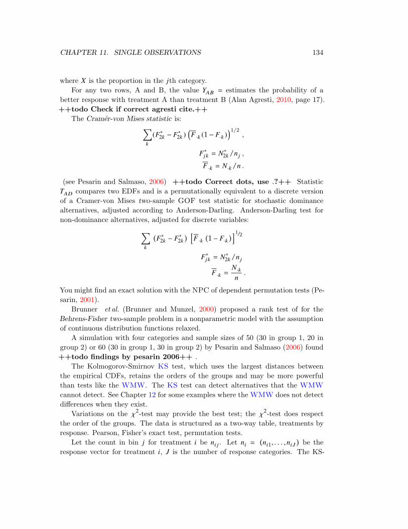
CHAPTER 11. SINGLE OBSERVATIONS 134
where X is the proportion in the jth category.
For any two rows, A and B, the value YAB = estimates the probability of a
better response with treatment A than treatment B (Alan Agresti, 2010, page 17).
++todo Check if correct agresti cite.++
The Cramer-von Mises statistic is:∑
k
(F∗2k − F
∗2k )
(
F ·k (1 − F·k ))1/2
,
F∗jk = N
∗2k/n j ,
F ·k = N·k/n .
(see Pesarin and Salmaso, 2006) ++todo Correct dots, use .?++ Statistic
TAD compares two EDFs and is a permutationally equivalent to a discrete version
of a Cramer-von Mises two-sample GOF test statistic for stochastic dominance
alternatives, adjusted according to Anderson-Darling. Anderson-Darling test for
non-dominance alternatives, adjusted for discrete variables:
∑
k
(
F∗2k − F
∗2k
)
[F ·k
(
1 − F·k)
]1/2F∗jk = N
∗2k/n j
F ·k =N·kn
.
You might find an exact solution with the NPC of dependent permutation tests (Pe-
sarin, 2001).
Brunner et al. (Brunner and Munzel, 2000) proposed a rank test of for the
Behrens-Fisher two-sample problem in a nonparametric model with the assumption
of continuous distribution functions relaxed.
A simulation with four categories and sample sizes of 50 (30 in group 1, 20 in
group 2) or 60 (30 in group 1, 30 in group 2) by Pesarin and Salmaso (2006) found
++todo findings by pesarin 2006++ .
The Kolmogorov-Smirnov KS test, which uses the largest distances between
the empirical CDFs, retains the orders of the groups and may be more powerful
than tests like the WMW. The KS test can detect alternatives that the WMW
cannot detect. See Chapter 12 for some examples where the WMW does not detect
differences when they exist.
Variations on the χ2-test may provide the best test; the χ2-test does respect
the order of the groups. The data is structured as a two-way table, treatments by
response. Pearson, Fisher’s exact test, permutation tests.
Let the count in bin j for treatment i be ni j . Let ni =(
ni1, . . . ,niJ)
be the
response vector for treatment i, J is the number of response categories. The KS-

CHAPTER 11. SINGLE OBSERVATIONS 135
test compares the empirical cumulative distribution functions (ECDF). ++todo
Add to glossary, addgloss.++
Read Agresti’s review on ordered categorical variables (Liu and A. Agresti, 2005),
and on Bayesian methods Hitchcock and Alan Agresti (2005).
The Kruskal-Wallis test is a special case of the proportional odds model. You
can use the proportional odds model to model multiple factors, adjust for covariates,
etc.. See Peterson (1989), Peter McCullagh (1980), and Whitehead (1993).

12 Case Study
After researchers collect a set of observations (data), before any analysis begins, a
measurement scale is applied to the data. The four standard scales are nominal,
ordinal, interval, ratio.
scale A scale is a function that assigns a real number to each element in a set of
observations (for nominal type could tokens work, e.g., Y/N, M/F?)
The ordinal scale assigns a rank to each observation Huberty (1993, see).
The language used is often confusing, we do not have nominal data but data
that has been assigned a nominal measurement scale; we cannot describe the data
with a scale type. Similarly, a variable is not nominal. Often, for a data set,
the measurement scale is not arbitrary, e.g., the amount bid in an auction is best
with a ratio scale. ++todo Check ratio scale.++ Other times the proper
measurement scale is not automatic. For example, the comparison of gas mileage
between three categories (8-, 6-, or 4-cylinder) could treat these categories as interval
or ratio, Hand and Keynes (1993) and Paul F. Velleman and Wilkinson (1993, see).
The chosen measurement scale may depend on the research question; the hypothesis
does not depend on the measurement scale.
For instance in the case described below, if you are interested in difference in
average contribution, then a continuous scale would be necessary, if you are inter-
ested in the effect of treatments on the distribution of contributions, then an ordinal
categorical measurement might work best.
Different types of variables:
nominal Its values are members of an unordered set.
136

CHAPTER 12. CASE STUDY 137
ordinal Its values are members of a discrete ordered set.
continuous Its values are real numbers, time, distance. Sometimes a distinction
is made between interval and ratio, but the distinction is not very useful.
Agresti (see Alan Agresti, 2010) calls a variable with an ordered categorical
scale—ordinal. For ordinal scales, unlike interval scales, there is a clear ordering of
the levels, but absolute distances among them are unknown. An ordinal variable is
quantitative in the sense that each level on its scale is greater or smaller than another
level. For categorical data most statistical methods treat the response variables as
nominal—the results are invariant to permutations of the categories.
Most important whether data are qualitative (nominal) or quantitative (ordinal
or interval).
When choosing a measurement scale the statistics available for that scale should
be considered. If the researcher decides that an ordinal scale will be used, then
a linear model (generally more powerful than X !!->TODO->)<-<- cannot be
applied to the data as it could be if it where assigned a ratio scale.
Ordinal methods can be used with quantitative data, when the response variable
is interval scale rather than ordered categorical. For example, when the response
outcome is a count but count models such as the Poisson do not apply, each obser-
vation can be treated as a single multinomial trial with a finite (hopefully small)
number of ordered categories.
In experimental economics data observed in dictator type games can be assigned
either discrete ordinal, interval, ration. ++todo Check interval.++ In a stan-
dard dictator experiment one half of the subjects are asked to choose a contribution
between zero and a fixed amount. For example, may be able to choose a dollar
amount in { 0,1, . . . ,8 }, which provides for nine discrete categories.
12.1 Comparing Two Distributions
Several statistics (metrics) are available to measure the difference between two em-
phirical cumulative distribution functions ECDF. For example, the absolute value
of the area between them; or their intergrated mean square difference, the maximum
value of the absolute difference between them, this is the Kolmogorov-Smirnov dis-
tance D.
Two tests that are often used by experimental economists (see citet bort) to test
for treatment differences in dictator-type games are the Wilcox-Mann-Whitney and
the Kolmorgorov-Smirnov . The null hypothesis is F = G, where F and G are two
ECDFs; anothe null hypothesis tests the equality of the medians of the ECDFs.
Unfortunately, the process is flawed as I discuss below.
Consider the observations from an experiment with 4 treatments The data in Ta-

CHAPTER 12. CASE STUDY 138
Table 12.1. Distribution of contributions per treatment. .
Treatment 0 1 2 3 4 5 6 7 8 N mean histogram
A 8 3 0 4 0 1 1 1 4 22 3.0
B 8 1 0 2 1 0 3 2 5 22 3.8
C 2 2 1 1 0 2 3 3 8 22 5.4
D 2 1 1 0 1 0 6 1 8 22 5.8
Total 86
ble 12.1 shows the number of subjects who contributed the column amount for each
treatment and contribution category (cell). A common analysis of dictator-type
Table 12.2. P-values for the two-sided paired hypothesis of the dictator treatmens from Ta-
ble 12.1 .
Treatment
Pairs
Asymptotic Exact
WMW KS WMW KS Pearson
A, D 0.01 0.01 0.01 0.00 0.04
A, C 0.02 0.05 0.01 0.03 0.17
B, D 0.07 0.25 0.07 0.15 0.29
B, C 0.10 0.40 0.09 0.29 0.33
A, B 0.55 0.88 0.55 0.51 0.65
C, D 0.82 0.99 0.82 0.92 0.62
games applies the WMW, the KSKolmorgorov-Smirnov and the Pearson-χ2-tests.
The hypothesis’ tests the difference between medians, the equality of the distribu-
tions, and sometimes both.
The two-sided p-values for each pair and the WMW and KS tests (both asymp-
totic and exact) are shown in Table 12.2. The p-values of the two tests are different;
The WMW test provides evidence for a difference between the first four pairs, (the
hypothesis of the original analysis) and the KS provides evidence for a difference
between the first two pairs. The Pearson-χ2-test provides evidence for difference in
only one pair.
In Chapter 7 I argue against the use of multiple methodologies (analysis, tests)
and you can see that each test provides different results; a clear answer to the
initial hypothesis is difficult. The (WMW is not in glossary) test is not valid for
the discrete data of the dictator game and the (KS is not in glossary) test has to
be adapted for discrete data.
The Pearson-χ2-test ignores the ordering of the observations and it loses some

CHAPTER 12. CASE STUDY 139
information and hence efficiency; its p-values are all larger than the KS and WMW
making it a more conservative test. ++todo Is more conservative correct?++
Both the WMW and KS use the ordering of the data; the WMW because it uses the
ranks of the observations. The kS is also a rank test, but it is not very obvious; a
simple example will show that the KS-statistic is different when the order is changed.
In Table 12.3 the first distribution of observations F1 and G1 has a KS statistic of
Table 12.3. KS ordering.
Changing the order of the data changes the KS statistic
f1 g1 F1 G1 ∆1 f2 g2 F2 G2 ∆2
1 0 1 0 1 1 2 1 2 -1
1 0 2 0 2 1 0 2 2 0
1 2 3 2 1 1 2 3 4 -1
1 2 4 4 0 1 0 4 4 0
2 (maximum of |∆1|); when we switch rows 1 and 4 the maximum of |∆1| is 1. So
when the order of the observations is changed the KS statistic can be different. The
χ2-statistic,
∑
i (Observeredi −Expectedi )2
Expectedi,
does not depend on the order of the observations.
Let Y be an ordinal response variable, c the number of categories, n the number
of observations partitioned into the c categories. Let n1,n2, . . . ,nc denote the number
of observations in each category, with n =∑
j n j , and pj = n j/n denote the sample
proportions. We are following the notation of Alan Agresti (2010).
For a randomly selected observation, let π j denote the probability of response
in category j. The cumulative probabilities are
Fj = Pr(Y ≤ j) = π1 + · · · + π j , j = 1,2, . . . ,c.
The cumulative probabilities reflect the ordering of the categories by
0 < F1 < F2 < . . . < Fc = 1.
What summary measures can we apply to ordinal data? One measure is the
median, the minimum j such that Fj ≥ 0.50. For the comparison of groups or treat-
ments this measure can be misleading with discrete ordinal (categorical response):
Changing a single observation can move the median from one category to another,
no matter how many observations you have, this can give a single observation greater
influence on the summary measure than other observations. Two groups can have

CHAPTER 12. CASE STUDY 140
Table 12.4. The median is not the message.
Treatement 0 . . . 5 . . . 10 N Mean Median Histogram
A 5 0 6 0 0 11 2.8 5
B 0 0 6 0 5 11 7.4 5
the same median but the distribution of one group can be shifted relative to the
other group (see Table 12.4 for an example) is another problem.
This may seem to contradict the widespread use of the median, but recall that
the advantage of using the median as measure of central location is its insensitivity
to outliers; in this environment outliers are not a problem. When the observations
have quantitative values, the ordinal scale can be treated as an interval scale, and
the mean of the observations can be used. If there is no obvious quantitative scale,
ordered scores can be assigned to the categories. Two common scores are ridits and
midranks. We will not discuss them here.
The typical research question asks if the treatment effects differ, if so, which
pairs?
Dictator game researchers often use the Kolmogorov-Smirinov, Wilcoxon-Mann-
Whitney, and the Kruskal-Wallis statistical tests. Unfortunately, none of these tests,
as normally used, are appropriate for the type of observations generated by dictator
games. The acWMW tests the equality of the mean of the ranks in an observation
group or treatment, so that it does not always capture differences in the observed
data distribution. To see this, look at the simple example presented in Table 12.5.
Table 12.5. The WMW test example.
Treatement 0 . . . 5 . . . 10 N Mean Sum ranks Histogram
A 2 0 0 0 2 4 5 18
B 0 0 4 0 0 4 5 18
As displayed in Table 12.5 the sum of the ranks for each treatment is 18; since the
number of observations for each treatment is the same the (WMW is not in glossary)
test statistic is zero. No level of significance would reject the null hypothesis of
no treatment effect. But simple observervation shows that the observations from
the different treatments have very different distributions. This is not an extreme
example, treatments A and B presented in Table 12.1 have similar data distributions
as treatment A in Table 12.5.
An understanding of the assumptions of (WMW is not in glossary) test is
required to understand the its proper usage. The (WMW is not in glossary) does

CHAPTER 12. CASE STUDY 141
not always indicate differences in data distributions in the general case, and although
it is often stated as such it only tests for differences in the median under certain
assumptions (they are not always satisfied). So even though the WMW (and other
tests) do not assume that the data are from a parametized probability distribution,
there are still assumptions that must be satisfied.
12.2 WMW assumptions
12.3 Kruskal-Wallis
The discussion on WMW can be easily extended to the Kruskal-Wallis test.
12.4 Kolmogorov-Smirnov
The kolmogorov-Smirnov test, tests the difference between two empiracal distribu-
tions by measuring the maximum difference between the two distributions. Finding
the probability distribution of the max is a difficult problem, so it was necessary to
assume that the data are measured by a continuous scale and that there are no ties.

13 Multivariate
Observations
A multivariate test is based on several variables simultaneously. For multivariate
normal data Hotelling’s T2statistic is the multivariate version of the t-test. The test
requires a large sample to provide a close to exact significance level ++todo how
close++ . An exact significance level can be obtained regardless of the underlying
distribution by use the permutation distribution of Hotelling’s T2. ++todo
What is the in reference to: pg 176 (freedman) page 177 (efron).++
The procedure, algorithm is in(P. I. Good and James W. Hardin, 2009, page 77).
++todo add algorithm++ This or randomizationTest.
See also the section on MANOVA.
Robust Hotelling’s Tsq
A test robust to outliers (including R code) is given by roelant2008 it uses robust
estimation of scale and scatter.
13.1 MANOVA
13.2 Multivariate Ordered Categorical Data
Testing of hypothesis for multivariate ordered categorical variables is known to be
a difficult problem (see Pesarin and Salmaso, 2006) especially when testing for
stochastic dominance. Likelihood ratio tests are particularly difficult.
An extension to multivariate version of the two-sample design with stochastic
dominance alternatives, also called component-wise stochastic dominance. T⋆2MD
142

CHAPTER 13. MULTIVARIATE OBSERVATIONS 143
corresponds to Hotelling’s T2 statistic for two-sample testing for multivariate cat-
egorical variables. ++todo There is another section on multivar ord
cat.++
14 Dependent Observations
Many statistical methods are not applicable when the observations are not indepen-
dent. Serial correlation can invalidate most parametric and nonparametric methods
for computing probability statements such as a confidence interval and p-values.
Examples of dependent observations are
Repeated measures Repeated measures on a single experimental unit. One op-
tion is to treat the series of observations on a single unit as a single multivariate
observation; ++todo Check Good cite section.++ Good (P. I. Good,
2006, section 5.6), Pesarin (Pesarin, 2001, chapter 11) provide permutation
tests. Standard modeling approaches are mixed-effects models or GEE.
Clusters Data gathered from a group who may share experiences, education, val-
ues, or other group characteristics. If stratification is not appropriate: treat
each cluster as a single observation and use a summary statistic as in §11.1
and Mosteller and J. W. Tukey (1977). ++todo Look at these.++
Cluster statistics are unlikely to be identically distributed, variances of the
statistics may depend upon the size of each cluster, hence, a permutation test
based on the statistic is not exact. If the data has many clusters P. I. Good
and James W. Hardin (P. I. Good and James W. Hardin, 2009, page 81) rec-
ommends using the bootstrap, where the samples are drawn on the clusters
rather than the individual observations.
Question is, why is bootstrap OK and the permutation test is not. See sect
on bootstrap §9.8. ++todo Describe why bootstrap OK not permu-
tation.++
144

CHAPTER 14. DEPENDENT OBSERVATIONS 145
Pairwise dependence When data have the covariance is the same for each pair
of observations. The permutation test ++todo For clusters, correct.++
is exact if the observations are normally distributed and almost exact oth-
erwise Erich L Lehmann and J. P. Romano (2005). ++todo Check on
this.++
Group randomized trials See P. I. Good and James W. Hardin (P. I. Good and
James W. Hardin, 2009, page 82) taken from Feng et al. (Braun and Feng,
2001). ++todo Check on Feng cite.++
Moving average or autoregressive process For discussion see Brockwell and
Davis (Brockwell and R. A. Davis, 1987).
Alonso, Litiere, Mohlenberghs (Alonso, Litiere, and Molenberghs, 2008) evaluate
misspecifying the random-effect distribution on inferential procedures.
Hardin and Hilbe (J. W. Hardin and Hilbe, 2003, page 28) specify the correlation
for population-averaged Generalized Estimation Equationss (GEEs) models.
Heidelberger and Welch (Heidelberger and P. D. Welch, 1981) discuss the con-
struction of a confidence interval when data are serially correlated.

15 Repeated Observations
Repeated measures is one form of dependent observations. Other forms are clus-
tering , pairwise dependence, and group-randomized trials. Repeated measures are
sequential observations on a single experimental unit (e.g., subject, group within a
session, session).
We can analyze repeated measures by aggregating the time series of an experi-
mental unit into a single multivariate observation, by repeated-measures ANOVA,
by a mixed-effects model or GEEs.
Probability statements directly asymptotically bootstrapping or by using ran-
domization or permutation tests (see Pesarin, 2001; Pesarin, 2010, Chapter 11) P. I.
Good (and 2010, Section 5.6).
15.1 Power Repeated measures
15.2 Aggregate Single Observation
Aggregate repeated observations to a single statistic. ++todo Aggregate
Hand++ One simple method of repeated observations is to combine the
observations into a single statistic. While it simplifies the problem, there is loss of
information.
146

16 Traditional MANOVA
and ANOVA
16.1 Unstructured Multivariate Approach
MANOVA
The unstructured multivariate approach (normal-theory) applies MANOVA and
Hotelling’s T2statistic,
X =(
X1,Y X2, . . . ,XP
)
(16.1.1)
=
(
Y1, . . . ,)
, (16.1.2)
where
P = number of periods . (16.1.3)
Each observation is a vector of observations for each period (trial). The test requires
the sample size to be greater than the number of periods to estimate a (P × P)
covariance matrix. Hotelling T2 statistic is
T2= ( y − µo )
TS−1p ( y − µo )n, (16.1.4)
n − p
p(n − 1)T2
∼ F . (16.1.5)
Hotelling’s T2 statistic requires that all multivariate observations be independent of
one another, that all observations are metric, and that the covariance matrix be the
same for all observations. It is applicable only to shift alternatives { F[x] = G[x− δ] },and that there is a sufficient number of observations to estimate the covariance
matrix, that is, n > p.
147

CHAPTER 16. TRADITIONAL MANOVA AND ANOVA 148
Based on power considerations, if the data have a distribution close to that of the
multivariate normal and the samples are large, the Hotelling T2 is the appropriate
statistic in the one-sample and two-sample cases.
The stated significance level cannot be relied on for small samples if the data
are not normally distributed (cite Davis, 1982; Srivastava and Awan, 1982).
Hotelling’s T2 is designed to test the null hypothesis of difference between the
distributions of two groups (for example, treated and untreated) against alternatives
that involve a shift of the k-dimensional center of the multivariate distribution. It
is not particularly sensitive to alternatives that entail a shift in just one of the
dependent variables. Boyett and Shuster (1977) provide a more powerful test, the
maximum t-test.
Friedman and Rafesky (J. H. Friedman and Rafesky, 1979) provide a multi-
variate generalization of the distribution-free, two-sample tests of Wald-Wolfowitz
and Smirnov, used for testing FX = FY against the highly nonspecific alternative
FX , FY . It is a generalization of a non-parametric runs test with the ordering
based on a minimal spanning tree.
To detect a simultaneous shift in the means of several variables, use Hotelling’s
T2; to detect a shift in any of several variables, use the maximum t; and to detect
an arbitrary change in a distribution use either Perasin’s method of nonparametric
combination or Friedman and Rafesky’s multivariate runs test.
Tests proposed by vanPutten.1987 and Henze (1988) offer advantages over
Friedman-Rafesky.
16.2 Univariate ANOVA
Univariate ANOVA treats time as a fixed factor.
yi j = µ+ αk + πi + τj + εi j
where
αk is the treatment,
πi is the random session effect,
τj is the fixed factor time, and
εi j is the error.
Σ = (σ2π + σ
2ε )
*..,
1 ρ
· · ·ρ 1
+//-,
where
ρ = σ2π/(σ
2π + σ
2ε ) = Corr(yi j , yi j′) .

CHAPTER 16. TRADITIONAL MANOVA AND ANOVA 149
If Corr(yi j , yi j′) is constant, then this is called sphericity, or circularity. That is,
the correlation between any pair of repeated observations is the same. This is not
a common condition in experimental economics.
Compound Symmetry
If the covariance matrix
Σ p =σ2a11
T+ σ
2 I (16.2.1)
where
Corr(yi j , yi j′) = σ2a (16.2.2)
Corr(yi j , yi′ j ) =σ2 (16.2.3)
Corr(yi j , yi j ) =0 . (16.2.4)
If compound symmetry holds, then the F-ANOVA statistic is more powerful test
than the Hotelling T2. If compound symmetry does not hold, then the ANOVA
F-test is anti-conservative (i.e., rejection decisions cannot be trusted).
If compound symmetry holds the F-ANOVA statistic is more powerful than
Hotelling’s T2; if compound symmetry does not hold then the F-test ANOVA is
anti-conservative , that is, rejection decisions cannot be trusted. In general the
ANOVA F-test holds if the sphericity condition holds.
The usual F-test is distributed as F(t−1), (t−1)(n−1), We can bound the critical
value by F1, (n−1), but F is very conservative, it will accept too often (i.e., not reject
enough). We can use the different bounds on the F-test to construct a classic
methodology:
1. Conduct usual F-test, if fail to reject H0, Stop. The Hypothesis is not signifi-
cant.
2. Conduct test using F1, (n−1), if reject H0, Stop. The Hypothesis is significant.
3. Estimate ε use the Huynh-Feldt test (1976). Use
Fε (t−1),ε (t−1)(n−1)
1
t − 1≤ ε ≤ 1 .
See Sage page 26, anova v. manova. ++todo Do Huynh-Feldt++

17 Mixed-Effects models
Most EE are repeated measures experiments. N subjects are observed on each of k
successive occasions, which possibly correspond to different experimental conditions,
the ith subject yielding the observation yi j on the jth occasion, yi j may be a vector.
Graphic Place Holder
p | a / no mixed effect | \
| x a price/quantity | \ \
| b x a positive slope | \ \
| b x | \
| b
| With mixed effect each subgroup/cohort
q has a negative price/quantity slope.
They are usually replicated, a replication An experiment with n observations per
cell is to be distinguished from having n replications with one observation per cell.
The total is the same but the relevant sources of variation differ. Inferences from
replications have a broader scope than inferences from non-replicated experiments
++todo HOW++ .
EE are nested in the sense that each (subject %IN% group) appears under only
one treatment. We cannot evaluate interaction of subject or group with treatment.
Effects restricted to a single level of a factor are said to be nested within that factor.
150

CHAPTER 17. MIXED-EFFECTS MODELS 151
17.1 Regression
Treat time as a fixed factor, we construct
y = X β + ε, ε ∼ N (0, Σ pi).
or
yi j = µ+ αk + πi + τj + εi j
where
µ = mean
αk = treatment effect
πi = (random/fixed) subject effect
τj = time fixed factor
εi j = error
Yit = Y +Tt + ei , (17.1.1)
where i = unit observed, t = treatment, with treatment t constant across units
(elements). The treatment-effect or stimulus-response relation may depend on the
unit or subject.
Yit = Y +Tit + ei , or Yit = Y +Tt + eit ,
In (17.1.1) there is a common distribution across t for errors. The following equation
Yt = Y +Tt + e
disregards interactions between treatments and units and the variations among units.
We see this in (17.1.1).
Diggle et al. Diggle et al. (2002, page 20) has an analysis of efficiency. The conse-
quences of ignoring correlation when it exists are incorrect inferences and estimates
are less precise than possible.
17.2 Random-Effects Models
Also called two-stage (or multi-stage models),
yi = Zibi + Xiβ + εi ,

CHAPTER 17. MIXED-EFFECTS MODELS 152
where
εi is the within-individual variation (stage 1), and
bi is the between-individual variation (stage 2)
follows from N. M. Laird and Ware (1982). Sketch an outline of the hierarchical
approach using a two-stage model. The first stage specifies the mean and covariance
structure for a given individual. (at the intra-individual level)
E (yi | βi ) = f i (βi ), and Cov(yi | βi ) = Ri .
E [yi | βi ] = f i (βi ), and Cov(yi | βi ) = Ri .
f characterizes the systematic dependence of the response on the repeated measure-
ment conditions for the ith individual (Xi ), Ri is a covariance matrix summarizing
the pattern of random variability associated with the data for the ith individual.
The second stage characterizes the inter-individual variation, consists of a model
for variation in the regression parameters βi , or random variation among individuals.
βi = Ai β + bi Ai = individual-specific information.
bi = error corresponds to the random component of inter-individual variation,
bi ∼ (0,D).
A model formulation and computational methods are described in Lindstrom
and Bates (M. J. Lindstrom and D. M. Bates, 1990), The variance-covariance
parameterizations are described in Pinheiro and Bates (Pinheiro and Douglas M.
Bates, 2000). The different correlation structures available for the correlation argu-
ment are described in Box, Jenkins, and Reinsel (G. E. P. Box, Jenkins, and R. G.
C., 1994), Littel, Milliken, Stroup, and Wolfinger (Littell et al., 1996), Venables and
Ripley (2002). The use of variance functions for linear and nonlinear mixed-effects
models is presented in detail in Davidian and Giltinan (1995).
17.3 Linear Mixed Effects
LME models
1. provide flexibility in modeling the within-group correlation,
2. allow balanced and unbalanced data in a unified framework,
3. flexibility to include multi-levels or nesting, and
4. efficient procedures exist for fitting mixed-effects models.

CHAPTER 17. MIXED-EFFECTS MODELS 153
Also called analysis of grouped data, longitudinal data, repeated measures, blocked
designs, multilevel data, panel data (used in econometrics). Differences in approach
and interpretation depending on discipline.
The basic model is (Charles E. McCulloch, S. R. Searle, and Neuhaus, 2008,
Chapter 6, page 156)
E[yi j
]= µ+ ai + βiεi j
where
µ = overall mean
ai = fixed effects
βi = random effects, and
εi j = error .
A (LME is not in glossary) model consists off two sets of effects plus a constant
and error term. Fixed effects are used for modeling the mean of y. Random effects
govern the variance-covariance structure of y. The main reason for random effects
is to simplify the task of specifying the N (N + 1)/2 distinct elements of Var yN×1.
In a clinical trial experiment a longitudinal design is used for
1. to increase sensitivity by making within subject comparisons,
2. to study changes (time measured in years, months, and days),
3. to use subjects efficiently
.
The design goals 1 or 2 are usually not design criteria in experimental economics.
The time frame for an EE is less than 2 hours, so the subjects them selves are
likely to change. However, EE designs consider measurements before and after an
intervention, such as, the announcement of relevant information. A crossover design
could be also used taking care of hysteresis. The most important reason may be
subject learning of both the rules of the experiment and the actions and reactions
of the other subjects.
For now we will assume that the random effects and errors are Gaussian and
the response variable is continuous. This does not include generalized linear mixed-
effects models Chapter 22.13. See also Diggle et al. (Diggle et al., 2002) .
Model factor as fixed or random effects
Fixed effects Make inferences about particular levels of a factor. Associated with
an entire population or with certain repeatable levels of experimental factors.

CHAPTER 17. MIXED-EFFECTS MODELS 154
Random effects Make inferences about population from which the levels are drawn.
Associated with individual experimental units drawn at random from a popu-
lation. Usually, levels correspond to different subjects or experimental units.
Mixed-effects models have both. See S. S. Searle, Casella, and C. E. McCulloch (S. S.
Searle, Casella, and C. E. McCulloch, 1992) and Vonesh and Chinchilli (Vonesh
and Chinchilli, 1997) who provide a comprehensive overview. Common features :
• Repeated response measurements taken on a number of different units (indi-
viduals).
• Dependence (linear or nonlinear) of the response y on a set of unknown pa-
rameters, β, for each unit.
• Response profiles are similarly shaped across individuals, but may have differ-
ent values of the parameter vector β for different units
• A non-homogeneous pattern of within-individual variability. Possible devi-
ations include serial correlation, and a dependence of variability on mean
response.
• Inter-individual variability between parameters that may be considered ran-
dom, to be related to individual-specific characteristics.
17.4 Basic Model
See Pinheiro and Douglas M. Bates (Pinheiro and Douglas M. Bates, 2000, page
58). Single Level grouping based on N. M. Laird and Ware (1982).
For m experimental units (or group), let ni be the size (which could be one) of
each unit i = { 1, . . . ,m }, and let yi be a ni-dimensional be response vector for the
ith experimental unit. m is the number of experimental sessions or groups (a group
could contain a single person).
yi = Xiβ + Zibi + εi , i = 1, . . . ,m (17.4.1)
where bi ∼ N (0,Ψ), and εi ∼ N (0,σ2I) is a ti × 1 vector of within-session errors.
• Xi is a ti × b design matrix (or known fixed effects) for session i.
• β is a b× 1 vector of regression coefficients (for fixed effects),
• bi is a g × 1 vector of random effects for session i,
• Zi is a ti × g design matrix (or known random effects) for session i (regressor
matrices what is?), The columns of Zi are usually a subset of Xi , and

CHAPTER 17. MIXED-EFFECTS MODELS 155
• ti is the number of periods in session i.
bi , b, εi, and εi′ are independent for all i and i′.
Ψ is a (q × q) symmetric and positive semi-definite matrix. Note the indefinite
model can always be re-expressed as a lower dimensional positive-definite model. bi
has a mean of 0, any non-zero mean for a term in a random-effects model must be
expressed as part of the fixed-effects terms. For computation we define:
Ψ−1
1
σ2
= ∆T∆
since Ψ is positive definite ∆ exists but need not be unique. ++Find ref refer-
ence?++ .
17.5 Estimation
There are a number of methods to compute the MLE. ML estimates of the variance
components σ2εand σ
2b tend to underestimate. An alternative is REML (). See
Patterson and Thompson Patterson and Thompson (1971) Harville (Harville, 1977)
.
The Bayesian framework corresponds to assuming a locally uniform prior for the
fixed-effects β and integrates them out of the likelihood.
ML is invariant to one-to-one transformations of the fixed effects, REML is not
invariant so likelihood ratio tests are not valid for testing fixed effects because there
is a term that changes with a change in fixed effects. The essential difference of the
estimates is σ2=
∑
()2/n with ML and σ2
=
∑
()2/(n − p) with REML.
Optimization of likelihood see Mary J. Lindstrom and Douglas M. Bates (1988), Long-
ford (1993), N. M. Laird and Ware (1982), ++todo Is there a 1983 Laird Ware
or is it 82?++ Dempster, N. Laird, and D. Rubin (1977), ++todo 1979 or
1977++ Pinheiro and Douglas M. Bates (2000) for LME.
EM ++todo EM is?++ iterations and Newton-Raphson iterations, also
Quasi-Newton (Thisted). EM quickly brings parameters into range but converges
slowly. Newton-Raphson is more computationally intensive, can be unstable far
from optimum but close to optimum converges quickly. Hybrid approach is to use
EM the Newton-Raphson.
For inference on parameters, the approximate distribution of MLE and REML
estimates derives from asymptotic results. Pinheiro (1994) finds that under certain
regularity conditions the MLE of LME and REML estimates are consistent and
asymptotically normal.
The general method for fitting nested models is the LRT Erich L Lehmann and
J. P. Romano (2005). It can be used when REML and both models have the same

CHAPTER 17. MIXED-EFFECTS MODELS 156
fixed-effects specification. A statistical model is nested within another if it is a
special case of the other model. For example, let
y = α + β1x1+β2x2 + ε
Some nested models are:
y = α + 3x1 +β2x2 + ε
y = α +β2x2 + ε
A non-nested model is:
y = α + bz +β2x2 + ε
If you use REML to estimate the parameters, then you can only test if the fixed
effects are the same.
To make comparisons the AIC, (Akaike, 1974) and Sakamoto et al. (Sakamoto,
Ishiguro, and Kitagawa, 1986), and the BIC, Schwarz (Schwarz, 1978), are usually
used.
AIC = −2 ℓ(θ | y) + 2n
BIC = −2 ℓ(θ | y) + 2n log(n)
where n = the number of parameters.
Use the ++todo From P and B page 84++ LRT to evaluate the significance
of terms of the random-effects structure. Stram and Lee (1994) argue this is a
conservative test; i.e., the for χ2k2−k1
is greater than it should be. The more
restricted model has parameters set on boundary, e.g., 0. Possible to simulate
++todo what?++ .
17.6 Assessing Models
A long used measure for assessing a linear model is the R2. R
2 is the sum of squares
due to the fitted model divided by the total sum of squares. It is usually not used
to assess model fit for comparison since it does not penalize for the number of
parameters in a model.
R2 cannot determine if there are too many parameters in a model, the addition
of noise (a variable) will increase the R2. Criteria like Akaike Information Criterion
(AIC) and Bayesian Information Criterion (BIC) penalize the likelihood function for
the number of parameters in a model. ++todo Is it only nested models.++
Minimum Description Length (MDL), a totally different approach that over-
comes the limitations of AIC and BIC. There are several measures stemming from
MDL, like normalized maximum likelihood or the Fisher Information approximation.

CHAPTER 17. MIXED-EFFECTS MODELS 157
The problem with MDL is that its mathematically demanding and/or computation-
ally intensive.
Parametric Bootstrap, which is quite easy to implement.
When stipulating normally distributed errors (and other assumptions)
AIC = −2 ln(likelihood) + 2k, and
BIC = −2 ln(likelihood) + ln(N )k ,
where
k = model degrees of freedom, and
N = number of observations .
Both are based on a maximum likelihood estimate penalized by the number of free
parameters to try to avoid over fitting.
The“best”model in the comparison group minimizesAIC orBIC.BIC penalizes
more than AIC when N is more than 7, so its application will produce simpler
models.
An informative and accessible derivation of AIC and BIC by Brian Ripley can
be found here presentation, (ripley.derivation ).
AIC, there exist many adjustments (AICc) to account for certain conditions
which make the original approximation bad. This is also present for BIC. More
exact (but still efficient) methods exist, such as Fully Laplace Approximations to
mixtures of Zellner’s g-priors (BIC is an approximation to the Laplace approxima-
tion method for integrals).
It seems that there is no consensus on which is better or what to use; and there
is not much of a basis to make a comparison
17.7 Hypothesis Tests for Fixed-effects Terms
To make hypothesis tests on the fixed-effects terms the LRT can be defined for ML
fits of a model only (not for REML fits). However, it is not recommended, the LRT
tends to be anti-conservative and sometimes very much so, Littell et al. (see 1996,
section 1.5).
Another approach (Pinheiro and Douglas M. Bates, 2000, pg 89–90) is to con-
dition on the estimates of the random-effect variance-covariance parameters, using
conditional tests. In Splus and R summary (result.lme) fixed effects.
The overall effect of a factor should be assessed with an ANOVA table not by
examining the p-values of the associated fixed-effect parameters. Splus/R ANOVA
(result.lme).

CHAPTER 17. MIXED-EFFECTS MODELS 158
17.8 Multiple levels
A multiple level model (e.g., two nested levels of random effects) can be constructed
as ++todo As what++ .
Let yi j be the response vector, i = 1, . . . ,m, j = 1, . . . ,mi . m is the number
of first level groups (sessions), mi is the number of second-level groups within the
first-level groups (subjects), mi j is a vector of X. ++todo Fix this.++
yi j = Xi jβ + Zi, jbi + Zi jbi j + εi j
where
bi ∼ N (0, Ψ1),
bi j ∼ N (0, Ψ2),
εi j ∼ N (0, σ2 I),
and where
Xi j is a ni j × p matrix,
Zi, j is a ni × q1 matrix,
Zi j is a ni × q2 matrix,
bi is a q1 dimensional vector, and
bi j is a q2 dimensional vector.
bi , bi j , and εij are independent for all i.
Some of the literature calls this model a three-level model, because it has three
levels of random variation. The experimental design literature calls this a two-level
model because it has two levels of nested levels.
17.9 Heterogeneity
The basic model is flexible but restricts within-group errors to be independent and
identically distributed with E [ε] = 0, and Var(ε) = σ2. The within group errors
can be specified as heteroscedastic (unequal variance) or correlated or both.
yi = Xiβ + Zibi + εi i = 1, . . . ,m
bi ∼ N (0,Ψ)
εi ∼ N (0, σ2Λi )
where Λi is a positive definite matrix parameterized by a small fixed set of param-
eters λ, and bi and εi are independent for all i.
Charles E. McCulloch, S. R. Searle, and Neuhaus (Charles E. McCulloch, S. R.
Searle, and Neuhaus, 2008, page 177) prefer ML and REML to (ANOVA is not

CHAPTER 17. MIXED-EFFECTS MODELS 159
in glossary) as does S. S. Searle, Casella, and C. E. McCulloch (1992). They give
the following reasons:
Maximum Likelihood (ML) and (REML is not in glossary) are based on the
well-respected maximum likelihood principle; but if any solutions are negative you
have to make an adjustment (Charles E. McCulloch, S. R. Searle, and Neuhaus,
2008, page 37–40,Sect. 2.2.b).
ML provides an estimate of fixed effects, REML does not ++todo Check if
true++ . REML for balanced data solutions (not estimators) ++todo check
what++ are (ANOVA is not in glossary) and despite their ability to be negative
are minimal variance unbiased under normality, and minimal variance quadratic
otherwise. There is no guarantee for unbalanced data.
Restricted Maximum Likelihood (REML) uses the degrees of freedom for fixed-
effects model, this is important when the rank of X is large in relation to sample
size. ++todo Large - meaning what?++ Because β is not involved in REML,
the estimate of variance components are invariant to β.
REML is not as sensitive to outliers as ML (vebyla1993 ).
Hastie and Robert Tibshirani (2000).
17.10 Bootstrapping Mixed-Effects Linear Model
In any bootstrapping procedure sampling must maintain a model structure.
To bootstrap in a mixed-effects linear model you would do sampling with re-
placement in a way that maintains a model structure.
So your data is divided into groups and you do not want to mix the data from
one group into the data from another.
Temp psuedo code display
For i = 1 to number of samples
--->For j = 1 to number of groups Ng
------>group j has mj observations
------>sample (Sj) with replacement from the group of observations
--->End For j
---> (S1, \ldots, SNg) is the bootstrap sample
--->Fit a model with bootstrap sample

CHAPTER 17. MIXED-EFFECTS MODELS 160
--->Collect estimates bi and errors ei
End For j
With collected estimates can construct bootstrap confidence intervals.
The simplest is Efron’s percentile method which takes the 2.5 percentile and the
97.5 percentile from these ordered bootstrap estimate to be the endpoint of a 95
percent confidence interval.
Efron and Tibshirani’s B. Efron and R. Tibshirani (1993)
Efron and Tibshirani B. Efron and R. Tibshirani (1986)
17.11 Bayesian Mixed-Effects Models
Maximum a posteriori estimation.

18 Data Presentation
At their best, graphics are
instruments for reasoning.
Tufte (2012)
As researchers we want other researchers to read our research. One way to make
research accessable is to ensure that it is readable. The visual presentation of your
statistical information might decide whether someone understands what you are
trying to say. In the next few sections I present a few ideas for data presentation.
18.1 You have the data, now what?
• Data collection and processing.
• Computation of test statistics.
• Interpretation of results.
• Presentation of results; graphical and tabular; not in statistical jargon; the
statistical tests in the appendix.
• Graphical illustrations should be simple and pleasing to the eye and avoid
purely decorative features—good graphical displays use most of the ink to
convey important information P. I. Good and James W. Hardin (see 2009,
page 149).
161

CHAPTER 18. DATA PRESENTATION 162
Graphic pointers:
• Do not connect discrete points, they may be misinterpreted as a continuous
data values.
• Do not use more dimensions in the display than the data has.
• No pie charts.
• The graphic and caption should include all salient information; in isolation
the graphics message should be apparent to another person.
Examples of good and bad graphics reside at bad graphics. Also, J. W. Hardin
and Hilbe (J. W. Hardin and Hilbe, 2003, pages 143–167) describes graphics for
assessing model accuracy.
18.2 Making Visual Displays
18.3 Principles for Effective Visual Display of Data
ACCENT
The essence of a graph is the clear communication of quantitative information. The
ACCENT principles emphasize, or accent, six aspects which determine the effective-
ness of a visual display for portraying data. ++todo Set up definition list++
Web page of good and bad graphic examples: graphic examples
Apprehension: Ability to correctly perceive relations among variables. Does the
graph maximize apprehension of the relations among variables?
Clarity: Ability to visually distinguish all the elements of a graph. Are the most
important elements or relations visually most prominent?
Consistency: Ability to interpret a graph based on similarity to previous graphs.
Are the elements, symbol shapes and colors consistent with their use in previ-
ous graphs?
Efficiency: Ability to portray a possibly complex relation in as simple a way as
possible. Are the elements of the graph economically used? Is the graph easy
to interpret?
Necessity: The need for the graph, and the graphical elements. Is the graph a
more useful way to represent the data than alternatives (e.g., table, text)?
Are all the graph elements necessary to convey the relations?

CHAPTER 18. DATA PRESENTATION 163
Truthfulness: Ability to determine the true value represented by any graphical
element by its magnitude relative to the implicit or explicit scale. Are the
graph elements accurately positioned and scaled?
“Blind Lemon Jefferson, the great blues musician, was once asked why there
were so few white blues-men. He replied, Knowin’ all the words in the dictio-
nary ain’t goonna help if you got nuttin’ to say.”
Adapted from Burn (1993). ++todo Is there a better set of criteria,
Wilkinson, 2005 grammar of graphics, Tukey++
See Van Belle, 2002, aberrant values are more apparent in graphics, and Chance
22:1, winter 2009, pg 51; Friendly and Kwan (2009) for collinearity biplots, Sarkar
lattice vis; cleveland visual 1993; Cleveland’s Elements (Cleveland, 1994).
Graphics for visualizing a single set of data:
• One-way strip chart, symbol at each data point darker/thicker if more than
datum at a point.
• Box plot: 0, 25, 50, 74, 100% quartiles, interquartile range (IQR) = box
around 25th to the 75th percentile of the distribution.
• Combination box and strip chart.
• Box and whiskers plot (see recent Am Stat).
Box Plots
++todo Check if the word should be box plots or box-plots?++
Box plots were invented by Tukey for EDA. Showing nonparametric statistics,
box plots have proven to be quite a good exploratory tool, especially when several
box plots are placed side by side for comparison. The most striking visual feature
is the box which shows the limits of the middle half of the data (the line inside the
box represents the median). Extreme points are also highlighted. Box plots show
not only the location and spread of the distribution of the data but also indicate
the skewness or asymmetry of the distribution. A box-plot summarizes a great deal
of information very clearly; it is good at showing up errors—efficiency should not
be greater than 100% or negative.
A box plot displays the center half of the data (the box) with the median marked.
The top and bottom of the box are defined by the hinges (see below). By default,
whiskers are drawn to the nearest value not beyond a standard span from the hinges.
Points beyond the end of the whiskers (outliers) are drawn individually.
Splus/R note. Specifying range = 0 forces the whiskers to span the full data
range. Any positive value of range multiplies the standard span by range.

CHAPTER 18. DATA PRESENTATION 164
The standard span is 1.5 × (upper hinge − lower hinge). See Frigge, David C.
Hoaglin, and Iglewicz (1989) for implementations of the boxplot. Dumbgen and
Riedwyl (2007) On Fences and Asymmetry in Box-and-Whiskers Plots.
Graphic Place Holder
Put a box plot image example
As original defined by Tukey a box plot uses hinges for the lower and upper
limits of the box. The hinges are the median value of each half of the data where
the overall median defines the halves. Hinges are similar to quartiles. The main
difference between the two is that the depth (distance from the lower and upper
limits of the data) of the hinges is calculated from the depth of the median. Hinges
often lie slightly closer to the median than do the quartiles. The difference between
hinges and quartiles is usually quite small.
Graphic Place Holder
Show difference in hinges and quantile for boxplot
++todo Show difference in hinges and quantile for boxplot++
Many statistical packages and elementary statistics books replace the hinges
with the first quartile (q1) and the third quartile (q3). The distance from q3 to q1
is called the inter-quartile range. The whiskers (lines with crosses on them) extend
to the furthest points still within 1.5 inter-quartile ranges of q1 and q3. Beyond the
whiskers, all outliers are shown. Often the outliers up to a specified distance (e.g.,
3 inter-quartile ranges beyond q1 and q3) are displayed by a different symbol than
the outliers beyond the specified distance.
18.4 Box and Whiskers Plot
Box-and-whiskers plots display five-point summaries and potential outliers in graph-
ical form.
To constuct a boxplot:
1. Determine the 5-point summary for the data.
2. Draw on graph paper a box extending from Q1 to Q3.
3. Inside the box, draw a line that locates the median.

CHAPTER 18. DATA PRESENTATION 165
4. Calculate the interquartile range (IQR = Q3 − Q1)
5. Calculate fences 1.5 hinge-spreads below and above the hinges:
a) The lower fence FenceLower = Q1 − 1.5 IQR.
b) The upper fence FenceUpper = Q3 − 1.5 IQR.
c) Do not plot these fences.
6. Any value above the upper fence is an upper outside value. Any values below
the lower fence is a lower outside value. Plot these values separate points on
the graph.
7. The largest value still inside the upper fence is called the upper inside value.
The smallest value still inside the lower fence is the lower inside value. Drawn
whiskers from the upper extent of the box (upper hinge) to the upper inside
value, maximum, and from the lower extent of the box bottom hinge to the
minimum.
Graphic Place Holder
Show a box and whisker plot. See
wp2/stats/boxWhiskerExampleComplex.pdf
18.5 Interpretation of boxplots
Boxplots show less detail than stemplots, but still provide insight into the central
location, spread, and shape of a distribution.
When you look at a boxplot, consider the following elements:
Central location: The line in the box locates the median. In addition, the box
locates the middle 50 percent of the data.
Spread: The length of the box is called the hinge-spread. This corresponds to
++todo what++ . The IQR is a good quantifier of a distribution’s spread. In
addition, The whiskers from tip-to-tip (the whisker-spread) quantifies its spread.
The maximum and minimum are visible as well.
Shape: Shape is difficult to judge except when the sample is large, in which case
symmetry or lack of symmetry will be visible.
See D. C. Hoaglin, Mosteller, and J. W. Tukey (1983), R. McGill, J. W. Tukey,
and Larsen (1978), John W. Tukey (1990), and P. F. Velleman and D. C. Hoaglin
(1981).

CHAPTER 18. DATA PRESENTATION 166
Histograms
References
Sachs (Sachs, 1984, pages 53–54) provides a method for calculating the number of
classes k ≃ 1+ 3.32 log n, and a constant class width b ≈ √xmax − xmin . Other avail-
able methods for calculating the number of classes are Sturges, Freedman-Diaconis,
and Scott.
See Venables and Ripley (2002), and Denby and Mallows (2009),
Pie Charts
Pie charts are common in business and popular economics, but rare in academic
publishing or scientific research. They are generally not recommended and the
same data can be displayed in a bar chart. If pie charts are used it is recommended
to use them only when the sum of all categories is meaningful, for example, for
percentages of a whole.
Visual research shows that comparison by angle is less accurate than comparison
by length ++todo by AT&T Bell Laboratories when++ . Compare pie
chart and bar chart for the same data. Most subjects have difficulty ordering the
slices in the pie chart by size; when the bar chart is used the comparison is much
easier (Cleveland, 1994, pages 86–87).
It is easier to compare length than to compare area to see a difference among
categories.
Wilkinson (Wilkinson, 2005, page 23) critizes the pie chart, Tufte (tufte2001 )
++todo check which tufte book++ says do not use, as does van Belle (Van
Belle, 2008, pages 160–162).
Remark 18-1
The earliest known pie chart is credited to William Playfair’s Statisti-
cal Breviary of 1801 Playfair, 2005. Florence Nightingale (1820–1910)
published a polar area diagram in “Diagram of the causes of mortality
in the army in the East” in Notes on Matters Affecting the Health, Ef-
ficiency, and Hospital Administration of the British Army and sent to
Queen Victoria in 1858. �
18.6 Making Tables
18.7 Making Tables and Growing Cucumbers

CHAPTER 18. DATA PRESENTATION 167
The graphical method has considerable superiority for the exposition of
statistical facts over the tabular. A heavy bank of figures is grievously
wearisome to the eye, and the popular mind is as incapable of drawing
any useful lessons from it as of extracting sunbeams from cucumbers.
(A. B. Farquhar and H. Farquhar (1891, pg. 55))
Despite the admonishment from Farquhar and Farquhar, tables are the format
choice of many researchers (see Feinberg and Howard Wainer, 2011). Three rea-
sons why this might be so are
• data is usually stored in a table, either in a text file or and EXCEL type data
sheet,
• Tables are easy to prepare, and
• data extraction is easy from tables.
A table uses icons (numbers) to convey information and one way to make tables
more comprehensible is to use space, the judicious placement of the data in the xy
plane of the table (just as is done in a graph.) There are three constructs ++todo
is constructs correct word++ to improving the table:
• rounding,
• emphasize summary statistics, and
• meaningful ordering of rows and columns.
Rounding
++todo check article Yucel, He, and Zaslavsky (2008)++ .
We have all seen (and if you are like me constructed) tables with numbers
written to four digits or more. I do not know what I was thinking, but I and most
people cannot comprehend more than two or three digits easily; usually, do not care
about accuracy of more than three digits; and usually cannot justify more than three
digits of accuracy statistically, Cleveland and Robert McGill (Cleveland and Robert
McGill, 1984) performed psychophysical experiments to confirm this. More digits
in a list of numbers make it harder to compare them. For example, in Table 18.1
lists made up revenues (in dollars) for five companies, it also lists the revenues in
billions of dollars. A natural spoken statement of revenue for firm A is 256 billion
dollars; we would usually not recite the 12 digits of the revenue in dollars. I see the
entries in the column labelled Billions of dollars easier to compare.
Sometimes the argument against rounding is that we are compromising accuracy.
Numbers should not be presented with any more accuracy than is statistically or

CHAPTER 18. DATA PRESENTATION 168
Table 18.1. Example of Rounding.
Percent
Corporation Revenue ($) Billions ($) error
A 256,328,236,345 256 0.1
B 232,893,222,185 233 0.3
C 186,125,234,483 186 0.1
D 122,834,293,784 123 0.7
E 119,382,398,812 119 0.3
computationally justified. To explain statistical accuracy, suppose the mean of a
set of auction prices is 10.7263 with a standard deviation of σ. For fourth digit
accuracy the standard error would have to be less than 0.00005. The sample size
(n, the number of observations) that can justify this level of accuracy is:
standard error = 0.00005 = σ/√
n (18.7.1)√
n /σ = 1/0.00005 = 20,000 (18.7.2)
n = (20,000)2= σ400 million. (18.7.3)
So a large sample size is necessary for fourth digit accuracy. Increasing the sample
size increases the level of accuracy of the calculated mean.
For a guide to the appropriate number of digits see Ehrenberg (Ehrenberg, 1977)
and van Bell (Van Belle, 2008, table 7.4).
Emphasize important data
When constructing a table it is often important to provide summary statistics, usu-
ally the last row or column, to make it easier to emphasize differences in between
columns or rows. Making the summary statistics bold and spaced further apart
from the other columns or rows, will draw the eye to them.
Ordering
Suppose we have performed several auction experiments grouped by four treatments.
And we now want to present the data, one row for each session. In what order do
we list the sessions? If our emphasis is on efficiency in the table we should list
the experiments so that the lowest (or highest) efficiency is presented first with the
rest subsequently ordered by efficiency. If we are most interested in revenue, then
the sessions should be ordered by revenue. This gives the reader an easy way to
compare sessions (or treatments); the lowest and highest efficiency is obvious, and
any sessions with similar efficiencies are clumped together.

CHAPTER 18. DATA PRESENTATION 169
The Table
Once we have determined what goes into our table we have to format the table.
Here are some rules that are in common usage:
1. Never, ever use vertical lines1
2. Never use double lines.
3. Put the units in the column heading (not in the body of the table).
4. Always precede a decimal point by a digit; thus 0.1 not just .1.
5. Decimal points should line up in a column.
6. Do not use ‘ditto’ signs or any other such convention to repeat a previous
value. In many circumstances a blank will serve just as well. If it does not,
then repeat the value.
7. Put heavy lines at the bottom and top; heavier than the mid rules (middle
lines).
Dyke (1997)
The following is based on Koschat (2005). A substantial bibliography of aca-
demic research articles, a dedicated major research journal2, and several books3
attest to the importance of statistical graphics as an area of research.
Tables are indeed widely used, and in many statistical reports and research
papers more space is devoted to tables than graphs. Yet this obvious prominence is
barely reflected in the broader statistical discourse. Tables as displays of information
are rarely a topic in statistical education, are rarely a point of discussion in statistical
practice and, within the field of statistics, do not appear to receive much, if any,
attention from researchers.
An early contribution on the design of statistical tables to the statistical litera-
ture is Walker and Durost’s text (Walker and Durost, 1936). Since, most articles
on this topic have been published mostly by a small handful of researchers, notably
Ehrenberg Ehrenberg, 1981; Ehrenberg, 1986 Wainer (H. Wainer, 1992; H. Wainer,
1997a; H. Wainer, 1998; H. Wainer, 1993) and Tufte (Tufte, 2003). The latter two
authors acknowledge tables as a valuable format for communicating information in
their books Tufte (Tufte, 1990; Tufte, 1997; Tufte, 1983; H. Wainer, 1997b), but in
1A line is called a rule by typographers. ++todo Check in package booktabs; if by
typographers.++2The Journal of Graphical and Computational Statistics3John W. Tukey, 1977; Mosteller and J. W. Tukey, 1977 and Chambers et al., 1983 and Cleve-
land, 1994

CHAPTER 18. DATA PRESENTATION 170
the statistical community these texts are mostly referred to for their consideration
of statistical graphics. Outside statistics, books on document design occasionally
have sections on the construction of tables (Bigwood, Spore, and Seely, 2003; Harris,
2000; Shriver, 1997).
The prescription for the design of a table is straightforward. Arrange numbers—
and it is usually numbers— in parallel rows and perpendicular columns. A table is
a simple structure for arranging numbers. These two defining attributes— the well-
known structure and the use of numbers—provide the major rationale for using
tables. There is an implied commonality to all the numbers in the same row, and
to all the numbers in the same column. This common understanding of a table’s
structure is a good reason to use tables. There are other good reasons for using
tables, for example:
• A numerical display often presents data in their original form.
• Data presented in numerical form can be easily manipulated and transformed,
a graphical display might need interpolation to recover a number.
• Numbers in a table usually need less of an explanation than the elements of a
graphical display.
For the table to be an effective display of data, its entries must be easy to
compare; entries and comparisons that are of special interest should be prominently
displayed and easy to find.
Choice of Columns and Rows
A first step in the construction of a table requires a decision on which entries to
arrange in rows and which entries to arrange in columns. In general, numerical
comparisons are easier made within columns than within rows, this is supported by
research by Hartly (Hartly, 1981; Hartly, 1985).
Arrangement of Rows and Columns
Of equal importance are the relative arrangement of rows and the relative arrange-
ment of columns. Rows whose entries one wishes to compare should ideally be
displayed close together, and the same holds true for the arrangement of columns.
Often the data themselves suggest such a grouping. For example, it may be use-
ful and informative to arrange rows such that the entries in the principal column
of interest appear sorted. Because we tend to read from left to right and top to
bottom, a table’s left upper quadrant is likely to receive most of a reader’s initial
attention. Hence one should consider arranging rows and columns such that the
entries of greatest interest fall into the left upper quadrant.

CHAPTER 18. DATA PRESENTATION 171
Presentation of Numbers
It is usually not possible to arrange all entries that one should, or might want to,
compare in adjacent and vertically aligned positions. In such instances the reader
has to commit, however briefly, at least one of the numbers to be compared to
memory. The number of distinct digits that most people retain easily after a single
pass is more or less limited to seven (G. A. Miller, 1956). It is therefore good
practice to transform the data such that five digits or fewer represent each table
entry, if possible. Often this can be accomplished by adjusting the scale and, by
rounding, limiting the number of digits retained. Thus, rounding is an important
step with an additional benefit. Usually the left-most digits of a number are more
important than the digits to the right. Retaining too many digits hinders the reader
from paying attention to the more important digits.
Simple Graphical Elements
A table entry is characterized not only by its numerical value but by its position
within the table. The effectiveness of a table presentation depends in part on how
easy it is to determine an entry’s position within the table and to connect it to its
row and column labels.
Two simple graphical elements, lining and shading help as the redesigned table
in Table ?? illustrates. Shading changes the background color for selected rows
and columns, creating groups that are easier to compare. Lining refers to the judi-
cious and parsimonious addition of lines to the basic rectangular data display. The
emphasis is on judicious and parsimonious because, as in Figure ??, the problem
is often not that there are too few but that there are too many lines. Separating
each pair of adjacent rows and columns by a line results in a useless grid that does
nothing to help the reader orient herself. On the other hand, the horizontal lines
added to the table in Figure ?? define horizontal bands of five rows each, with
two complementary benefits. On the one hand, the bands are sufficiently wide and
distinct to be easily traceable as the reader’s glance moves from left to right
There are other typographical elements one can consider with benefits perhaps
similar to or complementary to lining and shading. Adherents of the minimal use of
ink school of thought might argue that in Figure ?? an effect similar to lining could
have been achieved simply by increasing the line spacing every five rows. Arguably,
an effect similar to shading could have been achieved by, instead of shading selected
cells, choosing a font distinct in type, style, or size for the entries in these cells.
Figure 6 includes an example of such alternatives.
The tabulation made explicit in Figure ?? is an essential step in the construction
of a histogram. This frequency tabulation, when first proposed more than 300 years
ago by John Graunt (see, Tapia and Thompson 1978), was duly acknowledged as an
important and original scientific accomplishment. In a standard histogram this step

CHAPTER 18. DATA PRESENTATION 172
is implicit with the result that, in my experience, most readers— even those who
have received statistical training in the form of an introductory statistics course—
have difficulties interpreting them. On the other hand, few people have difficulties
interpreting the table in Figure 5 and subsequently interpreting the accompanying
bar chart.
Tables that present statistical results can be graphically enhanced.
Some other references in comments.
R coding tables
The apsrtable R package which offers an alternative display of Tables, compared to
xtable, and reporttools described in the JSS,
Temp R code display
library(Hmisc)
x=rnorm(1000)
y=rnorm(1000)
lm1=lm(y~x)
slm1=summary(lm1)
latex(slm1)
or given a dataset dta,
latex(summary(dta)).
R Coding test file output
Temp R code display
use print
print(summary(~x + y), prmsd=TRUE, digits=1)
capture or write to text file:
capture.output(print(summary(~x + y), prmsd=TRUE, digits=1),
file="out.txt")
use sink:
sink(file=output.txt, type="output");
print(summary(~x + y), prmsd=TRUE, digits=1),
sink(),

CHAPTER 18. DATA PRESENTATION 173
18.8 What to Report
The assignment of experimental units to treatments and how they were randomized;
the assignment of subjects to experimental units; were they randomized individually
(experimental unit is the subject) to treatments or were treatments randomized to
groups of subjects (the experimental unit is the group).
1. Power and sample size calculations (prior).
2. Describe the assignment of subjects to treatments.
3. Detail exceptions and missing data.
4. Measures of dispersion and central tendency if applicable. Median, arithmetic
mean, geometric mean; standard deviation, standard error, or bootstrap con-
fidence interval.
5. Provide confidence intervals instead of p-values.
6. Any sources of bias.
7. Describe practical significance.
8. Formal statistical inference for predetermined hypothesis.
See Lang and Secic (Lang and Secic, 1997, page 177) for reporting or meta-
analysis.
Tufte (tufte ) for tables versus graph.
Parkhurst (Parkhurst, 1998) for arithmetic vs geometric mean.
When reporting p-values derived from nonrandom samples, it is best to provide
(and internalize) a disclaimer such
as “While, strictly speaking, inferential statistics are only applicable in the
context of random sampling, we follow convention in reporting significance lev-
els as convenient yardsticks even for nonrandom samples.” (Michael Oake) See
Michael Oakes’s Statistical inference: A commentary for the social and behavioral
sciences (Oake, 1986).
When reporting the mean, it is better to report the standard deviation rather
than the variance. The standard deviation is expressed in the same units as the
mean and it is easier to construct confidence intervals.

Part II
Two
174

19 Individual Behavior
Studying individual behavior can be the either a primary or secondary purpose for
analysis.
For example see El-Gamal and Grether avoid the data snooping.
175

20 Single-Case Designs
See Single-Case and Small-N Experimental Designs: A Practical Guide to Random-
ization Tests Todman (2001).
The usual inferential statistics are frequently invalid for use with data from
single-case experimental designs.
Randomization (Exact) tests can provide valid statistical analyses for all de-
signs that incorporate a random procedure for assigning treatments to subjects or
observation periods, including single-case designs.
176

21 Testing Single Sample
Designs
21.1 Single-sample Testing
The most used type of this design is in theory testing. For example, is the market
price in the double auction the competitive equilibrium price? In this setting we
do not have randomization over treatments for causal inference of treatment effect;
there is no treatment effect.
The standard approach is to test the hypothesis H0 average price = competitor price,
and then to use a t-test or a nonparametric test. This begs the question, what is
the probability model used used for inference?
Suppose we have the results of three double auction sessions A, B, and C; each
with a series of observed prices.
Temp R code display
Give data series.
Plot a series of double auction prices
Find mean and variance of observed prices for each session
and overall.
Is the price close to the competitive equilibrium, does it converge? With mean
and variance v is 1.1. What does a variance of 1.1 say, is that small, large? How
are we to decide?
177

CHAPTER 21. TESTING SINGLE SAMPLE DESIGNS 178
If we construct a confidence interval around p-mean, we get pminus and pplus;
does the competitive equilibrium fall in the range? Problem, we cannot construct a
confidence interval because we have no probability model ++todo Check freed-
man for term.++ we have what Freedman call’s a get set. There is no sampling
distribution, no randomization to form probabilities.
One approach is to treat the data with EDA; we can give the data statistics
and make visual plots— in most experiments looking at the price series and we
can determine closeness or convergence. Statistical hypothesis testing, confidence
intervals have no inferential strength ++todo What is this.++
How strong is our conclusion, is it just an anomaly. Are the three sessions alike
or dissimilar.
If we want a statistical basis for our conclusions, we have to make specific our
question. What is the more specific question (hypothesis).
If we observe p that has t = p− pce distance from the ce; what is the probability
that we observe p close to pc.
Ho : p , pce, Ha : p = pce.
Probability of small, first we have to decide what is small and how to find the
probability of t.
We can treat the possible actions of the participants as our sample/observation
space.
Construct a one-sample randomization test
Ha
What is the probability that we observe the allocation efficient outcome if each
trade/nontrade is equally likely.
Say we have demand schedule p,q 10,4 8,3 6,2 4,1 and a supply schedule p,q 4,
1 6,2 8,3 10,4.
Derived from two buyers resale values (two), and two sellers costs (two). Let If
each buyer and seller are randomly matched we find the following distribution: F.

22 Possible Additions
22.1 Incomplete
The following sections are incomplete and are intended as suggestions for additional
chapters in either part I or II.
22.2 Meta-analysis
Meta-analysis is, in essence, a collection of techniques to synthesize the results of
a literature, often in conflict, and look at it as a coherent whole. See good.errors
page 110 provides guidance. See Lang and Secic 1997, reporting or meta-analysis
page 177 ff.
22.3 Brain Imaging
Fmri; Functional images JGCS 18:1, mar 2009, pg 216. anals applied stats, 2008
2:1 Stat Sci, 2008, 23:4, 439.
22.4 Text Analysis
22.5 Path Models
Reference (see D. A. Freedman, 2009, Chapter 6)
179

CHAPTER 22. POSSIBLE ADDITIONS 180
22.6 Factor Analysis
Godino, Batanero, Jaimex 2001 and good.erros page 209. For principal compo-
nent analysis, see JCgraph stats, 18:1, 2009, p 201; Adaptive shrinkage; Dimension
reduction, stat sci, 2008, 23:4 pg 485–501.
Factor analysis is a.
Principal component analysis is a technique to decompose an array of numeri-
cal data into a set of orthogonal vectors (uncorrelated linear combinations of the
variables) called principal components.
22.7 Effect Size
Measures of effect size in ANOVA are measures of the degree of association between
and effect (e.g., a main effect, an interaction, or a linear contrast) and the dependent
variable. It is the correlation between an effect and the dependent variable. The
square is the proportion of variance in the dependent variable that is attributable
to each effect.
Four commonly used measures of effect size in ANOVA are
• eta squared, η2,
• partial eta squared, η2p ,
• omega squared, ω2, and
• intraclass correlation, ρI .
η2 and η2
p are estimates of the degree of association in the data. ω2 (fixed effect
models) and the intraclass correlation ρI (random effect models) are estimates of
the degree of association in the population. η2 is computed as
η2= SSeffect/SStotal .
One of the problems with η2 ++todo Is this correct++ its value is depen-
dent the other effects. For that reason many people prefer an alternative computa-
tional procedure called the η2p . Some authors e.g., Tabachnick and Fidell (Tabach-
nick and Fidell, 1989) call η2p an alternative computation of η2. η2
p is computed
as
η2p =
SSeffect
(SSeffect + SSerror)
it is the proportion of the effect and error variance that is attributable to the effect.
η2p differs from η2 in that the denominator includes the SSeffect plus the SSerror rather
than the SStotal.

CHAPTER 22. POSSIBLE ADDITIONS 181
The sums of the η2p values are not additive. They do not sum to the amount
of dependent variable variance accounted for by the independent variables. It is
possible for the sums of the η2p values to be greater than 1.00. In general, η2
describes the amount of variance accounted for in the sample. An estimate of the
amount of variance accounted for in the population is ω2. Because η2 and η2p are
sample estimates and ω2 is a population estimate, ω2 is always going to be smaller
than either η2 or η2p .
From Murphy and Myors (1998) and Kirk (1982). The strength of association
between independent variable Y and dependent variables X , if both X , Y are numer-
ical can be computed by the linear correlation
r =
√
SSXY/SStotal .
++todo XY correct?++ When the independent variable is qualitative esti-
mates of strength of association between X and Y for a population. ρI (intraclass
correlation) and ω2 both indicate the proportion of variance in X accounted for
by specifying the Y treatment level classification. ρI applies to the random-effect
model ω2 applies to a fixed-effect model.
They are identical in general meaning (hayes1963 ) (referenced by Kirk 1982 Kirk
(1982))
ρI =(MSBG − MSWG)
(MSBG + (n − 1)MSWG)
see Haggard (Haggard, 1958) .
ω2=
(
SSBG − (k − 1)MSWG
)
(
SStotal + MSWG
)
WG = Within groups, BG = Between groups. MS Within groups is also called
MSerror. MS Between groups is also called MStreatment. The notation of Winer et al.
and others.
A significant F ratio for treatment effects indicates that there is an association
between X and Y . ω2 and ρI are measures that indicate the strength of the associa-
tion. An alternative method of interpreting the importance of sources of variation is
in terms of variance components. “An F ratio only provides information concerning
the probability that effects are or are not equal to zero, it does not tell us whether
effects are large or small.” ( (Kirk, 1982, page 127) ).
Variance components:
σ2β is an estimate of σ2
β (the variance of the means of the treatment populations).
σ2β =
(
MSB − MSresidual)
n
Trivial effects can achieve statistical significance if the sample is sufficiently large (Kirk,
1982, page 135).

CHAPTER 22. POSSIBLE ADDITIONS 182
22.8 Completely randomized factorial designs
ω2XA=
(
(SSA − (p − 1)MSw.cell))
(
(SStotal + MSw.cell))
ω2XB=
(
(SB − (q − 1)MSw.cell))
(
(SStotal + MSw.cell))
ω2XAB
=
(
(SSAB − (p − 1)(q − 1)MSw.cell))
(
(SStotal + MSw.cell))
If the value of ω is negative, then set it to zero. If the F-statistic is significant
then the value of ω will be positive (Kirk, 1982, page 198). ++todo proof of
this++
ρ(I)XA=
σ2B
σ2A + σ
2B + σ
2AB + σ
2ε
Estimating the magnitude of experimental effects and statistical power (Winer,
1971, page 405). For completely randomized factorial designs with equal sample
sizes.
ωA2effect =
variance estimate for effect of interest
total variance estimate
The basis for constructing such estimates is the expected values of the mean squares dodd.schultz.1973
One index (of several possible) is:
ω2effect =
SSeffect − (dfeffect)MSerror
SStotal + MSerror
ω2α =
θ2α
θ2α + θ
2β + θ
2α β + σ
2ε
For a 2 × 2 design with factors A and B
p = number of levels of factor A
q = number of levels of factor B
n = number of observations in each cell
xi jk = observation k in cell i j

CHAPTER 22. POSSIBLE ADDITIONS 183
ABi j =
∑
k
xi jkn Ai =
∑
j
ABi jq
B j =
∑
i
ABi j p G =∑
i
Aip =∑
j
B jq
αi = Ai −G β j = B j −G
θ2α =
∑
i α2i
pσ
2α =
∑
i α2i
p − 1
εi jk = xi jk − ABi j
s2i j =
∑
k
εi jk (n − 1)
MSerror =∑
i
∑
j
∑
k
ε2i jk pq(n − 1)
MSa = nq∑
i
(Ai −G)2(p − 1)
MSab =n∑
i
∑
j (ABi j − Ai − B j +G)2
(p − 1)(q − 1)
Confidence Interval for Effect Size
The effect size is an estimate so we can calculate the confidence interval.
Cohen’s d is
d = *,
n1 + n2
n1n2
+
d2
2(n1 + n2 − 2)+-(
n1 + n2
n1 + n2 − 2
)
(22.8.1)
the variance of Cohen’s d is
*,
n1 + n2
n1n2
+
d2
2(n1 + n2 − 2)+-(
n1 + n2
n1 + n2 − 2
)
, (22.8.2)
where n1 and n2 are the sample sizes of the two groups being compared and d is
Cohen’s d. Taking the square-root of this variance gives the standard error of d.
22.9 Legal Evidence
See Good and Freedman.
22.10 Hints and Tools
A few hints to experimenters, when you design an experiment:

CHAPTER 22. POSSIBLE ADDITIONS 184
• Specify important characteristics of the environment. Convince colleagues,
funders, engineers, or others that you do not have to throw in the kitchen sink
or replicate the market exactly.
• Write the instructions first, if you cannot write a simple set of instructions,
then you need to redesign your thinking about the problem.
• Formulate the statistical analysis before you run the experiments. It does you
no good if after the experiments you have data that are difficult to analyze.
Example of bad economic experiment see Mark Walker, Oliver Kim, The free
rider problem: Experimental evidence, public choice, 1984.
22.11 What to Do
When you design an experiment:
1. Write the instructions, if you cannot write a simple set of instructions then
you need to change your approach to the problem.
2. Formulate the statistical analysis. It does you no good if after the experiments
you have data that are difficult to analyze.
3. Specify important characteristics of the environment. Convince colleagues,
funders, and engineers that you do not have to throw in the kitchen sick or
replicate the market exactly.
4. Test software.
5. Test allocation/optimization algorithms.
6. Test instructions/descriptions to participants.
7. Find holes.
22.12 Other Things
Stochastic approximation, monte-carlo, robbins-, jcgs 18:1, march 2009, pg 184.
Review Guidelines
Papers with guidelines for reviewers:
Bacchetti (Bacchetti, 2002) , Finney (Finney, 1997) , Cherry (Cherry, 1998)
,Light and Pillemer (Light and Pillemer, 1984) ,Vaisrub (Vaisrub, 1985) .

CHAPTER 22. POSSIBLE ADDITIONS 185
22.13 General Linear Model
For design Issues of GLM, see Stat Sci 21/3 Aug/06 page 376.
22.14 Overview
The glm is a useful generalization of ordinary least squares regression. It stipulates
that the random part of the experiment (the distribution function) and the system-
atic portion of the experiment (the linear predictor) are related by a function called
the link function.
In a glm, the data (Y ) are assumed to be generated from a distribution function
in the exponential family (a very large range of distributions). The expected value
µ of (Y ) is
E (Y ) = E (Y ) = µ = g−1(Xβ) (22.14.1)
where X is the experiment design matrix, β is a vector of unknown parameters, Xβ
is the linear predictor, and g is the link function.
The random component is a function V of the mean: ++todo Fix this.++
Var(Y ) = Var(µ) = Var (g−1
(Xβ)). (22.14.2)
It makes computations easier if the variance is distributed as an exponential fam-
ily distribution. The unknown parameters β can be estimated with maximum-
likelihood, quasi-maximum-likelihood, or Bayesian techniques.
22.15 Components of the GLM Model
The General Linear Model (GLM) consists of three elements.
• A design matrix X known by the experimenter.
• A distribution function f, (usually) from the exponential family.
• A linear predictor η = Xβ, describing the expected value.
• A link function g such that E (y) = µ = g−1
(η).
The exponential family of distributions contain the probability distributions,
parameterized by θ and τ, whose density functions can be expressed in the form
f y (y ; θ, τ) = exp
(
a(y)b(θ) + c(θ)
h(τ)+ d(y, τ)
)
. (22.15.1)
τ, is called the dispersion parameter.The functions a, b, c, d, and h are known.

CHAPTER 22. POSSIBLE ADDITIONS 186
Link functions
The link function provides the relationship between the linear predictor and the
distribution function (through its mean). There are many commonly used link
functions, and their choice can be somewhat arbitrary. However, it is important to
match the domain of the link function to the range of the distribution function’s
mean.
Table 22.1. Common link functions..
Distribution Name Link Function Mean Function
Normal Identity Xβ = µ µ = Xβ
Exponential Inverse Xβ = µ−1µ = (Xβ)
−1
Gamma Inverse Xβ = µ−1µ =
(
Xβ)−1
Poisson Log Xβ = ln (µ) µ = exp (Xβ)
Binomial Logit Xβ = ln(
µ
1−µ)
µ =exp (Xβ)
1+exp (Xβ)
Multinomial Logit Xβ = ln(
µ
1−µ)
µ =exp (Xβ)
1+exp (Xβ)
22.16 Examples
Linear regression
The simplest example of a glm is linear regression. Here the distribution function is
the normal distribution with constant variance and the link function is the identity.
Binomial data
When the response data Y are binary (taking on only values 0 and 1), a natural
distribution function is the binomial distribution; µi is the probability of Yi taking
on the value one. The usual link function is the logistic function:
g(p) = ln
(
p
1 − p
)
. (22.16.1)
Any inverse CDF cumulative density function (CDF) can be used for the link
since the CDFs range is [0,1], the range of the binomial mean. The normal CDF
Φ is a popular choice and yields the probit model. Its link is
g(p) =Φ−1
(p) .. (22.16.2)
Using the identity link for binomial data can be problematic as the predicted proba-
bilities can be greater than one or less than zero. The variance function for binomial
data is given by:
Var(Yi ) = τµi (1 − µi ) , (22.16.3)

CHAPTER 22. POSSIBLE ADDITIONS 187
where the dispersion parameter τ is usually one. When it is not, a model called the
binomial with over-dispersion or quasi-binomial.
Count data: the Poisson
Count data are modeled by the Poisson distribution; the logarithm is used as the
link function. The variance function is proportional to the mean:
Var(Yi ) = τµi , (22.16.4)
where the dispersion parameter τ is usually one. When it is not, a model is called
the Poisson with over-dispersion or quasi-Poisson.

A R
A.1 What is R?
R is a system for statistical computation and graphics.1 It consists of a language
plus a run-time environment with graphics, a debugger, access to certain system
functions, and the ability to run programs stored in script files. It is free software
distributed under a GNU-style copyleft and is an official part of the GNU project
http://www.gnu.org/. 2
The inspiration for R is the S system from Bell Labs. The earliest begin-
nings of S came from discussions in the spring of 1976, among a group of five
people at Bell Labs: Rick Becker, John Chambers (the principal designer), Doug
Dunn, Paul Tukey and Graham Wilkinson. See http://cm.bell-labs.com/cm/
ms/departments/sia/S/history.html for further information on “Stages in the
Evolution of S”.
A.2 List of Helpful Web Sites
• R Installation and Administration (R-admin): http://cran.r-project.org/
doc/manuals/R-admin.html
• An Introduction to R: http://cran.r-project.org/doc/manuals/R-intro.
html
1Much of the following information is from the R project FAQ and introduction. R has a homepage at http://www.R-project.org/.
2More on the history and a detailed description can be found in the R FAQ and the introductionto R.
188

APPENDIX A. R 189
• The R FAQ: http://cran.r-project.org/doc/manuals/R-FAQ.html
• R Language Definition: http://cran.r-project.org/doc/manuals/R-lang.
html
• R data import and export: http://cran.r-project.org/doc/manuals/
R-data.html, a quide to reading from and writing to various formats, such
as spreadsheets, databases, and network connections.
• CRAN: http://cran.r-project.org/, The “Comprehensive R Archive Net-
work”CRAN is a collection of sites which carry identical material, consisting
of the R distributions, contributed extensions, documentation for R, and R
binaries.
• R-help Mailing List: http://www.r-project.org/mail.html Discussions
about problems and solutions using R.
A.3 Starting R
If the software is installed correctly, then entering the command R at the commandprompt will start an interactive R session. You should see something like the fol-lowing:
R version 2.15.1 (2012-06-22) -- "Roasted Marshmallows"
Copyright (C) 2012 The R Foundation for Statistical Computing
ISBN 3-900051-07-0
Platform: sparc-sun-solaris2.10 (32-bit)
R is free software and comes with ABSOLUTELY NO WARRANTY.
You are welcome to redistribute it under certain conditions.
Type 'license()' or 'licence()' for distribution details.
R is a collaborative project with many contributors.
Type 'contributors()' for more information and
'citation()' on how to cite R or R packages in publications.
Type 'demo()' for some demos, 'help()' for on-line help, or
'help.start()' for an HTML browser interface to help.
Type 'q()' to quit R.
>
The last line with the ‘> ’ is waiting for your input. When you want to exit theinteractive R session enter ‘q()’, you should be asked the question

APPENDIX A. R 190
Save workspace image? [y/n/c]:
Enter ‘y ’ if you want to have your current work available next time you start an R
session, see §A.3 for more details.
Some basics
Here are some basic commands that you need to know:
> # prompt, commands are case sensitive
> q() # quit
+ # continuation prompt
# # comment
x <- 10 # assign 10 to x, x = 10
^c, ^break # interrupt
x <- 1:10 # assign vector 1, 2, \dots, 10 to x
a <- c( b, c ) # combine b and c into a: a <- c( 1/2, (1:3)^2 )
Getting Help
To get help for a command, type: ?command or help(command), for example,to find information about the command anova enter help(anova) or ?anova at thecommand prompt ‘> ’. See ?help for more details. For example,
help(anova) # or ?anova
returns
anova package:stats R Documentation
Anova Tables
Description:
Compute analysis of variance (or deviance) tables for one or more
fitted model objects.
Usage:
anova(object, ...)
Arguments:
object: an object containing the results returned by a model fitting
function (e.g., 'lm' or 'glm').
and so on ..
When you are finished reading the help file, enter a ‘q ’ to return to the R command
line.
Installing Packages

APPENDIX A. R 191
##
## To install the package named "packageName" use the command
> install.packages("packageName")
## For example
> install.packages("knitr")
> install.packages("hmisc")
## It is a good idea to install one package at time
## so you can decipher any problems.
Reading and Writing Text files
The use of encodings, unless you need to write in a language other than english it
is best to keep to basic ASCII. Write to a text file to make things as portable as
possible. Includes things to watch for when exporting (writing) to text files:
• Precision
• Header line
• Separator
• Missing values
• Quoting strings
• Encodings
Input and diverting output to a file
If commands are stored in an external file, say commands.R in the current workingdirectory, then they may be executed in an R session with the command
> source("commands.R")
The function
> sink("output.lst")
given before the source command will divert all subsequent output from the consoleto an external file output.lst. The command
> sink()
restores it to the console. When using the command line, command such as 2+2
prints the output to the console. In a sourced file values are not printed unless you
print it. To print a value use the print command, print(2 + 2). You can also use
source(file, echo=TRUE) to have all output printed.Sometimes the output can be difficult to read, because of scientific notation. To
make the output more readable, set the option scipen.

APPENDIX A. R 192
## do some simple calculations
x <- 3 + 3
print(x)
[1] 6
x <- sqrt(2)
print(x)
[1] 1.414
## Set the option
options(scipen = 5)
## do the same calculations again
x <- 3 + 3
print(x)
[1] 6
x <- sqrt(2)
print(x)
[1] 1.414
Data permanency and removing objects
The entities that R creates and manipulates are known as objects. These may bevariables, arrays of numbers, character strings, functions, or more general structuresbuilt from such components. During an R session, objects are created and storedby name. The R command
> objects()
## or alternatively
> ls()
can be used to display the names of (most of) the objects which are currentlystored within R. The collection of objects currently stored is called the workspace.To remove objects the function rm is available:
> rm(x, y, z, ink, junk, temp, foo, bar)
##
## cleaning up workspace, removing all objects use:
##
> rm(list = ls(all = TRUE)).
All objects created during an R session can be stored permanently in a file for
use in future R sessions. At the end of each R session you are given the opportunity
to save all the currently available objects. If you indicate that you want to do this,

APPENDIX A. R 193
the objects are written to a file called .RData5 in the current directory, and the
command lines used in the session are saved to a file called .Rhistory.
When R is started at later time from the same directory it reloads the workspace
from this file. At the same time the associated commands history is reloaded.
To avoid strange errors and complications, only ‘A-Za-z0-9’ should be used in
variable names and blanks should not be used in directory or filenames.
Commands are separated either by a semi-colon (‘;’), or by a newline. Elemen-
tary commands can be grouped together into one compound expression by braces.
Comments can be put almost anywhere, starting with a hashmark (’#’) everything
to the end of the line is a comment.
Recall past commands
The vertical arrow keys on the keyboard can be used to scroll forward and backward
through a command history, it can then be edited.
Display graphics
Lattice functions such as xyplot() create a graph object, but do not display it
(the same is true of ggplot2 graphics, and Trellis graphics in S-Plus). The print()
method for the graph object produces the actual display. When you use these
functions interactively at the command line, the result is automatically printed,
but in source() or inside your own functions you will need an explicit print()
statement.
Give a graphic example.
% print variables
% print(x)
++todo Give a plot graphic Example.++
Accuracy
The only numbers that can be represented exactly in R’s numeric type are integersand fractions whose denominator is a power of 2. Other numbers have to be roundedto (typically) 53 binary digits accuracy. As a result, two floating point numbers willnot reliably be equal unless they have been computed by the same algorithm, andnot always even then. For example
a <- sqrt(2)
a * a == 2
[1] FALSE
a * a - 2

APPENDIX A. R 194
[1] 4.441e-16
all.equal(a * a, 2)
[1] TRUE
The command all.equal() compares two objects using a numeric tolerance of
Machine double.eps0.5. For more information, see David Goldberg, What Every
Computer Scientist Should Know About Floating-Point Arithmetic (Goldberg, 1991).
To quote from The Elements of Programming Style by Kernighan and Plauger: “10.0
times 0.1 is hardly ever 1.0” (Kernighan and Plauger, 1978).

B Reproducible Research
The R packages Sweave Leisch (2002) and Knitr (Xie, 2013) are tools that allow
embedding R code for complete data analyses in latex documents. The purpose is
to create dynamic reports, which can be updated automatically if data or analysis
change. Instead of inserting a prefabricated graph or table into the report, the
master document contains the R code necessary to obtain it. All data analysis
output (tables, graphs, tests, etc.) is created and inserted into the final latex
document. The report can be automatically updated if data, analysis, or format
change, which allows for truly reproducible research.
195

C LATEX
LATEX (Lamport, 1994) has learning curve but provides man advantages. Besides
the math and text formatting, it provides easy integration of statistical analysis into
a document (a paper, a thesis or a book) with the knitr (Xie, 2013) package. The
is also a package labbook which I have adapted to the economic-labbook package.
++todo Set up economic labbook++ .
196

D Probability Distributions
Probability distributions are the basis of many statistical models. The binomial
distribution is a model of the number of successes (from a binary set of success or
failure) in n repetitions.
The Poisson distribution is a model of counts of the occurrance of an event in a
unit of time.
The exponential and gamma distributions are models of time between events;
for example waiting time or failure times.
The normal distribution is used in many situations, and is also used as an
approximation to other distributions.
Standard Probability Distributions
The uniform distribution:
p(x) =1
b− a, x ∈ (0,1) . (D.0.1)
The exponential distribution:
p(x) = we−wx, x ∈ (0,∞), w > 0 . (D.0.2)
The gamma distribution:
p(x) =c(cx)
w−1e−cx
Γ (w), x ∈ (0,∞), w > 0, (D.0.3)
where
Γ (w) =
∫
I
yw−1e−y dy . (D.0.4)
197

APPENDIX D. PROBABILITY DISTRIBUTIONS 198
The beta distribution:
p(x) =Γ (a + b)
Γ (a)Γ (b)xa−1
(1 − x)b−1, x ∈ (0,1), a > 0, b > 0 . (D.0.5)
If X ∼ Gamma(α,θ) and Y ∼ Gamma(β,θ), and X and Y are independent, then:
X/(X +Y ) ∼ Beta(α, β) .
A simulation in R:
Temp R code display
> m <- 2^16
> x <- rgamma(m,1,1)
> y <- rgamma(m,1,1)
> a <- x/(x+y)
> quantile(a,1:9/10)
The Cauchy distribution :
p(x) =1
π(
1 + x2) , x ∈ (−∞,∞) . (D.0.6)
The log-normal distribution:
p(x) =1
σx√
2πexp { − 1
2(ln x − wσ
)
2
}, x ∈ (0,∞) . (D.0.7)
The normal distribution:
p(x) =
(
σ√2π
)−1
exp { − 1
2
(
x − u
σ
)2
}, x ∈ (−∞,∞) . (D.0.8)
The Laplace distribution:
p(x) =β
2e−β |x |, x ∈ (−∞,∞) . (D.0.9)
The Pareto distribution:
p(x) =β − 1
c
(
c
x
)β
, x ∈ I = (c,∞), c > 0 . (D.0.10)
The Weibull distribution:
p(x) = k xk−1e−x
k
x > 0 . (D.0.11)

APPENDIX D. PROBABILITY DISTRIBUTIONS 199
D.1 Special Distributions
Normal
The distribution has a thin tail, see Appendix Appendix E for some properties of
the normal distribution.
Student T Distribution
As the degrees of freedom increases the Student t-distribution appoaches a normal
distribution ++todo is this true++ .
Cauchy
A Student t-distribution with one degree of freedom is a Cauchy distribution. It is
well known distribution with thick tails.
The Cauchy distribution does not have a mean. A sample from the Cauchy dis-
tribution does have mean. As the sample size increases the mean does not converge
but bounces around (it is erratic), and the sample median behaves well ++todo
whatever that means++ .
The Cauchy distribution does have a median, and the sample median converges
to that median.
The probability distribution of the sample median for a sample of n = 2k + 1
from a Cauchy distribution is
f (x) =n!
(k!)2
(
1
4− 1
π2
arctan2x
)k1
π(1 + x2), for k = 1, . . . . (D.1.1)
The variance is
Var x =2(n!)
(k!)2πn
∫ π/2
0(π − y)
kyk cot2
y dy , (D.1.2)
and is finite for k ≥ 2.1
Remark D-1
When a probability distribution has both a mean and a variance, the
variance of the sample mean is inversely proportional to the number of
samples. This helps the sample mean converge, but does not quarantee
that it will converge. �
++todo continuous or other requirements++
1David (1981, page 50) The book credits rider.1999 P. R. Rider, JASA 55: 322–323.

E Normal Distribution
E.1 Normal Properties
One
If a joint probability density satisfies independence and spericity, then it is a normal
distribution. Define:
Independence For x ∈ ℜ and n > 1, if the joint probability density fn with
marginal probability densities f1 satisfies
fn (x1, x2, . . . , xn ) = f1(x1) f1(x2) · · · f1(xn ) (E.1.1)
, then it is independent.
Spericity If the joint probability density satisfies
fn (x1, x2, . . . , xn ) = gn
(
Σni=1x
2i
)
(E.1.2)
, then it is spherical.
Normal distribution The univariate normal distribution is
f1(xi ) =1√
2π σexp
(
− 1
2σ2x
2i
)
(E.1.3)
Theorem E.1.4 (Herschel-Maxwell) Let Z ∈ ℜn be a random vector for which
• (i) projections into orthogonal subspaces are independent and
200

APPENDIX E. NORMAL DISTRIBUTION 201
• (ii) the distribution of Z depends only on the length ‖Z ‖.
, then Z is normally distributed.
Proof E.1.5 Herschel-Maxwell Spherical symmetry tells you that f1(x) is a func-
tion of x2, i.e.,
f1(x) = g1(x2). (E.1.6)
Independence plus spherical symmetry implies
g1(u)g1(0) = g2(u) and g1(u)g1(v) = g2(u + v) ∝ g1(u + v) (E.1.7)
Therefore, rescaling g1 into h1 so (E.1.7) is an equality, we derive the identity
h1(u)h1(v) = h1(u + v) (E.1.8)
for which the only solution is of the form
h1(u) = exp (αu) , α ∈ ℜ . (E.1.9)
Thus,
f1(x) =1
√
2πσ2exp *
,−x
2
2σ2+- , σ ∈ ℜ
+, (E.1.10)
since only negative factors α lead to densities.
The above from George Cobb (Cobb, 2011, page 54).
++todo Typo: u + 1 instead of u + v++
Two
A standardized Gaussian distribution on ℜ can be defined by its density:
1√2π
e−x2/2 (E.1.11)
Lukacs (Lukacs, 1942) shows that the sampling distributions of the sample mean
and variance are only independent for the normal distribution. Independence of the
sample mean and variance characterizes the normal distribution. Feller (See also
Feller, 1966, page 86) cites R. C. Geary (geary ). ++Find ref R. C. Geary++
If X and Y are i. i.d. with finite variance with X + Y and X − Y independent,
then X and Y are normal. So independence of mean and standard deviation follows
from independence of X +Y and X −Y , but not the other way around.
The continuous distribution with fixed variance which maximizes differential
entropy is the Gaussian distribution.
A. M. Mathai & G. Perderzoli(Mathai and Perderzoli, 1997) prove:

APPENDIX E. NORMAL DISTRIBUTION 202
Theorem E.1.12 Let X1, . . . ,Xn be independent random variables. Then∑n
i=1 ai xiand
∑ni=1 bi xi are independent, where aibi , 0, if and only if Xi are normally dis-
tributed.
There must be a condition such as ∠a,b〉 = 0 missing in the theorem statement
above. For example if n = 2, ai = bi = 1, X1 + X2, and X1 + X2 are not independent.
++todo Check for inner product symbols.++
If A = a1 ⊕ a2 ⊕ · · · ⊕ am, for m ≤ n, where ai are row vectors of dimension nisuch that
∑mi=1 ni = n and ⊕ denotes the direct sum, then the random vector Y has
independent coordinates.
This is not hard to see since Y1 is measurable with respect to σ(X1, . . . ,Xn1), Y2
is measurable with respect to σ(Xn1+1, . . . ,Xn1+n2), etc., and these σ -algebras are
independent since the Xi are independent by definition.
This result still holds if we consider matrices that are column permutations of
the matrix A described above.
For a normal distribution, if AA⊤= D for some diagonal matrix D, then the
coordinates of Y are independent. This is easily checked with the moment-generating
function.
Note: Suppose X1 and X2 are i. i.d. with finite variance. If X1 + X2 is indepen-
dent of X1 − X2, then X1 and X2 are normal distributed random variables.
The result due to Bernstein (Bernstein, 1941). A proof can be found in Feller
or Bryc (2005, chapter 5, page 61). It was generalized by Lukacs and King (1954).
In the case where A cannot be written as a direct sum of row vectors, there is a
distribution for X such that Y does not have independent coordinates.
We have:
Theorem E.1.13 (Lukacs and King (Lukacs and King, 1954)) Let X1,X2, . . . ,Xn
be n independently (but not necessarily identically) distributed random variables with
variances σ2i , and assume that the nth moment of each Xi (i = 1,2, . . . ,n) exists. The
necessary and sufficient conditions for the existence of two statistically independent
linear forms Y1 =∑n
i=1 aiXi and Y2 =∑n
i=1 biXi are:
• Each random variable which has a nonzero coefficient in both forms is nor-
mally distributed, and
•∑n
i=1 aibiσ2i = 0 .
where σ2s is the variance of Xs (s = 1,2, . . . ,n).
Let η and xi be two independent random variables with a common symmetric
distribution such that
Pr
(�����xi + η√
2
����� ≥ t
)
≤ Pr(‖xi ‖ ≥ t) . (E.1.14)

APPENDIX E. NORMAL DISTRIBUTION 203
, then these random variables are Gaussian. This is the Bobkov-Houdre Theo-
rem (Kwapien, Pycia, and Schachermayer, 1996).
Stein’s Lemma provides a very useful characterization. Z is standard Gaussian
if and only if E [ f′(Z )] = E [Z f (Z )] for all absolutely continuous functions f with
E [‖ f′(Z )‖] < ∞.
Cantelli Conjecture
The conjecture by Cantelli dates back from 1917:
Theorem E.1.15 If f is a positive function on ℜ and X and Y N (0,1) indepen-
dent random variables such that X + f (X )Y is normal, then f is a constant almost
everywhere.
If non-continuous functions are allowed, then Victor Kleptsyn and Aline Kurtzmann
have a counter example Cantelli (1918) Kleptsyn and Kurtzmann (2012).
Others
Suppose one is estimating a location parameter using i. i.d. data { x1, . . . , xn }. If x is
the maximum likelihood estimator, then the sampling distribution of x is Gaussian.
A non-degenerate infinitely divisible random variable X has a normal distribu-
tion if it satisfies
− lim supx→∞
log Pr(|X | > x)
x log(x)= ∞ . (E.1.16)
This result characterizes the normal distribution in terms of its tail behavior.
A short proof is: If X is standard normal, then
x Pr(X > x)/ϕ(x) → 1 as x → ∞ ,
so log Pr(X > x) − log ϕ(x) + log x → 0 .
But 2 log ϕ(x) ∼ −x2
and so the result follows.
Computing the Normal
To compute the normal (or error function) Cody (see 1969).

F Proofs
F.1 Proof of KS Distribution Free
The Kolmogorov-Smirnov statistic (over the class of distributions of continuous
random variables) is distribution-free for a finite sample. That is, the distribution
of the test statistic does not depend on the underlying distribution of the data
(under the null hypothesis).
Proof F.1.1 Let F and G be continuous distributions, and Xi ∼ F and Yi ∼ G be
independent i. i.d. sequences of size n. Then
nFn (x) = |{ i : Xi ≤ x }| = |{ i : F (Xi ) ≤ F (x) }| ,and
nGn (x) = |{ i : Yi ≤ x }| = |{ i : G(Yi ) ≤ G(x) }| .
Under the null hypothesis F = G, sup |Fn (x) − Gn (x) | is equal in distribution to the
same statistic obtained from two independent U (0, 1) samples of size n.
Under the null hypothesis, the asymptotic distribution of the two-sample Kolmogorov-
Smirnov statistic is the Kolmogorov distribution, which has CDF
Pr(K ≤ x) =
√2π
x
∞∑
i=1
e−(2i−1)
2π
2/(8x2) .
The p − values can be calculated from this CDF.
204

Glossary
Akaike Information Criterion This is.. 156, 157, 207
ANalysis Of COVAriance This is.. 126, 207
ANalysis Of VAriance This is.. 53, 126–129, 148, 149, 207
Asymptotic Relative Efficiency Compare efficiency of estimators.. 87, 207
Bayesian Information Criterion This is.. 156, 157, 207
Confirmatory Data Analysis This is.. 52, 53, 207
Cumulative Distribution Function A probability function todo.. 64, 76, 120, 186, 207
Empirical Cumulative Distribution Function Given N ordered data points Y1,Y2, . . . ,Yn the
ECDF is defined as EN = n(i)/N , where n(i) is
the number of points less than Yi . This is a step
function that increases by 1/N at the value of each
ordered data point.. 118, 137, 205, 207
Empirical Distribution Function This is.. 112, 118, 207
Experimental Economics The variation of experimental design used in eco-
nomics.. 3, 26, 27, 38, 150, 153, 207
Exploratory Data Analysis This is.. 52, 53, 101, 163, 207
goodness-of-fit This is.. 119, 207
Kolmogorov-Smirnov this 2.. 117–119, 121, 134, 207
Maximum Likelihood This is.. 159, 207
maximum likelihood estimator This is.. 55, 133, 207
205

GLOSSARY 206
power 1 − β. 115
Restricted Maximum Likelihood This is.. 159, 207

Acronyms
AIC Akaike Information Criterion. 156, 157
ANCOVA ANalysis Of COVAriance. 126
ANOVA ANalysis Of VAriance. 53, 126–129, 148, 149
ARE Asymptotic Relative Efficiency. 87
BIC Bayesian Information Criterion. 156, 157
CDA Confirmatory Data Analysis. 52, 53
CDF Cumulative Distribution Function. 64, 76, 120, 186
CE Competitive Equilibrium. 29, 125
ECDF Empirical Cumulative Distribution Function. 118,
137, 205
EDA Exploratory Data Analysis. 52, 53, 101, 163
EDF Empirical Distribution Function. 112, 118
EE Experimental Economics. 3, 26, 27, 38, 150, 153
GEE Generalized Estimation Equations. 145
GLM General Linear Model. 185
GOF goodness-of-fit. 119
KS Kolmogorov-Smirnov. 117–119, 121, 134
ML Maximum Likelihood. 159
MLE maximum likelihood estimator. 55, 133
REML Restricted Maximum Likelihood. 159
207

ACRONYMS 208
RSM Response Surface Methodology. 3
WMW Wilcoxon-Mann-Whitney. 99, 109, 110, 115, 134

Bibliography
Agresti, A. and B. A. Coull (1998). “Approximate is better than ‘exact’ for interval
estimation of binomial proportions.”In: The American Statistician 52.2, pp. 119–
126.
Agresti, A. and B. Finlay (1997). Statistical Methods for the Social Sciences. 3rd ed.
Upper Saddle River, NJ: Prentice Hall.
Agresti, Alan (1990). Categorical Data Analysis. New York, NY, USA: John Wiley
& Sons.
— (2010). Analysis of ordinal categorical data. 2nd ed. Hoboken, NJ: John Wi-
ley&Sons.
Akaike, H. (1974).“A new look at the statistical model identification.”In: Automatic
Control, IEEE Transactions on 19.6, pp. 716–723. doi: 10.1109/TAC.1974.1100705.
Alonso, A., S. Litiere, and G. Molenberghs (2008). “A family of tests to detect mis-
specifications in the random-effects structure of generalized linear mixed mod-
els.” In: Computational Statistics and Data Analysis 52.9, pp. 4474–4486. doi:
10.1016/j.csda.2008.02.033.
Altman, D. G. (1998). “Commentary: Within trial variation—A false trail?” In:
Journal of Clinical Epidemiology 51, pp. 301–303.
Andrews, D. W. K. (2000). “Inconsistency of the bootstrap when a parameter is on
the boundary of the parameter space.” In: Econometrica 68.2, pp. 399–405.
Appleton, David R., Joyce M. French, and Mark P. J. Vanderpump (1996).“Ignoring
a Covariate: An Example of Simpson’s Paradox.” In: The American Statistician
50.4, pp. 340–999.
Arbuthnot, J. (1710).“An Argument for Divine Provedence taken from the Constant
Regularity Observed in the Births of Both Sexes.” In: Philosophical Transactions
27, pp. 186–190.
209

BIBLIOGRAPHY 210
Bacchetti, P. (2002). “Peer review of statistics in medical research: The other prob-
lem.” In: British Medical Journal 324, pp. 1271–1273.
Bailey (1986). “Randomization constraints.” In: Encyclopedia statistics. Vol. 1.
Baily (1987). “Restricted randomization.” In: Journal of the American Statistical
Association 82, pp. 712–719.
Baker, S. G. and B. S. Kramer (2001). “Good for Women, Good for Men, Bad for
People: Simpson’s Paradox and the Importance of Sex-Specific Analysis in Ob-
servational Studies.” In: Journal of Women’s Health and Gender-Based Medicine
10, pp. 867–872.
Barnard, G. A. (1945). “A New Test for 2X2 Tables.” In: Nature 156.177. 156, 177
& 783 barnard.exact.text.twobinomials.pdf.
Barnett, Vic and Toby Lewis (1994). Outliers in statistical data. Chichester New
York: Wiley.
Bartlett, M. S. (1937).“Properties of sufficiency and statistical tests.”In: Proceedings
of the Royal Society of London Series A 160, pp. 268–282.
Basso, Dario et al. (2009). Permutation tests for stochastic ordering and ANOVA :
theory and applications with R. New York, NY, USA: Springer.
Basu, S. and A. DasGupta (1997). “The Mean, Median, and Mode of Unimodal
Distributions: A Characterization.” In: Theory of Probability & Its Applications
41.2, pp. 210–223.
Berger, James O. (2003). “Could Fisher and Jefferies, and Neyman have agreed on
testing (with Discussion)?” In: Statistical Science 18.1, pp. 1–12.
Berger, Vance W., Thomas Permutt, and Anastasia Ivanova (1998). “Convex Hull
Test for Ordered Categorical Data.” In: Biometrics 54.4, pp. 1541–1550.
Berkeley, G. (1710). Treatise Concerning the Principles of Human Knowledge. Ox-
ford University Press.
Bernstein, S. N. (1941). On the property characteristic of the normal law. Tech. rep.
Trudy Leningrad Polytechn, Inst. 3, pp. 21–22.
Bickel, P. and D. Freedman (1981). “Some Asymptotic Theory for the Bootstrap.”
In: Annals of Statistics 9.6, pp. 1196–1217. doi: 10.1214/aos/1176345637.
Bigwood, S., M. Spore, and J. Seely (2003). Presenting Numbers, Tables and Charts.
Oxford, UK: Oxford University Press.
Binmore, K. (1994). Playing fair. GET ADDRESS: The MIT Press.
Box, G. E. P. and Tiao G. C. (1964). “A note on criterion robustness and inference
robustness.” In: Biometrika 51, pp. 169–173.
Box, G. E. P., W. G. Hunter, and J. S. Hunter (1978). Statistics for Experimenters:
An Introduction to Design, Data Analysis and Model Building. New York, NY,
USA: John Wiley&Sons.
Box, G. E. P., G. M. Jenkins, and Reinsel G. C. (1994). Time Series Analysis:
Forecasting and Control. 3rd ed. San Francisco: Holden-Day.

BIBLIOGRAPHY 211
Box, George E. P. (1953). “Non-normality and tests of variances.” In: Biometrika
40, pp. 318–335.
— (1989). Must We Randomize Our Experiment? Report 47. Madison, WI: Center
for Quality and Productivity Improvement, University of Wisconsin.
Braun, Thomas M. and Ziding Feng (2001). “Optimal Permutation Tests for the
Analysis of Group Randomized Trials.” In: Journal of the American Statistical
Association 96.456, pp. 1424–1432.
Brockwell, P. J. and R. A. Davis (1987). Time Series: Theory and Methods. New
York, NY, USA: Springer-Verlag.
Brown, M. B. and A. B. Forsyth (1974). “Robust tests for equality of variances.” In:
Journal of the American Statistical Association 69, pp. 364–367.
Brunner, E. and U. Munzel (2000). “The nonparametric Behrens-Fisher problem:
asymptotic theory and small-sample approximation.” In: Biometrical Journal
42, pp. 17–25.
Bryc, Wlodzimierz (2005). Normal Distribution characterizations with applications.
Vol. 100. Lecture Notes in Statistics 1995. FIX. doi: 10.1.1.64.1799.
Burn, D. A. (1993). Designing Effective Statistical Graphs. GET ADDRESS:
GET PUBLISHER.
Burnham, K. P. and D. R. Anderson (1998). Model selection and inference: a prac-
tical information-theoretic approach. New York, NY, USA: Springer-Verlag.
Cantelli, F. P. (1918).“Sullo schema lexiano della dispersione ipernormale.”In:Mem-
orie Accad. Naz. Lincei 12.5, pp. 395–411.
Chambers, J. et al. (1983). Graphical Methods for Data Analysis. Belmont, CA:
Wadsworth.
Chernoff, Herman (1972). Sequential Analysis and Optimal Design. SIAM Mono-
graph. a: GETP.
Cherry, S. (1998). “Statistical tests in publications of The Wildlife Society.” In:
Wildlife Society Bulletin 26, pp. 947–953.
Cleveland, William S. (1994). The elements of graphing data. Revised. Murray Hill,
NJ, USA: AT&T Bell Laboratories, p. 297.
Cleveland, William S. and Robert McGill (1984). “Graphical perception: Theory,
experimentation, and application to the development of graphical methods.” In:
Journal of the American Statistical Association 79, pp. 531–554.
Cobb, George (2011). “Teaching statistics: Some important tensions.” In: Chilean J.
Statistics 2.1.
Cochran, William G. and Gertrude M. Cox (1957). Experimental Designs. 2nd ed.
New York, NY, USA: Wiley.
Cody, W. J. (1969). “Rational Chebyshev Approximations for the Error Function.”
In: Math Comp, pp. 631–637.

BIBLIOGRAPHY 212
Cohen, Jacob (1988). Statistical Power Analysis for the Behavioral Sciences. Hills-
dale, NJ: Lawrence Erlbaum Associates.
Colegrave, N. and G. D. Ruxton (2003). “find title.” In: Behavioral Ecology.
Conover, W. J. (1972). “A Kolmogorov Goodness-of-Fit Test for Discontinuous Dis-
tributions.” In: Journal of the American Statistical Association 67.339, pp. 591–
596.
Conover, W. J. and R. L. Iman (1982). “Analysis of covariance using the rank
transformation.” In: Biometrics 38, pp. 715–724.
Conover, W. J. and Ronald L. Iman (1981). “Rank Transformations as a Bridge Be-
tween Parametric and Nonparametric Statistics.” In: The American Statistician
35.3, pp. 124–129.
Conover, W. and D. Salsburg (1988). “missing title.” In: Biometrics 44, pp. 189–196.
Creswell, J. W. (2008). Educational research: Planning, conducting, and evaluating
quantitative and qualitative research. 3rd ed. Upper Saddle River,NJ: Prentice
Hall.
Crowder, Martin J. and David J. Hand (1991). Analysis of Repeated Measures. Lon-
don, UK: Chapman&Hall, Ltd.
David, H. (1981). Order statistics. Wiley Series in Probability and Mathematical
Statistics. New York, NY, USA: John Wiley&Sons.
Davidian, Marie and David M. Giltinan (1995). Nonlinear Models for Repeated
Measurement Data. London, UK: Chapman&Hall, Ltd.
Davis, Charles S. (2003). Statistical Methods for the Analysis of Repeated Measure-
ments. Springer Texts in Statistics. New York, NY, USA: Springer-Verlag.
Dawid, A. P. (1979). “Conditional Independence in Statistical Theory.” In: Journal
of the Royal Statistical Society, Series A 41.1, pp. 1–31.
Dempster, A., N. Laird, and D. Rubin (1977).“Maximum likelihood from incomplete
data via the EM algorithm (with discussion).”In: Journal of the Royal Statistical
Society, Series B 39, pp. 1–38.
Denby, Lorraine and Colin Mallows (2009). “Variations on the Histogram.” In: Jour-
nal of Computational and Graphical Statistics 18.1, pp. 21–31. doi: 10.1198/jcgs.2009.0002.
DiCiccio, T. J. and J. P. Romano (1990). “Nonparametric confidence limits by re-
sampling methods and least favourable families.” In: International Statistical
Review 58, pp. 59–76.
Diggle, Peter et al. (2002). Analysis of longitudinal data. 2nd ed. New York, NY,
USA: Oxford University Press.
Dixon, W. J. and A. M. Mood (1946). “The Statistical Sign Test.” In: Journal of
the American Statistical Association 41.236, pp. 557–566.
Dumbgen, Lutz and Hans Riedwyl (2007). “On Fences and Asymmetry in Box-
and-Whiskers Plots.” In: The American Statistician 61.4, pp. 356–359. doi:
10.1198/000313007X247058.

BIBLIOGRAPHY 213
Dyke, G. (1997). “How to avoid bad statistics.” In: Field Crops Research 51, pp. 165–
197.
Edgington, Eugene S. and P. Onghena (2007). Randomization Tests. 4th ed. Statis-
tics: a Series of Textbooks AndMonographs. Boca Raton FL: Chapman&Hall/CRC.
Edington, E. S. (1965). “The assumption of homgeneity of variances for the t-test
and nonparametric tests.” In: Journal of Psychology 59, pp. 177–179.
Efron, B. and R. Tibshirani (1986). “Bootstrap Methods for Standard Errors, Con-
fidence Intervals, and Other Measures of Statistical Accuracy.” In: Statistical
Science 1.2.
— (1993). An Introduction to the Bootstrap. Monographs on statistics and applied
probability 57. New York, NY, USA: Chapman&Hall, Ltd.
Efron, Bradley (2008). “Simultaneous inference: When should hypothesis testing
problems be combined?” In: Annals of Applied Statistics 2.1, pp. 197–223. doi:
10.1214/07-AOAS141.
Ehrenberg, A. S. C. (1977). “Three Exercises in Data Presentation.” In: Bulletin in
Applied Statistics (BIAS) 4.2, pp. 53–69. doi: 10.1080/768371144.
— (1981). “The Problem of Numeracy.” In: The American Statistician 35, pp. 67–
71.
— (1986). “Reading a Table: An Example.” In: Applied Statistics 35, pp. 237–244.
Emerson, John D. and Lincoln E. Moses (1985). “A Note on the Wilcoxon-Mann-
Whitney Test for 2 x k Ordered Tables.” English. In: Biometrics 41.1, pp. 303–
309.
Ernst, M. D. (2004). “Permutation Methods: A Basis for Exact Inference.” In: Sta-
tistical Science 19.4, pp. 675–685.
Farquhar, A. B. and H. Farquhar (1891). Economic and Industrial Delusions: A
Discourse of the Case for protection. New York, NY, USA: Putnam.
Feinberg, Richard A. and Howard Wainer (2011). “Extracting Sunbeams From Cu-
cumbers.” In: Journal of Computational and Graphical Statistics 20.4, pp. 793–
810. doi: 10.1198/jcgs.2011.204a.
Feller (1966). Introduction to Probability Theory and Its Applications. Vol. II. GET
ADDRESS: Get Publisher.
Fienberg, S. E. (1994). The Analysis of Cross-Classified Categorical Data. Mas-
sachusetts: The MIT Press.
Finney, D. J. (1997). “The responsible referee.” In: Biometrics 53, pp. 715–719.
Fisher, R. A. (1934). “discussion with Wishart.” In: Journal of the Royal Statistical
Society, Series B.
Fisher, Ronald A. (1925). Statistical Methods for Research Workers. 10th, 1946.
Edinburgh: Oliver and Boyd.
— (1926). “The Arrangement of Field Experiments.” In: J. Ministry Agric. Engl.
33, pp. 5003–5013.

BIBLIOGRAPHY 214
Fisher, Ronald A. (1935a). Design of Experiments. Edinburgh and London: Oliver
and Boyd.
— (1935b). “The logic of inductive inference (with discussion).” In: Journal of the
Royal Statistical Society 98, pp. 39–82.
Freedman, A. David (2006). “On The So-Called ”Huber Sandwich Estimator” and
”Robust Standard Errors”.”In: The American Statistician 60.4, pp. 299–302. doi:
10.1198/000313006X152207.
Freedman, David A. (1983). “A Note on Screening Regression Equations.” In: The
American Statistician 37.2, pp. 152–155.
— (1999). “From association to causation.” In: Statistical Science.
— (2008). “Randomization Does Not Justify Logistic Regression.” In: Statistical
Science 23.2, pp. 237–249. doi: 10.1214/08-STS262.
— (2009). Statistical Models: Theory and Practice. revised. Cambridge, UK: Cam-
bridge University Press.
Freedman, David, Robert Pisani, and Roger Purves (2007). Statistics. 4th ed. New
York: W.W. Norton&Co.
Friedman, J. H. and L. C. Rafesky (1979). “Multivariate generalizations of the
Wald-Wolfowitz and Smirnov Two-Sample Problem.” In: Annals of Statistics
7, pp. 687–717.
Friedman, M. (1937).“The use of ranks to avoid the assumption of normality implicit
in the analysis of variance.” In: Journal of the American Statistical Association
32.200, pp. 675–701.
Friendly, Michael and Ernest Kwan (2009). “Where’s Waldo? Visualizing Collinear-
ity Diagnostics.”In: The American Statistician 63.1, pp. 56–65. doi: 10.1198/tast.2009.0012.
Frigge, Michael, David C. Hoaglin, and Boris Iglewicz (1989). “Some Implementa-
tions of the Boxplot.” In: The American Statistician 43.1, pp. 50–54.
Gans, Lydia P. and C. A. Robertson (1981).“Distributions of Goodman and Kruskal’s
gamma and Spearman’s rho in 2× 2 tables for small and moderate sample sizes.”
In: Journal of the American Statistical Association 76.376, pp. 942–946.
Gibbons, J. D. (1964). “ON the power of two-sample rank tests on the equality of
two distribution functions.” In: Journal of the Royal Statistical Society, Series
B 26, pp. 292–403.
Glass, G. V., P. D. Peckham, and J. R. Sanders (1972). “Consequences of failure to
meet assumptions underlying fixed effects analyses of variance and covariance.”
In: Review of Education Research 42, pp. 237–288.
Glymour, C. and G. F. Cooper, eds. (1999). Computation, Causation, and Discovery.
Menlo Park: AAAI Press.
Goldberg, David (1991).“What every computer scientist should know about floating-
point arithmetic.” In: ACM Computing Surveys 23.1, pp. 5–48.

BIBLIOGRAPHY 215
Gong, G. (1986).“Cross-validation and the jackknife and the bootstrap: Excess error
in forward logistic regression.” In: Journal of the American Statistical Associa-
tion 81, pp. 108–113.
Good, P. and C. E. Lunneborg (2005). “Limitations of the analysis of variance. The
one-way design.” In: J. Modern Appl. Statist. Methods 5, pp. 41–43.
Good, Phillip I. (2005). Introduction to statistics through resampling methods and
R/S-PLUS. Hoboken, NJ: John Wiley&Sons, Wiley-Interscience.
— (2006). Resampling methods: A practical guide to data analysis. 3rd ed. Boston:
Birkh auser.
— (2010). Permutation, parametric and bootstrap tests of hypotheses. 3rd ed. New
York, NY, USA: Springer.
Good, Phillip I. and James W. Hardin (2009). Common errors in statistics (and
how to avoid them). 3rd ed. Hoboken, NJ: John Wiley&Sons.
Greenburg (1951). “Why Randomize.” In: Biometrika 7, pp. 309–322.
Greenland, Sander (2010). “Simpson’s Paradox From Adding Constants in Contin-
gency Tables as an Example of Bayesian Noncollapsibility.” In: The American
Statistician 64.4, pp. 340–344.
Habiger, Joshua D. and Edsel A. Pena (2011). “Randomised p-values and nonpara-
metric procedures in multiple testing.” In: Journal of Nonparametric Statistics
23, pp. 583–604. doi: 10.1080/10485252.2010.482154.
Haggard, E. A. (1958). Intraclass Correlation and the Analysis of Variance. New
York, NY, USA: Dryden Press.
Hall, P. and Wilson (1991). “Two guidelines for bootstrap hypothesis test.” In: Bio-
metrics 47, pp. 757–762.
Hand, David J. (1994). “Deconstructing Statistical Question.” In: Journal of the
Royal Statistical Society, Series A 157, pp. 317–356.
Hand, David J. and Milton Keynes (1993). “Comment on Velleman, 1993.” In: The
American Statistician 47.4, pp. 314–315.
Hand, David J. and C. C. Taylor (1987). Multivariate analysis of variance and
repeated measures : a practical approach for behavioural scientists. London New
York: Chapman&Hall, Ltd.
Hardin, J. W. and J. M. Hilbe (2003). Generalized Estimating Equations. London:
Chapman&Hall/CRC.
Harrell, Frank E. (2001). Regression Modeling Strategies, with Applications to Linear
Models, Survival Analysis and Logistic Regression. GET ADDRESS: Springer.
Harris, R. L. (2000). Information Graphics: A Comprehensive Illustrated Reference.
Oxford, UK: Oxford University Press.
Hartly, James (1981). “Eighty ways of improving structural text.” In: IEEE Trans.
Prof. Comm. PC-24, pp. 17–27.
— (1985). Designing Instructural Text. 2nd ed. London: Kogan Page.

BIBLIOGRAPHY 216
Harville, David A. (1977). “Maximum Likelihood Approaches to Variance Compo-
nent Estimation and to Related Problems.” In: Journal of the American Statis-
tical Association 72.358, pp. 320–338.
Harwell, M. R. et al. (1992). “Summarizing Monte Carlo results in methodological
research: the one- and two-factor fixed effects ANOVA cases.” In: Journal of
Education Statistics 17, pp. 315–339.
Hastie, Trevor and Robert Tibshirani (2000). “Bayesian backfitting (with comments
and a rejoinder by the authors).” In: Statistical Science 15.3, pp. 196–223. doi:
10.1214/ss/1009212815.
Hawkins, Douglas (1980). Identification of outliers. London New York: Chapman
and Hall.
Hazelton, Martin L. (2003). “A Graphical Tool for Assessing Normality.” In: The
American Statistician 57.4, pp. 285–288.
Heidelberger, P. and P. D. Welch (1981). “A spectral method for confidence interval
generation and run-length control in simulations.” In: Communications of the
ACM 24, pp. 233–245.
Henze, Norbert (1988). “A Multivariate Two-Sample Test Based on the Number of
Nearest Neighbor Type Coincidences.” In: Ann. of Stat. 16.2, pp. 772–783.
Hertwig, R. and A. Ortman (2001). “Experimental Practices In Economics.” In:
Behavioral and Brain Sciences 24.4.
Hesterberg, T. et al. (2005). Bootstrap methods and permutation tests. Introduction
to the Practice of Statistics. TODO check 14.1–14.70. Get Publisher.
Hilton, J. (1996). “The appropriateness of the Wilcoxon test in ordinal data.” In:
Statistics in Medicine 15, pp. 631–645.
Hinkelmann, Klaus and Oscar Kempthorne (1994). Design and analysis of experi-
ments. Vol. I. New York, NY, USA: John Wiley&Sons.
Hippel, Paul T. von (2005).“Mean, Median, and Skew: Correcting a Textbook Rule.”
In: Journal of Statistics Education 13.2.
Hitchcock, David B. and Alan Agresti (2005). “Bayesian inference for categorical
data analysis.” In: Statistical Methods & Applications 14, pp. 297–330. doi:
10.1007/s10260-005-0121-y.
Hoaglin, D. C., F. Mosteller, and J. W. Tukey, eds. (1983). Understanding Robust
and Exploratory Data Analysis. New York, NY, USA: John Wiley&Sons.
Hoenig, John M. and Dennis M. Heisey (2001). “The Abuse of Power.” In: The
American Statistician 55.1, pp. 19–24. doi: 10.1198/000313001300339897.
Holland, P. W. and D. B. Rubin (1983). “On Lord’s Paradox.” In: Principals of
Modern Psychological Measurement. Ed. by H. Wainer and S. Messick. Hillsdale,
NJ: Lawrence Erlbaum Associates, pp. 3–25.

BIBLIOGRAPHY 217
Holland, Paul W. (1986). “Statistics and causal inference, with discussion and a
reply by the author.” In: Journal of the American Statistical Association 81.396,
pp. 945–970.
Holm, S. (1979). “A Simple Sequentially Rejective Multiple Test Procedure.” In:
Scandinavian Journal of Statistics 6, p. 65.
Hsu, Jason (1996). Multiple comparisons : theory and methods. London, UK: Chap-
man&Hall/CRC.
Huber, P. J. (1981). Robust Statistics. New York: Wiley.
Huber, Peter J. (2002). “John W. Tukey’s contributions to robust statistics.” In:
Annals of Statistics 30.6, pp. 1640–1648. doi: doi:10.1214/aos/1043351251.
Huberty, Carl J. (1993). “Comment on Velleman, 1993.” In: The American Statisti-
cian 47.4, p. 314.
Hume, David (1748). An Enquiry Concerning Human Understanding. Oxford Philo-
sophical Texts. ISBN-10: 0198752482 | ISBN-13: 978-0198752486. Oxford: Ox-
ford University Press.
Hurlbert (1984). Pseudoreplication. Vol. 54. Ecological monographs, pp. 187–211.
Husson, Francois, Sebastien Le, and Jerome Pages (2010). Exploratory Multivariate
Analysis by Example Using R. Computer Sciences and Data Analysis. GET
ADDRESS: Chapman&Hall/CRC.
Jeon, J. W., H. Y. Chung, and J. S. Bae (1987). “Chances of Simpson’s Paradox.”
In: Journal of the Korean Statistical Society 16, pp. 117–125.
Joanes, D. N. and C. A. Gill (1998). “Comparing measures of sample skewness and
kurtosis.” In: The Statistician 47, pp. 183–189.
Jones, L. V. (1955). “Statistics and research design.” In: Annual Review of Psychol-
ogy 6, pp. 405–430.
Jones, M. C. (2004). “Comment by Jones and reply on hazelton (2003).” In: The
American Statistician 58.2, pp. 176–177.
Jones, M. C. and F. Daly (1995). “Density probability plots.” In: Communications
in Statistics – Simulation and Computation 24, pp. 911–927.
Kempthorne, Oscar (1952). The Design and Analysis of Experiments. Wiley publi-
cation in applied statistics. John Wiley & Sons.
— (1966). “Some Aspects of Experimental Inference.” In: Journal of the American
Statistical Association 61.313, pp. 11–34.
— (1975). “Inference.” In: Survey of Statistical Design and Linear Models. Ed. by
J. N. Srivastava, pp. 303–331.
Kendall, Maurice G. (1945).“The treatment of ties in ranking problems.”In: Biometrika
31, pp. 239–251.
Kendall, Maurice, Alan Stuart, and J. Keith Ord (1994). The Advanced Theory of
Statistics: Distribution Theory. 6th, CHECK. Vol. 1. geta: getp.

BIBLIOGRAPHY 218
Kernighan, Brian W. and P. J. Plauger (1978). The elements of programming style.
New York: McGraw-Hill.
Kirk, R. E. (1982). Experimental design: Procedures for the behavioral sciences.
2nd ed. Belmont, CA: Brooks/Cole.
Kish, Leslie (1987). Statistical design for research. New York, NY, USA: John Wi-
ley&Sons.
Kleptsyn, Victor and Aline Kurtzmann (2012). “A counter-example to the Cantelli
conjecture.” Anglais. 37 pages.
Koenker, Roger (2009). “The Median Is the Message: Wilson and Hilfertys Experi-
ments on the Law of Errors.” In: The American Statistician 63.1, pp. 20–25. doi:
10.1198/tast.2009.0004.
Koschat, Martin A (2005).“A Case for Simple Tables.”In: The American Statistician
59.1, pp. 31–40. doi: 10.1198/000313005X21429.
Kruskal, William H. and W. Allen Wallis (1952). “Use of ranks in one-criterion
variance analysis.” In: Journal of the American Statistical Association 47.260,
pp. 583–621. doi: 10.2307/2280779.
Kuehl, R. (2000). Design of experiments : statistical principles of research design
and analysis. Pacific Grove, CA: Duxbury/Thomson Learning.
Kwapien, S., M. Pycia, and W. Schachermayer (1996). “A Proof of a Conjecture of
Bobkov and Houdre.” In: Electronic Communications in Probability 1.2, pp. 7–
10.
Laird, N. M. and J. H. Ware (1982).“Random-effects Models for Longitudinal Data.”
In: Biometrics 38, pp. 963–974.
Lamport, Leslie (1994). LATEX: A Document Preparation System : user’s guide and
reference manual. 2nd ed. Reading, MA: Addison-Wesley Professional.
Lang, Thomas A. and Michelle Secic (1997). How to Report Statistics in Medicine:
Annotated Guidelines for Authors, Editors, and Reviewers. Philadelphia: Amer-
ican College of Physicians.
Langford, Eric (2006). “Quartiles in Elementary Statistics.” In: Journal of Statistics
Education 14.3.
Lehmann, E. L. (1993). “The Fisher, Neyman-Pearson Theories of Testing Hypothe-
ses: One Theory or Two?” In: Journal of the American Statistical Association
88.424, pp. 1242–1249.
Lehmann, Erich L. (1999). Theory of point estimation. 2nd ed. New York, NY, USA:
Springer.
— (2006). Nonparametrics : Statistical Methods Based on Ranks. 2nd ed. New York,
NY, USA: Springer.
Lehmann, Erich L and J. P. Romano (2005). Testing statistical hypotheses. 3rd ed.
New York, NY, USA: Springer.

BIBLIOGRAPHY 219
Leisch, Friedrich (2002). “Sweave: Dynamic Generation of Statistical Reports Us-
ing Literate Data Analysis.” In: Compstat 2002—Proceedings in Computational
Statistics. Ed. by Wolfgang Hardle and Bernd Ronz. ISBN 3-7908-1517-9. GET
ADDRESS: Physica Verlag, Heidelberg, pp. 575–580.
Lenhard, Johannes (2006). “Models and Statistical Inference: The Controversy be-
tween Fisher and Neyman-Pearson.” In: British Society for the Philosophy of
Science 57, pp. 69–91. doi: 10.1093/bjps/axi152.
Levene, Howard (1960). “Robust tests for equality of variance.” In: Contributions to
Probability and Statistics: Essays in Honor of Harold Hotelling. Ed. by I. Olkin
et al. California: Stanford University Press, pp. 278–292.
Light, R. J. and D. B. Pillemer (1984). Summing Up: The Science of Reviewing
Research. Harvard University Press: Cambridge Massachusetts.
Lindsey, James (1999). Models for repeated measurements. 2nd ed. Oxford, New
York: Oxford University Press.
Lindstrom, M. J. and D. M. Bates (1990). “Nonlinear Mixed Effects Models for
Repeated Measures Data.” In: Biometrics 46, pp. 673–687.
Lindstrom, Mary J. and Douglas M. Bates (1988). “Newton–Raphson and EM Algo-
rithms for Linear Mixed-Effects Models for Repeated-Measures Data.” In: Jour-
nal of the American Statistical Association 83.404, pp. 1014–1022.
Littell, Ramon et al. (1996). SAS system for mixed models. Cary, N.C: SAS Institute,
Inc.
Liu, Y. and A. Agresti (2005).“The analysis of ordered categorical data: An overview
and a survey of recent developments.” In: Sociedad de Estadıstica e Investigacion
Operativa Test 14.1, pp. 1–73.
Lix, L. M., J. C. Keselman, and H. J. Keselman (1996).“Consequences of assumption
violations revisited: A quantitative review of alternatives to the one-way analysis
of variance F test.” In: Review of Education Research 66, pp. 579–619.
Locke, J. (1700). Essay Concerning Human Understanding. 4th ed. Prometheus
Books.
Longford, Nicholas (1993). Random coefficient models. Oxford England, New York:
Clarendon Press, Oxford University Press.
Lord, F. M. (1967). “A Paradox in the Interpretation of Group Comparisons.” In:
Psychological Bulletin 68, pp. 304–305.
Ludbrook, John and Hugh Dudley (1998). “Why Permutation Tests are Superior
to t and F Tests in Biomedical Research.” In: The American Statistician 52.2,
pp. 127–132.
Lukacs, Eugene (1942). “A Characterization of the Normal Distribution.” In: Annals
of Mathematical Statistics 13.1, pp. 91–93.
Lukacs, Eugene and Edgar P. King (1954).“A Property of the Normal Distribution.”
In:Annals of Mathematical Statistics 25.2, pp. 389–394. doi: 10.1214/aoms/1177728796.

BIBLIOGRAPHY 220
Mann, H. B. and D. R. Whitney (1947). “On a Test of Whether one of Two Random
Variables is Stochastically Larger than the Other.” In: Annals of Mathematical
Statistics 18.1, pp. 50–60. doi: 10.1214/aoms/1177730491.
Marcus, R., E. Peritz, and K. R. Gabriel (1976). “On Closed Testing Procedures
with Special Reference to Ordered Analysis of Variance.” In: Biometrics 63,
pp. 655–660.
Mardia, K. V. (1974). “applications of some measures of multivariate skewness and
kurtosis in testing normality and robustness studies.” In: Sankhya B 36, pp. 115–
128.
Mathai, A. M. and Giorgio Perderzoli (1997). Characterizations of the normal prob-
ability law. New York, NY, USA: John Wiley&Sons.
Matthews, J. N. S. et al. (1990). “Analysis of serial measurements in medical re-
search.” In: British Medical Journal 300, pp. 230–235.
Maxwell, Scott E. and Harold D. Delany (2004). Designing experiments and ana-
lyzing data : a model comparison perspective. 2nd ed. The Inquiry and Pedagogy
Across Diverse Contexts Series. Mahwah, New Jersey: Lawrence Erlbaum Asso-
ciates.
McCullagh, P. (2000). “Resampling and exchangeable arrays.” In: Bernoulli 6.2,
pp. 285–301.
McCullagh, Peter (1980). “Regression models for ordinal data.” In: Journal of the
Royal Statistical Society, Series B 42, pp. 109–142.
McCulloch, Charles E., Shayle R. Searle, and John M. Neuhaus (2008). Generalized,
linear, and mixed models. 2nd ed. Wiley Series in Probability and Statistics.
Hoboken, NJ: Wiley-Interscience.
McGill, R., J. W. Tukey, and W. A. Larsen (1978). “Variations of box plots.” In:
The American Statistician 32, pp. 12–16.
Mead, R. (1988). Design of Experiments, statistical principles. Get Publisher.
Mehta, C. et al. (2009). “Optimizing Trial Design: Sequential, Adaptive, and En-
richment Strategies.” In: Circulation 119, pp. 597–605.
Miller, G. A. (1956). “The Magical Number Seven, Plus or Minus Two: Some Limits
on Our Capacity for Processing Information.” In: The Psychological Review 62,
pp. 81–97.
Miller, R. G. (1981). Simultaneous Statistical Inference. New York, NY, USA: Spring-
er-Verlag.
Montgomery, D. C. and R.H. Myers (1995). Response Surface Methodology: Process
and Product Optimization Using Designed Experiments. Wiley.
Mosteller, F. and J. W. Tukey (1977). Data Analysis and Regression. Reading, MA:
Addison-Wesley.
Moye, Lemuel A. (2000). Statistical Reasoning in Medicine: The Intuitive P-Value
Primer. New York, NY, USA: Springer.

BIBLIOGRAPHY 221
Murdoch, Duncan J., Yu-Ling Tsai, and James Adcock (2008). “P-Values are Ran-
dom Variables.”In: The American Statistician 62.3, pp. 242–245. doi: 10.1198/000313008X332421.
Murphy, Kevin R. and Brett Myors (1998). Statistical Power Analysis. New Jersy:
Lawrence Erlbaum Associates.
Myers, R. H. (1990). Classical and Modern Regression with Applications. Boston,
MA: PWS-Kent.
Neyman, Jerzy (1923). “On the application of probability theory to agricultural ex-
periments: Essay on principles [1923] (Section 9), FIX CITE.” In: ed. by Dorota
M. Dabrowska and Terence P. Speed. Vol. 5. 4. Statistical Science, pp. 465–472.
Neyman, Jerzy, K. Iwarzkiewicz, and S. Kolodziejczyk (1935). “Statistical problems
in agricultural experimentation.” In: Journal of the Royal Statistical Society,
Series B 2, pp. 107–180.
Nikiforov, Andrei M. (1994). “Statistical Algorithms: Algorithm AS 288: Exact
Smirnov Two-Sample Tests for Arbitrary Distributions.”In: Journal of the Royal
Statistical Society, Series C 43.1, pp. 265–270.
Noether, Gottfried E. (1963). “Efficiency of the Wilcoxon Two-Sample Statistic for
Randomized Blocks.” In: Journal of the American Statistical Association 58.304,
pp. 894–898.
Oake, Michael (1986). Statistical inference: A commentary for the social and behav-
ioral sciences. New York, NY, USA: John Wiley&Sons.
Ostle and Mensing (1975). Statistics for Research. 3rd ed. Iowa.
Parkhurst, D. F. (1998). “Arithmetic versus geometric means for environmental
concentration data.” In: Environmental Science and Technology 32, 92A–98A.
Patterson, H. D. and R. Thompson (1971). “Recovery of inter-block information
when block sizes are unequal.” In: Biometrika 58, pp. 545–554.
Pearl, Judea (1998). Why there is statistical test for confounding, why many think
there is, and why they are almost right. Technical Report R-256. UCLA Cognitive
Systems Laboratory.
Pedhazur, E. J. (1997). Multiple regression in behavioral research: Explanation and
prediction. Fort Worth: Harcourt Brace.
Peirce, Charles S. (1878). “Illustrations of the Logic of Science (series).” In: Popular
Science Monthly 13.
— (1883). A Theory of Probable Inference. Reprinted 1983, John Benjamins Pub-
lishing Company, ISBN 90-272-3271-7. Little, Brown, and Company, pp. 126–
181.
Perry, Kimberly T. (2003). “A Critical Examination Of The Use Of Preliminary
Tests In Two-Sample Tests Of Location.” In: Journal Of Modern Applied Statis-
tical Methods 2.2, pp. 314–328.
Pesarin, Fortunato (2001). Multivariate Permutation Tests: With Applications in
Biostatistics. Chichester: John Wiley&Sons.

BIBLIOGRAPHY 222
Pesarin, Fortunato (2010). Permutation tests for complex data theory, applications,
and software. Hoboken, NJ: John Wiley&Sons, Wiley-Interscience.
Pesarin, Fortunato and Luigi Salmaso (2006). “Permutation Tests for Univariate
and Multivariate Ordered Categorical Data.” In: Austrian Journal of Statistics
35.2, pp. 315–324.
Peterson, Bercedis (1989). “Ordinal regression models for epidemiologic data.” In:
Am J Epi 129, pp. 745–748.
Pettitt, A. N. and M. A. Stephens (1977). “The Kolmogorov-Smirnov Goodness-of-
Fit Statistic with Discrete and Grouped Data.” In: Technometrics 19.2, pp. 205–
210.
Piaggio, G. et al. (2006). “Reporting of Noninferiority and Equivalence Randomized
Trials: An Extension of the CONSORT Statement.”In: The Journal of the Amer-
ican Medical Association 295.10. March 8, pp. 1152–1160. doi: 10.1001/jama.295.10.1152.
Pinheiro, Jose C. and Douglas M. Bates (2000). Mixed-Effects Models in S and
S-Plus. GET ADDRESS: Springer.
Pitman, E. J. G. (1937). “Significance tests which may be applied to samples from
any population.” In: Roy. Statist. Soc. Suppl. 4, pp. 119–130.
— (1938). “Significance tests which may be applied to samples from any population.
Part III. The analysis of variance test.” In: Biometrika 29, pp. 322–335.
— (1979). Some basic theory for statistical inference. London: Chapman&Hall,
Ltd.
Playfair, William (2005). Commercial and Political Atlas and Statistical Breviary.
GET ADDRESS: Cambridge University Press.
Popper, Karl R (2002). The Logic of Scientific Discovery. New York, NY, USA:
Routledge.
Pratt, John W. (1964). “Robustness of Some Procedures for the Two-Sample Lo-
cation Problem.” In: Journal of the American Statistical Association 59.307,
pp. 665–680.
Randles, Ronald H. (2001). “Statistical Practice—On Neutral Responses (Zeros) in
the Sign Test and Ties in the Wilcoxon-Mann-Whitney Test.” In: The American
Statistician 55.2, pp. 96–101.
Rice, John (2007). Mathematical statistics and data analysis. 3rd ed. Belmont, CA:
Thomson/Brooks/Cole.
Rinott, Yosef and Michael Tam (2003). “Monotone Regrouping, Regression, and
Simpson’s Paradox.” In: The American Statistician 57.2, pp. 139–999.
Rogosa, D. R. (1995). “Myths and methods: myths about longitudinal research.”
In: The analysis of change. Ed. by John M. Gothman. The effect of regression
to the mean in repeated measure. Mahwah, N.J.: Lawrence Erlbaum Associates.
Chap. 1, pp. 3–66.

BIBLIOGRAPHY 223
Romano, Joseph P. and Michael Wolf (2005). “Exact and Approximate Stepdown
Methods for Multiple Hypothesis Testing.” In: Journal of the American Statis-
tical Association 100.469, pp. 94–108.
Royall, Richard (1997). Statistical evidence : a likelihood paradigm. London, New
York: Chapman&Hall, Ltd.
Rubin, D. B. (1974). “Estimating Causal Effects of Treatments in Randomized and
Nonrandomized Studies.” In: Journal of Educational Psychology 66, pp. 688–701.
— (1978). “Bayesian inference for causal effects: The role of randomizaion.” In:
Annals of Statistics 6, pp. 34–58.
Sachs, Lothar (1984). Applied statistics : a handbook of techniques. New York, NY,
USA: Springer-Verlag.
Sakamoto, Yosiyuki, Makio Ishiguro, and Genshiro Kitagawa (1986). Akaike infor-
mation criterion statistics. Dordrecht/Tokyo: D. Reidel Publishing Company.
Samuels, M. L. (1993). “Simpson’s Paradox and Related Phenomena.” In: Journal
of the American Statistical Association 88, pp. 81–88.
Saville, D. J. (1990). “Multiple Comparison Procedures: The Practical Solution.” In:
The American Statistician 44.2, pp. 174–180.
Scariano, Stephen M. and James M. Davenport (1987). “The effects of violations of
independence assumptions in the one-way ANOVA.” In: The American Statisti-
cian 41.2, pp. 123–129.
Scheffe, H. (1959). The Analysis of Variance. New York, NY, USA: JohnWiley&Sons.
Schwarz, G. (1978). “Estimating the dimension of a model.” In: Annals of Statistics
6, pp. 461–464.
Searle, S. S., G. Casella, and C. E. McCulloch (1992). Variance Components. New
York, NY, USA: John Wiley&Sons.
Sellke, Thomas, M. J. Bayarri, and James O. Berger (2001). “Calibration of p-values
for Testing Precise Null Hypotheses.”In: The American Statistician 55.1, pp. 62–
71.
Shadish, William R., Thomas D. Cook, and Donald T. Campbell (2002). Experimen-
tal and Quasi-Experimental Designs for Generalized Causal Inference. Boston:
Houghton Mifflin.
Shriver, K. A. (1997). Dynamics in Document Design: Creating Texts for Readers.
New York, NY, USA: John Wiley&Sons.
Siedler, Thomas and Bettina Sonnenberg (2010). Experiments, Surveys and the Use
of Representative Samples as Reference Data. Tech. rep. 146. Institution. doi:
10.2139/ssrn.1639987.
Simpson, E. H. (1951). “The interpretation of interaction in contingency tables.” In:
Journal of the Royal Statistical Society, Series B 13, pp. 238–241.
Smith, V. L. (1991). “Rational choice: The contrast between economics and psychol-
ogy.” In: Journal of Political Economy 99, pp. 877–897.

BIBLIOGRAPHY 224
Snedecor, G. W. and W. G. Cochran (1980). Statistical Methods. 7th ed. Ames, IA:
Iowa State University Press.
Speed (1987). “What is an Analysis of Variance.” In: Annals Statistics 15, pp. 885–
910.
Balding, David J. and Joseph L. Gastwirth (2003). “Statistics and Law—Introduc-
tion to special issue.” In: International Statistical Review 71.3, pp. 469–471.
Stephens, M. A. (1974). “EDF Statistics for Goodness of Fit and Some Compar-
isons.” In: Journal of the American Statistical Association 69.347, pp. 730–737.
doi: 10.2307/2286009.
Sterne, J. A. C. and G. D. Smith (2001). “Sifting the evidence— what’s wrong with
significance tests?” In: British Medical Journal 322, pp. 226–231.
Stigler, S. (1986). The History of Statistics. Cambridge, MA: Belknap Press.
Tabachnick, B. G. and L. S. Fidell (1989). Using multivariate statistics. 2nd ed. New
York, NY, USA: Harper & Row.
Team, R Core (2013). R: A Language and Environment for Statistical Computing.
ISBN 3-900051-07-0. R Foundation for Statistical Computing. Vienna, Austria.
ter Braak, Cajo J. F. (1992). “Permutation versus bootstrap significance test in
multiple regression and ANOVA.” In: Bootstrapping and Related Techniques. Ed.
by K. H. J ockel, G. Rothe, and W. Sendler, pp. 79–86.
Theus, Martin (2009). Interactive graphics for data analysis : principles and exam-
ples. Boca Raton: CRC Press.
Thorne, B. M. and J. M. Giessen (2000). Statistics for the Behavioral Sciences.
3rd ed. Mountain View, CA: Mayfield.
Todman, John (2001). Single-case and small-n experimental designs: a practical
guide to randomization tests. Mahwah N. J.: Lawrence Erlbaum Associates.
Tufte, Edward R. (1983). The Visual Display of Quantitative Information. Cheshire,
CT: Graphics Press.
— (1990). Envisioning Information. Cheshire, CT: Graphics Press.
— (1997). Visual Explanations. Cheshire, CT: Graphics Press.
— (2003). The Cognitive Style of PowerPoint. Cheshire, CT: Graphics Press.
— (2012). www.edwardtufte.com.
Tukey, J. W. and D. H. McLaughlin (1963). “Less vulnerable confidence and signifi-
cance procedures for location based on a single sample; Trimming/Winsorization
1.” In: Sankhya 25, pp. 331–352.
Tukey, John W. (1949). “One degree of freedom for additivity.” In: Biometrica,
pp. 232–244.
— (1953). “The Problem of Multiple Comparisons.” Note.
— (1977). Exploratory Data Analysis. Reading, MA: Addison-Wesley.
— (1990). “Data-based graphics: visual display in the decades to come.” In: Statis-
tical Science 5, pp. 327–339.

BIBLIOGRAPHY 225
Tukey, John W. (1991). “The philosophy of multiple comparisons.” In: Statistical
Science 6, pp. 100–116.
Vaisrub, N. (1985).“Manuscript review from a statistician’s perspective.”In: Journal
of the American Medical Association 253, pp. 3145–3147.
Van Belle, Gerald (2008). Statistical rules of thumb. 2nd ed. Hoboken, NJ: John
Wiley&Sons.
Velleman, P. F. and D. C. Hoaglin (1981). Applications, Basics, and Computing of
Exploratory Data Analysis. Boston: Duxbury.
Velleman, Paul F. and Leland Wilkinson (1993). “Nominal, Ordinal, Interval, and
Ratio Typologies Are Misleading.” In: The American Statistician 47.1, pp. 65–
72.
Venables, William N. and Brian D. Ripley (2002). Modern applied statistics with S.
4th. New York, NY, USA: Springer.
Vonesh, Edward F. and Vernon M. Chinchilli (1997). Linear and nonlinear models
for the analysis of repeated measurements. Statistics: A Series of Textbooks and
Monographs (Book 154). New York: M. Dekker.
Wainer, H. (1991). “Adjusting for Differential Base-Rates: Lord’s Paradox Again.”
In: Psychological Bulletin 109, pp. 147–151.
— (1992). “Understanding Graphs and Tables.” In: Educational Researcher 21,
p. 14.
— (1993). “Tabular Presentation.” In: Chance 6, pp. 52–56.
— (1997a). “Improving Tabular Displays, with NAEP Tables as Examples and In-
spirations.” In: Journal of Educational and Behavioral Statistics 22, pp. 1–30.
— (1997b).Visual Revelations: Graphical Tales of Fate and Deception from Napoleon
Bonaparte to Ross Perot. New York, NY, USA: Springer.
— (1998). “Rounding Tables.” In: Chance 11, pp. 46–50.
Wainer, Howard and Lisa M. Brown (2004). “Two Statistical Paradoxes in the Inter-
pretation of Group Differences: Illustrated with Medical School Admission and
Licensing Data.” In: The American Statistician 58.2, pp. 117–123.
Walker, H. M. and W. N. Durost (1936). Statistical Tables: Their Structure and
Use. New York, NY, USA: Bureau of Publications, Teachers College, Columbia
University.
Wang, Chamont (1993). Sense and nonsense of statistical inference : controversy,
misuse, and subtlety. New York, NY, USA: Marcel Dekker.
Wardrop, Robert L. (1995). “Simpson’s Paradox and the Hot Hand in Basketball.”
In: The American Statistician 49.1, pp. 24–999.
Welch, William J. (1990). “Construction of Permutation Tests.” In: Journal of the
American Statistical Association 85.411, pp. 693–698.

BIBLIOGRAPHY 226
Wetzels, R. et al. (2009). “How to Quantify Support For and Against the Null Hy-
pothesis: A Flexible WinBUGS Implementation of a Default Bayesian t-test.” In:
Psychonomic Bulletin & Review 16.4, pp. 752–760. doi: 10.3758/PBR.16.4.752.
Whitehead (1993). “find title.” In: Statistics in Medicine.
Whittaker, E. T. and G. Robinson (1967).“Normal Frequency Distribution.”In: The
Calculus of Observations: A Treatise on Numerical Mathematics. 4th ed. New
York, NY, USA: Dover. Chap. 8, pp. 164–208.
Wickham, Hadley (2009). ggplot: Elegant Graphics for Data Analysis. Use R. New
York, NY, USA: Springer.
Wilcox, R. R. (2010). Fundamentals of modern statistical methods: Substantially
improving power and accuracy. Springer Verlag.
Wilkinson, Leland (2005). The Grammar of Graphics. 2nd ed. Statistics and Com-
puting. GET ADDRESS: GET PUBLISHER.
Winer, B. (1971). Statistical Principles in Experimental Design. 2nd ed. New York,
NY, USA: McGraw-Hill.
Wishart, J. (1934).“check: discussion with fisher.”In: Journal of the Royal Statistical
Society, Series B. Supp 51-3.
— (1938). “Growth rate determination in nutrition studies with the bacon pig, and
their analysis.” In: Biometrika 30, pp. 16–28.
Xie, Yihui (2013). knitr: A general-purpose package for dynamic report generation
in R. R package version 1.5.
Yates (1948). “Contribution to validation.” In: Journal of the Royal Statistical Soci-
ety, Series A 111, pp. 204–205.
Youden (1956). Use of Restricted Randomization. IMS special paper.
— (1972). Randomizing and experiments. Vol. 14. Technometrics, pp. 13–22.
Young, A. (1986). “Conditional data-based simulations: Some examples from geo-
metric statistics.” In: International Statistical Review 54, pp. 1–13.
Yucel, Recai M, Yulei He, and Alan M Zaslavsky (2008). “Using Calibration to
Improve Rounding in Imputation.” In: The American Statistician 62.2, pp. 125–
129. doi: 10.1198/000313008X300912.
Yule, G. U. (1903). “Notes on the theory of association of attributes in statistics.”
In: Biometrika 2, pp. 121–134.

Index
The first page number is usually, but not always, the primary reference to the indexed topic.
α, 63
LATEX, 196
t-test, 104
AIC, 156
Akaike Information Criterion, 156
al-Hassan Ibn al-Haytham, 8
Alpha, 72
analysis of variance, 126
ANCOVA, 44
ANOVA, 44, 104, 116, 126, 130, 180
ANOVA table, 157
anti-conservative, 149
apprehension, 162
are, 87
arithmetic mean, 84
association, 2, 22
asymptotic properties, 109
average, 84
Bayesian, 53, 132, 155, 185
Bayesian Information Criterion, 156
behavior, 25
Behrens-Fisher, 99, 134
Bernoulli, 118
Beta, 72
beta distribution, 198
bias, 34
BIC, 156
blocking, 43
Bonferroni, 70
bootstrap, 144
bootstrapping, 55, 105
Cauchy distribution, 198, 199
causal inference, 18
cell, 49
clustering, 146
clusters, 144
cognitive abilities, 100
comparing variances, 100
compound hypothesis, 54
concordant, 113
conditional binomial model, 132
confidence interval, 65
confirmatory analysis, 53
confounding, 10
conservative test, 54
correlation coefficient, 22
Cramer-von Mises statistic, 134
cross-over design, 34
crossover design, 153
227

INDEX 228
data aggregation, 146
Data Mining, 52
data quality assessment, 83
data set, 122
data snooping, 55
dependent observations, 144
dimension reduction, 129
Dirichlet, 132
discordant, 113
distribution-free, 120
DQA, 83
ecological fallacy, 45
econometrics, 54
economic-labbook, 196
effect size, 180
EM, 155
empirical distribution function, 118
environment, 25, 26
equivalence tests, 98
equivalent, 99
ESP, 19
exact, 106
exact test, 54
exact tests, 104
exchangeability, 55
exchangeable, 99
experimental control, 18
experimental design, 32
experimental error, 32
experimental unit, 17
experimental units, 18, 32
explanatory power, 36
exponential distribution, 197
factor, 49
false discovery rate, 70
FDR, 70
Fisher, 61
Fisher’s Exact Test, 98
Fixed effects, 153
fixed effects, 50
fixed factor, 151
fixed-effect, 181
frequentist, 53
FWE, 70
gamma distribution, 197
GEE, 144, 146
generalized estimating equation, 146
generalized estimation equations, 144
generalized linear model, 185
geometric mean, 84
glm, 185
GOF, 134
Goodness-of-fit, 100
goodness-of-fit, 134
group randomized trials, 145
group-randomized trials, 146
Hotelling’s T2statistic, 142
Henze-Zirkler test, 103
homocedastic, 95, 126
homogeneity, 95, 126
Huyn-Feldt condition, 35
hysteresis, 34, 153
independent, 22
Induction, 60
institution, 25
interquartile, 93
intraclass correlation, 181
iqr, 93
Karl Popper, 59
knitr, 196
Kolmogorov-Smirnov, 118–120, 204
Kolmogorov-Smirnov test, 103
Kolmorgorov-Smirnov, 137
Kruskal-Wallis statistic, 116
KS, 138
KW, 115, 130
labbook, 196
Laplace distribution, 198
Least Significant Difference, 130
levels, 49
Likelihood Ratio Test, 155
linear correlation, 2
Linear-mixed-effects, 152
LME, 152

INDEX 229
log-normal distribution, 198
longitudinal data, 50
LRT, 155, 157
M-estimates, 86
Mahalanobis distances, 102
Mann-Whitney test, 114
MANOVA, 147
maximum likelihood, 158
Maximum Likelihood Estimate, 155
maximum-likelihood, 185
measurement scale, 46
median quartile test, 114
midranks, 140
minimum effect size, 72
mixed-effects models, 144
ML, 158
MLE, 155
multiple comparisons, 70
Multiple testing, 70
multiple tests, 70
Multivariate Analysis Of VAriance, 147
multivariate test, 142
nested models, 155
Newton-Raphson, 155
Neyman-Pearson, 61
nonparametric combination, 134
normal distribution, 198
NP, 61
NPC, 134
null distribution, 60, 112
OLS, 127
omnibus alternative, 117
ordinary least squares, 127
overdisperion, 132
pairwise dependence, 145, 146
Pareto distribution, 198
parsimonious, 50
Pearson-χ2-tests, 138
permutation test, 105, 107, 144
permutation tests, 111
Poisson, 98
post-hoc power, 74
post-hoc power calculations, 74
post-hoc tests, 130
power, 115
power analysis, 72
practical significance, 2
principal component analysis, 180
Q-Q plot, 102
quasi-maximum-likelihood, 185
Quasi-Newton, 155
random assignment, 60, 112
Random effects, 153
random effects, 50
random-effect, 181
randomization, 18
randomization of treatments, 18
randomization test, 104, 107
randomized controlled experiment, 3
rank tests, 111
REML, 155, 158, 159
Repeated measurements, 50
repeated measures, 144, 146
replication, 10
reproducibility, 19
response, 49
response surface methodology, 3
restricted (or residual) Maximum Likeli-
hood, 155
restricted maximum likelihood, 158
ridits, 140
RSM, 3
sd, 89
Shapiro-Wilk W test, 103
shift alternative, 115
significance, 59
significance level, 63, 109
Simpson’s paradox, 41
SQL database, 81
standard deviation, 89, 173
statistical evidence, 20
strength of evidence, 36
Student t-distribution, 199
treatment, 49

INDEX 230
treatments, 32
type I error, 54, 109, 126
type II error, 109
unbiased test, 54
unconditional multinomial model, 132
Unequal variances, 99
uniform distribution, 197
validation, 56
variance, 89
variance components, 155
Venn diagrams, 60
violation of assumptions, 109
Weibull distribution, 198
Wilcox-Mann-Whitney, 137
Wilcoxon test, 113
Wilcoxon-Mann-Whitney, 113, 138
Winsorized mean, 86
WMW, 138

Colophon This book was typeset using the LaTeX
typesetting system created by Leslie Lamport and the
memoir class. The body text is set 10/12pt on a 33pc
measure with Palatino designed by Hermann Zapf, which
includes italics and small caps. Other fonts include Sans,
Slanted and Typewriter.