Statistics for Data Miners: Part I (continued) S.T. Balke.
63
Statistics for Data Miners: Part I (continued) S.T. Balke
-
Upload
angel-lane -
Category
Documents
-
view
216 -
download
2
Transcript of Statistics for Data Miners: Part I (continued) S.T. Balke.
Statistics for Data Miners: Part I (continued)
S.T. Balke
Probability = Relative Frequency
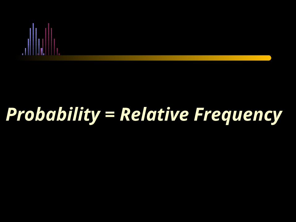
Typical Distribution for a Discrete Variable
Binomial Distribution (n=10, p=.50)
0
0.05
0.1
0.15
0.2
0.25
0.3
0 1 2 3 4 5 6 7 8 9 10
No. of Successes
Pro
bab
ilit
y
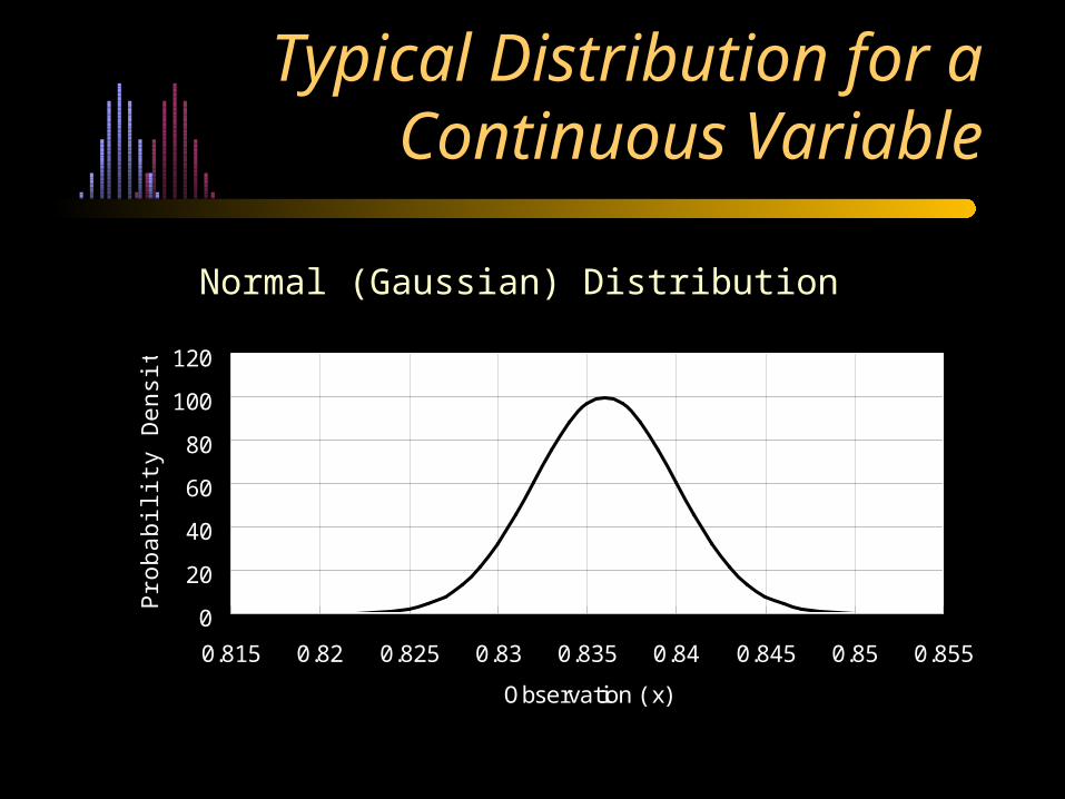
Typical Distribution for a Continuous Variable
0
20
40
60
80
100
120
0.815 0.82 0.825 0.83 0.835 0.84 0.845 0.85 0.855
Observation ( x)
Pro
ba
bili
ty D
en
sity
(f(
x))
Normal (Gaussian) Distribution
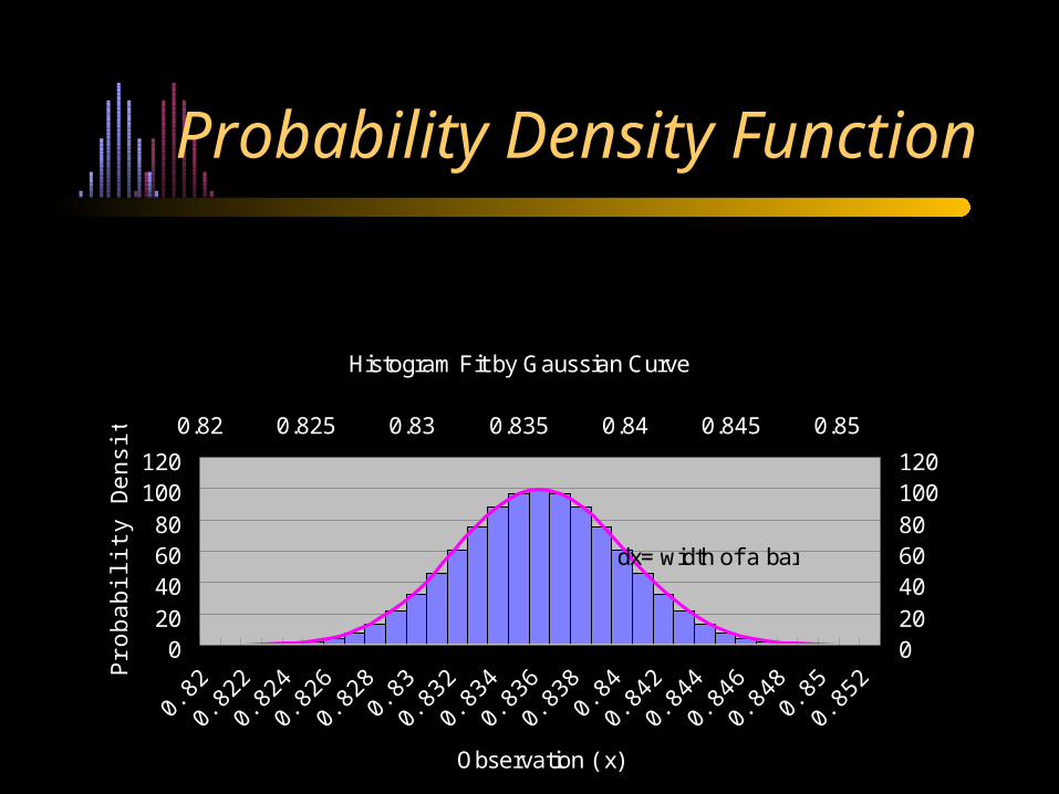
Probability Density Function
Histogram Fit by Gaussian Curve
020406080
100120
0.82
0.82
2
0.82
4
0.82
6
0.82
80.
83
0.83
2
0.83
4
0.83
6
0.83
80.
84
0.84
2
0.84
4
0.84
6
0.84
80.
85
0.85
2
Observation ( x)
Pro
ba
bili
ty D
en
sity
(f(
x))
020406080100120
0.82 0.825 0.83 0.835 0.84 0.845 0.85
dx= width of a bar
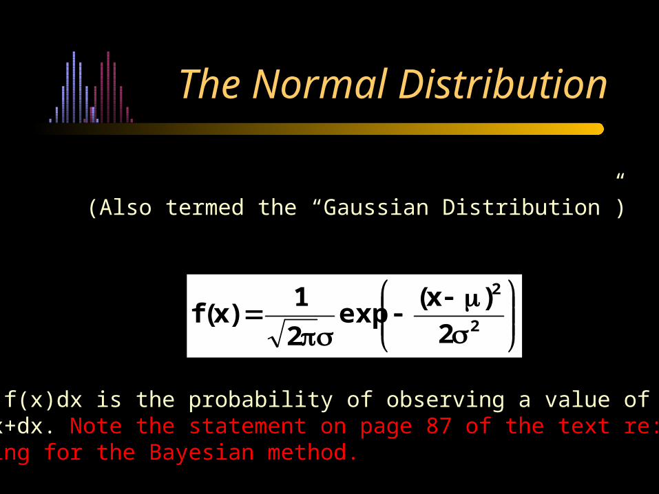
The Normal Distribution
2
2
2
)x(exp
2
1)x(f
(Also termed the “Gaussian Distribution”)
Note: f(x)dx is the probability of observing a value of x betweenx and x+dx. Note the statement on page 87 of the text re: dx canceling for the Bayesian method.
Selecting One Normal Distribution
The Normal Distribution can fit data with any mean and any standard deviation…..which one shall we focus on?
We do need to focus on just one….for tables and for theoretical developments.
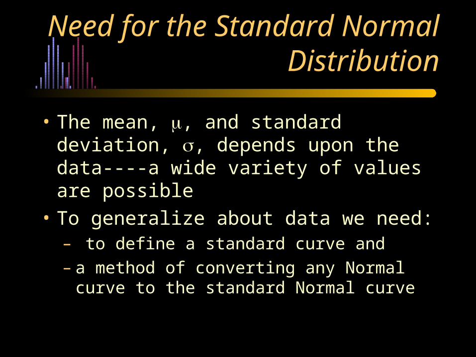
Need for the Standard Normal Distribution
• The mean, , and standard deviation, , depends upon the data----a wide variety of values are possible
• To generalize about data we need:– to define a standard curve and– a method of converting any Normal curve to
the standard Normal curve
The Standard Normal Distribution
= 0
= 1
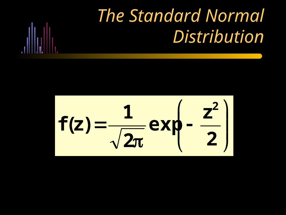
The Standard Normal Distribution
2
zexp
2
1)z(f
2
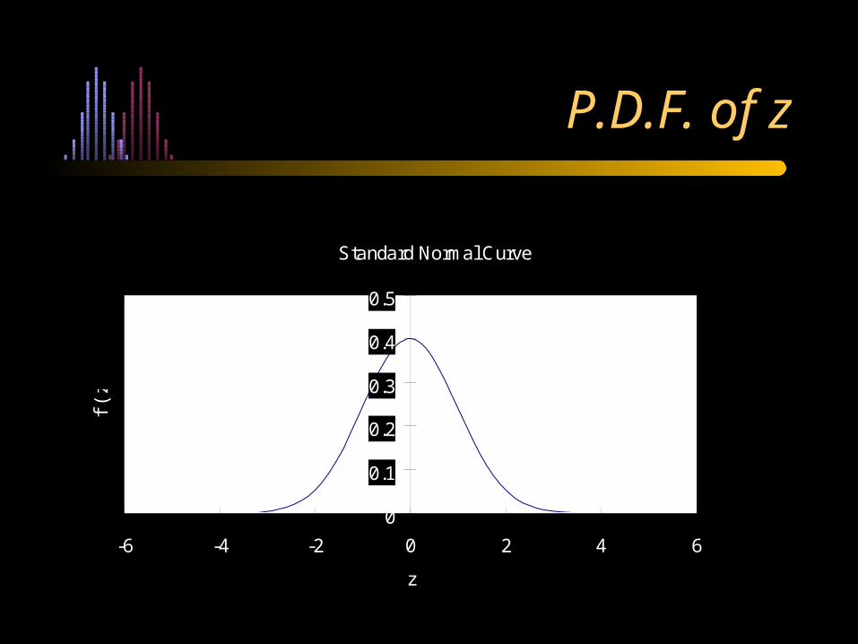
Standard Normal Curve
0
0.1
0.2
0.3
0.4
0.5
-6 -4 -2 0 2 4 6
z
f(z)
P.D.F. of z
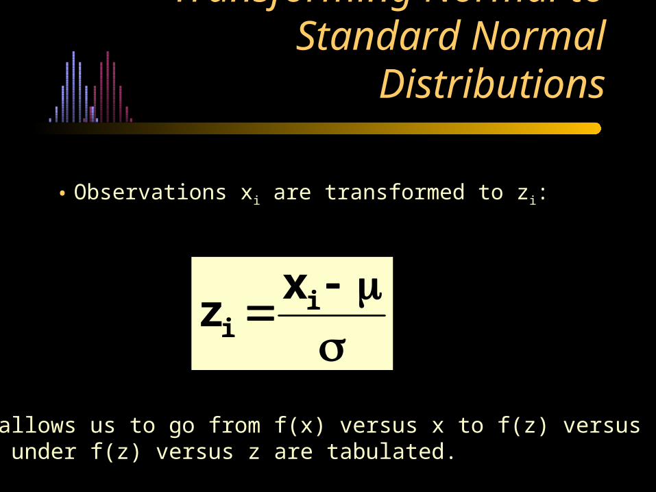
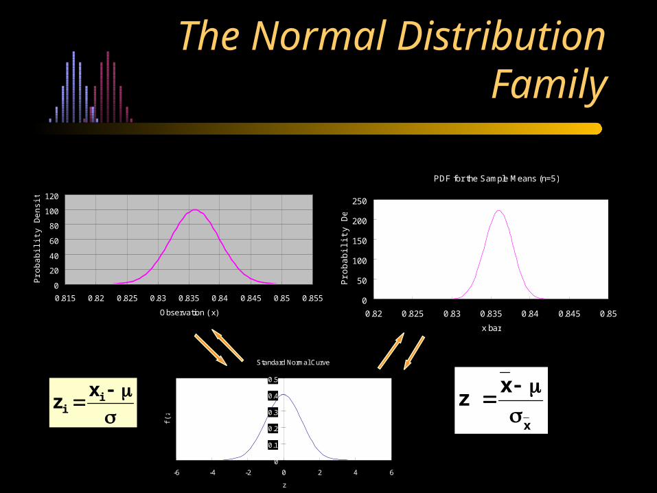
Transforming Normal to Standard Normal Distributions
• Observations xi are transformed to zi:
ii
xz
This allows us to go from f(x) versus x to f(z) versus z.Areas under f(z) versus z are tabulated.
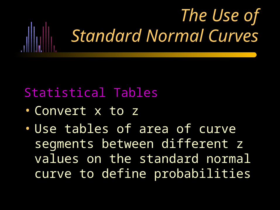
The Use of Standard Normal Curves
Statistical Tables
• Convert x to z
• Use tables of area of curve segments between different z values on the standard normal curve to define probabilities
Z Table
http://www.statsoft.com/textbook/stathome.html
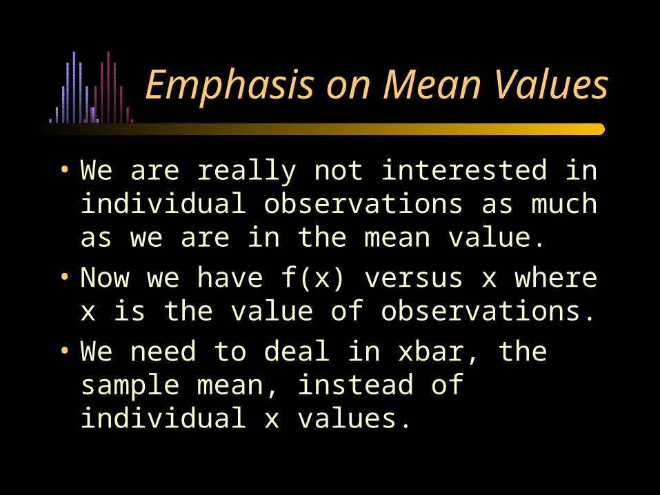
Emphasis on Mean Values
• We are really not interested in individual observations as much as we are in the mean value.
• Now we have f(x) versus x where x is the value of observations.
• We need to deal in xbar, the sample mean, instead of individual x values.
Introduction to Inferential Statistics
• Inferential statistics refers to methods for making generalizations about populations on the basis of data from samples
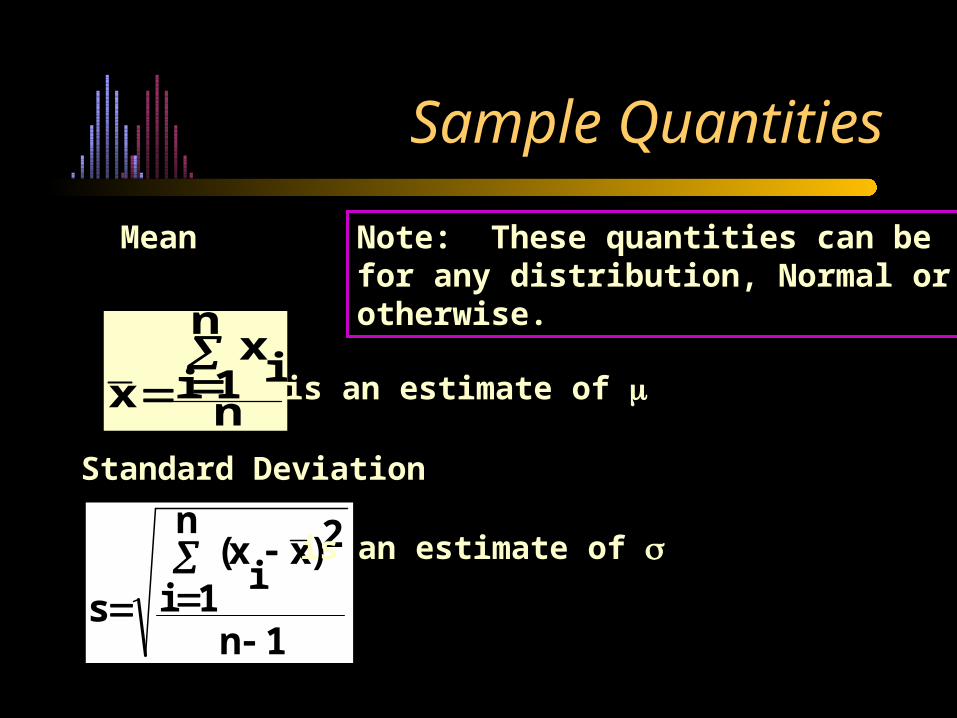
Sample Quantities
n
n
1i ix
x
1n
n
1i
2)xi
x(
s
Mean
Standard Deviation
is an estimate of
is an estimate of
Note: These quantities can befor any distribution, Normal orotherwise.
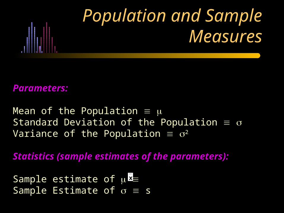
Population and Sample Measures
Parameters:
Mean of the Population Standard Deviation of the Population Variance of the Population 2
Statistics (sample estimates of the parameters):
Sample estimate of Sample Estimate of s
xx
x
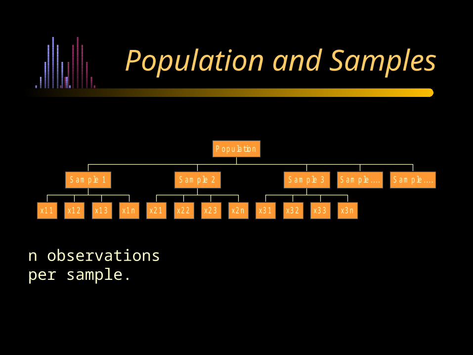
Population and Samples
x1 1 x1 2 x1 3 x1 n
S am p le 1
x2 1 x2 2 x2 3 x2 n
S am p le 2
x3 1 x3 2 x3 3 x3 n
S am p le 3 S am p le .... S am p le ....
P op u la tion
n observations per sample.

PDF for the Sample Means (n=5)
0
50
100
150
200
250
0.82 0.825 0.83 0.835 0.84 0.845 0.85
x bar
Pro
ba
bili
ty D
en
sity
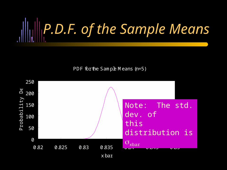
P.D.F. of the Sample Means
Note: The std. dev. of this distribution is xbar
Types of Estimators
• Point estimator - gives a single value as an estimate of the parameter of interest
• Interval estimator - specifies a range of values of the parameter and our confidence that the parameter value is in that range
Point Estimators
• Unbiased estimator: as the number of observations, n, increases for the sample the average value of the estimator approaches the value of the population parameter.
Interval Estimators
• P(lower limit<parameter<upper limit)
=1-• lower limit and upper limit = confidence
limits
• upper limit-lower limit=confidence interval
• 1- = confidence level; degree of confidence; confidence coefficient
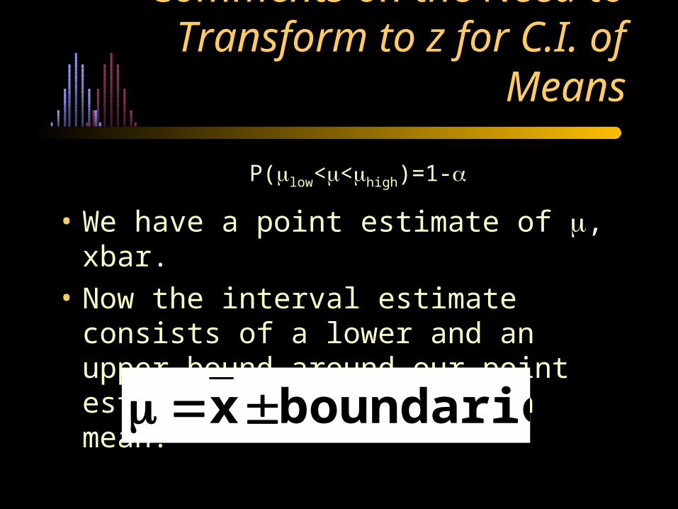
Comments on the Need to Transform to z for C.I. of Means
• We have a point estimate of , xbar.
• Now the interval estimate consists of a lower and an upper bound around our point estimate of the population mean:
P(low<<high)=1-
boundariesx
Confidence Interval for a Population Mean
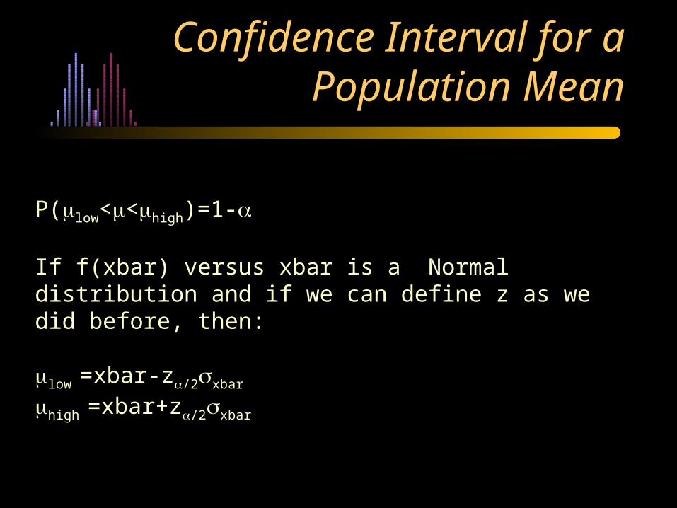
P(low<<high)=1-
If f(xbar) versus xbar is a Normal distribution and if we can define z as we did before, then:
low =xbar-z/2xbar
high =xbar+z/2xbar
A Standard Distribution for f(xbar) versus xbar
• Previously we transformed f(x) versus x to f(z) versus z
• We can still use f(z) versus z as our standard distribution.
• Now we need to transform f(xbar) versus xbar to f(z) versus z.
PDF for the Sample Means (n=5)
0
50
100
150
200
250
0.82 0.825 0.83 0.835 0.84 0.845 0.85
x bar
Pro
ba
bili
ty D
en
sity
P.D.F. of the Sample Means
Note: The std. dev. of this distribution is xbar

Standard Normal Curve
0
0.1
0.2
0.3
0.4
0.5
-6 -4 -2 0 2 4 6
z
f(z)
P.D.F. of z
Transforming Normal to Standard Normal Distributions
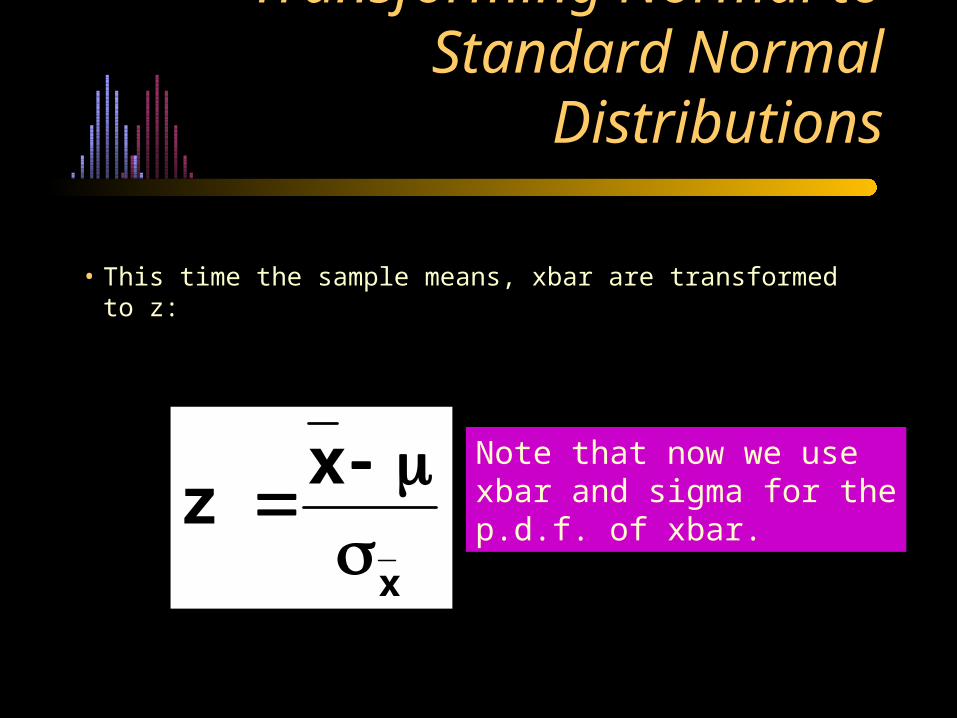
• This time the sample means, xbar are transformed to z:
x
xz
Note that now we use xbar and sigma for thep.d.f. of xbar.
0
20
40
60
80
100
120
0.815 0.82 0.825 0.83 0.835 0.84 0.845 0.85 0.855
Observation ( x)
Pro
ba
bili
ty D
en
sity
(f(
x))
The Normal Distribution Family
PDF for the Sample Means (n=5)
0
50
100
150
200
250
0.82 0.825 0.83 0.835 0.84 0.845 0.85
x bar
Pro
ba
bili
ty D
en
sity
Standard Normal Curve
0
0.1
0.2
0.3
0.4
0.5
-6 -4 -2 0 2 4 6
z
f(z)
x
xz
i
i
xz
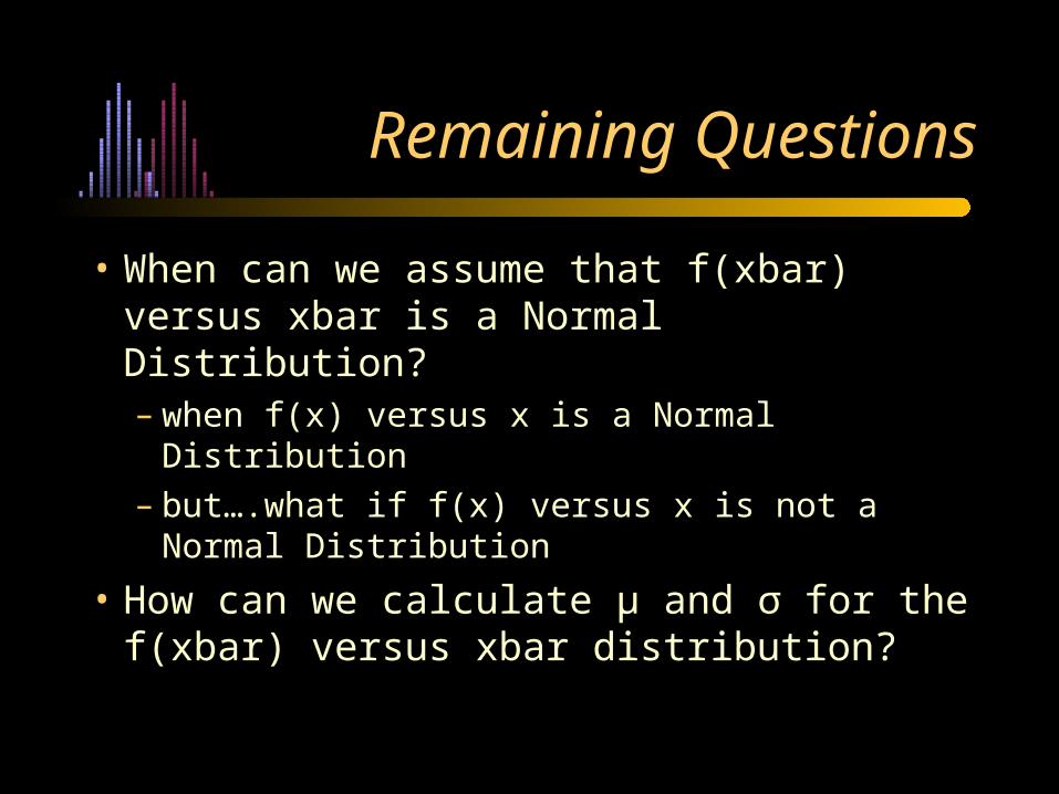
Remaining Questions
• When can we assume that f(xbar) versus xbar is a Normal Distribution?– when f(x) versus x is a Normal Distribution– but….what if f(x) versus x is not a Normal
Distribution
• How can we calculate μ and σ for the f(xbar) versus xbar distribution?
The Answer to Both Questions
The Central Limit Theorem
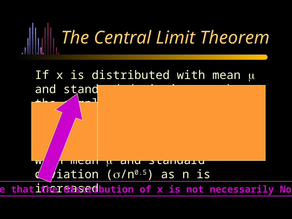
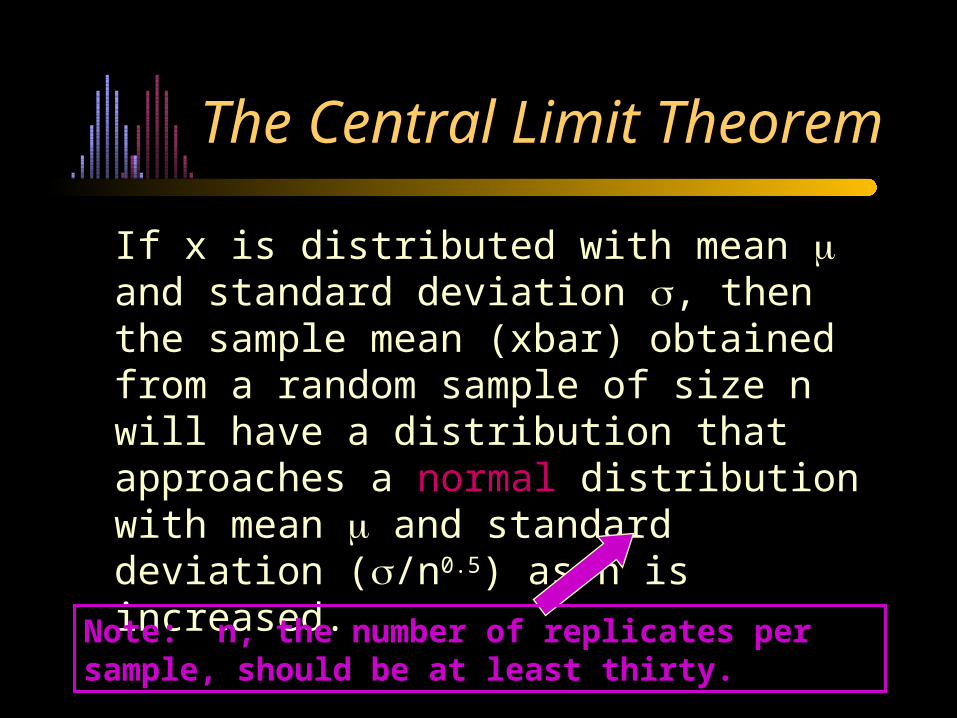
If x is distributed with mean and standard deviation , then the sample mean (xbar) obtained from a random sample of size n will have a distribution that approaches a normal distribution with mean and standard deviation (/n0.5) as n is increased
The Central Limit Theorem
Note that the distribution of x is not necessarily Normal.
The Central Limit Theorem
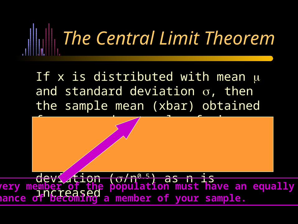
If x is distributed with mean and standard deviation , then the sample mean (xbar) obtained from a random sample of size n will have a distribution that approaches a normal distribution with mean and standard deviation (/n0.5) as n is increased
Every member of the population must have an equally likelychance of becoming a member of your sample.
The Central Limit Theorem
If x is distributed with mean and standard deviation , then the sample mean (xbar) obtained from a random sample of size n will have a distribution that approaches a normal distribution with mean and standard deviation (/n0.5) as n is increased
The Central Limit Theorem
If x is distributed with mean and standard deviation , then the sample mean (xbar) obtained from a random sample of size n will have a distribution that approaches a normal distribution with mean and standard deviation (/n0.5) as n is increased
The Central Limit Theorem
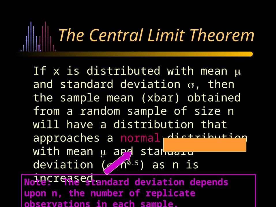
If x is distributed with mean and standard deviation , then the sample mean (xbar) obtained from a random sample of size n will have a distribution that approaches a normal distribution with mean and standard deviation (/n0.5) as n is increased.
Note: The standard deviation depends upon n, the number of replicate observations in each sample.
The Central Limit Theorem
If x is distributed with mean and standard deviation , then the sample mean (xbar) obtained from a random sample of size n will have a distribution that approaches a normal distribution with mean and standard deviation (/n0.5) as n is increased.
Note: n, the number of replicates per sample, should be at least thirty.
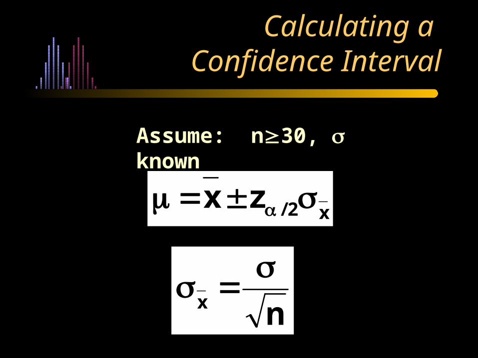
Calculating a Confidence Interval
x2/zx
nx
Assume: n30, known
Standard Normal Curve
0
0.1
0.2
0.3
0.4
0.5
-6 -4 -2 0 2 4 6
z
f(z)
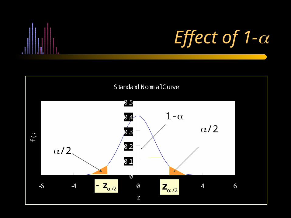
Effect of 1-
2/z
/21-
/2
2/z
Understanding What is a 95% Confidence Interval
• If we compute values of the confidence interval with many different random samples from the same population, then in about 95% of those samples, the value of the 95% c.i. so calculated would include the value of the population mean, .
• Note that is a constant.
• The c.i. vary because they are each based on a sample.
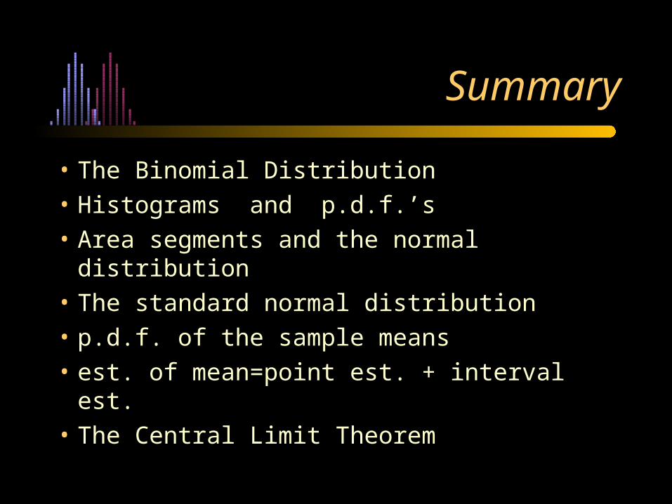
• The Binomial Distribution
• Histograms and p.d.f.’s
• Area segments and the normal distribution
• The standard normal distribution
• p.d.f. of the sample means
• est. of mean=point est. + interval est.
• The Central Limit Theorem
Summary
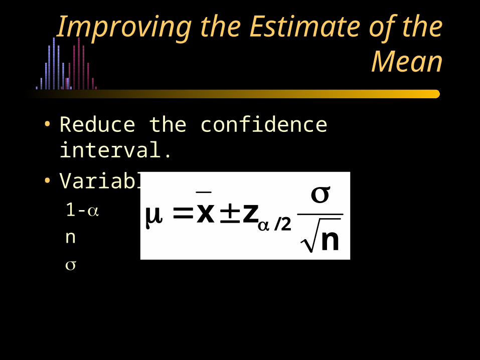
Improving the Estimate of the Mean
• Reduce the confidence interval.
• Variables to examine:1-n
nzx 2/
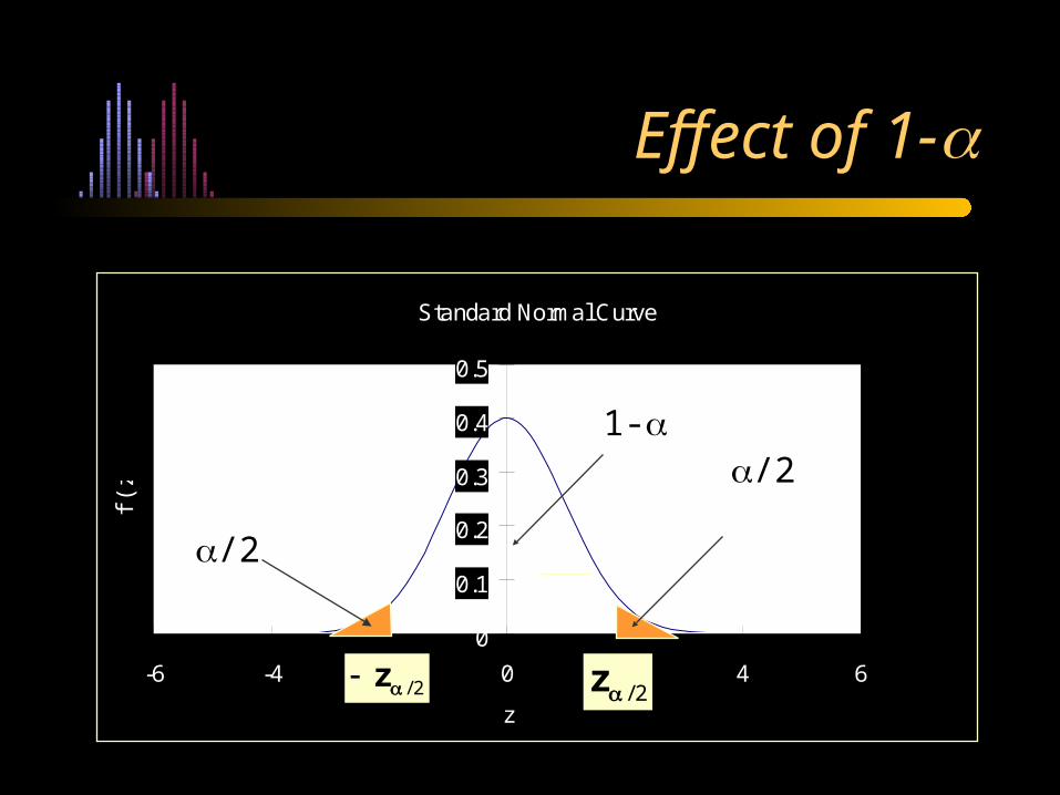
Standard Normal Curve
0
0.1
0.2
0.3
0.4
0.5
-6 -4 -2 0 2 4 6
z
f(z)
Effect of 1-
2/z
/21-
/2
2/z
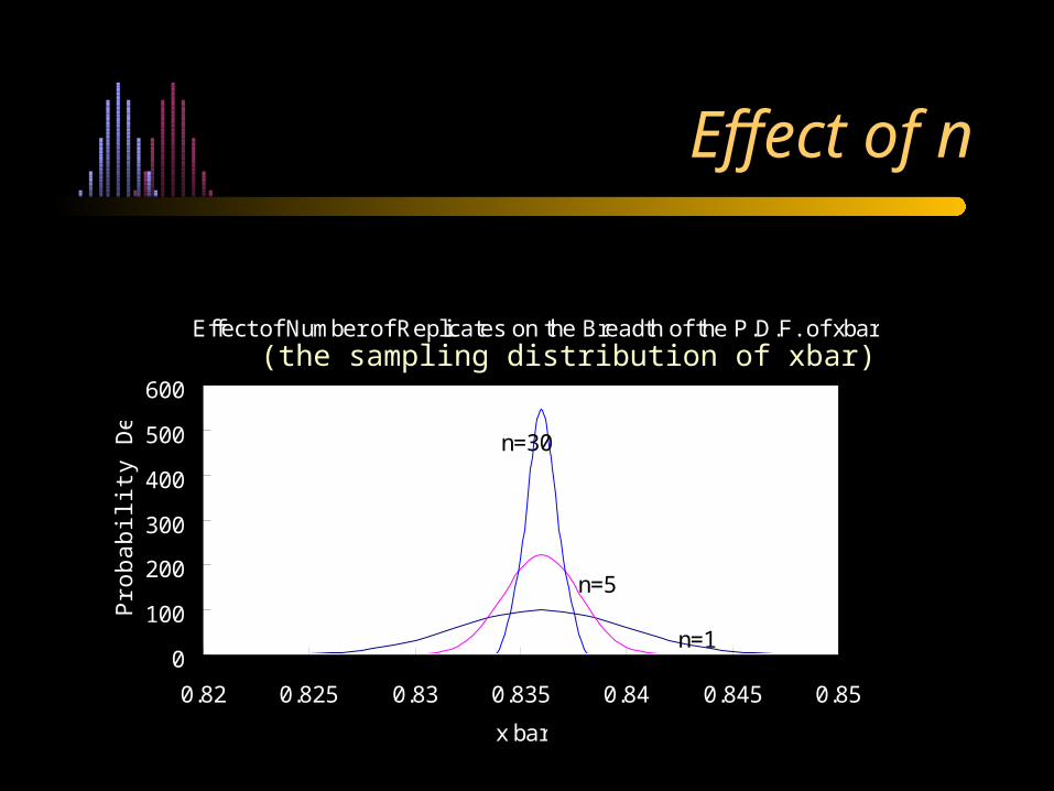
Effect of Number of Replicates on the Breadth of the P.D.F. of xbar
0
100
200
300
400
500
600
0.82 0.825 0.83 0.835 0.84 0.845 0.85
x bar
Pro
ba
bili
ty D
en
sity
n=1
n=30
n=5
Effect of n
(the sampling distribution of xbar)
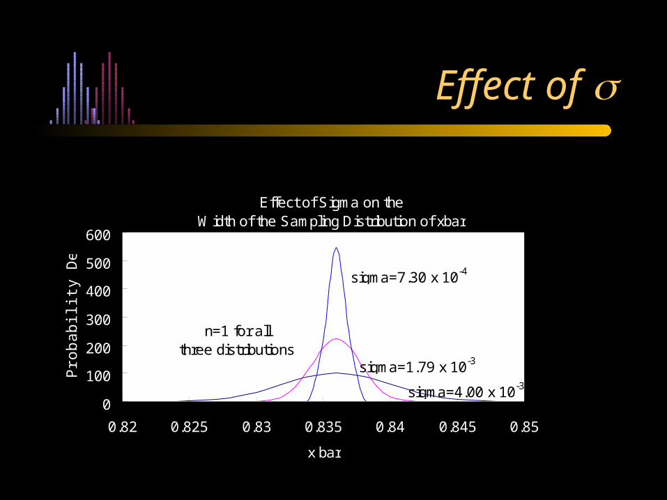
Effect of
Effect of Sigma on the Width of the Sampling Distribution of xbar
0
100
200
300
400
500
600
0.82 0.825 0.83 0.835 0.84 0.845 0.85
x bar
Pro
ba
bili
ty D
en
sity
sigma=4.00 x 10⁻³
sigma=7.30 x 10⁻⁴
sigma=1.79 x 10⁻³
n=1 for all three distributions
Understanding the Question
• If we are asked to estimate the value of the population mean then we provide:– the point estimate + the interval estimate of the
mean
• If we are asked to estimate the noise in the experimental technique then we provide:– the point estimate + the interval estimate of the
standard deviation (something not reviewed yet)
Complication for Small Samples
• For small samples (n<30), if the observations, x, follow a Normal distribution, and if must be approximated by s, then the sample means, xbar, tend to follow a “Student’s t” distribution rather than a Normal distribution.
• So, we must use t instead of z.
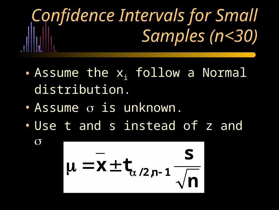
Confidence Intervals for Small Samples (n<30)
• Assume the xi follow a Normal distribution.
• Assume is unknown.
• Use t and s instead of z and
n
stx 1n,2/
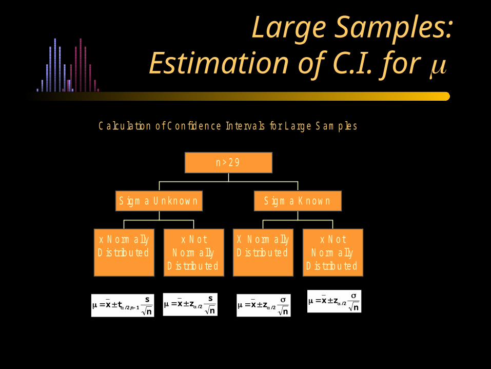
Large Samples:Estimation of C.I. for
C alcu la tion o f C on fid en ce In te rva ls fo r L arg e S am p les
x N orm a llyD is trib u ted
x N otN orm ally
D is trib u ted
S ig m a U n kn ow n
X N orm allyD is trib u ted
x N otN orm ally
D is trib u ted
S ig m a K n ow n
n > 2 9
n
stx 1n,2/ n
zx 2/
n
szx 2/
nzx 2/
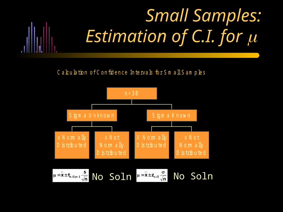
Small Samples:Estimation of C.I. for
C alcu la tion o f C on fid en ce In te rva ls fo r S m a ll S am p les
x N orm a llyD is trib u ted
x N otN orm a lly
D is trib u ted
S ig m a U n kn ow n
X N orm allyD is trib u ted
x N otN orm a lly
D is trib u ted
S ig m a K n ow n
n < 3 0
n
stx 1n,2/
nzx 2/
No Soln No Soln
Return to a Data Mining Problem
• Predicting Classifier Performance…..
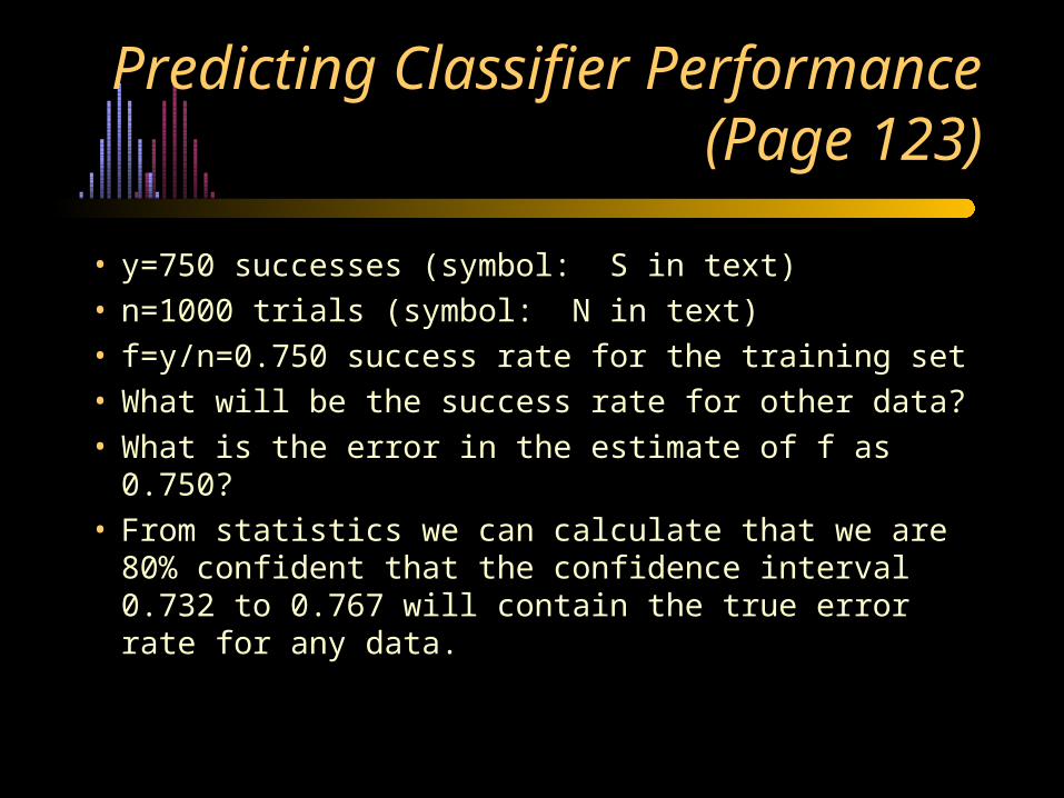
Predicting Classifier Performance (Page 123)
• y=750 successes (symbol: S in text)• n=1000 trials (symbol: N in text)• f=y/n=0.750 success rate for the training set• What will be the success rate for other data?• What is the error in the estimate of f as 0.750?• From statistics we can calculate that we are 80%
confident that the confidence interval 0.732 to 0.767 will contain the true error rate for any data.
The Binomial Distribution
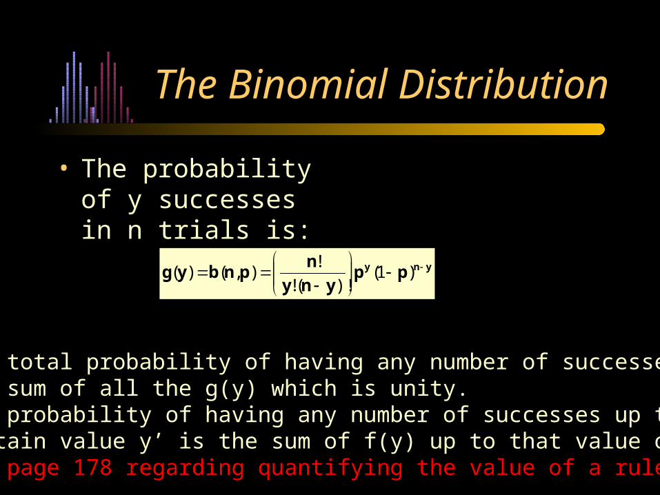
• The probability of y successes in n trials is:
yny ppyny
npnbyg
)1()!(!
!),()(
The total probability of having any number of successes isthe sum of all the g(y) which is unity.The probability of having any number of successes up to a certain value y’ is the sum of f(y) up to that value of y.See page 178 regarding quantifying the value of a rule.
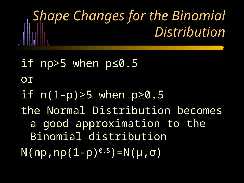
Shape Changes for the Binomial Distribution
if np>5 when p≤0.5
or
if n(1-p)≥5 when p≥0.5
the Normal Distribution becomes a good approximation to the Binomial distribution
N(np,np(1-p)0.5)=N(μ,σ)
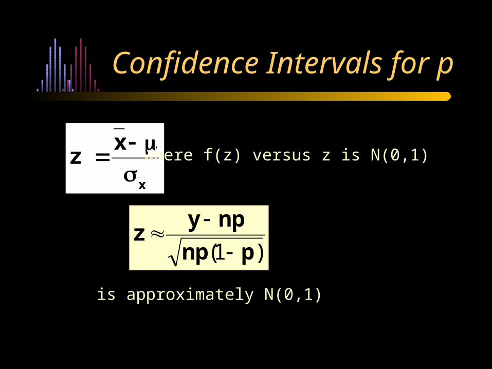
Confidence Intervals for p
)1( pnp
npyz
is approximately N(0,1)
x
xz
where f(z) versus z is N(0,1)
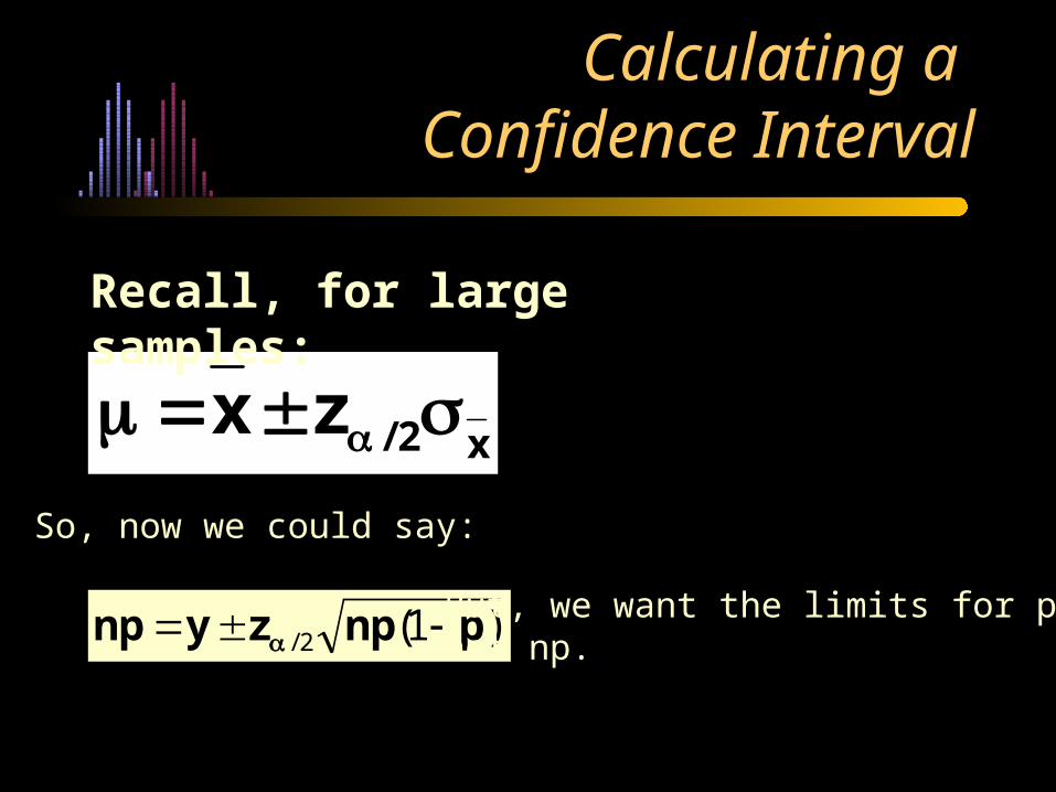
Calculating a Confidence Interval
x2/zx
Recall, for large samples:
So, now we could say:
)1(2/ pnpzynp But, we want the limits for p,not np.
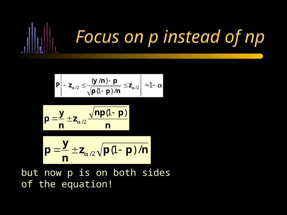
Focus on p instead of np
nppzn
yp /)1(2/
n
pnpz
n
yp
)1(2/
but now p is on both sidesof the equation!
1/)1(
)/(2/2/ z
npp
pnyzP
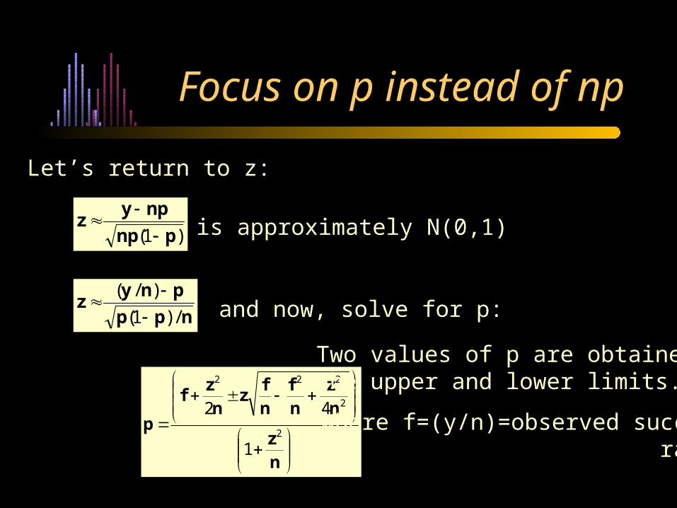
Focus on p instead of np
)1( pnp
npyz
npp
pnyz
/)1(
)/(
is approximately N(0,1)
Let’s return to z:
and now, solve for p:
nz
nz
nf
nf
zn
zf
p2
2
222
1
42where f=(y/n)=observed success rate
Two values of p are obtained:the upper and lower limits.
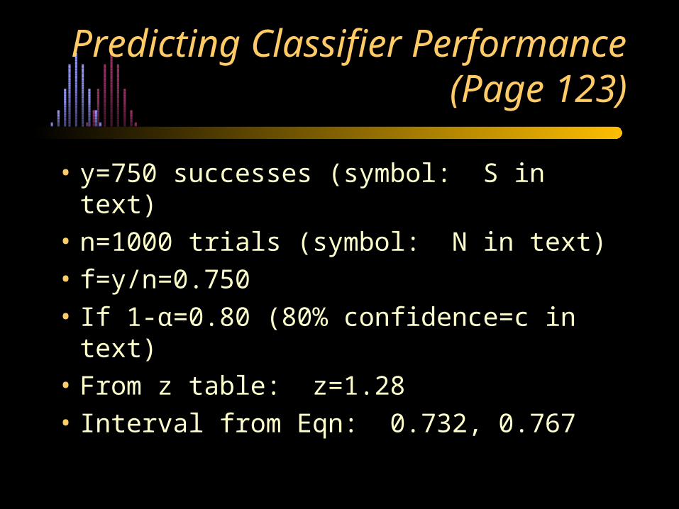
Predicting Classifier Performance (Page 123)
• y=750 successes (symbol: S in text)
• n=1000 trials (symbol: N in text)
• f=y/n=0.750
• If 1-α=0.80 (80% confidence=c in text)
• From z table: z=1.28
• Interval from Eqn: 0.732, 0.767
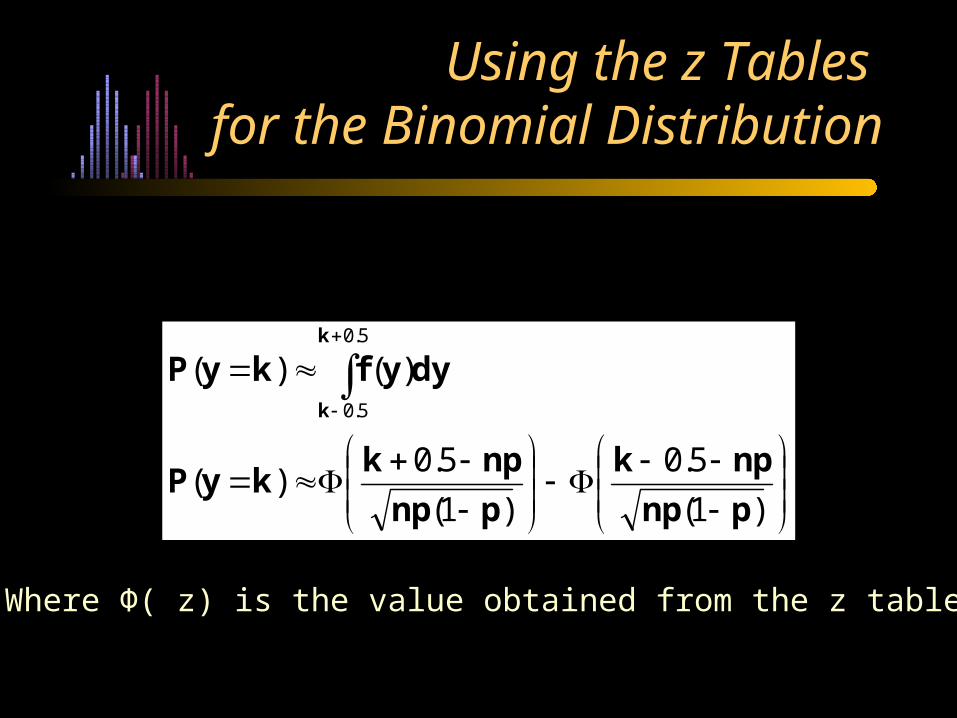
Using the z Tables for the Binomial Distribution
)1(
5.0
)1(
5.0)(
)()(5.0
5.0
pnp
npk
pnp
npkkyP
dyyfkyPk
k
Where Φ( z) is the value obtained from the z table.
• The Binomial Distribution• Histograms and p.d.f.’s• Area segments and the normal distribution• The standard normal distribution • p.d.f. of the sample means• est. of mean=point est. + interval est.• The Central Limit Theorem• Confidence Intervals
Summary
In Two Weeks
• Hypothesis Testing:How do we know if we can accept a batch of
material from a few replicate analyses of a sample?
Are the error rates obtained from two data mining methods really different?