STATISTICS: AN INTRODUCTION USING R

By M.J. Crawley

Exercises

10. ANALYSING PROPORTION DATA: BINOMIAL ERRORS An important class of problems involves data on proportions: • data on percentage mortality • infection rates of diseases • proportion responding to clinical treatment • proportion admitting to particular voting intentions • data on proportional response to an experimental treatment What all these have in common is that we know how many of the experimental objects are in one category (say dead, insolvent or infected) and we know how many are in another (say alive, solvent or uninfected). This contrasts with Poisson count data, where we knew how many times an event occurred, but not how many times it did not occur. We model processes involving proportional response variables in S-Plus by specifying a glm with family=binomial . The only complication is that whereas with Poisson errors (Practical 11) we could simply say family=poisson, with binomial errors we must specify the number of failures as well as the numbers of successes in a 2-vector response variable. To do this we bind together two vectors using cbind into a single object, y, comprising the numbers of successes and the number of failures. The binomial denominator, n, is the total sample, and the

number.of.failures = binomial.denominator – number.of.successes

y <- cbind( number.of.successes, number.of.failures) The old fashioned way of modelling this sort of data was to use the percentage mortality as the response variable. There are 3 problems with this: • the errors are not normally distributed • the variance is not constant • by calculating the percentage, we lose information of the size of the sample, n,

from which the proportion was estimated In S-Plus, we use the number responding and the number not responding bound together as the response variable. S-Plus then carries out weighted regression, using the individual sample sizes as weights, and the logit link function to ensure linearity (as described below).

If the response variable takes the form of a percentage change in some continuous measurement (such as the percentage change in weight on receiving a particular diet), then the data should be arc-sine transformed prior to analysis, especially if many of the percentage changes are smaller than 20% or larger than 80%. Note, however, that data of this sort are probably better treated by either • analysis of covariance (see Practical 6), using final weight as the response variable

and initial weight as a covariate • or by specifying the response variable to be a relative growth rates, where the

response variable is ln(final weight/initial weight). There are some proportion data, like percentage cover, which are best analysed using conventional models (normal errors and constant variance) following arc-sine transformation. The response variable, y, measured in radians, is p×− 01.0sin 1 where p is cover in %. Count data on proportions The traditional transformations of proportion data were arcsine and probit. The arcsine transformation took care of the error distribution, while the probit transformation was used to linearize the relationship between percentage mortality and log dose in a bioassay. There is nothing wrong with these transformations, and they are available within S-Plus, but a simpler approach is often preferable, and is likely to produce a model that is easier to interpret. The major difficulty with modelling proportion data is that the responses are strictly bounded. There is no way that the percentage dying can be greater than 100% or less than 0%. But if we use simple techniques like regression or analysis of covariance, then the fitted model could quite easily predict negative values, especially if the variance was high and many of the data were close to 0. The logistic curve is commonly used to describe data on proportions, because, unlike the straight line model, it asymptotes at 0 and 1 so that negative proportions, and responses of more than 100% can not be predicted. Throughout this discussion we shall use p to describe the proportion of individuals observed to respond in a given way. Because much of their jargon was derived from the theory of gambling, statisticians call these successes although, to an ecologist measuring death rates this may seem somewhat macabre. The individuals that respond in other ways (the statistician's failures) are therefore (1-p) and we shall call the proportion of failures q. The third variable is the size of the sample, n, from which p was estimated (it is the binomial denominator, and the statistician's number of attempts). An important point about the binomial distribution is that the variance is not constant. In fact, the variance of the binomial distribution is:

s npq2 = so that the variance changes with the mean like this:

p

s2

0.0 0.2 0.4 0.6 0.8 1.0

0.0

0.05

0.10

0.15

0.20

0.25

The variance is low when p is very high or very low, and the variance is greatest when p = q = 0.5. As p gets smaller, so the binomial distribution gets closer and closer to the Poisson distribution. You can see why this is so by considering the formula for the variance of the binomial: s2 = npq. Remember that for the Poisson, the variance is equal to the mean; s2 = np. Now, as p gets smaller, so q gets closer and closer to 1, so the variance of the binomial converges to the mean:

s npq np q2 1= ≈ ≈ ( ) Odds The logistic model for p as a function of x looks like this:

pe

e

a bx

a bx=+

+

+

( )

( )1

and there are no prizes for realising that the model is not linear. But if x = , then p=0; if x = +∞ then p=1 so the model is strictly bounded. When x = 0 then p = exp(a)/(1 + exp(a)). The trick of linearising the logistic actually involves a very simple transformation. You may have come across the way in which bookmakers specify probabilities by quoting the odds against a particular horse winning a race (they might give odds of 2 to 1 on a reasonably good horse or 25 to 1 on an outsider). This is a rather different way of presenting information on probabilities than scientists are used to dealing with. Thus, where the scientist might state a proportion as 0.666 (2 out of 3), the bookmaker would give odds of 2 to 1 (2 successes to 1 failure). In symbols, this is the difference between the scientist stating the probability p, and the bookmaker stating the odds, p/q. Now if we take the odds p/q and substitute this into the formula for the logistic, we get:

− ∞

pq

ee

ee

a bx

a bx

a bx

a bx=+

−+

⎡

⎣⎢

⎤

⎦⎥

+

+

+

+

−( )

( )

( )

( )11

1

1

which looks awful. But a little algebra shows that:

pq

ee e

ea bx

a bx a bxa bx=

+ +⎡⎣⎢

⎤⎦⎥

=+

+ +

−+

( )

( ) ( )( )

11

1

1

Now, taking natural logs, and recalling that ln( will simplify matters even further, so that

)ex = x

lnpq

a bx⎛⎝⎜

⎞⎠⎟ = +

This gives a linear predictor, a + bx, not for p but for the logit transformation of p, namely ln(p/q). In the jargon of SPlus, the logit is the link function relating the linear predictor to the value of p.

You might ask at this stage 'why not simply do a linear regression of ln(p/q) against the explanatory x-variable'? SPlus has three great advantages here: • it allows for the non-constant binomial variance; • it deals with the fact that logits for p's near 0 or 1 are infinite; • it allows for differences between the sample sizes by weighted regression. Deviance with binomial errors Before we met glm’s we always used SSE as the measure of lack of fit (see p. xxx). For data on proportions, the maximum likelihood estimate of lack of fit is different from this: if y is the observed count and is the fitted value predicted by the current $y

model, then if n is the binomial denominator (the sample size from which we obtained y successes), the deviance is :

2 yyy

n yn yn y

log$

( ) log( )( $)

⎡

⎣⎢

⎤

⎦⎥ + −

−−

⎡

⎣⎢

⎤

⎦⎥∑

We should try this on a simple numerical example. In a trial with two treatments and two replicates per treatment we got 3 out of 6 and 4 out of 10 in one treatment, and 5 out of 9 and 8 out of 12 in the other treatment. Are the proportions significantly different across the two treatments? One thing you need to remember is how to calculate the average of two proportions. You don’t work out the two proportions, add them up and divide by 2. What you do is count up the total number of successes and divide by the total number of attempts. In our case, the overall mean proportion is calculated like this. The total number of successes, y, is (3 + 4 + 5 + 8) = 20. The total number of attempts, N, is (6 + 10 + 9 + 12) = 37. So the overall average proportion is 20/37 = 0.5405. We need to work out the 4 expected counts. We multiply each of the sample sizes by the mean proportion: 6 x 0.5405 etc. y<-c(3,4,5,8) N<-c(6,10,9,12) N*20/37 [1] 3.243243 5.405405 4.864865 6.486486 Now we can calculate the total deviance:

⎭⎬⎫

⎩⎨⎧

⎟⎠⎞

⎜⎝⎛

−+⎟

⎠⎞

⎜⎝⎛+⎟

⎠⎞

⎜⎝⎛

−+⎟

⎠⎞

⎜⎝⎛+⎟

⎠⎞

⎜⎝⎛

−+⎟

⎠⎞

⎜⎝⎛+⎟

⎠⎞

⎜⎝⎛

−+⎟

⎠⎞

⎜⎝⎛×

486.6124log4

486.68log8

865.494log4

865.45log5

405.5106log6

405.54log4

243.363log3

243.33log32

You wouldn’t want to have to do this too often, but it is worth it to demystify deviance. p1<-2*(3*log(3/3.243)+3*log(3/(6-3.243))+4*log(4/5.405)+6*log(6/(10-5.405))) p2<-2*(5*log(5/4.865)+4*log(4/(9-4.865))+8*log(8/6.486)+4*log(4/(12-6.486))) p1+p2 [1] 1.629673 So the total deviance is 1.6297. Let’s see what a glm with binomial errors gives: rv<-cbind(y,N-y) glm(rv~1,family=binomial) Degrees of Freedom: 3 Total (i.e. Null); 3 Residual Null Deviance: 1.63 Residual Deviance: 1.63 AIC: 14.28

Great relief all round. What about the residual deviance? We need to compute a new set of fitted values based on the two individual treatment means. Total successes in treatment A were 3 + 4 = 7 out of a total sample of 6 + 10 = 16. So the mean proportion was 7/16 = 0.4375. In treatment B the equivalent figures were 13/21 = 0.619. So the fitted values are p<-c(7/16,7/16,13/21,13/21) p*N [1] 2.625000 4.375000 5.571429 7.428571 and the residual deviance is

⎭⎬⎫

⎩⎨⎧

⎟⎠⎞

⎜⎝⎛

−+⎟

⎠⎞

⎜⎝⎛+⎟

⎠⎞

⎜⎝⎛

−+⎟

⎠⎞

⎜⎝⎛+⎟

⎠⎞

⎜⎝⎛

−+⎟

⎠⎞

⎜⎝⎛+⎟

⎠⎞

⎜⎝⎛

−+⎟

⎠⎞

⎜⎝⎛×

429.7124log4

429.78log8

571.594log4

571.55log5

375.4106log6

375.44log4

625.263log3

625.23log32

Again, we calculate this in 2 parts p1<-2*(3*log(3/2.625)+3*log(3/(6-2.625))+4*log(4/4.375)+6*log(6/(10-4.375))) p2<-2*(5*log(5/5.571)+4*log(4/(9-5.571))+8*log(8/7.429)+4*log(4/(12-7.429))) p1+p2 [1] 0.4201974 treatment<-factor(c("A","A","B","B")) glm(rv~treatment,family=binomial) Degrees of Freedom: 3 Total (i.e. Null); 2 Residual Null Deviance: 1.63 Residual Deviance: 0.4206 AIC: 15.07 So there really is no mystery in the values of deviance. It is just another way of measuring lack of fit. The difference between 0.4201974 and 0.4206 is just due to our use of only 3 decimal places in calculating the deviance components. If you were perverse, you could always work it out for yourself. Everything we have done with sums of squares (e.g. F tests and r2), you can do with deviance. S-Plus commands for Proportional Data In addition to specifying that the y-variable contains the counted data on the number of successes, SPlus requires the user to provide a second vector containing the number of failures. The response is then a 2-column data frame, y, produced like this:

y <- cbind(successes,failures) The sum of the successes and failures is the binomial denominator (the size of the sample from which each trial was drawn). This is used as a weight in the statistical modelling.

Overdispersion and hypothesis testing All the different statistical procedures that we have met in earlier chapters can also be used with data on proportions. Factorial analysis of variance, multiple regression, and a variety of mixed models in which different regression lines are fit in each of several levels of one or more factors, can be carried out. The only difference is that we assess the significance of terms on the basis of chi-squared; the increase in scaled deviance that results from removal of the term from the current model. The important point to bear in mind is that hypothesis testing with binomial errors is less clear-cut than with normal errors. While the chi squared approximation for changes in scaled deviance is reasonable for large samples (i.e. bigger than about 30), it is poorer with small samples. Most worrisome is the fact that the degree to which the approximation is satisfactory is itself unknown. This means that considerable care must be exercised in the interpretation of tests of hypotheses on parameters, especially when the parameters are marginally significant or when they explain a very small fraction of the total deviance. With binomial or Poisson errors we can not hope to provide exact P-values for our tests of hypotheses. As with Poisson errors, we need to address the question of overdispersion (see Practical 11). When we have obtained the minimal adequate model, the residual scaled deviance should be roughly equal to the residual degrees of freedom. When the residual deviance is larger than the residual degrees of freedom there are two possibilities: either the model is mis-specified, or the probability of success, p, is not constant within a given treatment level. The effect of randomly varying p is to increase the binomial variance from npq to

s npq n n2 21= + −( )σ leading to a large residual deviance. This occurs even for models that would fit well if the random variation were correctly specified. One simple solution is to assume that the variance is not but , where s is an unknown scale parameter (s > 1). We obtain an estimate of the scale parameter by dividing the Pearson chi-square by the degrees of freedom, and use this estimate of s to compare the resulting scaled deviances for terms in the model using an F test (just as in conventional anova, Practical 5). While this procedure may work reasonably well for small amounts of overdispersion, it is no substitute for proper model specification. For example, it is not possible to test the goodness of fit of the model.

npq npqs

Model Criticism Next, we need to assess whether the standardised residuals are normally distributed and whether there are any trends in the residuals, either with the fitted values or with the explanatory variables. It is necessary to deal with standardised residuals because with error distributions like the binomial, Poisson or gamma distributions, the variance changes with the mean. To obtain plots of the standardised residuals, we need to calculate:

ry

Vy

bd

s =−

=−

−⎛⎝⎜

⎞⎠⎟

µ µ

µµ

1

where V is the formula for the variance function of the binomial, µ are the fitted values, and bd is the binomial denominator (successes plus failures). Other kinds of standardised residuals (like Pearson residuals or deviance residuals) are available as options like this:

resid(model.name, type = “pearson” )

or you could use other types including “deviance”, “working” or “response”. To plot the residuals against the fitted values, we might arc-sine transform the x axis (because the fitted data are proportions): Summary The most important points to emphasise in modelling with binomial errors are: • create a 2-column object for the response, using cbind to join together the two

vectors containing the counts of success and failure • check for overdispersion (residual deviance > residual degrees of freedom), and

correct for it by using F tests rather than chi square if necessary • remember that you do not obtain exact P-values with binomial errors; the chi

squared approximations are sound for large samples, but small samples may present a problem

• the fitted values are counts, like the response variable • the linear predictor is in logits (the log of the odds = p/q) • you can back transform from logits (z) to proportions (p) by p = 1/(1+1/exp(z)) Applications 1) Regression analysis with proportion data In a study of density dependent seed mortality in trees, seeds were placed in 6 groups of different densities (size from 4 to 100). The scientist returned after 48 hours and counted the number of seeds taken away by animals. We are interested to see if the proportion of seeds taken is influenced by the size of the cache of seeds. These are the data: taken<-c(3,3,6,16,26,39) size<-c(4,6,10,40,60,100) Now calculate the proportion removed (p) and the logarithm of pile size (ls):

p<-taken/size ls<-log(size) plot(ls,p) abline(lm(p~ls))

It certainly looks as if the proportion taken declines as density increases. Let’s do the regression to test the significance of this: summary(lm(p~ls)) Call: lm(formula = p ~ ls) Residuals: 1 2 3 4 5 6 0.09481 -0.11877 0.02710 -0.04839 0.02135 0.02390 Coefficients: Estimate Std. Error t value Pr(>|t|) (Intercept) 0.77969 0.08939 8.723 0.000952 *** ls -0.08981 0.02780 -3.230 0.031973 * Residual standard error: 0.08246 on 4 degrees of freedom Multiple R-Squared: 0.7229, Adjusted R-squared: 0.6536 F-statistic: 10.43 on 1 and 4 degrees of freedom, p-value: 0.03197 So the density dependent effect is significant (p = 0.032). But these were proportion data. Perhaps we should have transformed them before doing the regression ? We can repeat the regression using the logit transformation.

logit<-log(p/(1-p)) summary(lm(logit~ls)) Call: lm(formula = logit ~ ls) Residuals: 1 2 3 4 5 6 0.43065 -0.51409 0.08524 -0.19959 0.09149 0.10630 Coefficients: Estimate Std. Error t value Pr(>|t|) (Intercept) 1.1941 0.3895 3.065 0.0375 * ls -0.3795 0.1212 -3.132 0.0351 * Residual standard error: 0.3593 on 4 degrees of freedom Multiple R-Squared: 0.7104, Adjusted R-squared: 0.638 F-statistic: 9.811 on 1 and 4 degrees of freedom, p-value: 0.03511 The regression is still significant, suggesting density dependence in removal rate. Now we shall carry out the analysis properly, taking account of the fact that the very high death rates were actually estimated from very small samples of seeds (4, 6, and 10 individuals respectively). A glm with binomial errors takes care of this by giving low weight to estimates with small binomial denominators. First we need to construct a response vector (using cbind) that contains the number of successes and the number of failures. In our example, this means the number of seeds taken away and the number of seeds left behind. We do it like this: left<-size - taken y<-cbind(taken,left) Now the modelling. We use glm instead of lm, but otherwise everything else is the same as usual. model<-glm(y~ls,binomial) summary(model) Call: glm(formula = y ~ ls, family = binomial) Deviance Residuals: [1] 0.5673 -0.4324 0.3146 -0.6261 0.2135 0.1317 Coefficients: Estimate Std. Error z value Pr(>|z|) (Intercept) 0.8815 0.7488 1.177 0.239 ls -0.2944 0.1817 -1.620 0.105

(Dispersion parameter for binomial family taken to be 1) Null deviance: 3.7341 on 5 degrees of freedom Residual deviance: 1.0627 on 4 degrees of freedom AIC: 25.543 When we do the analysis properly, using weighted regression in glim, we see that there is no significant effect of density on the proportion of seeds removed (p = 0.105). This analysis was carried out by a significance test on the parameter values. It is usually better to assess significance by a deletion test. To do this, we fit a simpler model with an intercept but no slope: model2<-glm(y~1,binomial) anova(model,model2) Analysis of Deviance Table Response: y Resid. Df Resid. Dev Df Deviance ls 4 1.0627 1 5 3.7341 -1 -2.6713 The thing to remember is that the change in deviance is a chi squared value. In this case the chi-square on 1 d.f. is only 2.671 and this is less than the value in tables (3.841), so we conclude that there is no evidence for density dependence in the death rate of these seeds. It is usually more convenient to have the chi squared test printed out as part of the analysis of deviance table. This is very straightforward. We just include the option test=”Chi” in the anova directive anova(model,model2,test="Chi") Analysis of Deviance Table Response: y Resid. Df Resid. Dev Df Deviance P(>|Chi|) ls 4 1.0627 1 5 3.7341 -1 -2.6713 0.1022 The moral is clear. Tests of density dependence need to be carried out using weighted regression, so that the death rates estimated from small samples do not have undue influence on the value of the regression slope. In this example, using the correct linearization technique (logit transformation) did not solve the problem; logit regression agreed (wrongly) with simple regression that there was significant inverse density dependence (i.e. the highest death rates were estimated at the lowest densities). But these high rates were estimated from tiny samples (3 out of 4 and 3 out of 6 individuals). The correct analysis uses weighted regression and binomial errors, in which case these points are given less influence. The result is that the data no longer provided convincing evidence of density dependence. In fact, the data are consistent with the hypothesis that the death rate was the same at all densities.

There are lots of examples in the published ecological literature of alleged cases of density dependence that do not stand up to a proper statistical analysis. In many key factor analyses, for example, the k factors (log N(t+1) - log N(t)) at low densities are often based on very small sample sizes. These points are highly influential and can produce spurious positive or negative density dependence unless weighted regression is employed. 2) Analysis of deviance with proportion data This example concerns the germination of seeds of 2 genotypes of the parasitic plant Orobanche and 2 plant extracts (bean and cucumber) that were used to stimulate germination. germination<-read.table("c:\\temp\\germination.txt",header=T) attach(germination) names(germination) [1] "count" "sample" "Orobanche" "extract" Count is the number of seeds that germinated out of a batch of size = sample. So the number that didn’t germinate is sample – count, and we can construct the response vector like this y<-cbind(count , sample-count) Each of the categorical explanatory variables has 2 levels levels(Orobanche) [1] "a73" "a75" levels(extract) [1] "bean" "cucumber" We want to test the hypothesis that there is no interaction between Orobanche genotype (“a73” or “a75”) and plant extract (“bean” or “cucumber”) on the germination rate of the seeds. This requires a factorial analysis using the asterisk * operator like this model<-glm(y ~ Orobanche * extract, binomial) summary(model) Call: glm(formula = y ~ Orobanche * extract, family = binomial) Deviance Residuals: Min 1Q Median 3Q Max -2.01617 -1.24398 0.05995 0.84695 2.12123

(Intercept) -0.4122 0.1842 -2.238 0.0252 * Orobanchea75 -0.1459 0.2232 -0.654 0.5132 extractcucumber 0.5401 0.2498 2.162 0.0306 * Orobanchea75:extractcucumber 0.7781 0.3064 2.539 0.0111 * (Dispersion parameter for binomial family taken to be 1) Null deviance: 98.719 on 20 degrees of freedom Residual deviance: 33.278 on 17 degrees of freedom AIC: 117.87 At first glance, it looks as if there is a highly significant interaction (p = 0.0111). But we need to check that the model is sound. The first thing is to check for overdispersion. The residual deviance is 33.278 on 17 d.f. so the model is quite badly overdispersed: 33.279 / 17 [1] 1.957588 the overdispersion factor is almost 2. The simplest way to take this into account is to use what is called an “empirical scale parameter” to reflect the fact that the errors are not binomial as we assumed, but were larger than this (overdispersed) by a factor of 1.9576. We re-fit the model using quasibinomial to account for the overdispersion. model<-glm(y ~ Orobanche * extract, quasibinomial) Then we use update to remove the interaction term in the normal way. model2<-update(model, ~ . - Orobanche:extract) The only difference is that we use an F-test instead of a Chi square test to compare the original and simplified models: anova(model,model2,test="F") Analysis of Deviance Table Model 1: y ~ Orobanche * extract Model 2: y ~ Orobanche + extract Resid. Df Resid. Dev Df Deviance F Pr(>F) 1 17 33.278 2 18 39.686 -1 -6.408 3.4419 0.08099 . Now you see that the interaction is not significant (p = 0.081). There is no indication that different genotypes of Orobanche respond differently to the two plant extracts. The next step is to see if any further model simplification is possible. anova(model2,test="F") Analysis of Deviance Table

Model: quasibinomial, link: logit Response: y Terms added sequentially (first to last) Df Deviance Resid. Df Resid. Dev F Pr(>F) NULL 20 98.719 Orobanche 1 2.544 19 96.175 1.1954 0.2887 extract 1 56.489 18 39.686 26.5419 6.691e-05 *** There is a highly significant difference between the two plant extracts on germination rate, but it is not obvious that we need to keep Orobanche genotype in the model. We try removing it. model3<-update(model2, ~ . - Orobanche) anova(model2,model3,test="F") Analysis of Deviance Table Model 1: y ~ Orobanche + extract Model 2: y ~ extract Resid. Df Resid. Dev Df Deviance F Pr(>F) 1 18 39.686 2 19 42.751 -1 -3.065 1.4401 0.2457 There is no justification for retaining Orobanche in the model. So the minimal adequate model contains just two parameters: coef(model3) (Intercept) extract -0.5121761 1.0574031 What, exactly, do these two numbers mean ? Remember that the coefficients are from the linear predictor. They are on the transformed scale, so because we are using binomial errors, they are in logits (ln(p/(1-p)). To turn them into the germination rates for the two plant extracts requires us to do a little calculation. To go from a logit x to a proportion p, you need to do the following sum

xep −+=

11

So our first x value is –0.5122 and we calculate 1/(1+(exp(0.5122))) [1] 0.3746779 This says that the mean germination rate of the seeds with the first plant extract was 37%. What about the parameter for extract (1.057). Remember that with categorical

explanatory variables the parameter values are differences between means. So to get the second germination rate we add 1.057 to the intercept before back-transforming: 1/(1+1/(exp(-0.5122+1.0574))) [1] 0.6330212 This says that the germination rate was nearly twice as great (63%) with the second plant extract (cucumber). Obviously we want to generalise this process, and also to speed up the calculations of the estimated mean proportions. We can use predict to help here. tapply(predict(model3),extract,mean) bean cucumber -0.5121761 0.5452271 This extracts the average logits for the two levels of extract, showing that seeds germinated better with cucumber extract than with bean extract. To get the mean proportions we just apply the back transformation to this tapply (use Up Arrow to edit) tapply(1/(1+1/exp(predict(model3))),extract,mean) bean cucumber 0.3746835 0.6330275 These are the two proportions we calculated earlier. There is an even easier way to get the proportions, because there is an option for predict called type=”response” which makes predictions on the back-transformed scale automatically: tapply(predict(model3,type="response"),extract,mean)

bean cucumber 0.3746835 0.6330275 It is interesting to compare these figures with the average of the raw proportions and the overall average. First we need to calculate the proportion germinating, p, in each sample p<-count/sample then we can average it by extract tapply(p,extract,mean) bean cucumber 0.3487189 0.6031824

You see that this gives a different answer. Not too different in this case, but different none the less. The correct way to average proportion data is to add up the total counts for the different levels of abstract, and only then to turn them into proportions: tapply(count,extract,sum) bean cucumber

148 276 This means that 148 seeds germinated with bean extract and 276 with cucumber tapply(sample,extract,sum) bean cucumber 395 436 This means that there were 395 seeds treated with bean extract and 436 seeds treated with cucumber. So the answers we want are 148/395 and 276/436. We automate the calculations like this: ct<-as.vector(tapply(count,extract,sum)) sa<-as.vector(tapply(sample,extract,sum)) ct/sa [1] 0.3746835 0.6330275 These are the correct mean proportions that were produced by glm. The moral here is that you calculate the average of proportions by using total counts and total samples and not by averaging the raw proportions. To summarise this analysis: • make a 2-column response vector containing the successes and failures • use glm with family=binomial (you don’t need to include the ‘family=’ bit) • fit the maximal model (in this case it had 4 parameters) • test for overdispersion • if, as here, you find overdispersion then use F tests not Chi square tests of deletion • begin model simplification by removing the interaction term • this was non significant once we adjusted for overdispersion • try removing main effects (we didn’t need Orobanche genotype in the model) • use plot to obtain your model-checking diagnostics • back transform using predict with the option type=”response” to obtain means 3) Analysis of covariance with proportion data

Here we carry out a logistic analysis of covariance to compare 3 different insecticides in a toxicology bioassay. Three products (A, B and C) were applied to batches of insects in circular arenas. The initial numbers of insects (n) varied between 15 and 24. The insecticides were each applied at 17 different doses, varying on a log scale from 0.1 to 1.7 units of active ingredient m-2. The number of insects found dead after 24 hours, c, was counted. logistic<-read.table("c:\\temp\\logistic.txt",header=T) attach(logistic) names(logistic) [1] "logdose" "n" "dead" "product" First we calculate the proportion dying: p<-dead/n Now we plot the scattergraph plot(logdose,p,type="n") We used type=”n” to make sure that all the points from all 3 products fit onto the plotting surface. Now we add the points for each product, one at a time: points(logdose[product=="A"],p[product=="A"],pch=16,col=2) points(logdose[product=="B"],p[product=="B"],pch=16,col=4) points(logdose[product=="C"],p[product=="C"],pch=16,col=1) It looks as if the slope of the response curve is shallower for the blue product (“B”), but there is no obvious difference between products A and C. We shall test this using analysis of covariance in which we begin by fitting 3 separate logistic regression lines (one for each product) then ask whether all the parameters need to be retained in the minimum adequate model. Begin be creating the response vector using cbind like this: y<-cbind(dead,n-dead) Now we fit the maximal model using the * notation to get 3 slopes and 3 intercepts: model<-glm(y~product*logdose,binomial) summary(model) Call: glm(formula = y ~ product * logdose, family = binomial) Deviance Residuals: Min 1Q Median 3Q Max -2.39802 -0.60733 0.09697 0.65918 1.69300

Coefficients: Estimate Std. Error z value Pr(>|z|) (Intercept) -2.0410 0.3028 -6.741 1.57e-011 *** productB 1.2920 0.3841 3.364 0.000768 *** productC -0.3080 0.4301 -0.716 0.473977 logdose 2.8768 0.3423 8.405 < 2e-016 *** productB.logdose -1.6457 0.4213 -3.906 9.38e-005 *** productC.logdose 0.4319 0.4887 0.884 0.376845 (Dispersion parameter for binomial family taken to be 1) Null deviance: 311.241 on 50 degrees of freedom Residual deviance: 42.305 on 45 degrees of freedom AIC: 201.31 First we check for overdispersion. The residual deviance was 42.305 on 45 degrees of freedom, so that is perfect. There is no evidence of overdispersion at all, so we can use Chi square tests in our model simplification. There looks to be a significant difference in slope for product B (as we suspected from the scatter plot); its slope is shallower by –1.6457 than the slope for product A (labelled “logdose” in the table above). But what about product C? Is it different from product A in its slope or its intercept? The z tests certainly suggest that it is not significantly different. Let’s remove it by creating a new factor called newfac that combines A and C: newfac<-factor(1+(product=="B")) Now we create a new model in which we replace the 3-level factor called “product” by the 2-level factor called “newfac”: model2<-update(model , ~ . - product*logdose + newfac*logdose) and then we ask whether the simpler model is significantly less good at describing the data than the more complex model? anova(model,model2,test="Chi") Analysis of Deviance Table Model 1: y ~ product * logdose Model 2: y ~ logdose + newfac + logdose:newfac Resid. Df Resid. Dev Df Deviance P(>|Chi|) 1 45 42.305 2 47 43.111 -2 -0.805 0.668 Evidently, this model simplification was completely justified (p = 0.668). So is this the minimal adequate model ? We need to look at the coefficients: summary(model2) Coefficients:

Estimate Std. Error z value Pr(>|z|) (Intercept) -2.1997 0.2148 -10.240 < 2e-016 *** logdose 3.0988 0.2438 12.711 < 2e-016 *** newfac 1.4507 0.3193 4.543 5.54e-006 *** logdose.newfac -1.8676 0.3461 -5.397 6.79e-008 *** Yes it is. All of the 4 coefficients are significant (3-star in this case); we need 2 different slopes and 2 different intercepts. So now we can draw the fitted lines through our scatterplot. You may need to revise the steps involved in this. We need to make a vector of values for the x axis (we might call it xv) and a vector of values for the 2-level factor to decide which graph to draw (we might call it nf). max(logdose) [1] 1.7 min(logdose) [1] 0.1 So we need to generate a sequence of values of xv between 0.1 and 1.7 xv<-seq(0.1,1.7,0.01) length(xv) [1] 161 This tells us that the vector of factor levels in nf needs to be made up of 161 repeats of factor level = 1 then 161 repeats of factor level = 2, like this nf<-factor(c(rep(1,161),rep(2,161))) Now we double the length of xv to account for both levels of nf: xv<-c(xv,xv) Inside the predict directive we combine xv and nf into a data frame where we give them exactly the same names as the variables had in model2 . Remember that we need to back-transform from predict (which is in logits) onto the scale of proportions, using type=”response”. yv<-predict(model2,type="response",data.frame(logdose=xv,newfac=nf)) It simplifies matters if we use split to get separate lists of coordinated for the two regression curves: yvc<-split(yv,nf) xvc<-split(xv,nf)

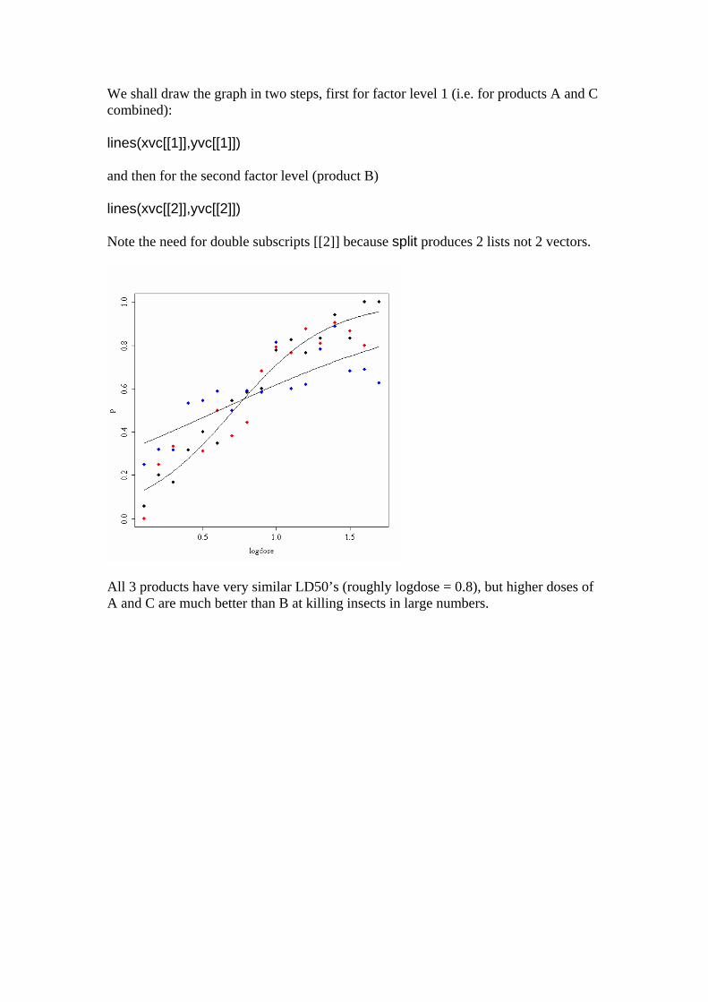
We shall draw the graph in two steps, first for factor level 1 (i.e. for products A and C combined): lines(xvc[[1]],yvc[[1]]) and then for the second factor level (product B) lines(xvc[[2]],yvc[[2]]) Note the need for double subscripts [[2]] because split produces 2 lists not 2 vectors.

All 3 products have very similar LD50’s (roughly logdose = 0.8), but higher doses of A and C are much better than B at killing insects in large numbers.

Binary Response Variables Many statistical problems involve binary response variables. For example, we often classify individuals as • dead or alive • occupied or empty • healthy or diseased • wilted or turgid • male or female • literate or illiterate • mature or immature • solvent or insolvent • employed or unemployed and it is interesting to understand the factors that are associated with an individual being in one class or the other (Cox & Snell 1989). In a study of company insolvency, for instance, the data would consist of a list of measurements made on the insolvent companies (their age, size, turnover, location, management experience, workforce training, and so on) and a similar list for the solvent companies. The question then becomes which, if any, of the explanatory variables increase the probability of an individual company being insolvent. The response variable contains only 0's or 1's; for example, 0 to represent dead individuals and 1 to represent live ones. There is a single column of numbers, in contrast to proportion data (see above). The way SPlus treats this kind of data is to assume that the 0's and 1's come from a binomial trial with sample size 1. If the probability that an animal is dead is p, then the probability of obtaining y (where y is either dead or alive, 0 or 1) is given by an abbreviated form of the binomial distribution with n = 1, known as the Bernoulli distribution:

P y p py y( ) ( ) ( )= − −1 1 The random variable y has a mean of p and a variance of p(1-p), and the object is to determine how the explanatory variables influence the value of p. The trick to using binary response variables effectively is to know when it is worth using them and when it is better to lump the successes and failures together and analyse the total counts of dead individuals, occupied patches, insolvent firms or whatever. The question you need to ask yourself is this: do I have unique values of one or more explanatory variables for each and every individual case? If the answer is ‘yes’, then analysis with a binary response variable is likely to be fruitful. If the answer is ‘no’, then there is nothing to be gained, and you should reduce your data by aggregating the counts to the resolution at which each count does have a unique set of explanatory variables. For example, suppose that all your explanatory variables were categorical (say sex (male or female), employment

(employed or unemployed) and region (urban or rural)). In this case there is nothing to be gained from analysis using a binary response variable because none of the individuals in the study have unique values of any of the explanatory variables. It might be worthwhile if you had each individual’s body weight, for example, then you could ask the question “when I control for sex and region, are heavy people more likely to be unemployed than light people? “. In the absence of unique values for any explanatory variables, there are two useful options: • analyse the data as a 2 x 2 x 2 contingency table using Poisson errors, with the

count of the total number of individuals in each of the 8 contingencies is the response variable (see Practical 11) in a data frame with just 8 rows.

• decide which of your explanatory variables is the key (perhaps you are interested

in gender differences), then express the data as proportions (the number of males and the number of females) and re-code the binary response as count of a 2-level factor. The analysis is now of proportion data (the proportion of all individuals that are female, for instance) using binomial errors (see Practical 11).

If you do have unique measurements of one or more explanatory variables for each individual, these are likely to be continuous variables (that’s what makes them unique to the individual in question). They will be things like body weight, income, medical history, distance to the nuclear reprocessing plant, and so on. This being the case, successful analyses of binary response data tend to be multiple regression analyses or complex analyses of covariance, and you should consult the relevant Practicals for details on model simplification and model criticism. In order to carry out linear modelling on a binary response variable we take the following steps: • create a vector of 0's and 1's as the response variable • use glm with family=binomial • you can change the link function from default logit to complementary log-log • fit the model in the usual way • test significance by deletion of terms from the maximal model, and compare the

change in deviance with chi-square • note that there is no such thing as overdispersion with a binary response variable,

and hence no need to change to using F tests. Choice of link function is generally made by trying both links and selecting the link that gives the lowest deviance. The logit link that we used earlier is symmetric in p and q, but the complementary log-log link is asymmetric. Death rate and reproductive effort (an ecological trade-off) We shall use a binary response variable to analyse some questions about the costs of reproduction in a perennial plant. Suppose that we have one set of measurements on plants that survived through the winter to the next growing season, and another set of measurements on otherwise similar plants that died between one growing season and the next. We are particularly interested to know whether, for a plant of a given size,

the probability of death is influenced by the number of seeds it produced during the previous year. Because the binomial denominator, n, is always equal to 1, we don’t need to specify it. Instead of binding together 2 vectors containing the numbers of successes and failures, we provide a single vector of 0’s and 1’s as the response variable. The aim of the modelling exercise is to determine which of the explanatory variables influences the probability of an individual being in one state or the other. flowering<-read.table("c:\\temp\\flowering.txt",header=T) attach(flowering) names(flowering) [1] "State" "Flowers" "Root" The first thing to get used to is how odd the plots look. Because all of the values of the response variable are just 0’s or 1’s we get to rows of points: one across the top of the plot at y = 1 and another across the bottom at y = 0. We have two explanatory variables in this example, so let’s plot the state of the plant next spring (dead or alive) as a function of its seed production this summer (Flowers) and the size of its rootstock (Root). The expectation is that plants that produce more flowers are more likely to die during the following winter, and plants with bigger roots are less likely to die than plants with smaller rootas. We use par(mfrow=c(1,2)) to get 2 plots, side-by-side: par(mfrow=c(1,2)) plot(Flowers,State) plot(Root,State)

Flowers

Sta

te

50 100 150

0.0

0.2

0.4

0.6

0.8

1.0

Root

Sta

te

0.0 0.5 1.0 1.5 2.0

0.0

0.2

0.4

0.6

0.8

1.0

It is very hard to see any pattern in plots of binary data without the fitted models. Rather few of the plants with the biggest roots died (bottom right of the right hand plot), and rather few of the plants with big seed production survived (top right of the left-hand plot). The modelling is very straightforward. It is a multiple regression with 2 continuous explanatory variables (Flowers and Root), where the response variable,

State, is binary with values either 0 or 1. We begin by fitting the full model, including an interaction term, using the * operator: model<-glm(State~Flowers*Root,binomial) summary(model) Call: glm(formula = State ~ Flowers * Root, family = binomial) Deviance Residuals: Min 1Q Median 3Q Max -1.74539 -0.44300 -0.03415 0.46455 2.69430 Coefficients: Estimate Std. Error z value Pr(>|z|) (Intercept) -2.96084 1.52124 -1.946 0.05161 . Flowers -0.07886 0.04150 -1.901 0.05736 . Root 25.15152 7.80222 3.224 0.00127 ** Flowers.Root -0.20911 0.08798 -2.377 0.01746 * (Dispersion parameter for binomial family taken to be 1) Null deviance: 78.903 on 58 degrees of freedom Residual deviance: 37.128 on 55 degrees of freedom AIC: 45.128 The first question is whether the interaction term is required in the model. It certainly looks as if it is required (p = 0.01746), but we need to check this by deletion. We use update to compute a simpler model, leaving out the interaction Flower:Root model2<-update(model , ~ . - Flowers:Root) anova(model,model2,test="Chi") Analysis of Deviance Table Model 1: State ~ Flowers * Root Model 2: State ~ Flowers + Root Resid. Df Resid. Dev Df Deviance P(>|Chi|) 1 55 37.128 2 56 54.068 -1 -16.940 3.858e-05 This is highly significant, so we conclude that the way that flowering affects survival depends upon the size of the rootstock. Inspection of the model coefficients indicates that a given level of flowering has a bigger impact on reducing survival on plants with small roots than on larger plants.

Both explanatory variables and their interaction are important, so we can not simplify the original model. Here are separate 2-D graphs for the effects of Flowers and Root on State:

Flowers

Sta

te

50 100 150

0.0

0.2

0.4

0.6

0.8

1.0

Root

Sta

te

0.0 0.5 1.0 1.5 2.0

0.0

0.2

0.4

0.6

0.8

1.0

Binary response variable with both continuous and categorical explanatory variables: Logistic Ancova parasite<-read.table("c:\\temp\\parasite.txt",header=T) attach(parasite) names(parasite) [1] "infection" "age" "weight" "sex" In this example the binary response variable is parasite infection (infected or not) and the explanatory variables are weight and age (continuous) and sex (categorical). We begin with data inspection. par(mfrow=c(1,2)) plot(infection,weight) plot(infection,age)

510

15

wei

ght

absent present

infection

050

100

150

200

age

absent present

infection

Infected individuals are substantially lighter than uninfected individuals, and occur in a much narrower range of ages. To see the relationship between infection and gender (both categorical variables) we can use table: table(infection,sex) female male absent 17 47 present 11 6 which indicates that the infection is much more prevalent in females (11/28) than in males (6/53). We begin, as usual, by fitting a maximal model with different slopes for each level of the categorical variable: model<-glm(infection~age*weight*sex,family=binomial) summary(model) Coefficients: Estimate Std. Error z value Pr(>|z|) (Intercept) -0.109124 1.375388 -0.079 0.937 age 0.024128 0.020874 1.156 0.248 weight -0.074156 0.147678 -0.502 0.616 sexmale -5.969133 4.275952 -1.396 0.163 age:weight -0.001977 0.002006 -0.985 0.325 age:sexmale 0.038086 0.041310 0.922 0.357 weight:sexmale 0.213835 0.342825 0.624 0.533 age:weight:sexmale -0.001651 0.003417 -0.483 0.629 (Dispersion parameter for binomial family taken to be 1) Null deviance: 83.234 on 80 degrees of freedom Residual deviance: 55.706 on 73 degrees of freedom AIC: 71.706

Remember that with a binary response variable, the null and residual deviance don’t mean anything, and there is no such thing as overdispersion. It certainly does not look as if any of the high order interactions are significant. Instead of using update and anova for model simplification, we can use step to compute the AIC for each term in turn: step(model) Start: AIC= 71.71 infection ~ age + weight + sex + age:weight + age:sex + weight:sex + age:weight:sex First, it tests whether the 3-way interaction is required Df Deviance AIC - age:weight:sex 1 55.943 69.943 <none> 55.706 71.706 Step: AIC= 69.94 infection ~ age + weight + sex + age:weight + age:sex + weight:sex A reduction in AIC of just 71.7 – 69.9 = 1.8 and hence not significant. Next, it looks at the 3 2-way interactions and decides which to delete first: Df Deviance AIC - weight:sex 1 56.122 68.122 - age:sex 1 57.828 69.828 <none> 55.943 69.943 - age:weight 1 58.674 70.674 Step: AIC= 68.12 infection ~ age + weight + sex + age:weight + age:sex Df Deviance AIC <none> 56.122 68.122 - age:sex 1 58.142 68.142 - age:weight 1 58.899 68.899 Call: glm(formula = infection ~ age + weight + sex + age:weight + age:sex, family = binomial) Coefficients: (Intercept) age weight sexmale age:weight age:sexmale -0.391572 0.025764 -0.036493 -3.743698 -0.002221 0.020464 Degrees of Freedom: 80 Total (i.e. Null); 75 Residual Null Deviance: 83.23 Residual Deviance: 56.12 AIC: 68.12

The step procedure suggests that we retain two 2-way interactions: age:weight and age:sex. Let’s see if we would have come to the same conclusion using update and anova. model2<-update(model,~.-age:weight:sex) anova(model,model2,test="Chi")[,-1] -age:weight:sex p = 0.626 so no evidence of 3-way interaction. Now for the 2-ways: model3<-update(model2,~.-age:weight) anova(model2,model3,test="Chi")[,-1] -age:weight p = 0.098 so no really persuasive evidence of an age:weight term model4<-update(model2,~.-age:sex) anova(model2,model4,test="Chi")[,-1] Note that we are testing all the 2-way interactions by deletion from the model that contains all 2-way interactions (model2): -age:sex p = 0.170, so nothing there, then. model5<-update(model2,~.-weight:sex) anova(model2,model5,test="Chi")[,-1] -weight:sex p = 0.672 or thereabouts. As one often finds, step has been relatively generous in leaving terms in the model. It is a good idea to try adding back marginally significant terms, to see if they have greater explanatory power when fitted on their own. model6<-update(model2,~.-weight:sex-weight:age-sex:age) model7<-update(model6,~.+weight:age) anova(model7,model6,test="Chi")[,-1] -weight:age p = 0.190. So no evidence for this interaction. Now for the main effects: model8<-update(model6,~. -weight) anova(model6,model8,test="Chi")[,-1] -weight p = 0.0003221 so weight is highly significant, as we expected from the initial boxplot: model9<-update(model6,~. -sex) anova(model6,model9,test="Chi")[,-1] -sex p = 0.020 so sex is quite significant: model10<-update(model6,~. -age) anova(model6,model10,test="Chi")[,-1]

-age p = 0.048 so age is marginally significant. Note that all the main effects were tested by deletion from the model that contained all the main effects (model6). It is worth establishing whether there is any evidence of non-linearity in the response of infection to weight or age. We might begin by fitting quadratic terms for the 2 continuous explanatory variables: model11<-glm(infection~sex+age+weight+I(age^2)+I(weight^2),family=binomial) Then dropping each of the quadratic terms in turn: model12<-glm(infection~sex+age+weight+I(age^2),family=binomial) anova(model11,model12,test="Chi")[,-1] -I(weight^2) p = 0.034 so the weight^2 term is needed. model13<-glm(infection~sex+age+weight+(weight^2),family=binomial) anova(model11,model13,test="Chi")[,-1] -I(age^2) p = 0.00990 and so is the age^2 term. It is worth looking at these non-linearities in more detail, to see if we can do better with other kinds of models (e.g. non-parametric smoothers, piece-wise linear models or step functions). An alternative approach is to use a gam rather than a glm for the continuous covariates. library(mgcv) gam1<-gam(infection~sex+s(age)+s(weight),family=binomial) plot.gam(gam1)

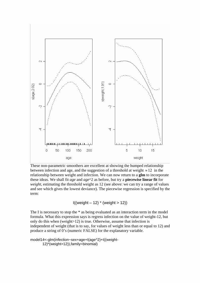
These non-parametric smoothers are excellent at showing the humped relationship between infection and age, and the suggestion of a threshold at weight 12 in the relationship between weight and infection. We can now return to a glm to incorporate these ideas. We shall fit age and age^2 as before, but try a piecewise linear fit for weight, estimating the threshold weight as 12 (see above: we can try a range of values and see which gives the lowest deviance). The piecewise regression is specified by the term:

≈

I((weight – 12) * (weight > 12))

The I is necessary to stop the * as being evaluated as an interaction term in the model formula. What this expression says is regress infection on the value of weight-12, but only do this when (weight>12) is true. Otherwise, assume that infection is independent of weight (that is to say, for values of weight less than or equal to 12) and produce a string of 0’s (numeric FALSE) for the explanatory variable. model14<-glm(infection~sex+age+I(age^2)+I((weight-

12)*(weight>12)),family=binomial)

The effect of sex on infection is not quite significant (p = 0.07 for a chi square test on deletion), so we leave it out: model15<-update(model14,~.-sex) anova(model14,model15,test="Chi") Analysis of Deviance Table Resid. Df Resid. Dev Df Deviance P(>|Chi|) 1 76 48.687 2 77 51.953 -1 -3.266 0.071 summary(model15) Coefficients: Estimate Std. Error z value Pr(>|z|) (Intercept) -3.1207575 1.2663090 -2.464 0.01372 * age 0.0765785 0.0323274 2.369 0.01784 * I(age^2) -0.0003843 0.0001845 -2.082 0.03732 * I((weight - 12) * (weight > 12)) -1.3511514 0.5112930 -2.643 0.00823 ** (Dispersion parameter for binomial family taken to be 1) Null deviance: 83.234 on 80 degrees of freedom Residual deviance: 51.953 on 77 degrees of freedom AIC: 59.953 This is our minimal adequate model. All the terms are significant when tested by deletion, the model is parsimonious, and the residuals are well behaved. A 3x3 crossover trial In a crossover experiment, the same set of treatments is applied to different individuals (or locations) but in different sequences to control for order effects. So a set of farms might have predator control for 3 years followed by no control for 3 years, while another set may have three years of no control followed by 3 years of predator control. Crossover trials are most commonly used on human subjects, as in the present example of a drug trial on a new pain killer using a group of headache sufferers. There were 3 experimental treatments: a control pill that had no pain killer in it (the ‘placebo’), neurofen, and brandA, the new product to be compared with the established standard. The interesting thing about crossover trials is that they involve repeated measures on the same individual, so a number of important questions need to be addressed: 1) does the order in which the treatments are administered to subjects matter? 2) if so, are there any carryover effects from treatments administered early on ? 3) are there any time series trends through the trial as a whole?

The response variable, y, is binary: 1 means pain relief was reported and 0 means no pain relief. rm(y) crossover<-read.table("c:\\temp\\crossover.txt",header=T) attach(crossover) names(crossover) [1] "y" "drug" "order" "time" "n" "patient" “carryover" In a case like this, data inspection is best carried out by summarising the totals of the response variable over the explanatory variables. Your first reaction might be to use table to do this, but this just counts the number of cases table(drug) A B C 86 86 86 which shows only that all 86 patients were given each of the 3 drugs: A is the placebo, B neurofen and C BrandA. What we want is the sum of the y values (the number of cases of expressed pain relief) for each of the drugs. The tool for this is tapply: the order of its 3 arguments are tapply(response variable, explanatory variable(s), action) so we want tapply(y,drug,sum) A B C 22 61 69 Before we do any complicated modelling, it is sensible to see if there are any significant differences between these 3 counts. It looks (as we hope that it would) as if pain relief is reported less frequently (22 times) for the placebo than for the pain killers (61 and 69 reports respectively). It is much less clear, however, whether BrandA (69) is significantly better than neurofen (61). Looking on the bright side, there is absolutely no evidence that it is significantly worse than neurofen ! To do a really quick chi square test on these three counts we just type: glm(c(22,61,69)~1,family=poisson) and we see Degrees of Freedom: 2 Total (i.e. Null); 2 Residual Null Deviance: 28.56 Residual Deviance: 28.56 AIC: 47.52 which is a chi square of 28.56 on just 2 degrees of freedom, and hence highly significant. Now we look to see whether there are any obvious effects of treatment sequence on reports of pain relief. In a 3-level crossover like this there are 6 orders: ABC, ACB, BAC, BCA, CAB and CBA. Patients are allocated to order at random.

There were different numbers of replications in this trial, which we can see using table on order and drug: table(drug,order) 1 2 3 4 5 6 A 15 16 15 12 15 13 B 15 16 15 12 15 13 C 15 16 15 12 15 13 which shows that replication varied from a low of 12 patients for order 4 (BCA) to a high of 16 for order 2 (ACB). A simple way to get a feel for whether or not order matters is to tabulate the total reports of relief by order and by drug: tapply(y,list(drug,order),sum) 1 2 3 4 5 6 A 2 5 5 2 4 4 B 13 13 10 10 10 5 C 12 13 13 10 9 12 Nothing obvious here. C (our new drug) did worst in order 5 (CAB) when it was administered first (9 cases), but this could easily be due to chance. We shall see. It is time to begin the modelling. order<-factor(order) With a binary response, we can make the single vector of 0’s and 1’s into the response variable directly, so we type: model<-glm(y~drug*order+time,family=binomial) There are lots of different ways of modelling an experiment like this. Here we are concentrating on the treatment effects and worrying less about the correlation and time series structure of the repeated measurements. We fit the main effects of drug (a 3-level factor) and order of administration (a 6-level factor) and their interaction (which has 2 x 5 = 10 d.f.). We also fit time to see if there is any pattern to the reporting of pain relief through the course of the experiment as a whole. This is what we find: summary(model) Call: glm(formula = y ~ drug * order + time, family = binomial) Deviance Residuals: Min 1Q Median 3Q Max -2.2642 -0.8576 0.5350 0.6680 2.0074 Coefficients: Estimate Std. Error z value Pr(>|z|) (Intercept) -1.862803 1.006118 -1.851 0.064101 .

drugB 3.752595 1.006118 3.730 0.000192 *** drugC 3.276086 0.771058 4.249 2.15e-005 *** order2 1.083344 0.930765 1.164 0.244453 order3 1.187650 0.858054 1.384 0.166322 order4 0.280355 1.092937 0.257 0.797553 order5 0.869198 0.881368 0.986 0.324038 order6 1.078864 0.771058 1.399 0.161753 time -0.008997 0.385529 -0.023 0.981383 drugB.order2 -1.479810 1.512818 -0.978 0.327985 drugC.order2 -1.012297 1.159837 -0.873 0.382776 drugB.order3 -2.375300 1.330330 -1.785 0.074181 . drugC.order3 -0.702144 1.232941 -0.569 0.569026 drugB.order4 -0.551713 1.680933 -0.328 0.742747 drugC.order4 -0.066207 1.428863 -0.046 0.963043 drugB.order5 -2.038855 1.338492 -1.523 0.127697 drugC.order5 -1.868020 1.208188 -1.546 0.122072 drugB.order6 -3.420667 1.222788 -2.797 0.005151 ** (Dispersion parameter for binomial family taken to be 1) Null deviance: 349.42 on 257 degrees of freedom Residual deviance: 268.85 on 240 degrees of freedom AIC: 304.85 Remember that with binary response data we are not concerned with overdispersion. Looking up the list of coefficients, starting with the highest order interactions, it looks as if drugB.order6 with its t value of 2.768 is significant, and drugB.order3, perhaps. We test this by deleting the drug:order interaction from the model model2<-update(model,~. - drug:order) anova(model,model2,test="Chi") Analysis of Deviance Table Model 1: y ~ drug * order + time Model 2: y ~ drug + order + time Resid. Df Resid. Dev Df Deviance P(>|Chi|) 1 240 268.849 2 249 283.349 -9 -14.499 0.106 There is no compelling reason to retain this interaction (p > 10%). So we leave it out and test for an effect of time: model3<-update(model2,~. - time) anova(model2,model3,test="Chi") Analysis of Deviance Table Model 1: y ~ drug + order + time Model 2: y ~ drug + order

Resid. Df Resid. Dev Df Deviance P(>|Chi|) 1 249 283.349 2 250 283.756 -1 -0.407 0.523 Nothing at all. What about the effect of order of administration of the drugs? model4<-update(model3,~. - order) anova(model3,model4,test="Chi") Analysis of Deviance Table Model 1: y ~ drug + order Model 2: y ~ drug Resid. Df Resid. Dev Df Deviance P(>|Chi|) 1 250 283.756 2 255 286.994 -5 -3.238 0.663 Nothing. What about the differences between the drugs? summary(model4) Coefficients: Estimate Std. Error z value Pr(>|z|) (Intercept) -1.0678 0.2469 -4.325 1.53e-05 *** drugB 1.9598 0.3425 5.723 1.05e-08 *** drugC 2.4687 0.3664 6.739 1.60e-11 *** (Dispersion parameter for binomial family taken to be 1) Null deviance: 349.42 on 257 degrees of freedom Residual deviance: 286.99 on 255 degrees of freedom AIC: 292.99 Notice that, helpfully, the names of the treatments appear in the coefficients list . Now it is clear that our drug C had log odds greater than neurofen by 2.4687 – 1.9598 = 0.5089 . The standard error of the difference between two treatments is about 0.366 (taking the larger (less well replicated) of the two values) so a t test between neurofen and our drug gives t = 0.5089/0.366 = 1.39. This is not significant. The coefficients are now simply the logits of our original proportions that we tabulated during data exploration: 22/86, 61/86 and 69/86 (you might like to check this). The analysis tells us that 69/86 is not significantly greater than 61/86. If we had known to begin with that none of the interactions, sequence effects or temporal effects had been significant, we could have analysed these results much more simply, like this relief<-c(22,61,69) patients<-c(86,86,86) treat<-factor(c("A","B","C"))

model<-glm(cbind(relief,patients-relief)~treat,binomial) summary(model) Coefficients: Estimate Std. Error z value Pr(>|z|) (Intercept) -1.0678 0.2471 -4.321 1.55e-005 *** treatB 1.9598 0.3427 5.718 1.08e-008 *** treatC 2.4687 0.3666 6.734 1.65e-011 *** (Dispersion parameter for binomial family taken to be 1) Null deviance: 6.2424e+001 on 2 degrees of freedom Residual deviance: 1.5479e-014 on 0 degrees of freedom AIC: 19.824 Treatments B and C differ by only about 0.5 with a standard error of 0.367, so we may be able to combine them. Note the use of != for “not equal to” t2<-factor(1+(treat != "A")) model2<-glm(cbind(relief,patients-relief)~t2,binomial) anova(model,model2,test="Chi") Analysis of Deviance Table Model 1: cbind(relief, patients - relief) ~ treat Model 2: cbind(relief, patients - relief) ~ t2 Resid. Df Resid. Dev Df Deviance P(>|Chi|) 1 0 6.376e-15 2 1 2.02578 -1 -2.02578 0.15465 We can reasonably combine these two factor levels, so the minimum adequate model as only 2 parameters, and we conclude that the new drug is not significantly better than neurofen. But if they cost the same, which of them would you take if you had a headache?