
LearnCAx Blog 3482 Electrostatic Precipitators Esp Analysis Using Cfd

ALMA MATER STUDIORUM - UNIVERSITÀ DI BOLOGNAPhD COURSE: INFORMATION TECHNOLOGYXXIII CYCLE - SCIENTIFIC DISCIPLINARY SECTOR ING-INF/01
Statistical Methods for
Analysis and Processing of
Medical Ultrasound
Applications to Segmentation and Restoration
Martino Alessandrini
SUPERVISORProf. Guido Masetti
COORDINATORProf. Claudio Fiegna
ARCES - ADVANCED RESEARCH CENTER ON ELECTRONIC SYSTEMSJANUARY 2008 - DECEMBER 2010


Martino Alessandrini: Statistical methods for analysis andprocessing of medical ultrasound: applications to segmentationand restoration. Dissertation for the degree of Doctor ofPhilosophy in Information Technology, March 2011.


Contents
Contents i
Abstract v
Sommario vii
Introduction ix
I Background on Medical Ultrasound 1
1 Ultrasound imaging systems 5
1.1 Overview . . . . . . . . . . . . . . . . . . . . . . . 51.2 Ultrasound system architecture . . . . . . . . . . 91.3 Conclusion . . . . . . . . . . . . . . . . . . . . . . 11
2 Deterministic description of ultrasound 13
2.1 Wave equation . . . . . . . . . . . . . . . . . . . . 142.2 Scattered eld . . . . . . . . . . . . . . . . . . . . 142.3 Incident eld . . . . . . . . . . . . . . . . . . . . . 152.4 RF echo signal . . . . . . . . . . . . . . . . . . . . 172.5 Point Spread Function . . . . . . . . . . . . . . . . 192.6 Conclusion . . . . . . . . . . . . . . . . . . . . . . 21
3 Statistical description of ultrasound 23
3.1 Rayleigh distribution . . . . . . . . . . . . . . . . 243.2 Nakagami distribution . . . . . . . . . . . . . . . 263.3 Generalized gaussian distribution . . . . . . . . . 273.4 Comparison . . . . . . . . . . . . . . . . . . . . . 293.5 Conclusion . . . . . . . . . . . . . . . . . . . . . . 30
i
ii Contents
II Restoration of Ultrasound Images 33
4 Deconvolution problem 37
4.1 Problem statement . . . . . . . . . . . . . . . . . . 384.2 Predictive deconvolution . . . . . . . . . . . . . . 394.3 Maximum a posteriori deconvolution . . . . . . . 454.4 PSF estimation . . . . . . . . . . . . . . . . . . . . 534.5 Conclusion . . . . . . . . . . . . . . . . . . . . . . 56
5 Deconvolution and tissue characterization 57
5.1 Reectivity model and optimization scheme . . . 615.2 Materials and methods . . . . . . . . . . . . . . . 665.3 Results . . . . . . . . . . . . . . . . . . . . . . . . . 705.4 Conclusion . . . . . . . . . . . . . . . . . . . . . . 77
III Segmentation in Echocardiography 79
6 Level-set segmentation 85
6.1 General . . . . . . . . . . . . . . . . . . . . . . . . 856.2 Region based level-sets . . . . . . . . . . . . . . . 876.3 Localized level sets . . . . . . . . . . . . . . . . . . 896.4 Statistical level sets . . . . . . . . . . . . . . . . . . 926.5 Shape prior constraints . . . . . . . . . . . . . . . 936.6 Conclusion . . . . . . . . . . . . . . . . . . . . . . 95
7 Myocardium anatomy and functioning 97
7.1 Heart anatomy . . . . . . . . . . . . . . . . . . . . 977.2 Heart functioning . . . . . . . . . . . . . . . . . . 997.3 Le ventricle . . . . . . . . . . . . . . . . . . . . . 997.4 Le ventricle segmentation . . . . . . . . . . . . . 1017.5 Conclusion . . . . . . . . . . . . . . . . . . . . . . 103
8 Myocardium segmentation 105
8.1 Proposed segmentation framework . . . . . . . . 1058.2 Implementation issues . . . . . . . . . . . . . . . 1178.3 Materials and methods . . . . . . . . . . . . . . . 1188.4 Performance metrics . . . . . . . . . . . . . . . . 1188.5 Results . . . . . . . . . . . . . . . . . . . . . . . . . 1198.6 Beyond ultrasound . . . . . . . . . . . . . . . . . 1228.7 Conclusion . . . . . . . . . . . . . . . . . . . . . . 126
9 Conclusion 129

Contents iii
A Derivation of the Bhattacharyya level-set function 131
B Computation of spatially-variant blurring operators 133
B.1 Spatially invariant PSF . . . . . . . . . . . . . . . 133B.2 Spatially variant PSF . . . . . . . . . . . . . . . . . 135B.3 Preconditioning of spatially variant kernels . . . 137
C Complex Generalized Gaussian Distribution 139
D Chen algorithm 141
Publications list 143
Bilbiography 147

Abstract
Medical ultrasound is nowadays commonlyemployed in the clinical practice for assessing possi-ble abnormalities in several parts of the human body.
Due to the simple image formation process, ultrasound systemsare reduced size reasonably priced machines, easily aordableeven for small low budget ambulatories widespread distributedon the territory. Besides that ultrasound is a non ionizing radi-ation and practically harmless to the patient. Despite these de-sirable features, ultrasound scans have a considerably low imagequality as compared to that of other popular techniques as X-ray,Magnetic Resonance Imaging and Computed Tomography, and,as a consequence, their interpretation is oen subjective and un-clear, and their diagnostic reliability low. In this context, the de-velopment of soware tools providing the physician with assis-tance in the image reading and analysis process is a continuouschallenge for many researchers working in the eld.
Due to the noisy nature of ultrasound frames, successful tech-niques cannot be directly borrowed from the densely populatedliterature on the processing of natural images, but rather tailoredto the ultrasound very peculiar nature. In particular, applica-tions relying on speckle noise statistics as the driving criterionhave led to eective solutions for a wide range of problems.
In this thesis two major topics encountered in medical ul-trasound are addressed i.e. the problems of image restorationand segmentation. For both, original author contributions willbe discussed and their performance compared to the state of theart. In the former case, a novel deconvolution technique will bepresented, expressively designed for an improved tissue charac-terization. Phantom studies will show a relevant increase in clas-sication accuracy, along with the superiority of the proposedalgorithm over standard ones. e problem of myocardium de-tection from 2D echocardiography will be then considered and
v

vi Abstract
an original active contour based solution proposed. e result-ing algorithm will be validated on a set of clinical ultrasoundsequences. Results will show the proposed method on realisticclinical data to be feasible and accurate.
Sommario
Esami ecografici sono comunemente prescritti nella prat-ica clinica per la diagnosi di possibili patologie di di-versi organi del corpo umano. La semplicità del pro-
cesso di formazione dell’immagine fa sì che le apparecchiatureecograche siano macchinari di dimensioni relativamente pic-cole e a basso costo, facilmente annoverabili nel parcomacchinedi piccoli ambulatori a basso budget capillarmente distribuitinel territorio. A ciò si aggiunga che l’ecograa è innocua peril paziente, essendo gli ultrasuoni onde non ionizzanti. Mal-grado questi vantaggi, le immagini ecograche hanno una qual-ità considerevolmente inferiore rispetto a quella ottenuta conaltre tecniche di imaging, quali raggi X, risonanza magneticae tomograa computerizzata, il che ne rende la lettura spessosoggettiva e non chiara, e la validità diagnostica assai limitata. Inquest’ottica la comunità scientica ha proposto numerosi so-ware per supportare il medico nella lettura e l’analisi delle im-magini ecograche.
Sfortunatamente, l’elevata rumorosità delle immagini eco pre-clude l’adozione di algoritmi proposti per l’elaborazione di im-magini naturali, sui quali esiste un’ampia letteratura, e imponeinvece lo sviluppo di tecniche ad hoc. In particolare, le appli-cazioni più ecaci si basano sull’utilizzo della distribuzione sta-tistica del rumore. In questo contesto si inserisce il presentemanoscritto, nel quale vengono arontano due problematicherelative all’elaborazione di immagini ecograche, nella fattispeciela loro deconvoluzione e segmentazione. Per entrambe verrannodescritte soluzioni originali proposte dall’autore, le prestazionidelle quali saranno confrontate con lo stato dell’arte.
Nel primo caso, verrà descritta una nuova tecnica di decon-voluzione in grado di migliorare la caratterizzazione di tessutitramite ultrasuoni. Da risultati ottenuti su fantoccio verràmessoin luce come l’algoritmo proposto sia in grado di determinare
vii

viii Sommario
una riduzione sostanziale dell’errore di classicazione e insiemesuperare le performance ottenute tramite tecniche standard.
Verrà quindi presentato un nuovo algoritmo per la segmen-tazione del miocardio da immagini eco bidimensionali, basatosulla tecnica dei contorni attivi. Una valutazione dell’algoritmosu sequenze ecocardiograche rivelerà le sue potenzialità comestrumento utile di supporto in ambito clinico.

Introduction
Since the early 1950s, ultrasound use in medicine has beenthe basis for several procedures that are widespread in to-day’s clinical practice. e principal application is in the
eld of medical imaging. Medical ultrasound imaging relies onthe same principles as sonar or radar units: the ultrasound probeproduces a (pulsed) acoustic pressure eld; the eld propagatesthrough the tissue and is partially reected and scattered due tothe inherent inhomogeneity of most tissues. e backscatteredsignal is received by the same probe and converted into a grayscale image of the organ.
Medical ultrasound has several advantages over other popu-lar imaging modalities as Magnetic Resonance Imaging (MRI),X-ray and Computed Tomography (CT). At rst, unlike X-rayand CT, ultrasound is a non ionizing radiation and hence prac-tically harmless to the human body. Moreover, the simple phe-nomena involved in the signal generation and acquisition pro-cess along with the little computation needed for the image cre-ation (fundamentally an amplitude to gray scale conversion), al-low ultrasound systems to work at extremely high frame rates,easily of the order of 100 frames/sec. is makes ultrasound thestandard tool for diagnosis of disease based on organs dynam-ics, as it is in echocardiography. Further advantages connectedwith ultrasound systems are the their cost eectiveness and re-duced size, making their availability possible even in small locallow budget ambulatories. is is instead not the case for X-ray,CT andMRI, whose installation, besides relevant costs, requiresextendeddedicated areas. In Figure 1 a standard ultrasound ima-ging system is illustrated.
Unfortunately, all these advantages come at a price. i.e. thereduced image quality as compared to that of X-ray, CT orMRI.is is principally due to the low spatial resolution, directly con-nected with the nite bandwidth of the transducer and the non-
ix

x Introduction
Figure 1: External parts of an ultrasound imaging system. Imagefrom [1, pp. 298].
negligible width of the acoustic beam, along with the character-istic granular texture referred as speckle noise. All these factorsmake sometimes the interpretation of ultrasound frames highlyambiguous and subjective, even for expert physicians, therebylimiting their diagnostic reliability. In Figure 2 a short axis sliceof the le ventricle is represented from 2D echocariography andcardiacMRI: it is evident how image reading is fairly less straight-forward in the ultrasound case.
Improving the quality and diagnostic reliability of medicalultrasound has always represented a continuous challenge formany scientists working in the eld. e eorts aremainly spentin two directions: on one side improving the acquisition mod-ality itself, by designing new transducers, more sophisticatedbeam-forming, compounding or apodization schemes; on theother, acting on the acquired image at a post processing stepwithsuitable signal and image processing tools. In particular, in thisthesis the second approach is considered.
Unfortunately, the noisy nature of ultrasound imagesdegrades the performance of standard algorithms developed fornatural scenes and implies the design of ad hoc techniques. eyusually rely on considering the speckle not as a noise term to beeliminated, but rather as a precious source of information. It isindeed well established that speckle distribution is strictly cor-related with the micro-structure of the underlying tissue. is

xi
(a) (b)
Figure 2: Short axis view of the le ventricle from 2Dechocardiography (a) and cardiac MRI (b).
principle is exploited in awide range of applications as classica-tion, segmentation, deconvolution and tracking, to make someexamples. In this context, this manuscript addresses two majorproblems encountered in medical ultrasound, both tackled withstatistically inspired approaches: the problem of image decon-volution and segmentation.
Deconvolution in medical imaging is commonly employedin the purpose of a visual quality improvement, so to provide thephysician with better contrasted and resolved data, suitable foreasier interpretation. is is done by removing to the maximumextent possible the blurring eect associated with the non-idealPoint Spread Function of the ultrasound system and restoring anestimate of the tissue response, also called reectivity. is prob-lem has been diusively addressed in literature, the most suc-cessful solutions being based on Wiener ltering and l 1-normoptimization.
Conversely, this manuscript describes a conceptually novelapplication of deconvolution: from the observation that the re-ectivity of a tissue carries cleaner information on its structurethan the raw echo signal does, the possibility of exploiting de-convolutionnotmerely as an image enhancement tool, but ratheras a pre-processing step for easing ultrasonic tissue characteriza-tion is investigated. In this perspective, standard deconvolutionalgorithms reveal strong limitations, principally ascribed to thesimplied tissue models they make use of. Indeed, though theseare sucient for producing appreciable image quality improve-
xii Introduction
ment, they otherwise induce a statistical bias in the statistics ofthe restored reectivity, making it unusable for characterizationpurposes.
Hereto, a novel deconvolution method for ultrasound im-ages has been developed and will be described in this thesis.e algorithm is derived on the base of a non-standard statisticalmodel for the tissue response, dened by the Generalized Gaus-sian Distribution. By means of two distinct parameters, calledscale and shape parameter, this distribution allows sequences ofarbitrary energy and sparsity to be generated, and is thereforeadequate for providing an accurate description to the most gen-eral tissue structures. Deconvolution is then tackled as a maxi-mum a posteriori estimate, in which tissue reectivity is restoredalongwith an estimate of the associated scale and shape parame-ter. An ExpectationMaximization framework is designed to ad-dress this task. An evaluation of performance will be presentedon experimental data from several tissue-mimicking phantomshaving a well-dened particle concentration. ese studies willshow improvements in classication accuracy of up to the 20%and the superiority of the proposed algorithmover standard ones.
e second problem considered is myocardium segmenta-tion from 2D echocardiography. Echocardiography is one of theleading applications of ultrasound in medicine, indeed this isthe standard technique to examine myocardial function in pa-tients with known or suspected heart disease. In clinical prac-tice, the analysis mainly relies on visual inspection and manualsegmentation by experienced cardiologists. is approach, be-sides being tedious and time consuming, suers from a subjec-tive bias, due to the inherent low signal-to-noise ratio (SNR) ofultrasound scans. An automated procedure is therefore desir-able both to reduce intra- and inter-observer variability in bor-der detection and to speed up the segmentation process.
While great attention has been given to the segmentation ofthe endocardium (the innermost layer of tissue surrounding theventricular cavity), very limited literature addresses the detec-tion of the epicardium (the outer layer). is is due to the factthat signal dropouts and complex interactions between the ul-trasonic pulse and the tissue make the epicardial contour ap-pear highly heterogeneous and discontinuous. Nevertheless, atrustful detection of both structures would have a high clinicalrelevance, as it wouldmake the computation of fundamental pa-rameters possible.
Hereto, an original segmentation algorithm based on level

xiii
sets, specically designed for the detection of the wholemyocar-dium, has been developed and is described in this thesis. esegmentation ow proceeds by seeking the maximum statisti-cal separation between target, i.e. the myocardium, and back-ground. In order to deal with low-contrast or missing bound-aries, a localized version of standard region-based methods isadopted. Moreover, shape prior information is eciently em-bedded in the evolution equation, forcing the active contour tobe approximately annular. is prevents the detection of unde-sired small structures, like papillary muscles. With the resultingformalism the detection of both endo- and epicardium is ad-dressed eciently with a single level-set function. A validationwill be presented from a set of 59 images acquired from 5 pa-tients. ese results will show that the proposed method on re-alistic clinical data is feasible and accurate.
] ] ]
e manuscript is organized as follows. Some backgroundmaterial will be presented in Part I. Ultrasound imaging systemswill be briey described in Chapter 1 and their main featuresexamined. e focus will then move to the description of theultrasound echo signal. In particular modeling the echo acqui-sition as a linear time variant system will be discussed in Chap-ter 2, which will be essential in the formulation of the restor-ation problem. Statistical inspired algorithms typically rely onmodeling the ultrasound echo amplitude by means of paramet-ric probability density functions. Hereto, some popular modelswill be reviewed in Chapter 3. ey will be exploited both inimage restoration and segmentation.
eproblemof image restorationwill be addressed inPart II.e problem will be formulated in Chapter 4 where most com-mon solutions, as Wiener lter and l 1-norm optimization, willbe presented as well. e original restoration scheme will be -nally derived and evaluated in Chapter 5.
Myocardium segmentation will be discussed in Part III. InChapter 6 all the theoretical elements needed for a full under-standing of the algorithm will be given. en Chapter 7 will il-lustrate the main aspects of heart morphology and functioningand address the clinical validity of the segmentation phase. eproposed segmentation framework will be nally presented andevaluated in Chapter 8.


I - Background on Medical Ultrasound


Summary
Ultrasound, because of its ecacy, low cost, real-timecapability and safety, is oen the preferredmedical ima-ging modality and nds a number of applications for
dierent parts of the human body. In obstetrics it is commonlyemployed for 2D or, more recently, 3D in vivo imaging of the fe-tus. Female (usually) breast ultrasound is primarily used for de-termining the nature of breast abnormality or as a breast cancerscreening test supplemental to mammography. Cardiac ultra-sound is employed for early diagnosis and of heart disease andprevention of stroke. Vascular and cardiovascular ultrasound isused for monitoring blood ux through veins and arteries. Be-sides, the possibility of real time visualization is exploited in ul-trasound guided biopsy and catheter placement. As an exampleof ultrasound diusion, 5 millions exams were estimated to begiven weekly worldwide in 2000 [1]. Figure A illustrates the in-cidence of ultrasound on the overall medical imaging exams.
When compared to other imaging modalities, ultrasoundpresents several advantages and shortcomings. ese aspectswill be examined in Chapter 1, where main features of ultra-sound systems will be reviewed and put in relation with thoseof alternative available techniques. e principal limitation as-sociated to ultrasound imaging is a reduced image quality. Inorder to compensate this lack of image information many com-puter tools have been and are currently presented to the scien-tic community. ese algorithms commonly rely on models ofthe acquisition process as well as of the image content. In thiscontext, in Chapter 2 a time-variant linear model of the imageformation process will be derived. It will be obtained from de-terministically solving the acoustic waves equation for the caseof so tissues. Conversely, in Chapter 3 several parametric sta-tistical models of the echo signal amplitude distribution will bereviewed.
3

4 Introduction
Figure A: Estimated number of imaging exams in 2000. Imagefrom [1, pp. 22].
Chapter 1Ultrasound imaging systems
In this chapter general aspects of medical ultrasound ima-ging are reviewed. In §1.1 an overview is presented on themain properties of ultrasound imaging systems, with an at-
tention to resolution, penetration and safety. In §1.2 the archi-tecture of an ultrasound imaging system in explained through asimplied block diagram. In §1.3 some concluding remarks areaddressed.
1.1 Overview
epresent clinical ultrasound scanners process signals in aman-ner similar to that of sonar or radar units. To interrogate a tissue,the ultrasound probe produces a (pulsed) acoustic pressure eld.e eld propagates through the tissue and is partially reectedand scattered due to the inherent inhomogeneity ofmost tissues.e backscattered signal is received usually by the same probe,supplying useful information about the locations of tissue inho-mogeneities and their relative strengths.
Echo amplitude is proportional to the reection coecientof those tissue-tissue interfaces encountered along the propa-gation path. Values of the reection coecient for some com-mon interfaces encountered in the medical eld are reportedin Table 1.1. A high reection coecient halts the pulse prop-agation and makes underneath structures invisible. is factmakes ultrasound unusable in certain situations, e.g. it is notan ideal imaging technique for the bowel or organs obscured bythe bowel (CT scanning and MRI are the methods of choice inthis setting); for the same reason ultrasound can only see the
5

6 Ultrasound imaging systems
Interface Reflection [0,1]
so tissue - air 0.99
so tissue - lung 0.52
so tissue - bone 0.43
vitreous humor - eye lens 0.01
fat - liver 0.79
so tissue - fat 0.0069
so tissue - muscle 0.0004
water - lucote 0.13
oil - so tissue 0.0043
Table 1.1: Reection coecient for common interfaces [2].
outer surface of bony structures and not what lies within (MRIis typically preferred here). In cardiac ultrasound, the major ap-plication of ultrasound in medicine, the physician is expectedobtain clean views of the heart by suitably orientating the trans-ducer through the small acoustic windows oered by the rib cage.A big expertise is requested here because of the number of ac-cess windows, the dierences in anatomy, and themany possibleplanes of view. Experience is required besides to nd relevantplanes and targets of diagnostic signicance and to optimize in-strumentation, as well as to recognize, interpret, and measureimages for diagnosis. Such an operation dependency is a rstlimitation of medical ultrasound.
1.1.1 Resolution
Axial spatial resolution of ultrasound systems is typically chosenequal to 2 wavelength:
λax(mm) = 2c
fc(1.1)
where fc is the transducer center frequency and c is the soundvelocity. Sound speed is highly medium dependent, cf. Table 1.2and [3]. A mean value commonly agreed for so tissues is cav= 1540 m/s. For typical frequencies in use ranging from 1 to 15MHz axial resolution roughly varies from 0.3 to 3 mm. Con-versely, lateral spatial resolution is highly depth variant princi-pally due to the beamforming. In particular, this resolution isbest at the focal length distance and widens away from this dis-tance in a nonuniform way because of diraction eects caused

1.1. Overview 7
Interface sound velocity (m/s) Density (Kg/m3)
Muscles 1580 1070
Liver 1550 1060
Fat 1459 920
Brain 1560 1028
Kidney 1560 1040
Spleen 1570 1059
Blood 1575 1060
Bones 4080 1620
Eye 1670 1135
Lungs 650 430
Table 1.2: Speed of sound and acoustic impedance in somecommon tissues.
Figure 1.1: Spatial resolution of the acoustic pulse in the lateral andelevation dimensions. Acoustic pressure amplitude contours are -6
dB relative to the peak amplitude within each slice of thepoint-spread function (PSF) as it propagates. Image from [4, pp. 6]
by apertures on the order of a few to tens of wavelengths. isfact is illustrated in Figure 1.1.
Another factor in determining resolution is attenuation. At-tenuation steals energy from the ultrasound eld as it propagatesand eectively lowers the center frequency of the remaining sig-nals. From (1.1) this implies that axial resolution decreases withthe distance from the emitting aperture.
Finally, ultrasound image quality is highly degraded by thepresence of granular texture patterns normally referred as specklenoise. Speckle is generated by the constructive and destructive
8 Ultrasound imaging systems
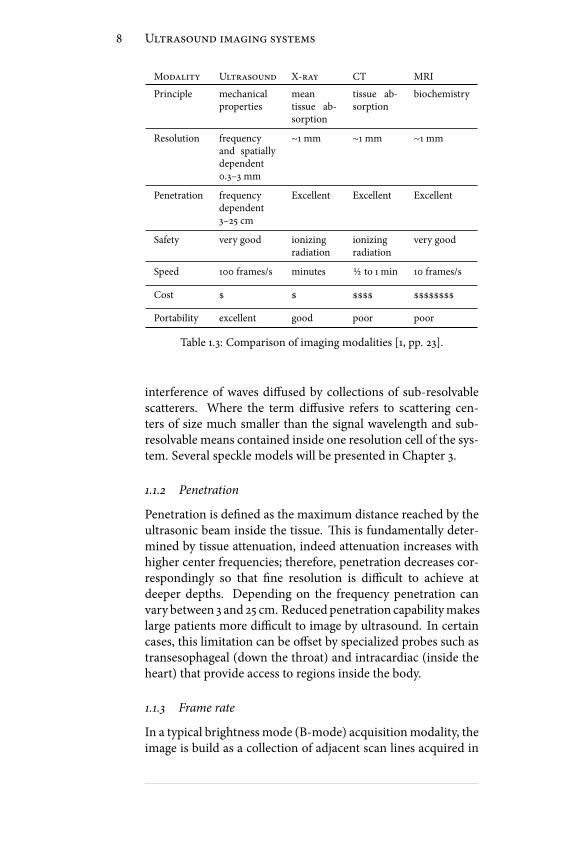
Modality Ultrasound X-ray CT MRI
Principle mechanicalproperties
meantissue ab-sorption
tissue ab-sorption
biochemistry
Resolution frequencyand spatiallydependent0.3–3 mm
∼1 mm ∼1 mm ∼1 mm
Penetration frequencydependent3–25 cm
Excellent Excellent Excellent
Safety very good ionizingradiation
ionizingradiation
very good
Speed 100 frames/s minutes 1⁄2 to 1 min 10 frames/s
Cost $ $ $$$$ $$$$$$$$
Portability excellent good poor poor
Table 1.3: Comparison of imaging modalities [1, pp. 23].
interference of waves diused by collections of sub-resolvablescatterers. Where the term diusive refers to scattering cen-ters of size much smaller than the signal wavelength and sub-resolvable means contained inside one resolution cell of the sys-tem. Several speckle models will be presented in Chapter 3.
1.1.2 Penetration
Penetration is dened as the maximum distance reached by theultrasonic beam inside the tissue. is is fundamentally deter-mined by tissue attenuation, indeed attenuation increases withhigher center frequencies; therefore, penetration decreases cor-respondingly so that ne resolution is dicult to achieve atdeeper depths. Depending on the frequency penetration canvary between 3 and 25 cm. Reducedpenetration capabilitymakeslarge patients more dicult to image by ultrasound. In certaincases, this limitation can be oset by specialized probes such astransesophageal (down the throat) and intracardiac (inside theheart) that provide access to regions inside the body.
1.1.3 Frame rate
In a typical brightnessmode (B-mode) acquisitionmodality, theimage is build as a collection of adjacent scan lines acquired in

1.2. Ultrasound system architecture 9
Figure 1.2: Block diagram of an ultrasound imaging system.
sequence. Assuming a number N of scan lines, a maximumdepth D and a sound speed c, the frame rate FR is:
RF = c
2DN(1.2)
For an image 15 cm deep and 50 scan lines the frame rate is ap-proximately 100 frames/sec, i.e. a real time visualization of theorgan is allowed.
1.1.4 Safety
As acoustic waves are employed, diagnostic ultrasound does nothave any cumulative side eects. For very particular ultrasoundapplications as hyperthermia, lithotripsy or HIFU, high powerregime is involved which is proved to induce bioeects. Nev-ertheless these cases will not be discussed here. e interestedreader is otherwise addressed to [1, chap. 15]. Besides, diagnos-tic ultrasound is also generally non invasive, excluding of course“trans” and “intra” families of transducers.
All the features reviewed in this section are compared to theone of other popular medical imaging modalities in Table 1.3.
1.2 Ultrasound system architecture
In this section B-mode imaging will be considered only. Othermodes exists, as A-mode and M-mode, sometimes employed inthe diagnostic practice, for which the reader is addressed to [1,
10 Ultrasound imaging systems
Figure 1.3: Conceptual diagram of phased array beamforming.
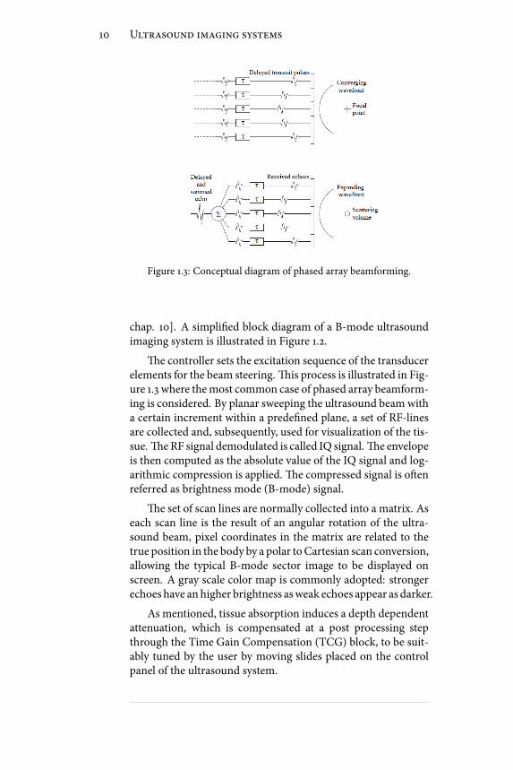
chap. 10]. A simplied block diagram of a B-mode ultrasoundimaging system is illustrated in Figure 1.2.
e controller sets the excitation sequence of the transducerelements for the beam steering. is process is illustrated in Fig-ure 1.3 where themost common case of phased array beamform-ing is considered. By planar sweeping the ultrasound beamwitha certain increment within a predened plane, a set of RF-linesare collected and, subsequently, used for visualization of the tis-sue. eRF signal demodulated is called IQ signal. e envelopeis then computed as the absolute value of the IQ signal and log-arithmic compression is applied. e compressed signal is oenreferred as brightness mode (B-mode) signal.
e set of scan lines are normally collected into a matrix. Aseach scan line is the result of an angular rotation of the ultra-sound beam, pixel coordinates in the matrix are related to thetrue position in the body by a polar toCartesian scan conversion,allowing the typical B-mode sector image to be displayed onscreen. A gray scale color map is commonly adopted: strongerechoes have anhigher brightness asweak echoes appear as darker.
As mentioned, tissue absorption induces a depth dependentattenuation, which is compensated at a post processing stepthrough the Time Gain Compensation (TCG) block, to be suit-ably tuned by the user by moving slides placed on the controlpanel of the ultrasound system.
1.3. Conclusion 11
1.3 Conclusion
Principal features of ultrasound imaging systems have been re-viewed and compared to those of other popular imagingmodal-ities. Major advantages of ultrasound are portability, cost eec-tiveness, safety and real-time capability. Main limitations arelow depth-dependent resolution, limited penetration, high userdependency and low image quality due to speckle.


Chapter 2
Deterministic description of ultrasound
The solution of the acoustic wave equations for pulse-echo ultrasound leads to complex integral expressionsrequiring cumbersome computation. Fortunately, as
long as weak scattering is concerned, several simplications canbe reasonably made in the calculation of the received pressureeld, letting thewhole acquisition process to be accounted for bya simple linear shi-variant model. As the linear model is con-sistent with the majority of diagnostic situations in which sotissues are imaged, it is otherwise largely violated in some othersas in contrast agents imaging or harmonic imaging [1]. Never-theless these techniques will not be considered in this work.
In this chapter the linearmodel for the echo image formationwill be derived. Such a representation will be largely exploitedwhen image restoration will be discussed. e derivation pre-sented in this chapter closely follows the one proposed in [5],which is at the base of the popular FieldII simulation soware[6]. e chapter proceeds as follows. In §2.1 the wave equationfor the acoustic pressure eld is derived. In §2.2 the expressionfor the scattered eld is presented and the Born expansion is in-troduced. In §2.3 the incident eld is calculated. In §2.4 the lin-ear representation of the received echo signal is presented, whichrepresents the fundamental core of the chapter. e terms re-ectivity function and Point Spread Function (PSF) will be thereformally dened. In §2.5 the principal properties of the PSF ofa medical ultrasound device will be illustrated. In §2.6 the mainconclusions will be drawn.
13

14 Deterministic description of ultrasound
2.1 Wave equation
Lat’s assume apropagatingmediumstate is perturbed by an acous-tic pressure eld and let’s call Pins(r, t) and ρins(r, t) the instan-taneous pressure and densitymeasured in r at time t. We assumethe following to hold:
Pins(r, t) = P + p1(r, t)ρ(r, t)ins = ρ(r) + ρ1(r, t) (2.1)
where p1 and ρ1 are small rst order variations due to the prop-agation of the ultrasound wave. If the transformation is adi-abatic (invariant entropy), then the wave equation can be ob-tained from coupling the dynamic equation with the equationof continuity:
∇2p1 − 1
c2∂2p1∂t2= 1
ρ∇ρ ⋅ ∇p1 (2.2)
where c is the sound speed of the considered medium. If theperturbation is small, then one can expect c and ρ to vary littlefrom their average value c0 and ρ0, so that:
c(r) = c0 + ∆c(r)ρ(r) = ρ0 + ∆ρ(r). (2.3)
By substituting (2.3) into (2.2) and neglecting second order ef-fects, the nal equation for the pressure can be derived:
∇2p1 −1
c20
∂2p1∂t2= −2∆c
c30
∂2p1∂t2+
1
ρ0∇(∆ρ) ⋅ ∇p1 (2.4)
where the right end side represents the source of the scatteredeld.
2.2 Scattered field
escattered eld generated fromadistributed region of volumeV , measured at r2, is obtained by integrating all the sphericalwaves originating from V :
ps(r2 , t) = ∫V∫T[ − 2∆c(r1)
c30
∂2p1(r1 , t1)∂t21
+
+1
ρ0∇(∆ρ(r1)) ⋅ ∇p1(r1 , t1)]G(r1 , t1∣r2 , t2)dt1dr31
(2.5)

2.3. Incident field 15
where
G(r1 , t1∣r2 , t2) = δ(t − t1 − ∣r2 − r1∣/c0)4π∣r2 − r1∣
(2.6)
is the free space Green function.In general, the overall acoustic eld p1 in the scattering re-
gion is given by the sum of the incident and the scattered pres-sure elds, denoted by p i and ps respectively:
p1(r, t) = p i(r, t) + ps(r, t) (2.7)
It is evident that with this general expression (2.5) cannot besolved for ps . Hereto it is useful here to apply theBorn-Neumannexpansion:
ps(r2 , t) = [G iFop] p i(r1 , t1)+
[G iFop]2p i(r1 , t1)+
[G iFop]3p i(r1 , t1) +⋯
[G iFop]Np i(r1 , t1)
(2.8)
where G i is the Green operator over r1 and t1 while:
Fop = −2∆c(r1)c30
∂2p1(r1 , t1)∂t21
+1
ρ0∇(∆ρ(r1)) ⋅∇p1(r1 , t1) (2.9)
in such a way (2.5) can be rewritten as ps = G iFopp1. Now, theterms of (2.8) involving []N , whereN > 1, refer tomultiple scat-tering of order N . In the weak scattering approximation, mul-tiple scattering events can be neglected and the rst order Bornapproximation holds, so that p1 in (2.5) can be in practice re-placed by p i :
ps(r2 , t) = ∫V∫T[ − 2∆c(r1)
c30
∂2p i(r1 , t1)∂t21
+
+1
ρ0∇(∆ρ(r1)) ⋅ ∇p i(r1 , t1)]G(r1 , t1∣r2 , t2)dt1dr31
(2.10)
2.3 Incident field
e incident eld is generated from the ultrasonic transducer.e coordinate system to be used for this calculation is repre-sented in Figure 2.1, where r3 is the transducer position, r4 de-notes a point on the transducer surface in the local coordinate

16 Deterministic description of ultrasound
Figure 2.1: Coordinate system for calculation of the incident eld.Image taken from [5, pp. 23].
system centered in r3 and r1 denotes a point in the scatteringvolume.
e incident eld can be written as:
p i(r, t) = ρ0 ∂Ψ(r, t)∂t
(2.11)
where Ψ is the velocity potential, satisfying the homogeneouswave equation:
∇2Ψ −1
c20
∂2Ψ
∂t2= 0. (2.12)
By calling ν the particle velocity normal to the transducer sur-face, and assuming an uniform velocity distribution on the sur-face itself, then it is:
Ψ(r1 , r3 , t) = ∫Tν(t3)∫
Sg(r1 , t∣r1 + r4 , t3)dr24dt3 (2.13)
where g is the bounded Green function
g(r1 , t∣r1 + r4 , t3) = δ(t − t3 − ∣r1 − r3 − r4∣/c0)2π∣r1 − r3 − r4∣ (2.14)
By substituting (2.13) into (2.11), the following expression for theincident pressure eld can be derived:
p i(r1 , r3 , t) = ρ0 dνdt∗th(r1 , r3 , t) (2.15)

2.4. RF echo signal 17
Figure 2.2: Coordinate system for calculation of the received eld.Image taken from [5, pp. 24].
where h is the spatial impulse response, depending exclusivelyon the geometry of the radiating aperture:
h(r1 , r3 , t) = ∫S
δ(t − ∣r1 − r3 − r4∣/c0)2π∣r1 − r3 − r4∣ dr24 (2.16)
2.4 RF echo signal
e received echo signal is the scattered pressure eld integratedover the transducer surface, convolved with the transducer elec-tromechanical impulse response:
pr(r5 , t) = Em(t) ∗t∫Sps(r6 + r5 , t)dr26 (2.17)
where the coordinate system used for this calculation is illus-trated in Figure 2.2. e nal expression for pr is then obtainedby substituting ps in (2.10) and p i expressed in (2.15). As the in-terest is here only to present the equations for the linear modelof the echo generation process, the nal expression is directlypresented, addressing the interested reader to [5, pp. 24–26] fora complete description of all steps.
e nal expression for the received pressure eld is:
pr(r5 , t) = νpe(t) ∗tfm(r1) ∗
rhpe(r1 , r5 , t) (2.18)
Note that the output voltage trace produced by the transducer isexactly equal (2.18), a part of a multiplication by a constant fac-tor determined by the piezoelectric crystals gain. e term fm

18 Deterministic description of ultrasound
is commonly referred as reectivity function and represents thetissue signature contained in the echo signal. In particular it ac-counts for the inhomogeneities in the tissue due to density andpropagation velocity perturbations which give rise to the scat-tered eld. e term hpe is the modied pulse-echo spatial im-pulse response and is exclusively dependent on the geometry ofthe problem: it relates the transducer geometry to the spatial ex-tent of the scattered eld. Finally, the term νpe represents electromechanical stimulation modality of the transducer elements.
Explicitly written out these terms are:
νpe(t) = ρ02c20
Em(t) ∗t
d3ν(t)dt3
(2.19)
fm(r1) = ∆ρ(r1)ρ0
−2∆c(r1)
c0(2.20)
hpe(r1 , r5 , t) = h(r1 , r5 , t) ∗th(r5 , r1 , t) (2.21)
It is common to rewrite (2.18) by separating tissue and trans-ducer dependent eects in two separate terms as:
pr(r5 , t) = H(r1 , r5 , t) ∗rfm(r1) (2.22)
H = νpe(t) ∗thpe(r1 , r5 , t) (2.23)
whereH is the transducer Point Spread FunctionEquation (PSF)and represents the echo signal acquired from a single ideal pointscatterer. Equation (2.22) shows that, in the weak scattering as-sumption, which is typically satised in the case of so tissues,the echo image formation process can be approximated as a lin-ear ltering operation. is approximation will be largely ex-ploited in the rest of the manuscript, in particular when the de-convolution problem will be discussed.
2.4.1 IQ echo signal
Equation (2.22) represents the linear model for the RF echo sig-nal. For computational reasons it is sometimes useful to work onthe baseband equivalent rather then on the RF directly. Fortu-nately, it can be shown that, due to the linearity of the demodula-tion process, an expression completely analogous to (2.22) existsfor the complex envelope as well [7].
Given a real valued signal x with center frequency 2πω0, thein phase/quadrature signal xIQ is computed as:
xIQ = [x − jH(x)] e− jω0 t (2.24)

2.5. Point Spread Function 19
A
Axi
al d
ista
nce
[mm
]
Lateral distance [mm]
−10 0 10
10
20
30
40
50
60
70
80
90
100
110
120
B C D E F
Figure 2.3: PSF shape at dierent depths corresponding dodierent focusing and apodization schemes. Images obtained with
the Field II soware.
where H(⋅) is the Hilbert transform and xAN = [x − jH(x)] isthe analytic signal [8]. xIQ is sometimes referred as complex en-velope and itsmagnitude is the envelope of x. With this notationit can be shown that [7]:
pr ,IQ = HIQ ∗rfm (2.25)
where fm = fme−2 jk0z , z is the axis of axial propagation and k0 =
ω0/c0 is the wavenumber.
2.5 Point Spread Function
It is important to examine here the main factors which deter-mine the shape of the ultrasonic PSF (H), since they must betaken into account in the derivation of an accurate deconvolu-tion framework. In this sense the peculiar property of an ul-trasound PSF is its spatial variability. We will see later in themanuscript how dealing with spatially variant blurring kernelsinvolves relevant computational issues in the implementation ofa restoration algorithm, while in this section our interest is tobriey examine the phenomena at the origin of this variability.ese factors are both system and medium dependent.

20 Deterministic description of ultrasound
Figure 2.4: Changes in pressure-pulse shape of an initiallyGaussian pulse propagating in a medium with a 1dB/MHz1.5-cmabsorption coecient for three dierent increasing propagation
distances (z). Image taken from [1, pp. 76]
emain systemdependent factor is beamforming. Asmen-tioned, beamforming consists in suitably delaying the piezoelec-tric crystals excitation in order to have an acoustic eld of min-imum width in correspondence with the region of interest. emost common beamforming technique is represented by staticsingle focus beamforming, in which the acoustic beam is thenarrowest at the focus and widens progressively before and aerthat spot, cf. Figure 2.3(a). In this context, more complicateddynamic focusing schemes or apodization techniques have bedesigned in order to have the most uniform PSFs on the imagedplane, but they are not the norm on commercial scanners, andneither completely prevent spatial variations.
Tissue dependent eects are instead connected with tissueattenuation. Indeed real data indicate that absorption and dis-persion of the ultrasonic beam due to the presence of the propa-gatingmediumhave a power lawdependency. As a result, acous-tic pulses not only become smaller in amplitude as they propa-gate, but they also change shape, cf. Figure 2.4. Tissue dependenteects can be embedded in the PSF expression by introducing amodied spatial impulse response of the kind:
hatt(t, r) = ∫T∫Sa(t− τ, ∣r+ r1 ∣)δ(t − ∣r + r1∣/c)∣r + r1∣ dSdτ (2.26)

2.6. Conclusion 21
where a denotes the attenuation term, and is oen denedthrough its Fourier Transform A( f , ∣r∣). A simplied model forA is given by:
A( f , ∣r∣) = exp(−α∣r∣) exp(−β( f − f0)∣r∣) (2.27)
where f0 is the transducer center frequency. For more compli-cated models see [5, pp. 26–29] and references therein.
One have to note that these tissue dependent eects cannotbe a priori known. As a consequence, every estimate of the PSFderiving frommodeling ormeasurements will be necessarily in-accurate and, hence, the PSF is an unknown term in the acquisi-tion equation. Wewill explore in the next part of thismanuscripthow this issue further complicates the problem of restoration ofmedical ultrasound images.
2.6 Conclusion
e acoustic wave equations have been solved for the calcula-tion of the echo signal backscattered to the transducer from aninhomogeneous region. Under weak scattering assumption theacquisition process is modeled as a linear shi-variant system.Reectivity function and Point Spread Function have been hereintroduced and formally dened. ese termswill be extensivelyused throughout the rest of themanuscript. ePSF spatial vari-ability has been discussed and the mechanism at its origin illus-trated.
While the echo signal has beenhere derived by formally solv-ing the acoustic wave equations, the next chapter is instead ded-icated to the description of the echo generation as a statisticalprocess.

Chapter 3Statistical description of ultrasound
Ultrasound images exhibit characteristic specklepatterns. Speckle is a granular texture generated by theconstructive and destructive interference of waves dif-
fused by collections of sub-resolvable scatterers, where the termdiusive refers to scattering centers much smaller than the sig-nal wavelength and sub-resolvable means contained inside oneresolution cell of the ultrasound equipment.
Despite its noise like resemblance, speckle patterns are notrandom but deterministic, as they can be exactly reproduced ifthe transducer is returned in the same position. is feature ofspeckle is used to track movements and displacements of im-aged organs, which could have a fundamental clinical relevancein certain circumstances, like in the study of heart dynamicsfrom echocardiography. Besides, speckle has been shown to bestrictly correlated with tissue structure. is is exploited for dis-criminating among dierent tissues on US images (segmenta-tion) and is otherwise at the base of Ultrasonic Tissue Charac-terization (UTC).
As seen, if speckle may be considered a noise source in someparticular cases, for which ad hoc despeckling techniques havebeen designed, it is otherwise common to consider the speckleitself a fundamental source of information, to be not only pre-served, but exploited for driving certain applications. is is in-deed the case for image segmentation, deconvolution and clas-sication, to be discussed next. In this context, the commonparadigm is to describe speckle statistical distribution throughsuitable parametric probability density functions.
Anumber of dierent distributions have beenproposed such
23

24 Statistical description of ultrasound
Imaginarypart
RealPart
a
ak
Figure 3.1: Random walk. In red the nal phasors sum.
as Rician [9, pp.50–52], K [10], Homodyne-K [11], andNakagami[12]. When the RF signal is considered instead, Krf distribution[13] and Generalized Gaussian distribution (GGD) [14] are themost appropriate. An exhaustive description of all these distri-butions is beyond the scope of this work, rather, in this chapterthe emphasis will be put on the only statistical models exploitedin the applications to be discussed next: these are Rayleigh andNakagami distribution for the envelope signal (§3.1 and §3.2) andGeneralized Gaussian for the RF (§3.3). For all these distribu-tions a parameters estimate techniquewill be presented. Insightson the goodness of t of these parametric distributions will begiven in §3.4.
3.1 Rayleigh distribution
eRayleigh distribution is derived here for the rst order statis-tic of the ultrasound envelope signal. e envelope is computedas the magnitude of the analytic signal of the RF echo, as dis-cussed in §2.4.1. Here we refer the RF echo as y, the analyticsignal as a and the real envelope of y as ρ = ∣a∣ .
In this section we will closely follow the derivation of theRayleigh distribution presented in [9, chap. 2]. e analytic echosignal a returned from a collection of N unresolvable diusivescatterers, can be expressed by the random phasors sum:
a = N∑k=1
ak ; with a = ρ ⋅ e jθ , ak = 1√N⋅ ρk ⋅ e jθ k (3.1)

3.1. Rayleigh distribution 25
where the eect of each scatter is taken into account as a devi-ation of the incident wave along a random direction. is pro-cess is represented in Figure 3.1. e following assumptions aremade:
• amplitude ρk and phase θk of each elementary phasor akare statistically independent;
• each phase θk is uniformly distributed in the interval[−π, π];• all amplitudes ρk are identically distributed, with meanvalue < ρ > and second moment < ρ2 >.
If the number of scatterers N per resolution cell is high, thenthe Central Limit eorem holds and the joint probability den-sity function (pdf) of r ≜Ra and i ≜ Ia becomes:
pRI(r, i) = 1
2πσ 2exp− r2 + i2
2σ 2 , σ 2 = < ρ2 >
2(3.2)
e distribution of ρ and θ in (3.1) can be derived from (3.2)aer the variable substitution:
r = ρ cos θi = ρ sin θ (3.3)
so that
pρ(ρ) = ρ
σ 2exp− ρ2
2σ 2 , (3.4)
while θ is uniformly distributed on [−π, π]. e modulus ρ =√r2 + i2 represents the envelope signal and (3.4) denes the
Rayleigh distribution.e principal assumptions employed in the derivation of the
Rayleigh distribution are that scatterers within the resolutioncell must have random location and must be in a big number.e rst hypothesis precludes the Rayleigh pdf from modelingtissues exhibiting regularity patterns, as for instance skin, whilethe second makes the modeling of low scatterers density impos-sible. More specically, the condition of high N values is re-ferred as fully developed speckle condition. Although fully devel-oped speckle well represents the response of certain tissues asblood [15], in the most general case scatter distribution may de-viate substantially from the fully developed model making the

26 Statistical description of ultrasound
Rayleigh distribution highly inaccurate [10]. is can be intu-itively justied from the fact that the Rayleigh pdf posses a sin-gle parameters, directly related to the signal energy. As a conse-quence, if scatterers strength can be suitablymodeled, that is notthe case for other features which may characterize the scattererdistribution, as their concentrations, or the pattern of their lo-cation. For these situations more complicated multi-parametricdistributions have been proposed, as we will discuss later in thischapter.
3.1.1 Rayleigh parameter estimate
As these parametric distributions are used for tting the echosignal histogram, their parameters have to be set so to obtainthe best t. In this case it is common to adopt Maximum Like-lihood (ML) parameters estimators which can be shown to beasymptotically unbiased and minimum variance [16].
Given x iNi=1 a set independent identically distributed (i.i.d.)samples obeying a Rayleigh distribution, the ML estimate σ 2 ofthe Rayleigh parameter σ 2 is:
σ = 1
2N
N∑i=1
x2i . (3.5)
A explicit derivation can be found in [17].
3.2 Nakagami distribution
As mentioned before and largely documented in literature [18,9, 19], Rayleigh model is not adequate for modeling the mostgeneral tissue scattering conditions. In this context a wide rangeof distributions have been proposed, among which Nakagamiis the most commonly adopted. Indeed, as stated in [12], thismodel can describe the statistics of the envelope of the backscat-tered echo from an ensemble of scatterers with varying numberdensities, varying cross sections, and the presence or absence ofregularly spaced scatterers.
Nakagami pdf writes as:
p(ρ) = 2mmρ2m−1
Γ(m)Ωmexp(−m
Ωρ2) (3.6)
where m is the Nakagami parameter and Ω is the scale param-eter. See Figure 3.2 for an illustration of the Nakagami pdf rel-ative to dierent values of m. Note that for m = 1 one obtains

3.3. Generalized gaussian distribution 27
0 0.5 1 1.5 2 2.5 3 3.5 40
0.2
0.4
0.6
0.8
1
1.2
1.4
ρ
m=1 Rayleigh
m>1 post−Rayleigh
m<1 pre−Rayleigh
Figure 3.2: Nalagami pdf for dierent values of m
the Rayleigh pdf. Values of m smaller or bigger than one cor-respond to scattering conditions referred as pre-Rayleigh andpost-Rayleigh [12]. While Ω is connected with signal energy,m accounts for other tissue properties. Due to this exibility,Nakagami distribution has been widely exploited for ultrasonictissue characterization [18].
3.2.1 Parameter estimation
Maximum likelihood parameter estimation does not have aclosed for solution. As a consequence simpler moment match-ing based estimates are oen preferred:
m = [E(ρ2)]2E[ρ2 − E(ρ2)]2
Ω = E(ρ2) (3.7)
where the statistical expectation E is clearly implemented assamples average when a realization of (3.6) is available.
3.3 Generalized gaussian distribution
As the RF is not an easily accessed output on commercial ultra-sound equipments, limited attention has been paid onmodelingits distribution. In this sense the simplest model is given by theGaussian distribution. In particular, Rayleigh distribution forthe envelope directly derives from the Gaussian model for the
28 Statistical description of ultrasound
−3 −2 −1 0 1 2 3
0.2
0.4
0.6
0.8
1
1.2
1.4
1.6
1.8
ξ = 0.5
ξ = 1
ξ = 2
Figure 3.3: GGD pdf for dierent values of ξ
RF, as expressed in (3.2). As a consequence Gaussian shares thesame limitations associated with the Rayleigh model.
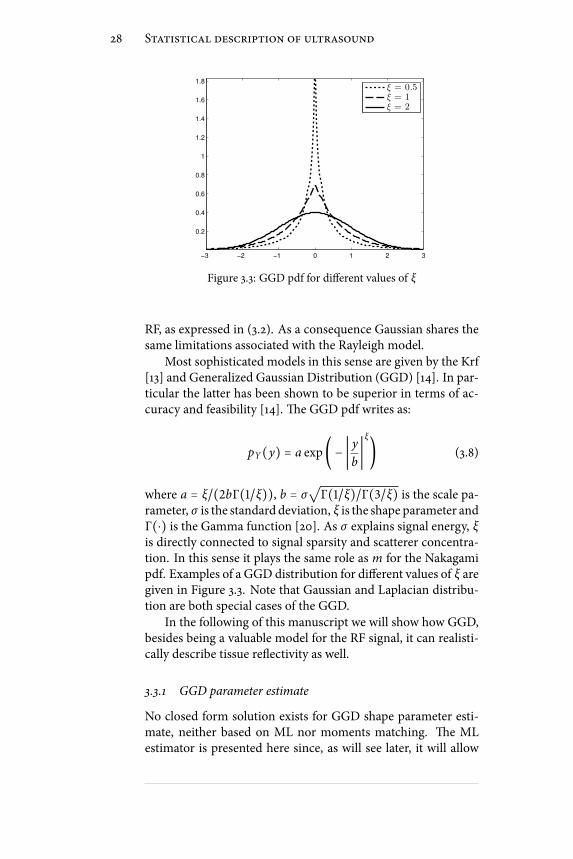
Most sophisticated models in this sense are given by the Krf[13] and Generalized Gaussian Distribution (GGD) [14]. In par-ticular the latter has been shown to be superior in terms of ac-curacy and feasibility [14]. e GGD pdf writes as:
pY(y) = a exp( − ∣ yb∣ξ) (3.8)
where a = ξ/(2bΓ(1/ξ)), b = σ√Γ(1/ξ)/Γ(3/ξ) is the scale pa-rameter, σ is the standard deviation, ξ is the shape parameter andΓ(⋅) is the Gamma function [20]. As σ explains signal energy, ξis directly connected to signal sparsity and scatterer concentra-tion. In this sense it plays the same role as m for the Nakagamipdf. Examples of a GGD distribution for dierent values of ξ aregiven in Figure 3.3. Note that Gaussian and Laplacian distribu-tion are both special cases of the GGD.
In the following of this manuscript we will show how GGD,besides being a valuable model for the RF signal, it can realisti-cally describe tissue reectivity as well.
3.3.1 GGD parameter estimate
No closed form solution exists for GGD shape parameter esti-mate, neither based on ML nor moments matching. e MLestimator is presented here since, as will see later, it will allow

3.4. Comparison 29
Blood Region
(a)
Muscle Region
(b)
Figure 3.4: Selected regions of interest: (a) blood pool internal tothe ventricle, (b) portion of the cardiac muscle.
us to design a deconvolution framework consistent with the Ex-pectation Maximization framework.
e ML ξ estimate of ξ is obtained from solving:
N
ξ+NΨ(1/ξ)
ξ2−
N∑k=1
(∣xk ∣b)ξ log( ∣xk ∣
b) = 0 (3.9)
and then
b = ( ξ
N
N∑k=1
∣xk ∣ξ)1/ξ
. (3.10)
e Newton method in [21] can be used to solve (3.9).
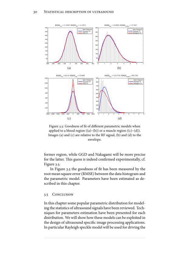
3.4 Comparison
We present here an example of the tting capability of the dis-tributions described in this chapter for the case of cardiac ultra-sound data. In particular, data from two regions are considered,corresponding to the blood pool inside the le ventricle and thecardiac muscle, see Figure 3.4. ese two kind of tissues exhibitdierent scattering properties, in particular blood regions areclose to the fully developed model, while muscle areas are pre-Rayleigh. From this information one can anticipate that Gaus-sian and Rayleigh distributions will provide accurate ts for the
30 Statistical description of ultrasound
−400 −300 −200 −100 0 100 200 300 4000
50
100
150
200
250
300
350
400
450
RMSEGA
= 11.9367 | RMSEGG
= 11.1873
data histogram
Gaussian Fit
GGD Fit
(a)
0 1 2 3 4 5 6 70
50
100
150
200
250
300
350
400
RMSERA
= 14.0956 | RMSENAKA
= 13.7447
data histogram
Rayleigh Fit
Nakagami Fit
(b)
−2500 −2000 −1500 −1000 −500 0 500 1000 1500 20000
200
400
600
800
1000
1200
1400
RMSEGA
= 84.18 | RMSEGG
= 35.9607
data histogram
Gaussian Fit
GGD Fit
(c)
0 1 2 3 4 5 6 7 8 90
100
200
300
400
500
600
700
800
900
RMSERA
= 119.3736 | RMSENAKA
= 89.1704
data histogram
Rayleigh Fit
Nakagami Fit
(d)
Figure 3.5: Goodness of t of dierent parametric models whenapplied to a blood region ((a)–(b)) or a muscle region ((c)–(d)).Images (a) and (c) are relative to the RF signal, (b) and (d) to the
envelope.
former region, while GGD and Nakagami will be more precisefor the latter. is guess is indeed conrmed experimentally, cf.Figure 3.5.
In Figure 3.5 the goodness of t has been measured by therootmean square error (RMSE) between the data histogram andthe parametric model. Parameters have been estimated as de-scribed in this chapter.
3.5 Conclusion
In this chapter some popular parametric distribution formodel-ing the statistics of ultrasound signals have been reviewed. Tech-niques for parameters estimation have been presented for eachdistribution. Wewill show how thesemodels can be exploited inthe design of ultrasound specic image processing applications.In particular Rayleigh speckle model will be used for driving the

3.5. Conclusion 31
evolution of an active contour addressing the recognition ofmy-ocardial boundaries from echocardiography; GeneralizedGaus-sian distribution will be used as prior distribution for modelingthe tissue reectivity in the derivation of a Maximum a Posteri-ori deconvolution framework; Nakagami parameters will be ad-opted, along with GGD ones, for characterizing dierent scat-terer concentrations from tissue mimicking phantoms.


II - Restoration of Ultrasound Images


Summary
It has been shown that, at least in the weak scattering ap-proximation, the ultrasound image can be expressed as thelinear convolution of the tissue response with the system
PSF.e non-negligible spatially-variant extent of the PSF is oneof the main causes to the limited quality of ultrasound frames,whichmakes sometimes opt formore onerous potentially harm-ful but more reliable imagingmodalities. In this context, decon-volution is commonly proposed in literature as a post processingtool for improving resolution and contrast of ultrasound imagesby removing to the maximum extent possible the blurring ef-fect associated with the PSF. e problem is oen tackled as anl 2-norm or l 1-norm constrained optimization task.
In this part of the thesis, an alternative application of decon-volution is considered instead, i.e. its use as a pre-processing stepfor potentiating ultrasonic tissue characterization. is proce-dure relies on the quantitative analysis of the echo signal to inferinformation about the tissue structure. e feasibility of theseapproaches for discriminating healthy tissues against cancerousones from breast and prostate ultrasound has been largely doc-umented. From the observation that the reectivity of a tissuecarries cleaner information on its structure than the raw echosignal does, the possibility of exploiting the deconvolved imagerather then the unprocessed one for tissue characterization is in-vestigated. From this perspective, standard deconvolution algo-rithms reveal strong limitations, principally ascribed to the sim-plied tissue models they make use of. Indeed, though theseare sucient for producing appreciable image quality improve-ment, they otherwise induce a statistical bias in the statistics ofthe restored reectivity, making it unusable for characterizationpurposes.
Hereto, a novel deconvolution method for ultrasound im-ages has been developed and is described. e algorithm is de-
35
36 Summary
rived on the base of a non-standard statistical model for the tis-sue response, dened by the Generalized Gaussian Distribution.By means of two distinct parameters, called scale and shape pa-rameter, this distribution allows sequences of arbitrary energyand sparsity to be generated, and is therefore adequate for pro-viding an accurate description to the most general tissue struc-tures. Deconvolution is then tackled as a Maximum a Posterioriestimate, in which tissue reectivity is restored along with anestimate of the associated scale and shape parameter. An Ex-pectation Maximization framework is designed to address thistask. An evaluation of performance will be presented on exper-imental data from several tissue-mimicking phantoms having awell-dened particle concentration. ese studies will show im-provements in classication accuracy of up to the 20% and thesuperiority of the proposed algorithm over standard ones.
is thesis part proceeds as follows. edeconvolution prob-lem is formulated in Chapter 4 where most common solutions,as Wiener lter and l 1-norm optimization, are presented. eoriginal restoration scheme will be nally derived and evaluatedin Chapter 5.

Chapter 4Deconvolution problem
Connaturatedwith every imaging technique is a discrep-ancy between the true scene and the imaged one. eentity of these errors is dependent on the features of the
sensing devices as well as on the physical phenomena underly-ing the image formation process. Many of these elements can bereasonably accounted for by linear models. Although not rigor-ous, they represent a commonly accepted approximation for thelargest majority of applications. Under this assumption of lin-earity, the observed image can be expressed as the linear convolu-tion of the true image with a linear blurring kernel. e problemof image deconvolution, or, equivalently, restoration or deblur-ring, naturally arises from this scenario, and has its goal in theenhancement of image resolution and contrast by the restora-tion of an estimate of the true image. Image restoration is a verycommon problem in image processing, encountered in a widevariety of technical areas as astronomy, seismology, microscopyand medical imaging. See [22, chap. 1] for a review.
In this chapter the problem of medical ultrasound restora-tion is addressed. In §4.1 the problem is dened and some ma-jor issues implied by the peculiar nature of ultrasound are dis-cussed. In §4.2 the simple predictive deconvolution scheme ispresented alongwith itsmain limitations. In §4.3 it is shownhowdeconvolution can be formalized as a Bayesian inference prob-lem and themost popular related solutions (Wiener ltering andl 1-norm deconvolution) are presented. As predictive deconvo-lution is a completely blind technique, Bayesian techniques re-quire the availability of an estimated PSF instead. Hereto in §4.4several techniques for estimating ultrasound PSFs from the
37
38 Deconvolution problem
backscattered echo are discussed. e chapter concludes in §4.5.
4.1 Problem statement
As shown in Chapter 2, as long as imaging of so tissues is con-cerned, the rst order Born approximation can be applied andthe radio-frequency (RF) image y can be expressed as:
y[n.m] = ∑k , l
h[n, k;m, l]x[k, l] + ν[n,m] (4.1)
where x represents the tissue reectivity function, h is the trans-ducer’s Point Spread Function (PSF) and ν is Gaussian measure-ment noise. e problem of image restoration is then dened asproducing an estimate of x from the observation y. In the se-quel we will address some very important issues arising in thecase of ultrasound images, making the restoration problem forthis class of images particularly challenging.
At rst we note that the model (4.1) is intrinsically non sta-tionary, indeed h is allowed to vary its shape when measuredat dierent locations. is is indeed the case of medical ultra-sound, where the system PSF may change considerably on theimaged plane. is spatial variability is principally connectedwith the beamforming performed by the array in order to havebetter resolved images, but is also due to the presence of the tis-sue itself, whose attenuating and dispersive action on the acous-tic eld propagation is known to be highly frequency dependent.ese issues have been more exhaustively explained earlier in§2.5 of this manuscript.
ese considerations not only conrm that a spatially vari-ant PSF must be considered in a realistic signal model, but in-troduce a further issue. is consists in the fact that, althoughspatial variations associatedwith systemdependent eects couldtheoretically be a priori modeled given a perfect knowledge ofthe acquisition modality, instead this is not the case for tissuedependent ones. Indeed they are intrinsically depend on thestructural properties of the insonied medium, which, exclud-ing very controlled experimental setups, are completely unpre-dictable. As a result, the blurring term h in (4.1) is also an un-known of the problem. e class of deconvolution problems inwhich none or little information is available on the blurring ker-nel is referred in literature as blind deconvolution [22, 23].
eblinddeconvolution problemcanbe tackled in twoways.erst consists in estimating the tissue reectivity and the trans-

4.2. Predictive deconvolution 39
ducer PSF simultaneously. e second approach is instead to es-timate the PSF rst, followed by using such an estimate to solvethe deconvolution problem in a non-blind manner. We antici-pate that this second solution is fairly themost common. Indeed,as we will see, these methods are free from strong hypothesis onthe signal statistics implied by the former ones, and allow formore realistic tissue models to be taken into account.
Among the completely blind deconvolution strategies pre-dictive deconvolution represents a very popular alternative. istechnique is described in the next section.
4.2 Predictive deconvolution
Predictive deconvolution was rst introduced in [24] for decon-volving seismograms obtained in reection seismology. Seis-mology and medical ultrasound represent two techniques in-spired by the same intent, that is to say to characterize a propa-gating medium through the echo returned aer an acoustic so-licitation of the same. In the former case air guns are employedas sources and the medium is the earth crust, in the latter piezo-electric transducers are used to image biological tissues. esesimilarities motivate the tentative to apply tools developed forthe processing of seismic signals to the treatment of medicalones. In particular, predictive deconvolution for medical ultra-sound has been investigated in fewworks, as [25, 26]. e readeris addressed to [27] for an extensive dissertation on the employ-ment of predictive techniques, and adaptive lters in general, formedical ultrasound restoration.
Predictive deconvolution assumes an autoregressive (AR)model for the echo signal y, i.e.
y[n] = P∑k=1
a[k]y[n − k] + x[n] (4.2)
where y and x have the samemeaning as in (4.1). e coecientsa[k] are called auto-regressive coecients of y, and P is the or-der of the model. In this context x is also called excitation of theautoregressive model, and must be white noise. Note that a onedimensional formulation has been used. Indeed, in medical ul-trasound, the common practice is to apply blind deconvolutiontechniques of this kind only along the axial direction of propa-gation [22, 25].
40 Deconvolution problem
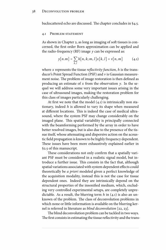
z PREDICTORy[n] y[n]^
+-
e[n]-1
Figure 4.1: Predictive deconvolution.
Note that (4.2) is equivalent to y[n] = (h ∗ x)[n] if:H(z) = Y(z)
X(z) = 1
1 −∑p
k=1 a[k]z−k (4.3)
where H(z) = ∑n h[n]z−n is the Z-transform [8, chap. 3] of thePSF h. at is to say when h is an all-pole, minimum-phase lter[8, pp. 280–290].
e scheme for predictive deconvolution is represented inFigure 4.1. e function of the predictive block is to produce aguess y[n] of y[n] given a set of its delayed samples. In practiceit is implemented as a linear nite impulse response (FIR) lterwith taps w = [w1 ,⋯,wM], so that:
y[n] = M∑k=1
w[k]y[n − k] (4.4)
e values of the coecients is computed so to satisfy the opti-mal prediction condition:
w∗ = argminw
E(e2[n]) (4.5)
where e[n] = y[n] − y[n] is the prediction error and E⋅ rep-resents the statistical expectation.
It is immediate to show that, when y is an autoregressiveprocess, the so obtained linear prediction coecients providein eect an estimate of the autoregressive parameters a. As aconsequence, the prediction error e[n] is an estimation of theexcitation process x, that is to say the deconvolved trace.
A common way to compute the prediction coecients in(4.5) is by solving the associated Wiener-Hopf equations [28,chap. 6]. is solution is optimal provided that a consistent es-timate of the autocorrelation function of the input trace y[n]can be computed. is implies that a stationary time realiza-tion of sucient duration is available. Unfortunately, medicalultrasound signals cannot be considered stationary or, at least,

4.2. Predictive deconvolution 41
stationarity hypothesis can bemade only on small segments. In-deed, though the time invariant autoregressive model has beenintroduced in (4.2) for conformity with the literature onAR pro-cesses, a much more realistic model would instead take time-variant coecients into account, i.e.
y[n] = P∑k=1
a[n; k]y[n − k] + x[n] (4.6)
As a consequence not a xed set of AR coecients must be esti-mated from an entire ultrasonic scan line, otherwise they shouldbe adaptively updated so to second to the time-variant proper-ties of the signal. A consolidated alternative for dealing with thisclass of signals is represented by adaptive ltering techniques.
4.2.1 RLS algorithm for linear prediction
Adaptive lters are lters in which taps are recursively updatedthroughout all the acquisition process in order to compensatefor time varying changes of acquisition system or propagatingchannel. e literature on adaptive lters is extremely wide, see[28] for an exhaustive dissertation. e most classical solutionsfor the updating rule are the Least Mean Square (LMS) algo-rithm [28, chap. 9] and the Recursive Least Squares (RLS) algo-rithm [28, chap. 13]. In particular, the second is known to ensurebetter performance both in terms of convergence and trackingcapabilities.
e RLS algorithm relies on the following approximation ofthe cost function Ee2[n]:
Γe2[n] = n∑k=1
λn−k e2[n] (4.7)
where λ ∈ [0, 1] is called the forgetting factor and represents thememory of the lter. In particular, values of λ close to 1 cor-respond to considering segments of higher duration: this im-proves the coecients estimate when stationarity assumptionscan be made but limits the tracking capabilities for highly nonstationarity signals. Symmetrically, small values of λ improvethe dynamic behavior on one side, but make the approximationgiven by Γ more dramatic on the other, so degrading the consis-tency of the estimated coecients. As a consequence, λ has tobe carefully tuned in relation with the application at hand.

42 Deconvolution problem
Table 4.1: Summary of the RLS algorithm
Initialization: P[0] = δ−1 ⋅ I, w[0] = 0,For n= 1,2,..., compute:
k[n] = λ−1P[n − 1]u[n]1 + λ−1uT[n]P[n − 1]u[n] ,
ξ[n] = y[n] − wT[n − 1]u[n],w[n] = w[n − 1] + k[n]ξ[n],P[n] = λ−1P[n − 1] − λ−1k[n]uT[n]P[n − 1],
Before going through the description of the algorithm it isuseful to introduce here the some variables. We dene
u[n] = [y[n − 1],⋯, y[n −M]]T (4.8)
the input to the predictor, so that y[n] = wTu[n];Φ[n] = n∑
i=1
λn−iu[i]uT[i] (4.9)
the estimate of the autocorrelation matrix and
z[n] = n∑i=1
λn−iu[i]y[i] (4.10)
is the estimate of the crosscorrelation vector between the inputsequence u and y.
e solutionw∗, that minimizes (4.7), is then obtained fromthe relation
w∗(n) = Φ−1(n)z(n) (4.11)
In practice no matrix inversion is needed and the matrix in-version lemma is used instead [28, pp. 565]. A summary of theRLS algorithm is reported in Table 4.1. e RLS algorithm is avery consolidated framework in adaptive lter theory, the inter-ested reader may nd an exhaustive derivation e.g. in [28].
4.2.2 Limitations of the approach
Several pros and cons go along with the predictive deconvolu-tion technique when employed in the context of medical ultra-

4.2. Predictive deconvolution 43
sound. ey have been mentioned throughout the text but it’suseful to summarize them here. e main advantages are:
• e small computational complexity. In fact, they relieson simple ltering techniques for which several simplehardware implementations could be thought or borrowedfrom the telecommunications literature. Moreover eachscan line is typically processed independently from theadjacent one, as a consequence this intrinsic parallelismcould be exploited for considerably reducing the total costassociated to the deconvolution of the entire image. Forthese reasons, adaptive ltering deconvolution techniquesare with no doubts the most promising candidates as longas real-time processing is pursued.
• ey are completely blind. As a consequence no PSF es-timation strategy is needed. We will see in the followingthat several complications are associated with these esti-mation techniques.
• e intrinsic non-stationarity of the system is directlytaken into account as the model coecients are contin-uously updated.
Limitations are mainly due to the assumptions at the base ofthe predictive deconvolution scheme. Indeed, if they can be ad-equate in reection seismology or in some telecommunicationapplication, they are instead too severe for medical ultrasound.ese are:
• e PSF cannot be well represented by an all-pole systemas the one in (4.3). Indeed the AR model is useful formodeling random signals that possess peaky power spec-tral densities. When more complex situations with broadpeaks or sharp nulls exist, which is the case in medicalultrasound, more general models should be alternativelyused, as autoregressive moving average (ARMA). eseconcept is illustrated in Figure 4.2, where the inadequacyof the AR model for representing the actual shape of thespectrum of an experimental PSF is evident, along withthe better approximation oered by anARMAmodel. Un-fortunately, several shortcomings accompany the employ-ment of ARMA schemes, which limit their use as well.At rst much onerous model estimation procedures are

44 Deconvolution problem
10 20 30 40 50 60 70 80
−3
−2
−1
0
1
2
3
Experimental PSF
(a)
0 0.2 0.4 0.6 0.8 10
0.1
0.2
0.3
0.4
0.5
0.6
0.7
0.8
0.9
1
Power Spectrum
(b)
0 0.2 0.4 0.6 0.8 10
0.1
0.2
0.3
0.4
0.5
0.6
0.7
0.8
0.9
1
AR model
(c)
0 0.2 0.4 0.6 0.8 10
0.1
0.2
0.3
0.4
0.5
0.6
0.7
0.8
0.9
1
ARMA odel
(d)
Figure 4.2: (a) Experimental PSF obtained as the response of ametal wire immerse in a water tank. (b) Power spectrum of theexperimental pulse. (c) Power spectrum of the AR estimate. (d)
Power spectrum of the ARMA estimate. For the AR the best t hasbeen obtained for an lter length of M=4. For the ARMA both
number of zeros and poles was equal to 5.
needed. Moreover, adaptive strategies cannot be formal-ized [22, pp.185–190], which preclude the time variance ofthe system from being correctly taken into account.
• Experimental PSFs are known to have a non-negligiblelateral extent, which makes the 1-D model highly inade-quate. For this reason, modern deconvolution techniquesall exploit more realistic 2-D [29, 30, 31], when not 3-D[32, 33], PSF models.
• Assuming the tissue reectivity to be a white Gaussianprocess is an unacceptable simplication for biological tis-sues. At rst, variations in the echogenicity proles are theimmediate consequence of the simultaneous presence ofdierent biological structures encountered inside realisticimages, which make a white process a highly inadequate

4.3. Maximum a posteriori deconvolution 45
model. Moreover more realistic scattering conditions canbe accounted for by more exible distributions than theGaussian, as detailed in Chapter 3. ese concepts will befurther addresses in the next sections and more diuselyin the next Chapter.
e aforementioned limitations justify the fact that very fewauthors spent big eorts in the investigation of predictive de-convolution schemes for medical ultrasound. e most com-mon strategy is instead to exploit dierent approaches, relyingupon statistical estimation and convex-optimization theory. Atthe same time we further stress that techniques based on adap-tive lters are instead the most promising alternative when on-line processing is needed.
4.3 Maximum a posteriori deconvolution
Unlike predictive deconvolution, this kind of techniques addressthe blind deconvolution problem in a two step scheme: the PSFh is estimated rst and subsequently the task is tackled in a non-blind manner. In this section we describe the most commontechniques for the latter step. Possible ways for estimating thePSF from the echo image are described later in this chapter.
4.3.1 Problem formulation
For compactness of notation, let’s rewrite the signal model in(4.1) with the common matrix-vector notation [34]:
y = Hx + ν (4.12)
where y, x and ν are vectors obtained aer lexicographical or-dering from the corresponding images and H is the matrix as-sociated to the blur [34, Appendix A]. Specically, assuming ageneric N ×M RF-image, then y is the NM × 1 vector obtainedby stacking each column under the previous one and H is anNM × NM matrix. With this formalism, deconvolution trans-lates into providing a reasonable solution x to (4.12).
We remark that PSF shape variation requires a spatially vari-ant blur to be taken into account within an accurate deconvolu-tion framework. ough a pointwise variant kernel could theo-retically be embedded in (4.12), this would require productsHx
andHTx to be computed explicitly, thereby making deconvolu-tion computationally unfeasible. Hereto, the simplest approach

46 Deconvolution problem
is to assume a slowly varying PSF [31, 29, 35], and hence well ap-proximated by a piecewise constant function. In this case, thedata image can be divided into a number of segments, whosesize is chosen to be small enough to guarantee that each of thesegments is formed by a stationary convolution with a dierentPSF.
With this model, the following expressions holds [36]:
H = K∑k=1
DkHk , HT = K∑k=1
HTk Dk (4.13)
where Hk denotes the spatially invariant PSF associated to thekth segment and Dk is the diagonal matrix determining the in-terpolation between the kth region and the neighboring ones(cf. Appendix B). Since each of the Hk is Block Toeplitz withToeplitz Blocks, then products of the type Hx and HTx can beeciently implemented via Fast Fourier Transform [36]. Detailsabout structure ofH are given in Appendix B of this manuscript.
4.3.2 Bayesian framework
Image deconvolution is oen tackled as a statistical inferenceproblem [37, 38, 35]. In this case, vectors y, x and ν of the modelin (4.12) are treated as single realizations of random processes,to which a suitable probability density function (pdf) p(⋅) is as-signed. In this context, the two most common estimationparadigms areMaximumLikelihood (ML) andMaximumaPos-teriori (MAP), respectively seeking the realization of xmaximiz-ing the log-likelihood ln[p(y∣x)] and the log-posterior ln[p(x∣y)],see [16].
If the noise is modeled as zero mean white Gaussian withvariance σ 2
n :
pν(ν) = 1(2πσ 2n)N exp( − 1
2σ 2n
∣∣ν∣∣22) (4.14)
then p(y∣x) = pν(y −Hx):p(y∣x) = 1(2πσ 2
n)N exp( − 1
2σ 2n
∣∣y −Hx∣∣22) (4.15)
where N is now the total number of samples in the image. From(4.15) one can derive that ML estimate corresponds to the leastsquares solution to (4.12), minimizing the error norm ∣∣y−Hx∣∣22.
4.3. Maximum a posteriori deconvolution 47
As known, this problem is directly solved by pre-multiplying ywith the pseudo-inverse of H, i.e. (HTH)−1HT . Unfortunately,in medical ultrasounds, like in any other measurement tech-nique, the system matrix H is necessarily ill-conditioned. isfact is directly connected to the band-limitedness of acquisitionsystem impulse response. Hence, inverse ltering results in anunacceptable amplication of the out-of-bandnoise components.In this context, MAP technique provides a way to cope with theill-posedness of the restoration problem by including further in-formation in the estimation task. In particular, it requires a priormodel p(x) to be assigned to the desired solution. Using theBayes rule p(x∣y) ∝ p(y∣x)p(x), the MAP estimate of x thenwrites as:
xMAP = argminx
1
2σ 2n
∣∣y −Hx∣∣22 − log p(x) (4.16)
where p(x) reects the prior belief about x, acting as a regulariz-ing constraint in the inversion of (4.12). In practice, reectivitysamples x i are modeled as independent identically distributedrandom variables, so that p(x) = ∏ p(x i). e two reectivitymodels by far the most common in deconvolution literature, i.e.Gaussian and Laplacian, are discussed in the next Section.
4.3.3 Gaussian model
If x obeys a multivariate Gaussian distribution with zero meanand co-variance matrix ExTx = Σx:
px(x) = 1(2π)1/2∣Σx∣1/2 exp1
2xTΣ−1x x (4.17)
then the restoration problem maps into a (weighted) l 2-normoptimization task:
log p(x∣y)∝ 1
2σ 2n
∣∣y −Hx∣∣22 + 1
2xTΣ−1x x (4.18)
e solution∇x log p(x∣y) = 0 is given by:
x = (HTH + σ 2nΣ−1x )−1HTy =Wy (4.19)
whereW is the well known Wiener lter [34, Ch.8]. Due to thesize of the problem thematrix inversion involved by (4.19) is notfeasible in a direct way. It is hereto common to adopt iterative
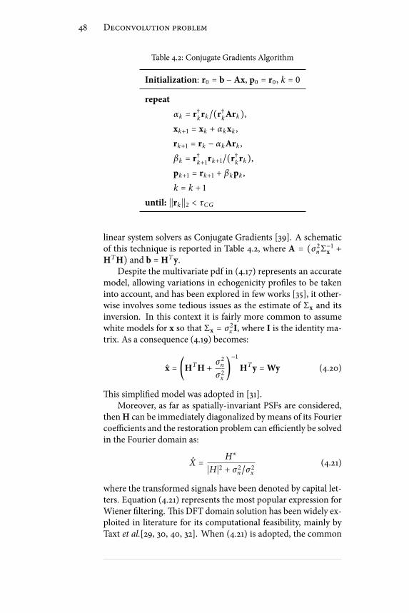
48 Deconvolution problem
Table 4.2: Conjugate Gradients Algorithm
Initialization: r0 = b −Ax, p0 = r0, k = 0repeat
αk = r†krk/(r†kArk),xk+1 = xk + αkxk ,
rk+1 = rk − αkArk ,
βk = r†k+1rk+1/(r†krk),pk+1 = rk+1 + βkpk ,
k = k + 1until: ∣∣rk ∣∣2 < τCG
linear system solvers as Conjugate Gradients [39]. A schematicof this technique is reported in Table 4.2, where A = (σ 2
nΣ−1x +
HTH) and b = HTy.Despite the multivariate pdf in (4.17) represents an accurate
model, allowing variations in echogenicity proles to be takeninto account, and has been explored in few works [35], it other-wise involves some tedious issues as the estimate of Σx and itsinversion. In this context it is fairly more common to assumewhite models for x so that Σx = σ 2
x I, where I is the identity ma-trix. As a consequence (4.19) becomes:
x = (HTH +σ 2n
σ 2x
)−1HTy =Wy (4.20)
is simplied model was adopted in [31].Moreover, as far as spatially-invariant PSFs are considered,
thenH can be immediately diagonalized by means of its Fouriercoecients and the restoration problem can eciently be solvedin the Fourier domain as:
X = H∗∣H∣2 + σ 2n/σ 2
x
(4.21)
where the transformed signals have been denoted by capital let-ters. Equation (4.21) represents the most popular expression forWiener ltering. is DFT domain solution has been widely ex-ploited in literature for its computational feasibility, mainly byTaxt et al.[29, 30, 40, 32]. When (4.21) is adopted, the common

4.3. Maximum a posteriori deconvolution 49
way do deal with non stationarity of the PSF is to deconvolvesingle sub-images and then to merge the results. Taking care ofavoiding block artifacts by suitably overlapping the image seg-ments.
Despite the computational eciency, DFT-domain Wienerlter yields sub-optimal results because the complex exponen-tials that comprise the basis of the DFT have poor spatial lo-calization, so that modications to individual DFT coecientsof x result in global changes to the entire image that are oenmanifested as Gibbs ringing artifacts [41]. Moreover, as a lin-ear lter, Wiener solution is incapable of interpolating the out ofband information that was lost during the image formation pro-cess, so producing oversmoothed solutions [31]. e reader maynote that these shortcomings are shared with the predictive de-convolution scheme described at the beginning of this Chapter.Indeed, although derived in dierent ways, these two techniqueshave much in common: in both cases a Gaussian model for thereectivity is assumed, which, as we will discuss later, in fairlytoo simplied for a real tissue, moreover, in both cases a linearregularized approximation of inverse lter is produced, whichgoes along with the oversmoothing and the ringing phenomena.
ese considerations motivate the need for alternative re-ectivitymodels. In this context Laplacian distribution has beenthe most popular.
4.3.4 Laplacian model
If a Laplacian model is assumed for the reectivity:
p(x i) = 1√2σ 2
x
exp( −√ 2
σ 2x
∣x i ∣) (4.22)
then the restoration problem in (4.16) translates into an l 1-normoptimization task [31]:
x = argminx
1
2σ 2n
∣∣y −Hx∣∣22 + λ∣∣x∣∣1 (4.23)
where λ = √2/σx and ∣∣x∣∣1 = ∑ ∣x i ∣ denotes the l 1-norm. eoptimization problem dened by (4.23) does not have a closedform solution, and must be handled with iterative convex opti-mization schemes [31, 42]. A possible solution to (4.23) will beaddressed in the next Chapter, where a general framework forthe solution of l p-norm problems will be described.

50 Deconvolution problem
−3 −2 −1 0 1 2 3
0.05
0.1
0.15
0.2
0.25
0.3
0.35
GAUSSIAN PDF
(a)
−3 −2 −1 0 1 2 3
0.1
0.2
0.3
0.4
0.5
0.6
LAPLACIAN PDF
(b)
Figure 4.3: Comparison between Gaussian and Laplacian pdfs.
e literature on l 1-norm optimizations is wide, indeed itis the standard procedure solving linear systems when the so-lution is known to be sparse. In the context of medical ultra-sound deconvolution, Laplacian prior was rst introduced byMichailovich et al.[31, 43]. It has to be noted that Laplacian pdfpossesses heavier tails than the Gaussian one and, hence, thereis a greater allowance for a few occasional large-amplitude sam-ples to occur, cf. Figure 4.3. For this reason, such a model is bet-ter suited for representing more realistic tissues with diusivescatterers superimposed with sparse specular reectors. A com-parison betweenWiener and l 1-norm deconvolution is given inFigure 4.4, where the increased sparsity associated to the Lapla-cian prior is evident, along with the oversmooting eect causedby Wiener ltering.
4.3.5 Advantages and shortcomings
esemaximumaposteriori techniques represent themost com-mon restoration strategies for medical ultrasound. An overviewof the literature concerning ultrasound images restoration pro-duced in the last 15 years is summarized in Table 4.3. osemethods are directly derived on the base of the optimizationtasks derived in the previous section, or on slight modications.From the second column of the Table is evident how in somecase working on the in-phase/quadrature (IQ) signal is preferredthan on the raw RF. is is due to the fact that, aer demodu-lation, the IQ signal can be downsampled without introducingaliasing eects. e downasmpling factor is dependent on theratio between the transducer’s bandwidth and the sampling fre-quency (factors of 4-5 are oen feasible with standard acquisi-

4.3. Maximum a posteriori deconvolution 51
original
50 100 150
50
100
150
200
250
300
350
400
(a)
wiener
50 100 150
50
100
150
200
250
300
350
400
(b)
laplacian
50 100 150
50
100
150
200
250
300
350
400
(c)
Figure 4.4: Comparison between wiener and laplaciandeconvolution relative to a prostate scan acquired with Trans
Rectal Ultrasound (TRUS).
tion setups). is is highly desirable as standard deconvolutionalgorithm as the one discussed above mostly have a computa-tional complexity which raises with the square of the number ofsamples.
Main advantages of MAP techniques include:
• Twodimensional [30] or even three dimensional [32] PSFscan be accounted for.
• No assumption is made on the PSF, neither on the num-ber of zeros or poles, neither on the position of the zeroson the complex plane. In particular bothminimum phase(all zeros and poles inside the unit circle) andmixed phase[8] PSF can be considered. In this context we will see thatthis second hypothesis is the more realistic for ultrasoundpulses, which involve several complications in the PSF es-timation procedure.
• More advanced models than white Gaussian can be as-sumed for the tissue reectivity. In particular a degree ofcorrelation among samples can be introduced, as in [35],

52 Deconvolution problem
Table 4.3: Literature Overview on Medical UltrasoundDeconvolution
WORK METHOD
Signal PSF 1 Optimization
Abeyratne [44](1995)
1D-RF Estimated (HOS)Wiener DFT(4.21)
Taxt [40](1999)
1D-RF Estimated (H)Wiener Block(4.21)
Taxt [30](2001)
2D-IQ Estimated (H)Wiener Block(4.21)
Taxt [32](2001)
3D-RF Estimated (H)Wiener Block(4.21)
Michailovich [45](2003)
1D-RF Estimated (GH)Wiener Block(4.21)
Taxt [29](2004)
2D-IQ Estimated (H)Wiener Block(4.21)
Michailovich [31](2005)
2D-IQ Estimated (GH) l 1-norm (4.23),Wiener (4.20)
Jiřík [46](2006)
2D-RF Estimated (H)Wiener DFT(4.21)
Ng [35](2007)
2D-IQSimulated:FieldII [6]
Iterative Wiener(4.19)
Michailovich [43](2007)
2D-IQIterativerenement of GHestimate
Hybrid.l 1-norm.
1 When an estimated PSF is used, the following notation is adopted: HOSfor the cumulants-based estimate in §4.4.1, H for the cepstrum estimatein §4.4.2, GH for the generalized homomorphic estimate in §4.4.3.
where piecewise-smooth echogenicity variations due tothe presence ofmultiple tissues in the image are taken intoaccount by considering a non-whitemultivariate distribu-tion for the reectivity. Moreover, the hypothesis of Gaus-sianity can be disregarded aswell. is is done for instancewith the Laplacian model, but this concept will be furtherexpanded in the next Chapter.
Main limitations include:
• An increased computational cost, in particularwhenmorecomplex scheme than Wiener are employed. As a conse-quence, though considerable speed ups could be obtainedthanks to ecient implementations on dedicated hard-ware platforms or on GPUs, these tools are not promising

4.4. PSF estimation 53
candidate as long as real-time processing is the principalgoal.
• Although PSF estimation strategies have received a greatattention among several authors [29, 31, 45] this step stillremain tedious. In particular this ismotivated by the needof phase unwrapping procedures when non-minimumphase PSFs are considered. As long as ultrasounds areconsidered this operation is particularly challenging dueto the high and rapid variations of the signal phase, whichmake standard phase unwrapping algorithms developedfor other image modalities as MRI [47] of little use.
4.4 PSF estimation
As mentioned, deconvolution of ultrasound images is a blindproblem and MAP techniques cope with this fact by estimatingthe PSF from the RF image, and then use the obtained estimatewithin a non-blind setting. As the image formation is known tobe non stationary, the common solution is to partition the im-age axially into segments small enough to consider the processlocally stationary and then to estimate a dierent PSF on eachsegment. e global blurring operator is then to be built as in(4.13).
e literature on PSF estimation techniques is wide. esemethods can be grouped into threemain classes, whichwebrieyresume in this section. e reader is addressed to [22, chap. 5]for a more complete review on the subject. In order to keep thefollowing discussion uent let’s introduce here the variables tobe used throughout the rest of the section, see Table 4.4.
4.4.1 Higher-Order Statistic technique
is method was rst proposed in [44] for 1D signals. It re-lies on the following hypotheses: the psf h is deterministic andmixed-phase, the reectivity x is stationary zero-mean and non-Gaussian, the noise ν is stationary white Gaussian. Under theseassumptions the bispectrum of y can be written as [48]:
Cy(ω1 ,ω2) = Cx(ω1 ,ω2)H(ω1)H(ω2)H∗(ω1+ω2)+Cν(ω1 ,ω2)It can be shown that, if ν is white Gaussian then Cν = 0. More-over, if x is white non-Gaussian then its bispectrum is simply a

54 Deconvolution problem
Table 4.4: List of Symbols for PSF Estimate1
symbol definition description
G[ω] F (g[n]) spectrum
G[ω1 ,ω2] F2D (g[n,m]) 2D spectrum
G[ω1 ,ω2] logG[ω1 ,ω2] log-spectrum
cg[τ1 , τ2] Eg[n]g[n + τ1]g[n + τ2] 3-rd ordercumulant
Gg[ω1 ,ω2] F2D (cg[τ1 , τ2]) bispectrum
g[n,m] F−12D (G[ω1 ,ω2]) complexcepstrum
1 In this table F, F2D and F−12D represent Fourier transform, two-dimensional Fourier transform and inverse two-dimensional Fouriertransform respectively. In practice, as long as discrete time series are con-sidered, they are implemented by the Fast Fourier Transform (FFT) algo-rithm.
constant. erefore is evident how Cg is, a part of the multipli-cation by a constant, exclusively determined by the spectrum ofh, which suggests how the blur can be estimated from the bis-pectrum of the rf signal.
A strong limitation of this approach is that consistent esti-mates of higher order statistics require long stationary time re-alizations to be available. Otherwise all the desirable propertiesdescribed above may not hold and the resulting PSF estimate beinaccurate. As mentioned, this condition is never satised in areal world setting, where the echo rapidly varies its properties.Moreover 2D extension to these techniques is not straightfor-ward and may become fairly too computation demanding. Amuch more feasible and popular alternative is represented byhomomorphic techniques.
4.4.2 Homomorphic technique
Homomorphic deconvolution has been widely explored with acertain success by Taxt et al., see Table 4.3. e log-spectrum Y
4.4. PSF estimation 55
of y is:
Y(ω1 ,ω2) = log ∣X(ω1 ,ω2)∣ + log ∣H(ω1 ,ω2)∣++ j ∠H(ω1 ,ω2) +∠X(ω1 ,ω2) (4.24)
It can be shown that, at least withing the transducer bandwidth,both log ∣H∣ and∠H are reasonably smooth signals, while boththe power spectrum and the phase of x are spiky noise-like se-quences [49]. As a consequence, the spectrum of H can be re-trieved from Y by ltering both its real and imaginary parts.
Homomorphic techniques accomplish this separation in thecepstrum domain [8]. In particular, from (4.24) it is straight-forward to derive cy[n,m] = cx[n,m] + ch[n,m], where, forthe considerations above, ch is a fast converging sequences, withits energy conned at the origin of the cepstrum domain, whilethe energy of y is spread over the entire cepstrum domain dueto the non regularity of Y . Although the two sequences ch andcy may have a certain overlapping, this is usually neglected andthe cepstrum of the PSF ch is simply obtained by truncating thecepstrum cy of the echo signal [50, 29, 51].
4.4.3 Generalized homomorphic technique
Generalized homomorphic technique [31] also exploits dier-ent smoothing properties of H and X in order to retrieve a PSFestimate from (4.24). e main dierence is that smoothing isnot performed by truncation in the cepstrum domain, as in thetraditional homomorphic scheme, but by projection of both thereal and imaginary parts of (4.24) on a reduced resolution space.is is done bymeans ofwavelet ltering, where the signal statis-tics are taken into consideration in order to dene the optimalbasis and threshold. is technique is documented to outper-form the traditional one in [50] in terms of mean square recon-struction error and will be adopted in the following Chapter.
We conclude this section by noting that a major complica-tion goes along with homomorphic or generalized homomor-phic techniques, represented by the need of unwrapping thephase of Y before the PSF estimation procedure. As the phaseof ultrasound signals present very peculiar properties, makingstandard unwrapping tools developed for alternativeimagingmodalities likeMRI of little or no use at all [47], severalad hoc phase unwrapping algorithms have been proposed in lit-erature. A discussion on phase unwrapping is beyond the scope
56 Deconvolution problem
of this manuscript. Major contributors in this context are Strandand Taxt [52, 53] and Michailovich [49, 54]. Although good re-sults are documented, details about their implementation are of-ten le quite obscure. In the following chapter, as a compromisebetween feasibility of implementation and accuracy of results,we adopt the phase unwrapping technique described in [55].
4.5 Conclusion
In this chapter the problem of deconvolution for medical ultra-sound has been introduced. e principal techniques for tack-ling this task have been reviewed, with an emphasis on predic-tive deconvolution and Maximum a Posteriori approaches. Wementioned that predictive deconvolution, despite its computa-tional eciency, introduces several simplicationswhich are toosevere formedical ultrasound and, for this reason, it has receivedonly a limited attention. In particular, we have obtained some in-teresting results relative to the employment of predictive decon-volution within a Trans Rectal Ultrasound (TRUS) based Com-puter Aided Detection (CAD) tool for classication of prostatecancer [26, 56]. Otherwise, that project was marginal to the pri-mary doctoral research activity and wont be further detailed inthis manuscript.
e focus then dried to Maximum a Posteriori restorationtechniques, which represent the state of the art in medical ul-trasound and in image processing in general. Indeed, due totheir exibility, they allow suitably modeling the majority of tis-sue and system dependent eects involved in a real acquisition.In particularmost commonWiener lter and l 1-normoptimiza-tion have been dened. ose MAP techniques assume a prioriknowledge of the blurring kernel, i.e. the system PSF. As theproblem of deconvolution of medical ultrasound is blind, thecommon solution is to use estimates of the PSF obtained fromthe echo signal. Hereto the most classical estimation strategieshave been reviewed at the end of the chapter.
All the concepts here introducedwill be exploited in the nextchapter, where a novel algorithm for deconvolution of medicalultrasound will be derived.

Chapter 5Deconvolution and tissue characterization
Medical ultrasound represents a non-invasiveand cost-ecient imagingmodality. Beyond that, ul-trasound provides a precious tool for tissue charac-
terization since, from the analysis of the backscattered echo sig-nal, relevant information on structural properties of the insoni-ed tissue can be inferred, otherwise unaccessible from simplevisual inspection.
is principle is at the base of a consolidated research branchreferred as Ultrasonic Tissue Characterization (UTC). In par-ticular, it has been eectively exploited in a clinical context inthe development of ultrasound-based Computer Aided Detec-tion (CAD) schemes. e purpose of CAD is to support thephysician in the interpretation of ultrasound images and to assisthim in the decision-making process when suspicious situationsare encountered. Signicant results have been documented on arange of clinical applications, like prostate cancer recognition onTRUS [57], detection of suspicious masses in breast ultrasounds[58] and diagnosis of hepatic steatosis [59]. e computer out-put is derived from quantitative analysis of the echo signal. Inthis context, a large amount of features of dierent nature havebeen proposed in literature, which can be subdivided accordingto their contribution in highlighting specic tissue properties.
Tissue characterization based on the acoustic parameters suchas attenuation and backscattering coecients extracted fromradio-frequency (RF) echo signals has beenwidely studied. esequantities are commonly estimated by using one-dimensional[60] or two-dimensional [61] spectrum analysis of the RF sig-nal. Spectral features have proven to provide useful outputs for
57

58 Deconvolution and tissue characterization
diagnosis of diseases in various organs, like eye, prostate, breastand liver; see [62] for a comprehensive review. Besides the RF-spectrum analysis, many researchers have used texture featuresextracted from ultrasound B-scan images for characterizationpurposes. e initiative is that the speckle pattern in the ul-trasonic image can reveal structural information about the tis-sue. Usefulness of textural features within clinical settings hasbeen largely documented, e.g. for prostate carcinoma diagnosis[63, 26], evaluation of liver diseases like hepatoma and cirrho-sis [64] and detection of atherosclerotic plaques in the carotidartery [65].
A third class of features are derived from statistical model-ing of the ultrasound echo distribution, allowing to bring infor-mation on scatterer concentrations and distribution pattern. Assaid in Chapter 3, many statistical models have been developedin literature associated with dierent scattering conditions. emost popular is represented by the Rayleigh distribution for theenvelope signal, which can be analytically derived when diusescattering occurs [9, pp.48–50],[15]. Nevertheless, diuse scat-tering conditions are oen violated in biological tissues, eitherbecause the number of scatterers per resolution cell may not belarge enough, or because of the presence of regular patterns inthe scatterers location. In these cases Rayleigh model is inad-equate and more complex models have to be adopted. In thiscontext, a variety of distributions have been used, such as Ri-cian [9, pp.50–52], K [10], Homodyne-K [11], andNakagami [12].In particular, Nakagami represents the most popular model fortting envelope amplitude histograms [12]: its two parameters,called scale and shape parameter, are strictly correlated to scat-terer strength and concentration, and are widely used for tissuecharacterization purposes [18]. Besides, Nakagami parametershave been shown to assess good discriminating performances onB-mode, logarithmically compressed, data as well [66]. Whenthe RF signal is considered instead, Krf distribution [13] andGeneralizedGaussian distribution (GGD) [14] have been shownto provide a precise t under the most general scattering condi-tions.
Due to their computational feasibility and attested diagnos-tic relevance [13, 18], statistical features are particularlywell suitedfor those applications in which online assistance has to be pro-vided, like for biopsy guidance. Besides, their ability of enhanc-ing dierent scatterer concentrationsmakes themaprecious sup-port tool for those clinical situations in which healthy and dis-

59
eased tissues are discriminated according to density, but exhibitsimilar echogenicity, and result therefore invisible from visualinspection.
ese features are normally extracted on the echo signal. Nev-ertheless, due to the blurring associated to the system PointSpread Function (PSF), the backscattered echo is known to carrydegraded information on the tissue. is fact suggests that a de-convolution step could tentatively be employed in order to miti-gate this eect and restore an estimate of the true tissue response,and, correspondingly, features computed on deconvolved databe exploited for an improved characterization. In this context,we already obtained some interesting result in [26], where a sim-ple predictive deconvolution scheme was employed and slightimprovement in classication accuracy is documented forprostate cancer detection. Due to the strong limitations relatedto the predictive deconvolution scheme delineated in the pre-vious chapter, we were motivated to further improve those re-sults by designing a more sophisticated deconvolution frame-work, which will be the subject of this chapter.
As mentioned, deconvolution in medical imaging is com-monly employed in the only purpose of a visual quality improve-ment, so to provide the physician with better contrasted and re-solved data, suitable for easier interpretation. As long as an im-age quality improvement is only concerned, standard deconvo-lution schemes exploit simplied models for the tissue reectiv-ity, prevalently Gaussian or Laplacian, which are typically cho-sen so to produce the most appealing images. e statistics ofthe restored solutions are hence badly biased by these prior as-sumptions, and are not well suited for characterization.
In this context, a novel deconvolutionmethod for ultrasoundimages is presented in this chapter, expressively designed for animproved tissue characterization. e algorithm is derived onthe base of a non-standard, more general statistical model forthe tissue response, dened by a GGD [45]. By means of twodistinct parameters, called scale and shape parameter, this dis-tribution allows sequences of arbitrary energy and sparsity to begenerated, and is therefore adequate for providing an accuratedescription to the most general tissue structures. Deconvolu-tion is then tackled as a Maximum a Posteriori (MAP) estimate,in which tissue reectivity is restored along with an estimate ofthe associated scale and shape parameters. AnExpectationMax-imization (EM) framework is designed to tackle the estimationproblem.
60 Deconvolution and tissue characterization
e remaining of the chapter is structured as follows. In §5.1the proposed Generalized Gaussian model for the tissue reec-tivity as well as the solution of the related optimization prob-lem are introduced, and the substantial elements of dierencewith respect to traditional models are explained. e algorithmwas validated on phantoms containing identical scatterers at dif-ferent concentration. Hereto §5.2 is dedicated to the descrip-tion of the experimental setup and of the processing ow: fea-ture set, feature-extraction and classication paradigms are dis-cussed. e obtained results are presented §5.3 and the superior-ity of the proposed deconvolution scheme over traditional onesis motivated. Conclusive considerations and hints on future re-search directions are provided in §5.4.
5.1 Reflectivity model and optimization scheme
As stated, deconvolution is not employed here for a mere visualenhancement, but rather to access higher quality information onthe tissue structure for characterization. In this sense, any priorassumptions on the reectivity distribution could badly bias thestatistics of the restored signal, thereby degrading its informa-tion content, and should therefore be avoided. To this purpose, amore exiblemodel for the tissue reectivity is needed, allowingto accurately describe the most general scattering conditions. Inthis sense, the GGD [45] is particularly well suited. By means oftwo distinct parameters, called scale and shape parameter, thisdistribution allows sequences of arbitrary energy and sparsity tobe generated. In particular, low values of shape parameter cor-respond to sparser sequences while high values correspond todense ones (see Figure 5.1).
Since energy is directly connected to the scatterers averagestrength and sparsity is intuitively related to their concentration,any kind of tissues could theoretically be well modeled as aGGDprocess. Moreover, the suitability of the GGD for providing ac-curate tting to the RF signal histograms, documented in [14],further proves the adequacy of this model for describing tissuereectivity as well. Indeed, the linear ltering operations asso-ciated to the acquisition process does not modify the qualitativedata distribution, a part of decreasing its sparsity [67]. is factis qualitatively illustrated in Figure 5.2

5.1. Reflectivity model and optimization scheme 61
20 40 60 80 100 120
−2
−1
0
1
ξ = 0.5
(a)
20 40 60 80 100 120
−4
−2
0
2
ξ = 1 (Laplacian)
(b)
20 40 60 80 100 120
−2
0
2
ξ = 2 (Gaussian)
(c)
Figure 5.1: Examples of random sequences drawn from zero-meanunit variance GGD, having unit variance and shape parameter ξequal to ξ = .5 (a), ξ = 1 (b) and ξ = 2 (c). Let’s note how for lowvalues of ξ tissues with isolated reectors are well modeled. Forvalues close to 2, instead, the model is well suited for describing
diusive regions.
e GGD pdf writes as:
p(x i) = a exp( − ∣x ib∣ξ) (5.1)
where a = ξ/(2bΓ(1/ξ)), b = σx√Γ(1/ξ)/Γ(3/ξ) is the scale pa-rameter, σx is the standard deviation, ξ is the shape parameterand Γ(⋅) is the Gamma function [20]. Note that Gaussian andLaplacian distributions belong to the GGD family: in particu-lar, they are obtained from (5.1) by substituting ξ = 2 and ξ = 1respectively.
Under the GGD assumption, the log-posterior becomes:
L = − 1
2σ 2n
∣∣y −Hx∣∣22 − λ∣∣x∣∣ξξ + N ⋅ a (5.2)

62 Deconvolution and tissue characterization
−4 −3 −2 −1 0 1 2 3 40
0.2
0.4
0.6
0.8
1
1.2
1.4
1.6
REFLECTIVITY
(a)
−1.5 −1 −0.5 0 0.5 1 1.50
0.2
0.4
0.6
0.8
1
1.2
1.4
1.6
1.8
2
RF
(b)
Figure 5.2: Distribution of a synthetic reectivity generated as aGeneralized Gaussian process in (a), distribution of the
correspondent RF signal generated by ltering the reectivity withan experimental PSF in (b). In blue the histograms and in red theGGD obtained from their tting. Note that for both signals ttingis accurate. e shape parameter before and aer ltering is 0.3
and 1.6 respectively.
where λ = b−ξ , ∣∣x∣∣p = (∑ ∣x i ∣p)1/p denotes the l p-norm and Nis the total number of samples in the image.
It must be noted here that classical restoration techniques,(4.18) and (4.23), are special cases of themaximization of (5.2), inwhich the sparsity parameter ξ is a priori xed to 2 and 1 respec-tively. Otherwise, in the present work, any prior knowledge ontissue sparsity is avoided, and correspondingly an EM scheme isdesigned in which this information is jointly restored along withthe tissue response.
e EM algorithm is an iterative procedure for the solutionof ML or MAP statistical estimation problems whose solutionis not analytically tractable [68]. Each iterations of the EM al-gorithm consists in an Expectation step (E-step), in which theexpectation functionQ is dened, and aMaximization step (M-step), in which the new estimate of the interesting quantity isproduced. It can be proved that EM algorithm monotonicallyconverges toward a local maximum of the log-likelihood or log-posterior function.
In [38] an EM framework is derived for the solution of MAPimage restoration problems in which the prior distribution p(x)can be expressed as a Gaussian Scale Mixture (GSM). Since theGGD belongs to this family of distributions, that framework canbe adopted here to tackle the deconvolution task at hand. As-

5.1. Reflectivity model and optimization scheme 63
suming a shape parameter value ξ, the E-step and M-step writerespectively as:
e-step Q(x, xk) = − ∣∣y −Hx∣∣222σ 2
n
−1
2xTDkx, (5.3)
m-step xk+1 = argmaxx
Q(x, xk) = (σ 2nDk +HTH)−1HTy
(5.4)
where Dk is a diagonal matrix of size N × N with entries[Dk]i i = λξ/∣xki ∣2−ξ , and xki denotes the ith sample of the vectorxk.
e iterative scheme dened by (5.4) guarantees the max-imization of the log-posterior L(x, ξ) dened in (5.2) with re-spect to x, in such a way that L(xk+1 , ξ) > L(xk , ξ). As men-tioned, in the present work, the shape parameter ξ is also a quan-tity to be estimated, and therefore (5.2) must be optimized w.r.t.x and ξ jointly. e simplest solution is to introduce a parameterupdate step aer (5.4):
ξk+1 = argmaxξ
L(xk+1 , ξ) (5.5)
As known, (5.5) is solved by the ML estimate of the shape pa-rameter ξ from the sequence xk+1. For a possible solution see§3.3.1.
e complete algorithm is reported in Table 5.1. It should benoted here that, because of the ML parameter estimation step in(5.5), the global framework is no longer rigorously an EM andtherefore convergence is not theoretically guaranteed. Never-
theless, (5.5) ensures that L(x, ξk+1) > L(x, ξk) and monotonicgrowth of the log-posterior is preserved. Besides, convergenceis observed in all practical experimentations.
e most time consuming step in the proposed frameworkis the signal update step in (5.4), which is equivalent to solvingthe linear system Ax = b, dened by A = (σ 2
nDk + HTH) andb = Hy. Since the direct solution is computationally unfeasible,an iterative scheme must be adopted; specically the ConjugateGradients (CG) algorithm in Table 4.2 is here adopted. In thiscontext a very common strategy for improving the convergencerate of the CG algorithm is preconditioning [39], which consistsin pre-multiplying the computed residuals for a suitable approx-imation of the inverse P of the systemmatrixA. In particular, inthis work we adopt Jacobi pre-conditioning, cf. Appendix B.

64 Deconvolution and tissue characterization
Table 5.1: MAP restoration under GGD prior
Initialization: x0 = y, k = 0repeat
ξk = argmaxξ L(xk , ξ),dki = λξk/∣xk
i ∣2− ξk ,Dk = diag(dk)1, dk = [dk
1 ,⋯, dkN]
xk+1 = (σ 2nDk +HTH)−1Hy
R= ∣L(xk+1 , ξk) − L(xk , ξk)∣/∣L(xk , ξk)∣k = k + 1
until: R< τEM1 diag(a) denotes the diagonal matrix with vector a as en-tries.
In order to make (5.2) dierentiable in the origin, a smooth-convex approximation of ∣x∣ is oen adopted [38, 31]. Possiblechoices are e.g. η1(x) = ∣x/α∣ − log(1 + ∣x/α∣) and η2(x) =√x2 + α, with α ≪ 1 [43]. In this work, we adopt the approx-
imation dened by η2. Since the weight of the approximationis clearly dependent on the variance of the signal, then we pro-pose here to take α = γσ 2
x , with γ a small positive proportionalityconstant.
In the remaining of this section other important issues areaddressed. In particular the slightmodications implied by con-sidering the complex envelope signal are described, togetherwiththe adopted techniques for the estimation of the systemPSF alongwith signal and noise variances σ 2
x and σ 2n .
5.1.1 IQ Signal
In thisworkwedonot process directly theRF signal, but its base-band equivalent, i.e. the IQ signal, cf. §2.4.1. As seen, becauseof the linearity of the demodulation process, the linear model(4.12) is still satised in the IQ domain [7], where y, x and ν rep-resent now the IQ image, the complex reectivity and the com-plex noise respectively, while H is the complex blurring matrix.Let’s remark here that Hermitian transposeH† must replaceHT
as long as complex valued signals are concerned.e usefulness of working with the IQ signal is twofold: at
5.1. Reflectivity model and optimization scheme 65
rst, since the RF signal is narrowband, then the IQ signal canbe subsampled without aliasing problems, which considerablyreduces the computational eort; moreover, the downsampledsignal has a wide relative bandwidth, which highly improves theconditioning ofH.
In order to formalize the deconvolution framework for theIQ image, the tissue prior p(x) has to be dened for complexvariables, hereto we introduce an extension to the GGD whichwrites:
p(x i) = α exp⎛⎝− ∣x iβ ∣ξ⎞⎠ (5.6)
where x i is the i-th sample of the complex reectivity and pa-rameters α and β are dened in Appendix C. anks to the newmodel in (5.6), the deconvolution scheme inAlgorithm5.1 is pre-served, with the only exception that parameters α and β mustnow be used instead of a and b in the denition of L in (5.2).
5.1.2 PSF estimation
Asmentioned above and discussed in §4.4, deconvolution of ul-trasound images is a blind problem. e common way to dealwith it is to estimate a suitable PSF rst, followed by using theresultant estimate to solve the deconvolution problem in a non-blind manner. Here we adopt the generalized homomorphictechnique presented in §4.4. Figure 5.3 provides an example ofPSF estimated from the phantom data used in the present study,which will be described in §5.2; signals were acquired with a 30MHz transducer and sampled at 500 MHz.
5.1.3 Estimation of σn and σx
In this work we adopted the wavelet based noise variance esti-mator presented in [35]. It is based on the reasonable assumptionthat the nest-scale wavelet coecients of y are mainly associ-ated to noise. By calling w these coecients the noise standarddeviation estimate is then:
σn = median(∣w∣)√ln 4
. (5.7)
Concerning the estimate of the signal variance σ 2x , this is
straightforward if we assume that all the PSFs have unit energy,so that the variance ofHx is approximately equal to the variance

66 Deconvolution and tissue characterization
0
0.5
1
00.10.20.30.40.50.6
−0.8
−0.6
−0.4
−0.2
0
0.2
0.4
0.6
0.8
1
LATERAL [mm]AXIAL [mm]
Figure 5.3: Example of estimated PSF.
of x and then σ 2x ≈ σ 2
y − σ2n , where σ
2y = ∣∣y∣∣22/(2N). e nor-
malization for 2N in the denition of σ 2y is due to the fact that
complex variables are considered, in the real case a normaliza-tion for N should be used.
5.2 Materials and methods
We tested the performance of the proposed deconvolution al-gorithm on experimental data from several tissue-mimickingphantoms having a particular scatterer concentration. e aimof the study was to evaluate the improvement of medium char-acterization aer deconvolution.
5.2.1 Experimental Setup
Ultrane polyamide particles (Orgasol, Arkema, France) of di-ameter 10±2 µm (2001 EXDNAT 1) were used as scatterers. etissue-mimicking phantoms were prepared by mixing a specicconcentration of Orgasol particles with distilled water and 1%w/w ICI synperonic N surfactant in order to improve the parti-cle wetting. e Orgasol particles had a density of 1030 kg/m3
so that the rst order Born approximation is acceptable and thelinear model is valid. Seven experiments were performed withsevenmixtures havingOrgasol concentrations 0.25%, 0.5%, 0.75%,1%, 6%, 12% and 24%. Low concentration ranging from 0.25% to

5.2. Materials and methods 67
Table 5.2: RMV-707B probe (Visualsonics Inc.)
PARAMETER VALUE
center frequency f0 30 MHz
transducer radius R 7 mm
focal distance D f 12.7 mm
axial resolution ry 55 µm
lateral resolution rx 115 µm
azimuthal resolution ry 115 µm
6% constituted random medium and the two other concentra-tions (12% and 24%) mimicked dense medium in order to studymore packed distributions of particles, as performed in [69]. Amagnetic agitator was employed in order to preserve the solu-tion homogeneous throughout the acquisition.
eRF signalwas acquiredwith a high resolutionultrasoundscanner (Vevo 770, Visualsonics, Toronto, Canada), equippedwith the single element transducer RMV-707B, whose parame-ters are reported inTable 5.2. Acquisitionswere performedusingthe US equipment available at the Animage platform (Cermep-Lyon-France). Since the transducer had a focal depth of 12.7mm,a 6 mm thick layer of agar gel (Prolabo) at 3% was interposedbetween the probe and the phantom in order to place the probefocus in correspondence with the region of interest. e RF sig-nal was suitably amplied (Pulse/Receiver Sofranel Panametrics5052pr) and acquired at a sampling frequency of 500 MHz with8 bit resolution (Gagescope, model CS11G8-1, Acquisys, France).For each phantom 3 acquisitions were made. Data was then pro-cessed usingMATLAB (R2008b,eMathWorks). A schematicof the experimental setup is reported in Figure 5.4.
Each image was demodulated, downsampled by a factor 8,and deconvolved using Wiener ltering, Laplacian prior, andGeneralized Gaussian prior. Aer deconvolution, data was thenmodulated back to the transducer center frequency and upsam-pled so to have an image size identical to the one of unprocessedframes. Each imagewas then subdivided into 48non-overlappingRegions of Interest (ROIs) of 405 pixels in the axial direction and29 in the lateral one, corresponding roughly to 1×3 mm2. issize was equivalent to three times the extent of an estimated PSF
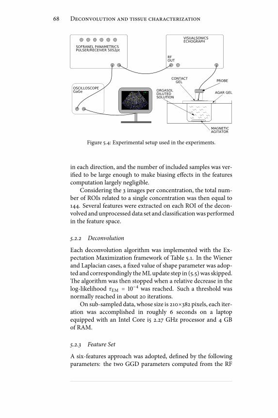
68 Deconvolution and tissue characterization
AGAR GEL
CONTACT GEL
ORGASOLDILUTEDSOLUTION
MAGNETICAGITATOR
SOFRANEL PANAMETRICSPULSER/RECEIVER 5052pt
RFOUT
VISUALSONICSECHOGRAPH
OSCILLOSCOPEGaGe
PROBE
Figure 5.4: Experimental setup used in the experiments.
in each direction, and the number of included samples was ver-ied to be large enough to make biasing eects in the featurescomputation largely negligible.
Considering the 3 images per concentration, the total num-ber of ROIs related to a single concentration was then equal to144. Several features were extracted on each ROI of the decon-volved andunprocessed data set and classicationwas performedin the feature space.
5.2.2 Deconvolution
Each deconvolution algorithm was implemented with the Ex-pectation Maximization framework of Table 5.1. In the Wienerand Laplacian cases, a xed value of shape parameter was adop-ted and correspondingly theMLupdate step in (5.5)was skipped.e algorithm was then stopped when a relative decrease in thelog-likelihood τEM = 10−4 was reached. Such a threshold wasnormally reached in about 20 iterations.
On sub-sampled data, whose size is 210×382 pixels, each iter-ation was accomplished in roughly 6 seconds on a laptopequipped with an Intel Core i5 2.27 GHz processor and 4 GBof RAM.
5.2.3 Feature Set
A six-features approach was adopted, dened by the followingparameters: the two GGD parameters computed from the RF
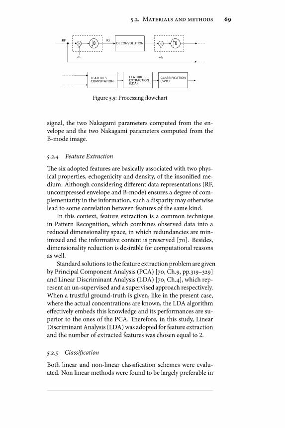
5.2. Materials and methods 69
8
-f0
RF IQDECONVOLUTION 8
+f0
FEATURESCOMPUTATION
FEATUREEXTRACTION(LDA)
CLASSIFICATION(SVM)
Figure 5.5: Processing owchart
signal, the two Nakagami parameters computed from the en-velope and the two Nakagami parameters computed from theB-mode image.
5.2.4 Feature Extraction
e six adopted features are basically associated with two phys-ical properties, echogenicity and density, of the insonied me-dium. Although considering dierent data representations (RF,uncompressed envelope and B-mode) ensures a degree of com-plementarity in the information, such a disparity may otherwiselead to some correlation between features of the same kind.
In this context, feature extraction is a common techniquein Pattern Recognition, which combines observed data into areduced dimensionality space, in which redundancies are min-imized and the informative content is preserved [70]. Besides,dimensionality reduction is desirable for computational reasonsas well.
Standard solutions to the feature extraction problemare givenby Principal Component Analysis (PCA) [70, Ch.9, pp.319–329]and Linear Discriminant Analysis (LDA) [70, Ch.4], which rep-resent an un-supervised and a supervised approach respectively.When a trustful ground-truth is given, like in the present case,where the actual concentrations are known, the LDA algorithmeectively embeds this knowledge and its performances are su-perior to the ones of the PCA. erefore, in this study, LinearDiscriminant Analysis (LDA)was adopted for feature extractionand the number of extracted features was chosen equal to 2.
5.2.5 Classication
Both linear and non-linear classication schemes were evalu-ated. Non linear methods were found to be largely preferable in
70 Deconvolution and tissue characterization
terms of classication errors and computation time, especiallyfor a number of classes higher than 2. In particular, a SupportVector Machine (SVM) with Radial Basis Functions as kernelswas used [70, Ch.5].
Feature extraction and classication partwas performedwiththe Statistical Pattern Recognition Toolbox developed for Mat-lab [71]. A ow chart of the whole processing scheme is reportedin Figure 5.5.
It is worth noting that the main scope of this study was ex-pressively to evaluate the deconvolution contribution to a clas-sication task and not to provide a standard ow for mediumcharacterization through ultrasound. For this reason, the classi-cation scheme proposed in this section might be sub-optimal,but it is nevertheless sucient to give important and trustful in-sights on the eect of a deconvolution step.
5.3 Results
5.3.1 Data classication
Twokind of studiesweremade. In the rst set of trials, four data-sets were separately considered, consisting respectively in theacquired images before and aer deconvolution with the threetechniques, i.e. Wiener ltering, Laplacian prior and the pro-posed scheme. Each data set was then classied with the pro-cessing ow previously described and themisclassication errormeasured.
For each classication task, LDA and SVMwere trainedwith50% of the ROIs, randomly picked from the entire data set. eremaining 50% was adopted as testing set. For any data type,cross-validation was used to nd the optimal kernel parameters,which were then used in the SVM. In order to avoid biasing inthe results due to the specic choice of training and testing sets,20 independent trials were made for each experiment.
In the ideal case, all the concentrations should be simulta-neously discriminated, leading to a seven classes classicationtask. Since classication becomes more challenging as the num-ber of classes increases, several tasks were considered, startingfor the simplest binary case, to the most complicated and com-plete case with 7 classes. e misclassication error was thencomputed: the complete set of results is reported in Table 5.3.
From Table 5.3 several conclusions can be drawn:

5.3.Results
71
Table 5.3: Classication error on 20 independent trials (mean value± standard deviation)
CLASSES CLASSIFICATION ERROR
# CONCENTRATIONS ORIGINAL WIENER LAPLACE GGD
2 [0.5%, 0.75%] 0.1 ± 0.04 0.17 ± 0.04 0.07 ± 0.02 0.001 ± 0.004
3 [0.25%, 6%, 24%] 0.07 ± 0.02 0.03 ± 0.01 0.02 ± 0.01 0.008 ± 0.01
4 [0.75%, 1%, 6%, 24%] 0.20 ± 0.04 0.22 ± 0.02 0.09 ± 0.02 0.02 ± 0.01
5 [0.25%, 0.75%, 1%, 12%, 24%] 0.32 ± 0.02 0.25 ± 0.03 0.08 ± 0.02 0.03 ± 0.01
6 [0.25%, 0.5%, 1%, 6%, 12%, 24%] 0.35 ± 0.02 0.44 ± 0.01 0.11 ± 0.02 0.08 ± 0.01
7 [0.25%, 0.5%, 0.75%, 1%, 6%, 12%, 24%] 0.42 ± 0.02 0.38 ± 0.02 0.19 ± 0.01 0.16 ± 0.01

72 Deconvolution and tissue characterization
−6 −4 −2 0 2 4 6 8
x 10−3
−3
−2
−1
0
1
2
3x 10
−3 ERROR: 0.090278
0.5%0.75%
(a)
−5 −4 −3 −2 −1 0 1 2 3
x 10−3
−3
−2
−1
0
1
2
3
4
5x 10
−3 ERROR: 0
0.5%0.75%
(b)
−0.15 −0.1 −0.05 0 0.05 0.1−0.15
−0.1
−0.05
0
0.05
0.1
0.15
0.2
0.25ERROR: 0.064394
0.25%6%24%
(c)
−0.3 −0.25 −0.2 −0.15 −0.1 −0.05 0 0.05 0.1 0.15−0.1
−0.05
0
0.05
0.1
0.15
0.2
0.25ERROR: 0.0075758
0.25%6%24%
(d)
−0.04 −0.03 −0.02 −0.01 0 0.01 0.02 0.03 0.04−0.015
−0.01
−0.005
0
0.005
0.01ERROR: 0.15179
0.75%1%6%24%
(e)
−0.06 −0.04 −0.02 0 0.02 0.04 0.06 0.08−0.025
−0.02
−0.015
−0.01
−0.005
0
0.005
0.01
0.015
0.02ERROR: 0.020833
0.75%1%6%24%
(f)
−0.2 −0.15 −0.1 −0.05 0 0.05 0.1 0.15 0.2 0.25 0.3−0.15
−0.1
−0.05
0
0.05
0.1ERROR: 0.32598
0.25%0.75%1%12%24%
(g)
−0.4 −0.3 −0.2 −0.1 0 0.1 0.2 0.3−0.08
−0.06
−0.04
−0.02
0
0.02
0.04
0.06
0.08
0.1
0.12ERROR: 0.034314
0.25%0.75%1%12%24%
(h)
Figure 5.6: Scatter plot relative to the testing set before((a),(c),(e),(g)) and aer ((b),(d),(f),(h)) deconvolution with a
GGD prior. e axes correspond to the two features extracted viaLDA. Each row corresponds to a particular number of classes,specically 2, 3, 4 and 5. e black lines correspond to the
boundaries of the classes identied by the SVM.

5.3. Results 73
• Wiener ltering did not bring any contribution to the clas-sication task. Sometimes, even worst results were ob-served with respect to the unprocessed case. is revealsthat Wiener ltering, which is by far the most commonrestoration technique, is not a relevant tool for improv-ing characterization performances. is fact is probablyconnected to the widely documented over-smoothing as-sociated to Wiener ltering [45, 31], in particular whenlow concentrations are considered, where ltering of thepeaky signal components, due to the presence of isolatedscatterers, prevents an eective estimate of their concen-tration.
• Dierently, deconvolutionwith Laplacian priorwas foundto positively aect the classication task. is is particu-larly evident for a high number of classes, where a classi-cation error reduction of up to 20% is associated to thisdeconvolution procedure. Such a behavior is explainedby the fact that a Laplacian model is more eective thanGaussian to provide realistic representations of general re-ectivity structures, in particular when isolated reectorsare superimposed to distributed diusive scattering cen-ters.
• Finally, the proposed deconvolution scheme was found toensure by far the best classication performances. As inthe Laplacian case, the contribution becamemore incisiveas the number of classes increased. In particular, in the4 classes case, the classication error related to the pro-posed framework was still at 2%, while it was four timesbigger for the Laplacian case and ten times for rough data.Moreover, in the most challenging case, in which all con-centrations were simultaneously considered, the classi-cation error was at the satisfactory rate of 16%, while itreached an unacceptable 42% rate on unprocessed data.
In Figure 5.6 several scatter plots are displayed. Each pointrepresents the position of a single ROI of the testing set in theextracted features space; a dierent marker is associated to eachconcentration. Black contours represent the inter-classes bound-aries computed by the SVM classier. From the gure it is evi-dent that classes are better clustered and consequentlymore eas-ily separable aer deconvolution; a much faster and more accu-rate classication is therefore allowed.

74 Deconvolution and tissue characterization
0.8 1 1.2 1.4 1.6 1.8 2 2.2 2.4 2.6 2.80
5
10
15
20
25
30RF SIGNAL
0.5%6%12%24%
(a)
0.8 1 1.2 1.4 1.6 1.8 2 2.2 2.4 2.60
5
10
15
20
25WIENER DECONVOLUTION
0.5%6%12%24%
(b)
0.4 0.5 0.6 0.7 0.8 0.9 1 1.1 1.2 1.30
5
10
15
20
25LAPLACIAN DECONVOLUTION
0.5%6%12%24%
(c)
0.4 0.5 0.6 0.7 0.8 0.9 1 1.1 1.2 1.3 1.40
5
10
15
20
25GGD DECONVOLUTION
0.5%6%12%24%
(d)
Figure 5.7: Generalized Gaussian shape parameter histogramsassociated to four dierent concentrations. In 5.7(a) the
unprocessed case is illustrated. Images 5.7(b), 5.7(c) and 5.7(d)report the situation aer deconvolution is applied, by using Wienerltering, laplacian prior and the proposed method respectively.
As the proposed deconvolution algorithmwas derived in or-der to adaptively restore an estimate of the true reectivity shapeparameter, it was interesting to examine howconcentrationswereseparated accordingly to this parameter only. is is illustratedin Figure 5.7, where a four classes case is observed. When theunprocessed signal is considered, the system PSF eect impliesa mixing of single scatterers contributions, and correspondinglythe density information, explained by the shape parameter, re-sults highly deteriorated. On the contrary, the proposed frame-work allows to retrieve an improved estimate of this importantsignature of the insonied medium. Such a behavior is not en-countered when traditional schemes are applied, which is a di-rect consequence of the biasing eect associated to these meth-ods.
Figure 5.75.7(d) shows clearly how the direct correlation ex-

5.3. Results 75
0.4
0.5
0.6
0.7
0.8
0.9
1
1.1
1.2
1.3
CONCENTRATION
SH
AP
E P
AR
AM
ET
ER
0.5% 6% 12% 24%
Figure 5.8: Boxplot representation of data in Figure 5.75.7(d). Oneach box the central mark is the median and the edges are the 25thand 75th percentiles, the whiskers are the 5th and 95th percentiles.
isting between scatterers concentration and shape parameter isrestored aer deconvolution (see also Figure 5.8).
5.3.2 Feature ranking
Data deconvolved with the proposed algorithm were shown toallow for a more precise characterization. A further study wasthen made to evaluate the eective contribution to the classi-cation task of features computed before and aer deconvolution.
To this purpose, a binary classication task was considered,dened by the two classes corresponding to 0.5% and 0.75% con-centrations. e 6 considered features were then computed onunprocessed and deconvolved data separately, and collected intoan 12 elements feature set. Features were then ranked accord-ing to a distance-based criterion. e total number of classiedsamples in this study was equal to 576; this number derives fromcounting 48 ROIs per image, 3 images per concentration, 2 con-centrations and the fact that unprocessed and deconvolved dataare jointly considered.
In particular, Sequential Forward Selection (SFS) criterionwas used for the ranking [70, Ch.9, pp.315]. SFS is a bottom-up search procedure that adds one feature at a time until thecomplete set is reached. Specically, the feature for which theinter-classes distance J is maximized is added to the feature set

76 Deconvolution and tissue characterization
Table 5.4: Features Ranking
Type Feature Name Signal J1D
D GGD shape RF 3.50
D Nakagami scale Bmode 1.62
D Nakagami shape Bmode 1.26
U Nakagami scale Bmode 0.27
D Nakagami scale envelope 0.95
U Nakagami scale envelope 0.42
U Nakagami shape envelope 0.18
D GGD scale RF 0.73
U GGD scale RF 0.41
U Nakagami shape Bmode 0.44
U GGD shape RF 0.28
D Nakagami shape envelope 0.70
obtained at the previous step, where J was dened in this studyas the Mahalanobis Distance:
J = (µ1 − µ2)T(Σ1 + Σ2)−1(µ1 − µ2) (5.8)
where µ i and Σ i (i ∈ 1, 2) denote the intra class mean valueand covariance matrix respectively.
e nal ranking is reported in Table 5.4, where features aresorted from the rst classied to the last. Features computedaer deconvolution are tagged with a “D” while a tag “U” is as-sociated to unprocessed data. e fourth column visualizes theMahalanobis Distance J1D, corresponding to the selection of asingle-attribute feature set.
From the ranking results provided in Table 5.4 several obser-vations can be made:
• e rst positions in the ranking were occupied by fea-tures computed on deconvolved data. is proves that amore characterizing information on the insonied me-dium can be restored thanks to the proposed deconvo-lution framework. In particular, GGD shape parameterplaced rst in the ranking, which conrms the high sig-nicance of this feature aer deconvolution, cf. Figure 5.7and Figure 5.8;
• If sorting by the value of J1D is made, the rst half of theranking happens to be lled by “D”-tagged features exclu-

5.4. Conclusion 77
sively. at’s to say all features improve their individualdiscrimination capability aer deconvolution.
In order to have more exhaustive evaluation of the decon-volution eect, the same ranking procedure was applied to dif-ferent binary classication tasks. In all those cases, the rst po-sitions in the ranking were systematically occupied by featuresderiving from deconvolved images, which proves the generalityof the latter considerations.
5.4 Conclusion
Ultrasound tissue characterization has become amajor researchsubject. is is motivated by the fact that from the backscatteredecho signal important structural information on the insoniedtissue can be inferred, such as acoustic impedance, scatterer den-sity and distribution pattern. As similar information can dis-criminate between healthy and diseased tissue, this principle canbe exploited within a clinical setting.
As the ultrasound echo suers from the degradation eectdue to the system PSF, deconvolution could be eectively em-ployed as a pre-processing step tomitigate this eect and restoremuch representative information on the true tissue response. Inthis context, this chapter presents a novel deconvolution tech-nique for medical ultrasound, which contains a major concep-tual element of novelty over the existing related literature. In-deed, the goal here is not a mere visual quality improvement,but rather the restoration of a more informative tissue represen-tation, exploitable for an improved characterization.
e performance of the algorithm was evaluated on tissuemimicking phantom studies, which revealed remarkable improve-ments in classication accuracy associated to the implementa-tion of a deconvolution pre-processing step, quantiable in a20%misclassication error reductionwhenmultiple classeswereconsidered. e contribution of other popular deconvolutionschemes was also measured for comparison, and the superiorityof the proposed scheme was correspondingly attested.
When the GGD shape parameter was adopted as the onlyfeature, dierent populations were observed to be clearly sortedby concentration in the feature space (Figure 5.8). is eect wasparticularly evident aer the proposeddeconvolution frameworkwas applied (Figure 5.7). is interesting property could be ex-

78 Deconvolution and tissue characterization
ploited for ultrasound based scatterer concentration sensing andopens the way to further studies in that direction.
Obtained results encourage additional studies on the suit-ability of the proposed algorithm on clinical data. In this sense,few considerations have to be made. At rst, the algorithm ex-ploits a stationarymodel of tissue reectivity, represented by thefact that constant shape parameter and variance are assumed onthe whole image. As a similar assumption is well satised onthe homogeneous phantoms realized for the validation, other-wise it is largely violated on images of biological tissues, wheremultiple tissues with dierent acoustical properties are simul-taneously imaged. In order to deal with these general cases, aparametric image of the shape parameter could tentatively beconsidered instead of a constant value, to be iteratively updatedwithin the optimization ow. Moreover, complementary studieson homogeneous tissue-mimicking phantoms containing poly-disperse suspension of scatterers could be done. is will allowto better mimic situations of clinical interest, like cellular sizevariance during cell death [72], or the simultaneous presence ofglandular acini (100 µm diameter) and cell nuclei (14 µm diam-eter) in breast tumor [73].
A second issue involves the computational complexity. Inthe current, unoptimized Matlab implementation, every frameis processed in roughly two minutes, which is clearly too muchfor assistance during real-time intervention. In this context sub-stantial speed-up could be achieved withmodern GPU comput-ing techniques. In particular, the intrinsic parallelism of the al-gorithm, established by the piecewise constant approximation ofthe PSF, could be eciently handled within GPU architectures,for a fastened execution.

III - Segmentation in Echocardiography

Summary
Cardiovasculardisease (CVD) is themain cause of long-termdisability anddeath for both genderswithin indus-trialized nations. According to theWorld Health Orga-
nization CVD causes over 4 million deaths in Europe and over 2millions in the European Union (EU), corresponding to nearlyhalf of all deaths, cf. Figure B. Besides heavily human, CVD in-volves major economic costs as well. In particular, the overalleconomic cost of CVD has been estimated to be over 192 eurobillions in EU in 2006. ese staggering numbers clearly mo-tivate the intense research activity carried out worldwide dedi-cated to the prevention, early diagnosis and cure of this class ofdiseases.
Modern technology provides a number of tools to accessmy-ocardial function. Echocardiography, in particular, has evolvedas awell-established imaging technique for the noninvasive eval-uation of myocardium abnormalities. Besides the obvious as-pects connected to safety, low cost and portability, echocardi-ography alone oers the possibility of real time observation ofventricular wall motion and deformation, which are fundamen-tal for assessing the extent of possible myocardial ischemia andinfarction. In clinical practice, the analysis mainly relies on vi-sual inspection or manual measurements, o line performed byexperienced cardiologists. Manualmethods are tedious and time-consuming, and visual assessment leads to qualitative and sub-jective diagnoses that suer from considerable inter and intraobserver variability.
e main clinical application concerns the delineation (seg-mentation) and tracking of the myocardium muscle from USscans. Indeed from the position of themuscle boundaries through-out the cardiac cycle several indexes of its function can be in-ferred, as ejection fraction, ventricle volume and wall thickness.For these reasons automating the segmentation of echocardio-
81

82 Summary
Respiratory disease 7%
Other cancer 11%
Lung cancer 6%
Colo−rectal cancer 2%
Stomach cancer 2%
Other CVD 11%
Stroke 11%
Coronary heart disease 21%
All other causes 17%
Injuries and poisoning 12%
(a)
Respiratory disease 6%
Injuries and poisoning 5%
Other cancer 9%
Breast cancer 3%
Lung cancer 2%
Colo−rectal cancer 2%
Stomach cancer 1%
Other CVD 15%
Stroke 17%
Coronary heart disease 22%
All other causes 18%
(b)
Figure B: Deaths by cause for men (a) and women (b) in the lastavailable year in Europe. Data form [74].
graphy images is highly desirable but also challenging. Severalalgorithms have been proposed in literature, documenting suc-cessful results for the detection of the endocardium, i.e. the in-nermost layer of tissue surrounding the ventricular cavity. Oth-erwise, for what concerns epicardial contour, no satisfactory so-lution has been provided yet, in particular when short-axis ac-quisitions are considered. e motivation is that in this kind ofacquisition epicardial bers happen to be collinear with the ul-trasonic beam, and correspondingly the echo returned by these

83
regions is extremely week. e immediate consequence is thatepicardial contours appear highly heterogeneous and discontin-uous on ultrasound frames, which makes their automatic detec-tion particularly challenging.
In this context, we developed a novel semi-automatic frame-work for myocardium segmentation, designed for allowing anecient detection of endo- and epicardial contours of the leventricle in short-axis acquisitions. Level-set technique is adop-ted. Statistics of the echo signal along with geometrical consid-erations on the myocardium expected shape are originally ex-ploited for constraining the curve motion towards anatomicallymeaningful shapes. A localizing strategy recently proposed inliterature was adopted, ensuring robustness against low contrastand missing contours.
is project has been developed during a one year intern-ship within the ultrasound equipe of the Centre de recherche enimagerie médicale (CREATIS-LRMN) of Lyon - France, underthe supervision of Prof. Olivier Bernard and Prof. Olivier Bas-set. is work has resulted in 4 publications up to the presenttime [75, 76, 77, 78]. Due to their general formulation, the de-veloped tools have proved their suitability for amuchwider classof images which exceeds medical ultrasound [76, 78].
is part of the thesis is structured as follows: in Chapter 6the reader is supplied with the necessary theoretical backgroundon level-set segmentation. Starting from standard region-basedapproaches, general ways for including localization and shapeinformation are presented as well. In Chapter 7 the basics ofheart morphology and functioning are described. In Chapter 8the proposed segmentation framework is described and a vali-dation on clinical data is presented.


Chapter 6Level-set segmentation
From the pioneering work of Kass et al.[79], variationaltechniques have beenwidely exploited for image segmen-tation purposes. Due to their extreme generality andex-
ibility, these methods can be suitably specialized in order to dealwith data of the most general nature: medical, biological and as-tronomical are some examples. In synthesis, active contours seg-mentation consists in the displacement of a curve on the imageplane. is motion pursues the attachment to the boundaries ofthe interesting target and is normally governed by theminimiza-tion of an a priori dened cost functional. An elegant and e-cient formalization of active contours segmentation is providedby level-sets [80, 81], which are the object of this chapter. e in-terested reader may nd almost exhaustive reviews on level-setsin [19, 82].
e rest of the chapter is structured as follows. In §6.1 thegeneral level-set formalism is introduced. In §6.2 the standardregion-based approach is illustrated, while in §6.3 amore recent,localized solution is discussed. In §6.4 and §6.5 it is shown howstatistical and geometrical information can be exploited in thesegmentation process. In §6.6 some concluding considerationsare made.
6.1 General
Let I ∶ Ω → Rm be a given image, where Ω ⊂ R
d and m is thecardinality of the feature space in which the image exists. Forinstance ism = 1 for gray-scale data and m = 3 for colored ones.In the level-set formalism, the evolving interface Γ ⊂ Ω is rep-
85
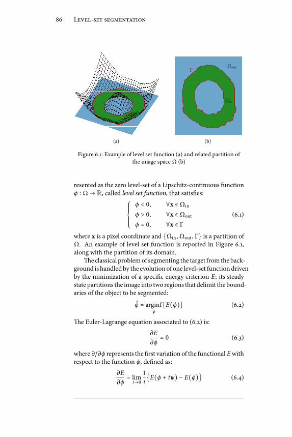
86 Level-set segmentation
(a)
Ωin
Ωout
Γ
(b)
Figure 6.1: Example of level set function (a) and related partition ofthe image space Ω (b)
resented as the zero level-set of a Lipschitz-continuous functionϕ ∶ Ω → R, called level set function, that satises:⎧⎪⎪⎪⎪⎨⎪⎪⎪⎪⎩
ϕ < 0, ∀x ∈ Ωin
ϕ > 0, ∀x ∈ Ωout (6.1)
ϕ = 0, ∀x ∈ Γwhere x is a pixel coordinate and Ωin , Ωout , Γ is a partition ofΩ. An example of level set function is reported in Figure 6.1,along with the partition of its domain.
e classical problemof segmenting the target from the back-ground is handled by the evolution of one level-set functiondrivenby the minimization of a specic energy criterion E; its steadystate partitions the image into two regions that delimit the bound-aries of the object to be segmented:
ϕ = arginfϕ
E(ϕ) (6.2)
e Euler-Lagrange equation associated to (6.2) is:
∂E
∂ϕ= 0 (6.3)
where ∂/∂ϕ represents the rst variation of the functional Ewithrespect to the function ϕ, dened as:
∂E
∂ϕ= lim
t→0
1
tE(ϕ + tψ) − E(ϕ) (6.4)
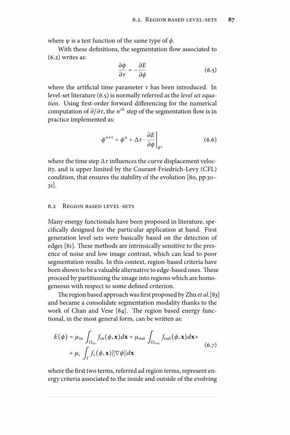
6.2. Region based level-sets 87
where ψ is a test function of the same type of ϕ.With these denitions, the segmentation ow associated to
(6.2) writes as:∂ϕ
∂τ= −∂E
∂ϕ(6.5)
where the articial time parameter τ has been introduced. Inlevel-set literature (6.5) is normally referred as the level set equa-tion. Using rst-order forward dierencing for the numericalcomputation of ∂/∂τ, the nth step of the segmentation ow is inpractice implemented as:
ϕn+1 = ϕn + ∆τ ⋅∂E
∂ϕ∣ϕn
(6.6)
where the time step ∆τ inuences the curve displacement veloc-ity, and is upper limited by the Courant-Friedrich-Levy (CFL)condition, that ensures the stability of the evolution [80, pp.30–31].
6.2 Region based level-sets
Many energy functionals have been proposed in literature, spe-cically designed for the particular application at hand. Firstgeneration level sets were basically based on the detection ofedges [81]. ese methods are intrinsically sensitive to the pres-ence of noise and low image contrast, which can lead to poorsegmentation results. In this context, region-based criteria havebeen shown to be a valuable alternative to edge-based ones. eseproceed by partitioning the image into regions which are homo-geneous with respect to some dened criterion.
e region based approachwas rst proposed byZhu et al.[83]and became a consolidate segmentation modality thanks to thework of Chan and Vese [84]. e region based energy func-tional, in the most general form, can be written as:
E(ϕ) = µin ∫Ωin
fin(ϕ, x)dx + µout ∫Ωout
fout(ϕ, x)dx++ µc ∫
Γfc(ϕ, x)∣∣∇ϕ∣∣dx (6.7)
where the rst two terms, referred ad region terms, represent en-ergy criteria associated to the inside and outside of the evolving

88 Level-set segmentation
contour, while the third one, called contour term, is associatedto the interface Γ. By introducing the Heaviside step function
H(x) = ⎧⎪⎪⎨⎪⎪⎩1, if x ≥ 00, if x < 0 . (6.8)
and the Dirac delta function δ(⋅), (6.7) becomes:
E(ϕ) = µin ∫Ωfin(ϕ, x)H(−ϕ)dx+
+ µout ∫Ωfout(ϕ, x)H(ϕ)dx+
+ µc ∫Ωfc(ϕ, x)∣∣∇ϕ∣∣δ(ϕ)dx.
(6.9)
Let’s note that, in order to compute the Euler-Lagrange equa-tion, a regularized version of H and δ must be considered. Apossible choice is given by [17]:
Hτ(x) = 1
2(1 + 2
πarctan(x
τ))
δτ(x) = d
dxHτ(x) = 1
π⋅
R
τ2 + x2
(6.10)
where τ ≪ 1 is the regularizing constant.It is common to adopt the contour force fc(⋅, ⋅) constantly
equal to 1 [84]. With this substitution, the related energy termbecomes ameasure of the curve length and imposes a constrainton the regularity of its shape. e rst variation of the corre-sponding contour term, referred as Ec, is expressed by:
∂Ec
∂ϕ= δ(ϕ) ⋅ κ, κ = ∇ ⋅ ( ∇ϕ∣∇ϕ∣ ) (6.11)
where κ is the curvature of the interface [80, Chapter 1]. In stan-dard level-set segmentation techniques this term is commonlyintroduced to preserve the stability of the evolution, and the cor-responding weight µc is tuned so to obtain a contour of the de-sired smoothness.
6.2.1 Example: Chan-Vese functional
e framework introduced by Chan and Vese [84] fairly repre-sents the most commonly adopted level set strategy, at least at

6.3. Localized level sets 89
(a) (b)
Figure 6.2: Result of Chan-Vese algorithm on images withhomogeneous (a) and heterogeneous intensity proles (b).
a rst attempt. is popular criterion will be adopted in the se-quel in order to illustrate the developed concepts and is brieydescribed in this section.
e proposed energy function writes as:
E = ∫Ω∣I(x) − cin∣2H(−ϕ)dx+
+∫Ω∣I(x) − cout ∣2H(ϕ)dx+
+ µ∫Ω∣∣∇ϕ∣∣δ(ϕ)dx
(6.12)
which leads to the evolution law:
∂ϕ
∂τ= δ(ϕ) [−∣I(x) − cin∣2 + ∣I(x) − cout∣2 + µ∇ ⋅ ( ∇ϕ∣∇ϕ∣ )]
where cin and cout represent the mean values of pixel intensityI(x) measured inside and outside of the evolving contour re-spectively. Correspondingly, the functional in (6.12) partitionsthe image into regions which are maximally homogeneous withrespect to the average intensity.
6.3 Localized level sets
Region-based approaches present several advantageswith respectto edge-based ones, including robustness against initial curveplacement and insensitivity to noise. However, these techniquesare derived on the base of a strong hypothesis, consisting in thefact that regions of interest can be dierentiated in terms of their

90 Level-set segmentation
Ωin
Ωout
(a)
Ωout,x
Ωin,x
x
(b)
Figure 6.3: Dierence between region-based and localizedapproach. In the rst case (a) the whole image content is used forinterface evolution, in the second case (b) a smaller sub-image is
considered instead.
global statistics. In many practical situations, the object to besegmented may be occluded, or its intensity proles may be het-erogeneous, for instance due to spatial variations in the illumi-nation. In these situations traditional region based algorithmsmay return erroneous segmentation results, see Figure 6.2.
To accurately segment these objects, a new class of activecontours energies has been presented in [85], which utilizes lo-cal information instead of global one. e initiative is that, if thehomogeneity hypothesis is not satised globally, there’s a greaterprobability for it to be satised within smaller sub-regions. Cor-respondingly, a variational formulation is derived, which gener-alizes the region-based formalism by including such a localizingprinciple. is is realized by the binary mask:
W(x, y) = ⎧⎪⎪⎨⎪⎪⎩1, if ∣x − y∣ < ρ0, otherwise
(6.13)
selecting the local regions (spheres of radius ρ in this case) inwhich the driving force is computed. In (6.13) x and y representthe coordinates of two points in Ω. e localized energy func-tion, in its most general form, writes as:
E(ϕ) =∫Ωδ(ϕ(x))∫
ΩW(x, y)F(I(y), ϕ(y))dy dx+
+ µ∫Ωδ(ϕ)∣∣∇ϕ∣∣dx
(6.14)
6.3. Localized level sets 91
(a) (b)
Figure 6.4: Standard region-based Chan-Vese (a), localizedChan-Vese (b).
where F is a generic internal energy measure, used to representlocal adherence to a given model at each point along the con-tour. A visual representation of the localizing approach is givenin Figure 6.3. Instead of considering the entire image, curve ve-locity is computed in the local subsets Ωin,x and Ωout,x, denedas:
Ωin,x = x∣ϕ(x) < 0, x ∈ N(x)Ωout,x = x∣ϕ(x) > 0, x ∈ N(x) (6.15)
where N(x) = y∣W(x, y) = 1.e level set equation then is derived as:
∂ϕ
∂τ=δ(ϕ(x))∫
ΩW(x, y)∇ϕF(I(y), ϕ(y))dy+
+ µ∇ ⋅ ( ∇ϕ∣∇ϕ∣ )(6.16)
Equation (6.16) provides a simple way to convert virtuallyevery region-based criterion to its localized equivalent. In Fig-ure 6.4 a comparison is presented between the tradition Chan-Vese scheme and its localized version. Due to the presence of anheterogeneous illumination and poorly contrasted boundariesthe global approach does not succeed in producing a correctsegmentation, which is obtained when the localized version isemployed instead.
is important capability provided by localized schemes willbe protably exploited in the design of a le-ventricle segmenta-tion algorithm. Indeed, due to the complex interactions between

92 Level-set segmentation
the tissue and the ultrasonic beam, le ventricle contours appearhighly discontinuous and heterogeneous in the image. Localizedlevel sets represent therefore a powerful candidate to deal withthese problematic image characteristics.
6.4 Statistical level sets
e extremely general level sets formalism allows to embed sev-eral sources of information in the segmentation process. Signalstatistics, textures, colors, expected target shape are examples,see [86] for a review.
In the context of ultrasound images,methods based on specklestatistics are commonly developed, indeed in such images thehigh noise makes standard approaches based on intensity pro-les and edges unusable. Hereto, the focus of this section will beon statistically inspired level-set segmentation. Two approachesare reviewed, the rst,more common,Maximum-likelihood (ML)criterion by Sarti et al.[17], along with a more recent one, basedon the Bhattacharyya distance by Michailovich et al.[87].
6.4.1 Maximum Likelihood Segmentation
Let I be the image to be segmented and Γ the segmenting con-tour, the ML criterion seeks the contour which maximizes thea-posteriori probability P(I∣Γ) [88]. In a level set formalism thisis equivalent to nding the level set function ϕ maximizing:
E(ϕ) = P(I∣ϕ) = Pin(I∣ϕ) ⋅ Pout(I∣ϕ) (6.17)
where statistical independence between the regions dened byΩin and Ωout has been assumed. Assuming as well indepen-dence of the pixels within each region, then it is:
Pin = ∏x∈Ωin
pin(I(x)), Pout = ∏x∈Ωout
pout(I(x)), (6.18)
where pin(⋅) and pout(⋅) represent the probability density func-tion (pdf) associated to the pixel intensity I in the inside andoutside regions.
Due to the complexity related to the product operations, itis common to maximize the logarithm of (6.17) instead of (6.17)itself. Since the logarithm function is monotonically increasingthese two operations are indeed equivalent. By making use of

6.5. Shape prior constraints 93
the Heaviside step function, then the energy function becomes:
E(ϕ) =∫Ωlog pin(I)H(−ϕ)dx+
∫Ωlog pout(I)H(ϕ)dx. (6.19)
In [17] a ML framework is presented for the segmentationof medical ultrasound images. In that work a standard Rayleighdistribution is adopted for the uncompressed envelope signal.Interesting results are reported in echocardiography and obstet-rics.
6.4.2 Bhattacharyya Distance Segmentation
In [87] a level-set segmentation criterion is proposed based onthe notion of statistical distance. Specically, it proceeds by par-titioning the image into regionwhich aremaximally distant withrespect to the given metric. In particular the Bhattacharyya dis-tance is there adopted. Given two pdfs pin and pout, this is de-ned as D = − logB, where:
B(pin∣pout) = ∫R
√pin(I)pout(I)dI (6.20)
is the Bhattacharyya coecient. In particular, the segmentationow in [87] is driven by theminimization of B, which, due to theto fact that the logarithm function is monotonically increasing,is perfectly equivalentmaximization ofD. is avoids computa-tional issues associated to the evaluation of the logarithm func-tion. Non parametric kernel-based estimates of the two pdfs areused in [87], which makes the algorithm independent on anyprior assumption on the intensity distribution.
According to the authors, their framework presents compu-tational advantages over the ML one. is is motivated by thefact that the logarithm function used in (6.19) is known to bevery sensitive to variations of its argument in vicinity of rela-tively small values of the latter.
6.5 Shape prior constraints
It has been shown how level sets provide suitable tools for ad-dressing extremely general segmentation tasks, allowing to eas-ily embed several kind of image information, like intensity, edges,

94 Level-set segmentation
texture, color and many others. In many practical cases occlu-sions, low contrast or low SNR make image data insucient forproducing meaningful results. In these cases higher-level priorknowledge about the shape of the expected object, if available,can be exploited in the segmentation process, see e.g. [89, 90, 91,86, 92].
In level-set literature, the shape information is oen takeninto account by considering the linear combination of two terms[89, 90]. e rst one, referred as data attachment term, drivesthe segmentation to particular image features. e second, re-ferred as shape prior term, preserves the similarity between themoving interface and a reference shapemodel. e choice of theprior model is a fundamental issue: typically it is derived fromthe statistical analysis of a set of training examples [89, 90, 93].Since orientation and scale of the target are a priori unknown,a transformation is performed at each iteration to align the seg-mented contour with the prior shape. is step is mainly ad-dressed in a steepest descent framework [90, 89].
Let’s denote data attachment and shape prior terms as Edata
and Eshape respectively. Here Edata can be any of the energy cri-terion previously introduced. e global energy function thenwrites as:
E(ϕ, λ) = Edata(ϕ) + α ⋅ Eshape(ϕ, λ) (6.21)
where α corresponds to a positive hyper-parameter that balancesthe inuence between the two terms, and λ represents the pa-rameters of the adopted model (for instance, λ could denotescale, position and orientation of the reference shape [90]). eshape prior term is commonly implemented as a distance mea-sure between the active contour and the expected shape, and itseect is to penalize those solutions which are not consistent withthe model itself.
Shape prior segmentation is then dened as:
(ϕ, λ) = argminϕ ,λE(ϕ, λ) (6.22)
which can be solved iteratively with the two step scheme:
ϕn+1 = ϕn + ∆τ ⋅∂E
∂ϕ∣(ϕn ,λn)
(6.23)
λn+1 = argmin
λ
Eshape(ϕn+1 , λ) (6.24)

6.6. Conclusion 95
erst operation corresponds to the displacement of the activecontour, while the second step seeks the ane transformationmapping the prior shape onto the active contour itself. For arbi-trary shapes Eshape must be computed numerically and the cor-responding optimization (6.24)must be solved iteratively,mainlywith steepest descent schemes [90]. In these situations the com-putational burden associated to the shape priormay become con-siderable.
6.6 Conclusion
In this chapter the basic elements of level-set theory have beenprovided. Traditional region based schemes have beendescribedin §6.2, with some detail on the renown Chan-Vese functional,which represents the pioneering work in this eld. e recentframework by Lankton et al.has been presented in §6.3, whichimproves robustness against heterogeneous or missing bound-aries by introducing a localization concept. Since edges and in-tensity proles are not a trustful source of information in highlynoisy situations, a common way to deal with these data is to ex-ploit noise statistics within the segmentation ow. Hereto, in§6.4 two dierent approaches have been reviewed, based on theconcepts of Maximum likelihood estimation and statistical dis-tance. Finally, §6.5 has been dedicated to the formalization of theshape prior segmentation framework. Guesses on the expectedshape of the desired target are extremely useful when image dataare not sucient for an accurate segmentation, like in the caseof occlusions, low contrast or low SNR.


Chapter 7Myocardium anatomy and functioning
The heart is one of the most vital organs in the humanbody. It is located between the lungs in the middle ofthe chest, behind and slightly to the le of the breast-
bone (sternum). Its fundamental role consists in preserving theactivity of the circulatory systems by pumping blood throughthe entire human body. In particular it cyclically receives de-oxygenated blood and pumps it to the lungs to enrich it withfresh oxygen.
In this chapter the basics of heart anatomy and functioningare described in §7.1 and §7.2. In §7.3 an emphasis is put on thele ventricular chamber, which exploits the most onerous me-chanical eort in the heart cycle and is the region maximallysubject to possible diseases. e importance of le ventricle seg-mentation as a diagnostic tool to observe and quantify heart de-ciencies is then stressed in §7.4, where a literature overview ofle ventricle segmentation algorithms is presented. In §7.5 someconclusions are drawn.
7.1 Heart anatomy
e heart is the muscular organ responsible for pumping oxy-genated blood throughout the vessels by repeated, rhythmic con-tractions. It is composed of an involuntary striated muscle tis-sue, calledmyocardium. e innermost and outermost layers oftissues are called endocardium and epicardium respectively. eendocardium ismanlymade of epithelial and connective tissues.It lines the inner cavities of the heart, covers heart valves and iscontinuous with the inner lining of blood vessels, moreover it
97

98 Myocardium anatomy and functioning
Figure 7.1: Anatomy and functioning of human heart muscle.http://www.childrenshospital.org/az/Site509/Images/normal_large.gif
hosts the Purkinje bers, which participate in the contractionof the heart muscle. Dierently, the epicardium is mainly con-stituted of connective tissue and functions as a protective layer.e heart muscle is contained within a sac called pericardium,which is attached to the central part of the diaphragm and theback of the breastbone. e pericardium is lledwith pericardialuid, which acts as a lubricant to allow normal heart movementwithin the chest.
e heart is composed of four chambers: the two upper atria(singular atrium) and the two lower ventricles. Le ventricle isseparated from the right one by the ventricular septum, while leatrium is separated from the right one by the atrial septum. Inan healthy heart blood ow is unidirectional, the actual path isindicated in Figure 7.1 by means of white arrows. is is madepossible by a system of valves. In particular, the right atriumcommunicates with the right ventricle by means of the tricuspidvalve, while themitral valve links le atrium to the le ventricle.e aortic valve connects the le ventricle to the aorta, the ma-jor artery of the human circulatory system, while the pulmonaryvalve connects the right ventricle to the pulmonary artery, cf.Figure 7.1.

7.2. Heart functioning 99
7.2 Heart functioning
e cardiac muscle acts fundamentally as a pump: blood is re-ceived by the atria, moved to the ventricles, and then returned tothe circulatory system. Blood ow within the heart is regulatedby coordinated contractions (systole) and relaxations (diastole)of the four chambers. In particular both atria contract simulta-neously as the ventricles are relaxed and vice versa. is allowsblood to ow from the atria into the ventricles, and then againinto the circulatory system. Reuxes are prevented by the ac-tion of the valves. Valves functioning is purely mechanical: theyopen when gradient of blood pressure has a certain sign, andclose when the opposite situation happens.
A schematic of heart functioning is illustrated in Figure 7.1.Oxygen-depleted blood is received in the right atrium from thesuperior vena cava during atrial diastole. en right atrium con-tracts and blood ows through the tricuspid into the right ven-tricle. During ventricular systole the tricuspid closes and bloodin the right ventricle is pumped into the pulmonary artery andthen to the lungs, where it is oxygenated. Oxigenated bloodows into the le half of the heart: form the le atrium to thele ventricle, and then into the aorta. e portion of the cir-culatory system which starts in the aorta and ends in the venacava is called systemic circulation, and distributes oxygen andnutrients to the entire body. e portion which starts in thepulmonary artery, passes through the lungs, and ends in the pul-monary veins, is called pulmonary circulation, and is responsiblefor blood re-oxygenation.
is operation is repeated cyclically and is referred as car-diac cycle. In an adult healthy heart, it repeats with a frequencyof roughly 72 beats per minute (bpm). e sequence of contrac-tions and relaxations is regulated by the propagation of electricpulses, released periodically by the sinoatrial node, or peace-maker, located in the right atrium.
7.3 Left ventricle
e le ventricle is the heart chamber to which the most in-tense mechanical eort is demanded, indeed it is responsible forpumping blood throughout the entire human body. For this rea-son the large majority of cardiopathies aect this region.
Eciency of the le ventricle is mainly evaluated by mea-suring its capability to feed the human physic with satisfactory
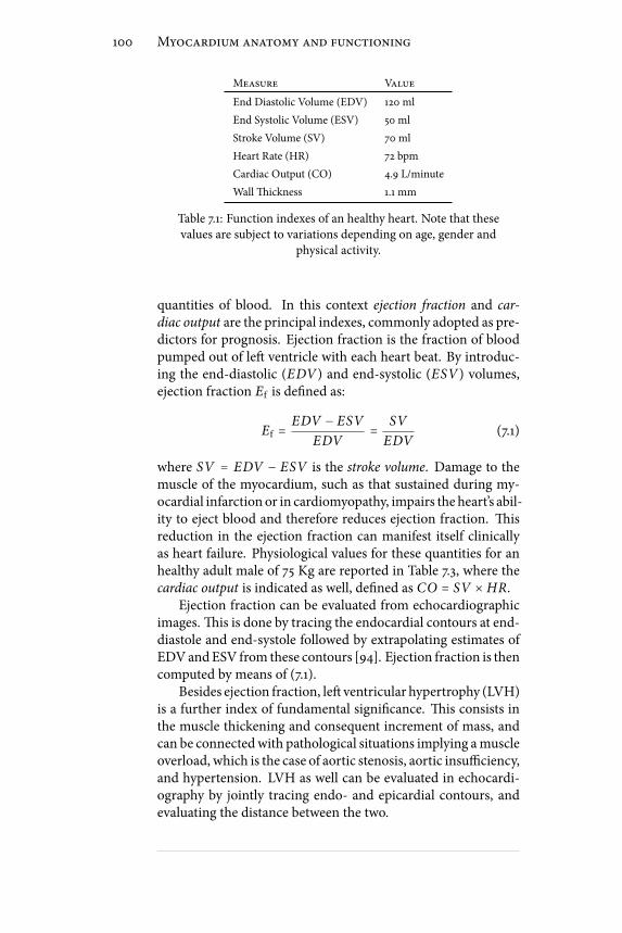
100 Myocardium anatomy and functioning
Measure Value
End Diastolic Volume (EDV) 120 ml
End Systolic Volume (ESV) 50 ml
Stroke Volume (SV) 70 ml
Heart Rate (HR) 72 bpm
Cardiac Output (CO) 4.9 L/minute
Wallickness 1.1 mm
Table 7.1: Function indexes of an healthy heart. Note that thesevalues are subject to variations depending on age, gender and
physical activity.
quantities of blood. In this context ejection fraction and car-diac output are the principal indexes, commonly adopted as pre-dictors for prognosis. Ejection fraction is the fraction of bloodpumped out of le ventricle with each heart beat. By introduc-ing the end-diastolic (EDV ) and end-systolic (ESV ) volumes,ejection fraction Ef is dened as:
Ef = EDV − ESVEDV
= SV
EDV(7.1)
where SV = EDV − ESV is the stroke volume. Damage to themuscle of the myocardium, such as that sustained during my-ocardial infarction or in cardiomyopathy, impairs the heart’s abil-ity to eject blood and therefore reduces ejection fraction. isreduction in the ejection fraction can manifest itself clinicallyas heart failure. Physiological values for these quantities for anhealthy adult male of 75 Kg are reported in Table 7.3, where thecardiac output is indicated as well, dened as CO = SV ×HR.
Ejection fraction can be evaluated from echocardiographicimages. is is done by tracing the endocardial contours at end-diastole and end-systole followed by extrapolating estimates ofEDVandESV from these contours [94]. Ejection fraction is thencomputed by means of (7.1).
Besides ejection fraction, le ventricular hypertrophy (LVH)is a further index of fundamental signicance. is consists inthe muscle thickening and consequent increment of mass, andcan be connectedwith pathological situations implying amuscleoverload, which is the case of aortic stenosis, aortic insuciency,and hypertension. LVH as well can be evaluated in echocardi-ography by jointly tracing endo- and epicardial contours, andevaluating the distance between the two.
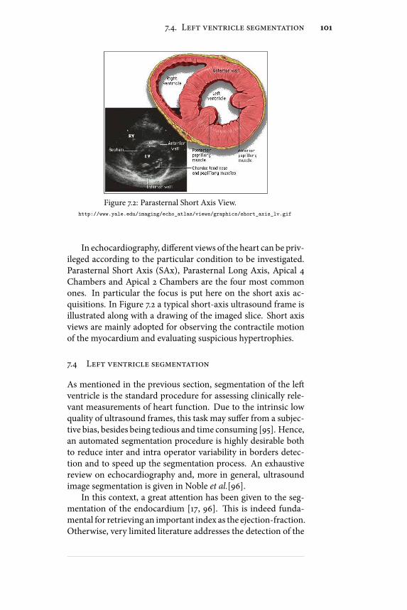
7.4. Left ventricle segmentation 101
Figure 7.2: Parasternal Short Axis View.http://www.yale.edu/imaging/echo_atlas/views/graphics/short_axis_lv.gif
In echocardiography, dierent views of the heart can be priv-ileged according to the particular condition to be investigated.Parasternal Short Axis (SAx), Parasternal Long Axis, Apical 4Chambers and Apical 2 Chambers are the four most commonones. In particular the focus is put here on the short axis ac-quisitions. In Figure 7.2 a typical short-axis ultrasound frame isillustrated along with a drawing of the imaged slice. Short axisviews are mainly adopted for observing the contractile motionof the myocardium and evaluating suspicious hypertrophies.
7.4 Left ventricle segmentation
As mentioned in the previous section, segmentation of the leventricle is the standard procedure for assessing clinically rele-vant measurements of heart function. Due to the intrinsic lowquality of ultrasound frames, this task may suer from a subjec-tive bias, besides being tedious and time consuming [95]. Hence,an automated segmentation procedure is highly desirable bothto reduce inter and intra operator variability in borders detec-tion and to speed up the segmentation process. An exhaustivereview on echocardiography and, more in general, ultrasoundimage segmentation is given in Noble et al.[96].
In this context, a great attention has been given to the seg-mentation of the endocardium [17, 96]. is is indeed funda-mental for retrieving an important index as the ejection-fraction.Otherwise, very limited literature addresses the detection of the

102 Myocardium anatomy and functioning
epicardium. e motivation is that in this kind of acquisitionsepicardial bers happen to be collinear with the ultrasonic beamand the echo returned by these regions is extremely week, withthe immediate consequence that epicardial contours appear highlyheterogeneous and discontinuous on the resulting image, anddicult to be detected automatically. Nevertheless a trustful de-tection of both boundaries has a high clinical relevance, sinceit would allow the computation of fundamental parameters asthe ventricular mass, which has been proven to be an impor-tant precursor for a variety of conditions such as cardiomyopa-thy, hypertension and valvular disease [97]. Among the very fewworks addressing the segmentation of the whole myocardiumfrom SAx acquisitions, the most popular ones are [98, 99, 100].
In [98] Dias et al.proposed an algorithm searching for endoand epicardial contours along privileged radial directions start-ing from a guess of myocardium center. e estimation problemwas modeled in a Bayesian framework as a maximum a posteri-ori estimation problem with Rayleigh statistics for the data termand a spatio-temporal Markov Random Field for the regulariza-tion term. An iterative multigrid dynamic programming algo-rithm was used to solve the optimization problem.
In [99] Chalana et al.developed a multiple active contourmethod for segmentation of 2D+T sequences. ey used theimage intensity gradient as the attracting force and invoked tem-poral continuity via an external energy term that constrainedthemotion between consecutive frames. e dierent contribu-tions to the curve evolution were balanced according to a set of14 empirically set parameters. e algorithmwas initializedwitha manual delineation of the epicardium and the epicardium wascorrespondingly searched in an automatic way. e two con-tours were then segmented in sequence throughout the entireacquisition.
In [100] Setarehdan et al.developed a fuzzy multiscale edgedetection (FMED) method that uses a wavelet transform to de-ne the various levels of resolution of image content. In thiswork, an edge was dened as a point with maximal member-ship of the edge fuzzy set. Temporal information was includedin edge detection by dening a moving edge fuzzy membershipfunction, as well as an edge fuzzy membership function. ecombined edge andmotionmembership functionwas thenmax-imized to dene edge points.
In this scenario we propose a novel algorithm for combinedsegmentation of endo and epicardium from SAx acquisitions

7.5. Conclusion 103
which is believed to overcome several shortcomings associatedwith existing methods. In particular:
• Results of [99] rely on empirically tuning a set of 14 pa-rameters, which highly reduces the clinical usability of thesegmentation tool. On the contrary, the proposed algo-rithm requires 3 parameters only to be set, all with a veryspecicmeaning. As a consequence they can be intuitivelyadjusted by the user in order to obtain the best results.
• In [99] and [100] image gradient is adopted as edge indi-cator employed for location of endo and epicardium. Itis well established that image gradient alone is not a reli-able source of information for heavily speckle corruptedimages as ultrasound ones are. For similar data, to em-ploy speckle statistics as driving criterion has become theconsolidated practice instead. In particular, in the pro-posed algorithm a Rayleigh distribution is assumed forthe speckle and myocardium is segmented by nding themaximum statistical separation from the background.
• e work in [98] formalizes the segmentation problem asthe optimization of a non convex cost function, which issolved by a computationally cumbersome and hardly im-plementable multigrid dynamic programming algorithm.Since the advent of level sets, they became one of themostpopular alternatives for formalizing segmentation prob-lems, indeed they allow both simple and ecient imple-mentation. For this reasonwe formalize our segmentationproblem on the base of the level set theory.
A complete description of the proposed algorithm will beaddressed in the next chapter.
7.5 Conclusion
In this chapter the basis of heart morphology and functioninghave been provided and several indexes of cardiac function havebeen presented. e importance of le ventricle segmentationfor assessing those performance metrics has been justied andseveral algorithms addressing this task in an automatic or semi-automatic way have been briey reviewed. In such a scenariothe proposed myocardium segmentation tool has been contex-tualized. is will be the subject of the next chapter, where anevaluation on clinical data will be presented.


Chapter 8Myocardium segmentation
In this chapterwe present an original semi-automatic toolfor combined segmentation of endo- and epicardium in 2Dechocardiography. e algorithm is based on the level set
theory and exploits all the concepts of localization, statisticalsegmentation and shape priors introduced in Chapter 6.
e rest of the chapter is structured as follows. In §8.1 werecall the general form of the shape prior level-set framework,describe our shape prior term and derive the minimization ofthe corresponding energy functional. A strategy for preventingcollisions between the two contours is described as well. In §8.2,implementation issues are addressed. We explain in particularhow the level-set is initialized for each experiment. e exper-imental setup and the adopted performance metrics are illus-trated in §8.3 and §8.4 respectively. In §8.5 we then provide anevaluation of the method on cardiac images. ough the mainemphasis will be put on US images a validation on natural im-ages andMRI will be presented as well in §8.6, showing the ex-ibility of the framework. e main conclusions of this work aregiven in §8.7.
8.1 Proposed segmentation framework
Many energy functionals have been proposed in literature to in-corporate shape priors into level-set formulation. As in [93, 89,86] we adopt the general expression for the energy function of(6.21), reported here for the sake of completeness:
E(ϕ, λ) = Edata(ϕ) + α ⋅ Eshape(ϕ, λ) (8.1)
105
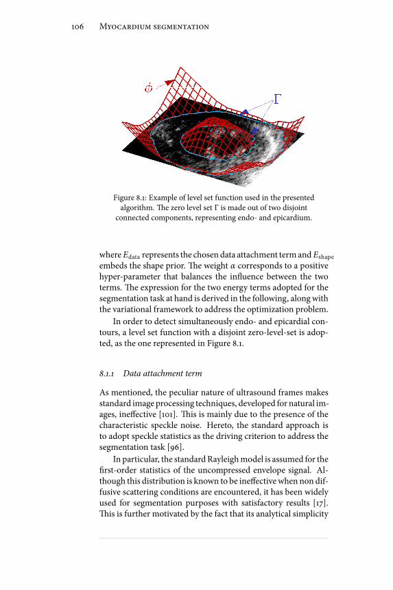
106 Myocardium segmentation
Figure 8.1: Example of level set function used in the presentedalgorithm. e zero level set Γ is made out of two disjoint
connected components, representing endo- and epicardium.
where Edata represents the chosendata attachment termand Eshape
embeds the shape prior. e weight α corresponds to a positivehyper-parameter that balances the inuence between the twoterms. e expression for the two energy terms adopted for thesegmentation task at hand is derived in the following, alongwiththe variational framework to address the optimization problem.
In order to detect simultaneously endo- and epicardial con-tours, a level set function with a disjoint zero-level-set is adop-ted, as the one represented in Figure 8.1.
8.1.1 Data attachment term
As mentioned, the peculiar nature of ultrasound frames makesstandard image processing techniques, developed for natural im-ages, ineective [101]. is is mainly due to the presence of thecharacteristic speckle noise. Hereto, the standard approach isto adopt speckle statistics as the driving criterion to address thesegmentation task [96].
In particular, the standardRayleighmodel is assumed for therst-order statistics of the uncompressed envelope signal. Al-though this distribution is known to be ineectivewhen non dif-fusive scattering conditions are encountered, it has been widelyused for segmentation purposes with satisfactory results [17].is is further motivated by the fact that its analytical simplicity

8.1. Proposed segmentation framework 107
allows the closed form solution for the integrals involved in thesegmentation ow, which is desirable for a fast computation.
e Bhattacharyya coecient (6.20) is adopted as data at-tachment term Edata. By embedding the Rayleighmodel the twodiscriminating distributions write as:
pin(I) = I
σ 2in
exp− 1
2σ 2in
, pout(I) = I
σ 2out
exp− 1
2σ 2out
(8.2)
where σin and σout represent the Rayleigh parameter estimatedinside and outside of the moving interface. In the context oflevel-sets, this parameter can be estimated in a ML sense insideand outside the evolving interface from the following two ex-pressions:
⎧⎪⎪⎪⎪⎪⎪⎪⎨⎪⎪⎪⎪⎪⎪⎪⎩
σ 2in(ϕ) = 1
2⋅ ∫Ω I2(x)H(−ϕ(x))dx∫ΩH(−ϕ(x))dx
σ 2out(ϕ) = 1
2⋅ ∫Ω I2(x)H(ϕ(x))dx∫ΩH(ϕ(x))dx
(8.3)
By substituting the Rayleighmodel into the expression of theBhattacharyya coecient, it becomes:
BR(ϕ) = 2 ⋅ σin(ϕ) ⋅ σout(ϕ)σ 2in(ϕ) + σ 2
out(ϕ) (8.4)
with σin and σout dened as in (8.3).While region-based active contours have been successfully
used for endocardium segmentation [17], they result otherwiseineective in providing meaningful segmentations of the epi-cardium. is is due to the fact that, when a short axis acquisi-tion is made, myocardial bers and the ultrasonic beam happento be collinear at the epicardium. Correspondingly, it returns anextremely weak echo and its boundaries appear poorly denedin the image and are therefore dicult to be located in an auto-matic way. It was shown in the Chapter 6 that a localizing ap-proach can be exploited in order to deal with similar problematicimage features. Hereto a localized version of the Bhattacharyyadistance is adopted.
e localized energy then writes as [75]:
BR ,x(ϕ) = 2 ⋅ σin,x(ϕ) ⋅ σout,x(ϕ)σ 2in,x(ϕ) + σ 2
out,x(ϕ) (8.5)

108 Myocardium segmentation
Figure 8.2: Comparison between local and global approach. In redthe global method in [17] and in yellow the local one in [75]. In
green the manual reference by the physician.
where σin,x and σout,x correspond to the ML estimates of theRayleigh parameters computed on the two localized sets Ωin,x
and Ωout,x, dened in (6.15). Using the general framework of(6.16), the level set equation can be derived:
∂ϕ
∂τ(x) = δ(ϕ(x)) f (x) (8.6)
where
f (x) = ∫Ω y
W(x, y)δ(ϕ(y))BR ,x
2[σ 2
out,x − σ2in,x
σ 2in,x + σ
2out,x
]××[ 1
Aout,x( I2(x)2σ 2
out,x
− 1) + 1
Ain,x( I2(x)2σ 2
in,x
− 1)]dy++λκδ(ϕ(x))
(8.7)
where Ain,x and Aout,x represent the areas of the two sets Ωin,x
and Ωout,x. e derivation of (8.7) is addressed in Appendix A.A visual evaluation of the contribution due to the localized
approach is given in Figure 8.2, where a comparison with thestandard region-basedmethod in [17] is shown. It is evident howthe global approach completely fails in locating the epicardialcontours, so producing nonsense results. Dierently the localapproach manages to retrieve meaningful contours, showing agood correspondence with the manual reference by the cardiol-ogist. ese preliminary results have been published in [75].

8.1. Proposed segmentation framework 109
Although good performances are observed, the algorithmstill suers from undesired irregularities in the nal solution,due to the attachment of the active contour to small structures,like papillary muscles, and speckle noise. In order to deal withthese eects, an higher level knowledge is embedded in the seg-mentation framework, consisting in the assumption of a priormodel of myocardium shape. Such a model is described in thenext section, along with an eective way to deal with it.
8.1.2 Shape Prior Term
It is assumed that the myocardial shape to be segmented maybe approximated by two ellipses, an inner and an outer one (forbrevity sake, we will refer in the sequel to the shape comprisedbetween these two elliptic contours as annular). is assump-tion is indeed well supported by observation when SAx acquisi-tions are considered [102].
Inspired by the framework proposed in [90], we introducean annular shape constraint into our level-set framework bymin-imizing the following energy criterion:
Eshape = ∫ΩΨ2(x, λ)∣∣∇ϕ(x)∣∣δ(ϕ(x)) (8.8)
where Ψ(x, λ) is the implicit function representing the distanceof a point x to the annular shape dened by the parameters λ.Equation (8.8) reads as a measure of the distance between theactive contour and the prior shape, and therefore imposes a sim-ilarity between the segmentation result and the prior itself. efollowing parametric expression for Ψ is proposed:
Ψ(x, λ) =maxE(x, λout),−E(x, λin) (8.9)
where λin and λout represent the parameters of the inner andouter ellipses, and E is the algebraic distance of a point x = (x , y)to the ellipse, represented by the standard quadratic equation forconic sections:
E(x, λ) = λ i ,5x2 + λ i ,4xy + λ i ,3 y2 + λ i ,2x + λ i ,1 y + λ i ,0with λ2i ,4 − 4λ i ,5λ i ,3 < 0 (8.10)
with i ∈ in, out. Consider that, although six parameters ap-pear in (8.10), the inequality constraint reduces by one the num-ber of degrees of freedom, which, for an ellipse, are indeed 5. Anexample of Ψ function is given in Figure 8.3.
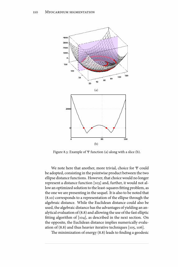
110 Myocardium segmentation
(a)
0 85 150
0
2000
(b)
Figure 8.3: Example of Ψ function (a) along with a slice (b).
We note here that another, more trivial, choice for Ψ couldbe adopted, consisting in the pointwise product between the twoellipse distance functions. However, that choicewould no longerrepresent a distance function [103] and, further, it would not al-low an optimized solution to the least-squares tting problem, asthe one we are presenting in the sequel. It is also to be noted that(8.10) corresponds to a representation of the ellipse through thealgebraic distance. While the Euclidean distance could also beused, the algebraic distance has the advantages of yielding an an-alytical evaluation of (8.8) and allowing the use of the fast elliptictting algorithm of [104], as described in the next section. Onthe opposite, the Euclidean distance implies numerically evalu-ation of (8.8) and thus heavier iterative techniques [105, 106].
eminimization of energy (8.8) leads to nding a geodesic

8.1. Proposed segmentation framework 111
zero level-set (in our case two contours) in a Riemannian spacederived from the shape prior content. As compared to the ini-tial work of [107] and derived approaches [90], the arc lengthfunction of (8.8) is no longer weighted by an image based infor-mation but only by our shape prior term. From the observationthat the minimum of this expression is reached when the zerolevel of ϕ perfectly ts the zero level of the parametric implicitfunction Ψ, one can anticipate that the minimization of this en-ergy criterion will make the level-set evolve toward an annularshape. e numerical minimization of (8.8) is addressed usinga two phase scheme [84, 90]. Specically, keeping λ xed, theminimization of Eshape with respect to ϕ leads to the followingequation:
∂ϕ
∂τ= δ(ϕ(x))g(x, λ) (8.11)
where
g(x, λ) = 2Ψ∇Ψ ⋅ ∇ϕ∣∣∇ϕ∣∣ +Ψ2div( ∇ϕ∣∣∇ϕ∣∣ ) (8.12)
where the dependence of ϕ and Ψ on x has been omitted forcompactness of notation. en, keeping ϕ xed, λ is updatedaccording to the following least-squares tting problem:
λ = argminλ′∮ΓΨ2(s, λ′)ds = argmin
λ′∑x i∈Γ
Ψ2(xi , λ′) (8.13)
By noting that ∣∣∇ϕ∣∣ = 1 because of the signed distance prop-erty [80], then (8.13) corresponds to the exact minimization of(8.8) w.r.t. λ. e rightmost of (8.13) is justied by the fact thatthe image space is in practice discrete. To the best of author’sknowledge, nomethod for the tting of annular shapes has beenproposed yet. We derive such a solution in the following.
Least-squares tting of annular shapes
Considering (8.9), the sum in (8.13) can be rewritten as:
J(x, λ) = ∑x∈ΓA
E 2(x, λout) + ∑x∈ΓB
E 2(x, λin) (8.14)
where the partition Γ = ΓA , ΓB has been introduced
ΓA(λin , λout) = x ∈ Γ∣E(x, λout) ≥ −E(x, λin)ΓB(λin , λout) = x ∈ Γ∣E(x, λout) < −E(x, λin) (8.15)

112 Myocardium segmentation
Input data: λ(0)
in , λ(0)
out , k = 1, tol = 1e-2
Initialization:
E(0) = J[λ(0)in , λ(0)
out];Γ(0)A = ΓA[λ(0)in , λ
(0)
out]; Γ(0)B = ΓB[λ(0)in , λ(0)
out];while e > tol do:
λ(k)
in = tLS[Γ(k−1)B ]; λ(k)
out = tLS[Γ(k−1)A ];Γ(k)A = ΓA[λ(k)in , λ
(k)
out ]; Γ(k)B = ΓB[λ(k)in , λ(k)
out ];E(k) = J[λ(k)in , λ
(k)
out ];e = ∣∣E(k) − E(k−1)∣∣/∣∣E(k−1)∣∣; k = k + 1;
end while
Table 8.1: Least Squares Fitting Algorithm
From this formulation, we observe that (8.14) can be min-imized by tting two separate ellipses on ΓA and ΓB, for whichfast direct solvers exist. Consequently we propose to minimizeJ by alternatively tting the two ellipses and updating ΓA andΓB according to (8.15). e resulting algorithm is summarizedin Table 8.1. By doing so, the energy J is ensured to decrease ateach step. In Table 8.1 we call tLS the function performing thedirect least-squares ellipse tting described in [104].
In Figure 8.4, two examples are reported. In both cases, the
two initial ellipses dened by λ(0)
in and λ(0)
out are coincident. Weadopt at rst three dierent initializations from the same dataset(blue contours in Figure 8.4(a)). In each case, the algorithm con-verges to the same results aer only 3 iterations, as shown inFigure 8.4(b). is shows the robustness of our method with re-spect to the initialization. We then tested our tting algorithmon a more challenging case, where some of the points that de-scribe both the inner and outer contours are superimposed (Fig-ure 8.4(c)). Figure 8.4(d) shows the good behavior of our al-gorithm in such situation. In this case, convergence has beenreached aer only 4 iterations.
e computational complexity of Table 8.1 is dominated by

8.1. Proposed segmentation framework 113
(a) (b)
(c) (d)
Figure 8.4: Illustration of the use of annular least square tting. Inboth cases, the two initial ellipses are coincident. First row:
illustration on a simple case. a) Initialization: the three ellipsescorresponds to three dierent initializations. b) Results obtained atconvergence: the nal annular contours are identical. Second row:illustration on a more challenging case. c) Initialization. d) Results
obtained at convergence aer only 4 iterations.
the few single ellipse least-squares tting operations involved,indicated by the function tLS. As shown in [104], such a prob-lem is equivalent to an eigenvalue problem for a 6×6 matrix,which can be eciently solved with O(n3) oating point oper-ations [108]. As an example, the solution of Table 8.4 is obtainedin 13 ms in a MATLAB (R2010b,e Math Works) implementa-tion of the algorithm, executed on a 2.27GHz Intel Core i5 laptopequipped with 4 GB of RAM and running Windows 7 64-bit.
As detailed in the sequel, the segmentation method consistsin a two stage procedure, i.e.alternating the t of the annularshape to the level-set described in Table 8.1 and the constrained

114 Myocardium segmentation
evolution of the level-set through (8.6). It is then to be noted thatthe tting stage can be made very fast by initializing the algo-rithm inTable 8.1 with the tting result computed at the previousiteration. In practice, the experiments showed that this strategyallows performing the tting stage in one single iteration
As a further remark, it should be noted that, although theframeworkhas been specialized for annular shapes, the proposedformalism is general. In particular it can be extended to geomet-ric primitives for which an ecient solution to the least squarestting problem can be individuated, to be used in place of FitLSin Table 8.1. In this context, an extension of the algorithm to ar-bitrary views of the heart based on hyperquadrics is currentlyunder our investigation [109].
We conclude this section by pointing out that the penaltyterm in (8.8) is not new in literature: Chen et al. introducedan analogous one in [90], in order to embed a shape constraintin the geodesic active contour ow [107]. Nevertheless, the dif-ference between the presented framework and the one in [90]is substantial: in [90] Ψ represents the distance, computed nu-merically, of a point to an arbitrary shape, and consequently asimilarity transformation between the segmenting contour andthe prior shape has to be searched in a steepest descent scheme.In our work, we develop an analytic representation for Ψ, ex-pressed by (8.9), allowing thereby to express the parameters up-date step as a direct least squares tting. As a consequence, thisstage of the algorithm avoids slow steepest descent iterative pro-cedures. ese aspects will be further stressed in the results sec-tion, where a comparison of the proposed algorithm with theone by Chen is presented, both in terms of segmentation accu-racy and execution time.
8.1.3 Collision preventing term
Up to this point the two contours are let to move independentlyone from the other. For this reason there’s the risk for them tocollide by merging into a single contour. It could happen for in-stance in the case the structures of interest are close to each other.is fact would preclude a meaningful segmentation result.
We stress that this situation was never encountered as longas ultrasound images were considered. is was due to the factthat image size was high enough to preserve a sucient distancebetween endo and epicardium. As a consequence, the term weare describing in this section was not considered when dealing
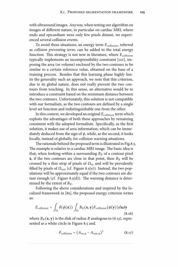
8.1. Proposed segmentation framework 115
with ultrasound images. Anyway, when testing our algorithmonimages of dierent nature, in particular on cardiac MRI, whereendo and epicardium were only few pixels distant, we experi-enced several collision events.
To avoid these situations, an energy term Ecollision , referredas collision preventing term, can be added to the total energyfunction. is strategy is not new in literature, where Ecollision
typically implements an incompressibility constraint [110], im-posing the area (or volume) enclosed by the two contours to besimilar to a certain reference value, obtained on the base of atraining process. Besides that this learning phase highly lim-its the generality such an approach, we note that this criterion,due to its global nature, does not really prevent the two con-tours from touching. In this sense, an alternative would be tointroduce a constraint based on the minimum distance betweenthe two contours. Unfortunately, this solution is not compatiblewith our formalism, as the two contours are dened by a singlelevel set function and indistinguishable one from the other.
In this context, we developed anoriginal Ecollision termwhichexploits the advantages of both these approaches by remainingconsistent with the adopted formalism. Specically, as the rstsolution, it makes use of area information, which can be imme-diately deduced from the sign of ϕ, while, as the second, it lookslocally, instead of globally, for collision warning situations.
e rationale behind the proposed term is illustrated in Fig.8.5.e example is relative to a cardiac MRI image. e basic idea isthat, when looking within a surrounding BR of a contour pixelx, if the two contours are close in that point, then BR will becrossed by a thin strip of pixels of Ωin and will be prevalentlylled by pixels of Ωout (cf. Figure 8.5(e)). Instead, the two pop-ulations will be approximately equal if the two contours are dis-tant enough (cf. Figure 8.5(d)). e warning distance is deter-mined by the extent of BR .
Following the above considerations and inspired by the lo-calized framework in [85], the proposed energy criterion writesas:
Ecollision = ∫Ωδ(ϕ(x))∫
ΩBR(x, y)Fcollision(ϕ(y))dxdy
(8.16)where BR(x, y) is the disk of radius R analogous to (6.13), repre-sented as a white circle in Figure 8.5 and.
Fcollision = (Ain,x − Aout,x)2 (8.17)

116 Myocardium segmentation
(a) (b) (c)
(d) (e)
Figure 8.5: In (a) the two contours soon before the collision. Tworegions, corresponding to a safe distant-contours situation and awarning close-contours situation are represented as white disks. In(b) the active contour aer the collision. In (c) the result obtainedthanks to the collision preventing term. In (d) and (e) a zoom ofthe two regions corresponding to distant and close contoursrespectively. e image is taken from a cardiac MRI exam.
where Ain,x and Aout,x represent the areas of the two sets Ωin,x
and Ωout,x in Figure 8.5, and can be expressed as:
Ain,x = ∫ΩBR(x, y)H(−ϕ(y))dy,
Aout,x = ∫ΩBR(x, y)H(ϕ(y))dy. (8.18)
e eect of (8.16) to keep the two areas Ain,x and Aout,x similar,so preventing the close contours situations of Figure 8.5(e). Us-ing the general framework in [85] the minimization of Ecollision
with respect to ϕ leads to:
∂ϕ
∂τ= h(x)δ(ϕ(x)) (8.19)
where

8.2. Implementation issues 117
h(x) = 2∫Ωδ(ϕ(y))BR(x, y)(Ain,x − Aout,x). (8.20)
An example of the eect of this term is illustrated in Fig-ure 8.5(c). Note that no collision happens thanks to the proposedterm and ameaningful result is obtained. e value of ρ has beenxed equal to 5 pixels in that case.
We conclude this section with a remark. e term in (8.17)does not distinguish between close contours and peaky corners,indeed in this second circumstance as well the number of inside-pixelsmay be substantially smaller than the outside-ones. oughthis factmay represent a shortcoming in general, since it hindersthe detection of high curvature details, otherwise this is not thecase for the application at hand, in which the interesting patterscan be represented by ellipses and therefore present an intrinsicsmoothness.
8.2 Implementation issues
Level-set evolution equation is implemented using a standard -nite dierence scheme [80], where the implicit function ϕ is rep-resented by a signed distance function. In order to improve e-ciency, values of ϕ are only computed in a narrow band aroundthe zero level set. Consequently, ϕ is re initialized every few iter-ations using a fast marching scheme [80]. e nal, shape-priorlevel set equation, writes as:
∂ϕ
∂τ(x) = δ(ϕ(x)) [ f (x) + α ⋅ g(x, λ)] (8.21)
where f and g are dened as in (8.6) and (8.12) respectively. echoice of the weight term α is dependent on the specic appli-cation. For instance, when the quality of the image is poor, itis recommended to use higher value of α in order to put moreimportance on the shape prior term. When presenting resultsin the experiments section, we will adopt the α value which pro-duces the best segmentation result. In particular a value α =1.2was found to produce the best result on available images.
Concerning the initialization, let us note the localized frame-work of [85] requires that this is made not too far from the de-sired solution. Indeed while such a local data attachment termallowsmaking the algorithmmore robust to the variation of im-age properties, it makes it more sensitive to initialization. In theexperiments described in the next sections, the following sim-ple procedure is thus considered. e user is asked to position
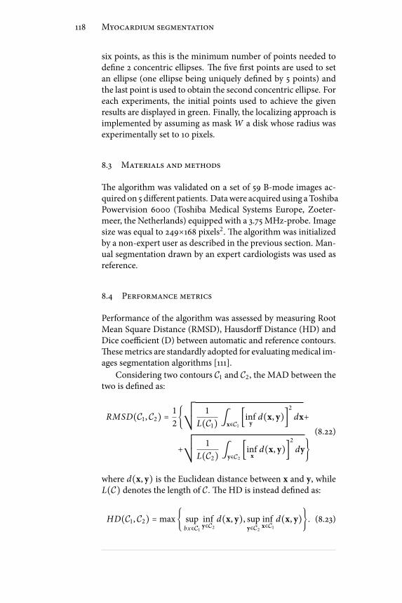
118 Myocardium segmentation
six points, as this is the minimum number of points needed todene 2 concentric ellipses. e ve rst points are used to setan ellipse (one ellipse being uniquely dened by 5 points) andthe last point is used to obtain the second concentric ellipse. Foreach experiments, the initial points used to achieve the givenresults are displayed in green. Finally, the localizing approach isimplemented by assuming as mask W a disk whose radius wasexperimentally set to 10 pixels.
8.3 Materials and methods
e algorithm was validated on a set of 59 B-mode images ac-quired on 5 dierent patients. Datawere acquired using aToshibaPowervision 6000 (Toshiba Medical Systems Europe, Zoeter-meer, the Netherlands) equipped with a 3.75 MHz-probe. Imagesize was equal to 249×168 pixels2. e algorithm was initializedby a non-expert user as described in the previous section. Man-ual segmentation drawn by an expert cardiologists was used asreference.
8.4 Performance metrics
Performance of the algorithm was assessed by measuring RootMean Square Distance (RMSD), Hausdor Distance (HD) andDice coecient (D) between automatic and reference contours.esemetrics are standardly adopted for evaluatingmedical im-ages segmentation algorithms [111].
Considering two contours C1 and C2, the MAD between thetwo is dened as:
RMSD(C1 , C2) = 1
2¿ÁÁÀ 1
L(C1) ∫x∈C1 [infy d(x, y)]2 dx++
¿ÁÁÀ 1
L(C2) ∫y∈C2 [infx d(x, y)]2 dy(8.22)
where d(x, y) is the Euclidean distance between x and y, whileL(C) denotes the length of C. e HD is instead dened as:
HD(C1 , C2) =max supbx∈C1
infy∈C2
d(x, y), supy∈C2
infx∈C1
d(x, y). (8.23)

8.5. Results 119
Dice HD RMSD
with shape prior 0.89±0.02 5.57±1.18 2.22±0.46
without shape prior 0.87±0.03 7.78±2.12 2.55±0.49
Table 8.2: Performance metrics value (mean ± standarddeviation) for the proposed algorithm on 59 echocardiographic
images, respectively with (α=1.2) and without (α=0) shapeinformation.
Finally, dening Ω1 and Ω2 as the sets of pixels enclosed bythe closed contours C1 and C2, the Dice coecient writes as:
D(Ω1 , Ω2) = 2 #(ΩS⋂ΩR)#(Ω1) + #(Ω2) (8.24)
where #(⋅) extracts the set cardinality.e RMSD measures the average distance between the two
contours, and is thus suited for evaluating the global performanceof the algorithm. On the opposite, the Haussdorf metric repre-sents themaximumdistance between the contours, and is there-fore a local index of performance [112]. More specically, theHD keeps trace of the localized discrepancies which are largelyhidden in the average operation involved in the RMSD compu-tation. While RMSD andHDdepend on the image size, theDicecoecient returns instead an intrinsic index of performance, sinceit measures the superposition in percentage between the two en-closed areas. ese three metrics are adopted to provide an ex-haustive evaluation of the behavior of the proposed algorithm.
8.5 Results
8.5.1 Evaluation of shape prior contribution
In order to evaluate the eect of the shape prior informationwe ran our algorithm with and without using the shape priorterm. When the shape information was taken into account avalue α=1.2 was used. e complete set of results is reported inTable 8.2. is table clearly shows that the introduction of theshape prior yields an improvement of the segmentation, yield-ing a slightly higher Dice and smaller HD and RMSD.
Figure 8.6 provides segmentation examples allowing a nerinterpretation of these results. It may be observed that the shapeprior allows to avoid the local irregularities, linked to the attrac-tion of the active contours to small scale noisy structures. is

120 Myocardium segmentation
(a) (b)
Figure 8.6: Manual reference and segmentation result as a thin andcontinuous line respectively. Note how the shape constraintprevents the contour from adhering to irregularities in the
endocardium (white arrow in (a)), principally ascribable to thepresence of the papillary muscles. In general much regular resultsare obtained with the shape prior approach, with an augmentedcorrespondence with the cardiologist reference. Error metrics forthose images are: (a) HD=14.3, RMSD=5.35, D=0.83; (b) HD=5.83,
RMSD=2.52, D=0.89.
explains in particular the large decrease of HD associated withthe shape information.
8.5.2 Comparison with Chen algorithm
We compare in this section the performance of our algorithmwith the approach described in [90]. e basic equations forChen algorithm are reported in Appendix D. e use of Chen’sapproach implies the learning of the shape prior through a train-ing phase performed on a set of manually segmented contours.In this experiment, the prior contourwas obtained for eachmod-ality from a training image set, built by randomly selecting ref-erence contours. Specically, 10 images out of 59 were used. eprior contour was obtained by averaging the reference contoursdrawn by the physician. Due to potential misalignment amongthe references, a registration stepmust precede the averaging op-eration, as detailed in [90]. e so obtained prior contour is il-lustrated in Figure 8.7(b). From this gure it can also be clearlyseen that ellipses represent a reliable approximation of myocar-

8.5. Results 121
50 60 70 80 90 10040
45
50
55
60
65
70
75
80
85
90
MRI reference contour
(a)
0 20 40 60 80 100 120 1400
50
100
150
US reference contour
(b)
Figure 8.7: Prior contour computation for (a) MRI and (b)ultrasound images. e cluster of reference curves is represented asthin contours and the corresponding average shape as a bold red
contour.
Dice HD RMSD
proposed algorithm 0.89±0.02 5.57±1.18 2.22±0.46
chen’s algorithm 0.86±0.03 8.05±1.55 2.50±0.72
Table 8.3: Performance metrics value (mean ± standarddeviation) for the proposed algorithm and Chen’s one for US
images. e training images are eliminated from the data set beforeevaluation. e total number of testing images is the equal to 49.
dial contours.e complete set of results is reported in Table 8.3. ese
results clearly show that the proposed algorithm outperformsChen’s approach for the present application. Let us note thatthe dierence in performance is particularly pronounced for theHausdor distance. is behavior is linked to the fact that inChen’s approach, the only non-rigid degree of freedom appliedto the shape prior in the course of the segmentation is a uniformscaling. On the opposite, our approach performs a complete tof the prior at each iteration, thus yielding a better adjustmentto the myocardial shape variations.
Another important issue concerns the computational speed.e average cpu time needed for segmenting one image was 13.5seconds for our method and 36.7 seconds for Chen’s method.is speed-up is a consequence of the availability of a paramet-ric representation for the prior, combined with the existence ofa fast tting procedure for such a geometry. In particular, the

122 Myocardium segmentation
most costly step in Chen’s algorithm is the initial alignment ofthe prior shape onto the initial contour (cf. AppendixD). For theconsidered images, this step can take up to several thousands ofiterations. On the opposite, in our approach the initial registra-tion corresponds to t the initial contour with an annular shape,which is typically done in few iterations.
8.6 Beyond ultrasound
Due to its extremeexibility, the shape prior segmentation frame-work described in this chapter, can be suitably applied to everykind of image containing annular-like patterns. Indeed similarpatterns are recurrent in images from several elds: medicine,biology and astronomy are some examples. In this section wepresent some results obtained on various natural images and oncardiac MRI.
As all those images are less challenging thanUS, the sophisti-cated statistical framework described in §8.1.1 is no longer nec-essary and the standard Chan-Vese framework, in its localizedversion, has been proved to be largely sucient.
8.6.1 Segmentation of natural images
Figure 8.8 illustrates the application of the proposed method forthe segmentation of the pupil and iris in human eye, of the zonapellucida in human embryo, and the rings of Saturn. We usedfor these experiments the same α value equal to 0.8. We ob-serve that in all those situations gray scale information alone isnot sucient for obtaining correct results. In the eye image (Fig-ure 8.8(a)), the eyelash hinders a correct iris detection,moreoverthe variations in the iris color make pupil segmentation impre-cise. A similar eect can be observed in the embryo image (Fig-ure 8.8(b)) where the segmentation is inaccurate due to low con-trast proles and to proximity of the cell to the internal bound-ary of the zona pellucida. In the Saturn image, the ring portionhidden by the planet body cannot be followed without a shapeprior approach (Fig.8.8(c)).
e results obtained using the shape prior term are given inthe second row. In the 3 cases, they are in good agreement withthe expected shapes. ey illustrate the usefulness of the pro-posed annular shape prior for such images. Regarding the com-putational cost, Table 8.4 provides the cpu times correspondingto the segmentations performed with our approach and shown

8.6. Beyond ultrasound 123
(a) (b) (c)
(d) (e) (f)
Figure 8.8: Segmentation results obtained on natural scene images.e green points correspond to the initialization. Images (a) to (c)show the result obtained when the proposed approach is appliedwithout the shape constraint. Images (d) to (f) show the result
obtained when the shape prior is applied.
Eye image Embryo image Saturn image
(Fig.8.8(d)) (Fig.8.8(d)) (Fig.8.8(f))
Overall 8.31 17.93 13.86
shape fitting 0.12 0.33 0.36
Table 8.4: Cpu time (s) corresponding to the segmentation with theproposed approach on natural images.
in Figure 8.8(d) to Figure 8.8(f). Note that the 3 images sharethe same size 200x200 pixels. In order to give an insight on theimpact of the shape prior termon the overall computational bur-den, Table 8.4 also gives the cpu time corresponding to the t-ting step of the algorithm in §8.1.2. ese results conrm that theimprovements in segmentation accuracy ascribable to the shapeprior term come at a substantially negligible price in terms ofcomputational complexity.

124 Myocardium segmentation
Dice HD RMSD
with shape prior 0.82±0.05 3.63±0.73 1.46±0.21
without shape prior 0.80±0.05 4.62±0.82 1.72±0.27
Table 8.5: Performance metrics value (mean ± standarddeviation) for the proposed algorithm on 56 cardiac MRI images,respectively with (α=0.8) and without (α=0) shape information.
8.6.2 Segmentation of cardiac MRI
e algorithm has been evaluated on a set of 52 cardiacMRI im-ages. A value α =0.8 was used to balance the shape prior in-uence. We note that this is smaller than the one adopted forultrasound as MRI has an intrinsically higher image quality. Asmentioned, due to the reduced size of MRI images, endo andepicardium happened to be too close to prevent collision be-tween the two contours. Consequently the collision preventingenergy term presented in §8.1.3 was added to the energy func-tion, weighted by an opportune hyper parameter β. A valueβ=0.4 was experimentally found to avoid collision events on allthe available images. A value R=4 pixels was adopted for the cor-responding collision indicator BR . e same set of experimentsperformed for US were made for MRI and are reported in thissection.
From the evaluation of the shape prior contribution we ob-tained the results reported in Table 8.5. Note that both HD andRMSDhave smaller values forMRI than forUSdue to the smallersize of the former. A visual comparison between the shape priorand the shape free approach is reported in Figure 8.9.
A comparison with Chen algorithm is presented as well. Inthis case the prior shape was built from a training set composedof 10 out of the 56 images. e so obtained reference contour isillustrated in Figure 8.7(a). e obtained results are reported inTable 8.6. An example image is illustrated in Figure 8.10.
8.6.3 Dependence on the initialization
As previously mentioned, the adoption of the localized frame-work of [85] imposes a good initialization in order to guaranteeadequate results. In practice, this implies that the distance be-tween the initial contour and the object to be detected should beon the order of the extent of the maskW(⋅). In this section, wethus propose to study the inuence of initialization by applying a

8.6. Beyond ultrasound 125
(a) (b)
Figure 8.9: Segmentation results on cardiac MRI. Manual referenceand segmentation result as a dashed and continuous line
respectively. Note how the shape constraint prevents the contourfrom adhering to the right ventricle (upper arrow in (a)) and
allows to cope with the low contrast of the endocardium (lowerarrow in (a)). Error metrics for those images are: (a) HD=5,RMSD=1.52, D=0.83; (c) HD=2.23, RMSD=0.99, D=0.89;(b)
HD=2.23, RMSD=0.99, D=0.89.
Dice HD RMDS
proposed algorithm 0.82±0.05 3.63±0.73 1.46±0.21
chen’s algorithm 0.76±0.18 4.89±1.06 1.74±0.45
Table 8.6: Performance metrics value (mean ± standarddeviation) for the proposed algorithm and Chen’s one for MRI
images. e training images are eliminated from the data set beforeevaluation. e total number of testing images is the equal to 46.
random variation to the location of the 6 points used in our ini-tialization procedure. Although the study is presented here forMRI images only, the considerations that follow are absolutelygeneral.
is experiment is illustrated in Figure 8.11 and is done asfollows. We delineate from a specic MRI image six regions inwhich initial points are randomly positioned (red disk in Fig-ure 8.11(a)). Each region corresponds to a disk with a radius of3 pixels. is dimension has been chosen to simulate the un-certainty in the positioning of the points by the user. In or-der to show the inuence of such random scheme in the initial-

126 Myocardium segmentation
PROPOSED
REFERENCE
RESULT
30 40 50 60 70 80 90 100 110
30
40
50
60
70
80
90
100
110
(a) (b)
RESULT
PRIOR
30 40 50 60 70 80 90 100 110
30
40
50
60
70
80
90
100
110
(c)
Figure 8.10: Comparison between the proposed (a) and Chen (b)algorithm applied to an MRI image. e prior for Chen algorithmis not appropriate for this particular frame and compensates forthe lack of data information in a way which is not consistent withthe real heart morphology, as shown by the arrows in (b) and (c).Dierently, the adopted parametric formulation easily allows to
second myocardial shape. Error measures are: (a) D=0.87,HD=3.60 and RMSD=1.42; (b) D=0.76, HD=5.88 and RMSD=2.09.
ization, we display in Figure 8.11(a) two particular initial con-tours obtained from the proposed random initializations andFigure 8.11(b) shows the nal contours obtained from 10 dier-ent initializations. In order to evaluate the variability of the re-sulting segmentations, we compute the similarity measures byconsidering all the possible combinations of two nal contours.Weobtainedmean values ofD=0.98,HD=1.1 pixels andRMSD=0.3pixels. ese values illustrate the robustness of the proposedmethod with respect to the initialization phase.
As a conclusion, although the local data attachment term im-plies an initialization close to the desired contour, within thislimit, this initialization thus needs not to be very accurate.
8.7 Conclusion
in this chapter a novel framework based on level-sets has beenintroduced and described. e algorithm contains several ele-ments of novelty over the related literature, specically:
• a parametric implicit function dening the distance fromtwo ellipses is introduced;
• an ecient solution to the least- squares tting problemof annular shapes is developed;
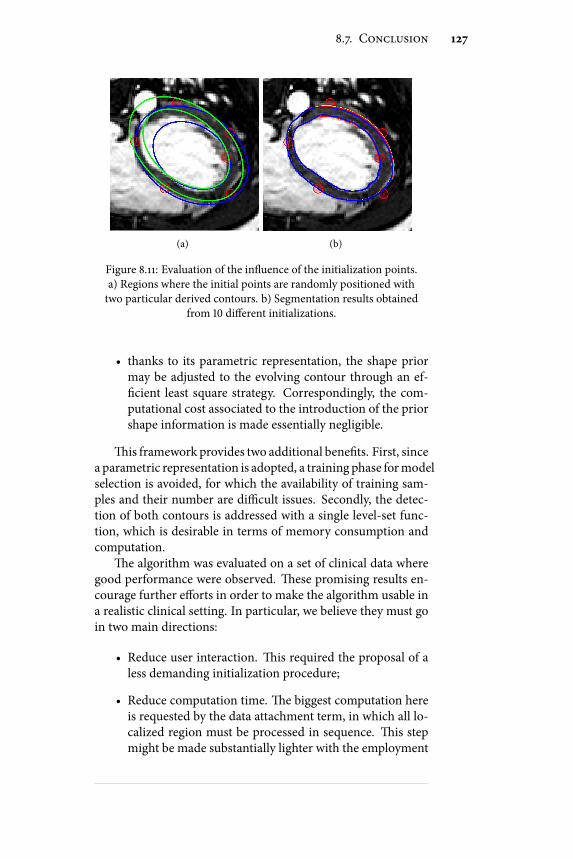
8.7. Conclusion 127
(a) (b)
Figure 8.11: Evaluation of the inuence of the initialization points.a) Regions where the initial points are randomly positioned withtwo particular derived contours. b) Segmentation results obtained
from 10 dierent initializations.
• thanks to its parametric representation, the shape priormay be adjusted to the evolving contour through an ef-cient least square strategy. Correspondingly, the com-putational cost associated to the introduction of the priorshape information is made essentially negligible.
is framework provides two additional benets. First, sincea parametric representation is adopted, a training phase formodelselection is avoided, for which the availability of training sam-ples and their number are dicult issues. Secondly, the detec-tion of both contours is addressed with a single level-set func-tion, which is desirable in terms of memory consumption andcomputation.
e algorithm was evaluated on a set of clinical data wheregood performance were observed. ese promising results en-courage further eorts in order to make the algorithm usable ina realistic clinical setting. In particular, we believe they must goin two main directions:
• Reduce user interaction. is required the proposal of aless demanding initialization procedure;
• Reduce computation time. e biggest computation hereis requested by the data attachment term, in which all lo-calized region must be processed in sequence. is stepmight be made substantially lighter with the employment

128 Myocardium segmentation
of GPU programming techniques, which would allow toexploit the parallelism oered by modern GPUs architec-tures.

Chapter 9Conclusion
This manuscript described the research activity carriedout by the author between January 2008 and December2010 in the context of his PhD at the Advanced Research
Center on Electronic Systems and Information Technology ofthe University of Bologna, Italy. Part of the work was made dur-ing a one year internship within the ultrasound team of the theCentre de Recherche et d’Applications en Traitement de l’Imageet du Signal (CREATIS) in Lyon, France.
Two major topics inherent with medical ultrasound imageswere addressed during the PhD research. erst project had itsprincipal goal in the development of an eective pre-processingtool for reducing system dependencies in the performance ofultrasound based tissue characterization algorithms. is wasmade possible thanks to the proposal of an original deconvolu-tion framework allowing to restore statistically consistent max-imum a posteriori estimates of the tissue reectivity. A perfor-mance evaluation was documented in the thesis, obtained fromphantom data mimicking biological tissues with dierent par-ticle concentrations. e results showed a relevant decrease inthemisclassication error when processed data were consideredinstead of the raw signal, along with the superiority of the pro-posed paradigmover standard deconvolution tools. Futureworkmust include the validation of the proposed scheme on clinicaldata. In this sense the main interest relies in the detection ofpotentially cancerous areas on trans rectal ultrasound images ofthe prostate for guiding biopsy procedures.
e second activity stemmed instead from the purpose toprovide the cardiology communitywith soware tools for easing
129

130 Conclusion
the reading and analysis of echocardiographic sequences. In thiscontext a semi-automatic segmentation tool for joint detectionof endo- and epicardial contours from short axis acquisition wasdesigned. e algorithm was derived on the base of the level-set formalism and eectively incorporated information on sig-nal statistics andmyocardium expected geometry for constrain-ing the results to anatomically meaningful shapes. e obtainedresults have shown that the proposed algorithm can reduce thehigh inter- and intra-operator variability and is feasible and ac-curate even for realistic clinical data. A natural continuation ofthis activity includes the generalization of the proposed frame-work to the case of arbitrary probe orientations, in this sensesome preliminary results have been recently obtained [P1][P6],and the use of the detected contours for the calculation of pa-rameters commonly adopted in the clinical routine for the diag-nosis of heart disease as ejection fraction and wall thickening.
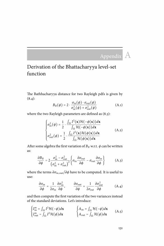
Appendix ADerivation of the Bhattacharyya level-setfunction
e Bathhacharyya distance for two Rayleigh pdfs is given by(8.4):
BR(ϕ) = 2 ⋅ σin(ϕ) ⋅ σout(ϕ)σ 2in(ϕ) + σ 2
out(ϕ) (A.1)
where the two Rayleigh parameters are dened as (8.3):
⎧⎪⎪⎪⎪⎪⎪⎪⎨⎪⎪⎪⎪⎪⎪⎪⎩
σ 2in(ϕ) = 1
2⋅ ∫Ω I2(x)H(−ϕ(x))dx∫ΩH(−ϕ(x))dx
σ 2out(ϕ) = 1
2⋅ ∫Ω I2(x)H(ϕ(x))dx∫ΩH(ϕ(x))dx
(A.2)
Aer some algebra the rst variation of BR w.r.t. ϕ can bewrittenas:
∂BR
∂ϕ= 2 σ 2
in − σ2out(σ 2
in + σ2out)2 σin
∂σout∂ϕ− σout
∂σin∂ϕ (A.3)
where the terms ∂σin,out/∂ϕ have to be computed. It is useful touse:
∂σin∂ϕ= 1
2σin
∂σ 2in
∂ϕ,
∂σout∂ϕ= 1
2σout
∂σ 2out
∂ϕ(A.4)
and then compute the rst variation of the two variances insteadof the standard deviations. Let’s introduce:⎧⎪⎪⎨⎪⎪⎩
Imin = ∫Ω I2H(−ϕ)dxImout = ∫Ω I2H(ϕ)dx
⎧⎪⎪⎨⎪⎪⎩Ain = ∫ΩH(−ϕ)dxAout = ∫ΩH(ϕ)dx (A.5)
131

132 Derivation of the Bhattacharyya level-set function
where the dependency of I and ϕ on x has been omitted. eseallow to write:
∂σ 2in
∂ϕ= 1
A2in
∂Imin∂ϕ
Ain −∂Ain
∂ϕImin (A.6)
By using the theory of variations, it is:
∂Imin∂ϕ= −I2δ(ϕ), ∂Ain
∂ϕ= −δ(ϕ) (A.7)
and, aer some calculation:
∂σin∂ϕ= σinAin − I2
2σ 2in
+ 1δ(ϕ). (A.8)
Analogously one can derive the same expression for σout:
∂σout∂ϕ= σoutAout I2
2σ 2out
− 1δ(ϕ). (A.9)
By substituting (A.8) and (A.9) into (A.3), the nal expressioncan be obtained:
∂BR
∂ϕ= BR
2[σ 2
out − σ2in
σ 2in + σ
2out
][ 1
Aout( I2(x)2σ 2
out
− 1)++
1
Ain( I2(x)2σ 2
in
− 1)]δ(ϕ).(A.10)

Appendix B
Computation of spatially-variant blurringoperators
B.1 Spatially invariant PSF
Consider the image formation process:
Y = P ∗ X (B.1)
where X ∈MN×M is the real data and Y ∈MN×M is the obser-vation, obtained with the kernel P ∈Mn×m .
It’s common to represent the observation process in matrixvector notation:
y = Hx
where x and y are the column vectors obtained via lexicographi-cal ordering of X andY . Herewewant to showhowH ∈MNM×NM
looks like for case N = 9, M = 5, n = 3, m = 3.Whenperforming the convolution operation, boundary con-
ditions for X have to be specied. Specically, this is done bypadding of n − 1 elements in the axial direction, and m − 1 inthe lateral one. For computational reasons we will consider here
133

134 Computation of spatially-variant blurring operators
circular padding. e padded matrix becomes:
Xp =
⎡⎢⎢⎢⎢⎢⎢⎢⎢⎢⎢⎢⎢⎢⎢⎢⎢⎢⎢⎢⎢⎢⎢⎢⎢⎣
x8,4 x8,5 x8,1 x8,2 x8,3 x8,4 x8,5
x9,4 x9,5 x9,1 x9,2 x9,3 x9,4 x9,5
x1,4 x1,5 x1,1 x1,2 x1,3 x1,4 x1,5
x2,4 x2,5 x2,1 x2,2 x2,3 x2,4 x2,5
x3,4 x3,5 x3,1 x3,2 x3,3 x3,4 x3,5
x4,4 x4,5 x4,1 x4,2 x4,3 x4,4 x4,5
x5,4 x5,5 x5,1 x5,2 x5,3 x5,4 x5,5
x6,4 x6,5 x6,1 x6,2 x6,3 x6,4 x6,5
x7,4 x7,5 x7,1 x7,2 x7,3 x7,4 x7,5
x8,4 x8,5 x8,1 x8,2 x8,3 x8,4 x8,5
x9,4 x9,5 x9,1 x9,2 x9,3 x9,4 x9,5
⎤⎥⎥⎥⎥⎥⎥⎥⎥⎥⎥⎥⎥⎥⎥⎥⎥⎥⎥⎥⎥⎥⎥⎥⎥⎦where padded elements are includedwithin boxes for clarity pur-poses.
Let’s call pij the generic element of P and introduce the Cir-culant matrix Pk ∈MN×N
Pk =
⎡⎢⎢⎢⎢⎢⎢⎢⎢⎢⎢⎢⎢⎢⎢⎢⎢⎢⎢⎣
p1k 0 0 0 0 0 0 p2k p3kp2k p1k 0 0 0 0 0 0 p3kp3k p2k p1k 0 0 0 0 0 00 p3k p2k p1k 0 0 0 0 00 0 p3k p2k p1k 0 0 0 00 0 0 p3k p2k p1k 0 0 00 0 0 0 p3k p2k p1k 0 00 0 0 0 0 p3k p2k p1k 00 0 0 0 0 0 p3k p2k p1k
⎤⎥⎥⎥⎥⎥⎥⎥⎥⎥⎥⎥⎥⎥⎥⎥⎥⎥⎥⎦
(B.2)
Let’s note that the matrix corresponds to the 1D convolution ofthe k − th column of P with a vector of N entries.
e H matrix then writes as
H =⎡⎢⎢⎢⎢⎢⎢⎢⎢⎢⎣
P1 P3 P2
P2 P1 P3
P3 P2 P1 P3 P2 P1 P3 P2 P1
⎤⎥⎥⎥⎥⎥⎥⎥⎥⎥⎦(B.3)
where is a N × N matrix with all entries equal to 0. MatrixH is so made out of M ×M blocks of N × N circular matrices,and is therefore referred as block circulant with circulant blocks(BCCB). is property is desirable since it makes H diagonaliz-able via 2D Fourier transform, i.e.:
Y = ifft2D(fft2D(P) ⋅ fft2D(X)) (B.4)
If zero padding is chosen instead then Y can be obtained from:
Ypadded = ifft2D(fft2D(P)fft2D(Xpadded)) (B.5)

B.2. Spatially variant PSF 135
aer discarding rows and columns corresponding to the paddedelements.
B.2 Spatially variant PSF
Suppose now that X is blurred with dierent kernels at dierentdepths. We represent these regions with dierent capital lettersA, B and C and represent an entry of X belonging to one of theseregions with a convenient apex.
X =
⎡⎢⎢⎢⎢⎢⎢⎢⎢⎢⎢⎢⎢⎢⎢⎢⎢⎢⎢⎢⎢⎢⎢⎢⎢⎣
xA11 xA
12 xA13 xA
14 xA15
xA21 xA
22 xA23 xA
24 xA25
xA31 xA
32 xA33 xA
34 xA35
xB11 xB12 xB13 xB14 xB15
xB21 xB22 xB23 xB24 xB25
xB31 xB32 xB33 xB34 xB35
xC11 xC12 xC13 xC14 xC15
xC21 xC22 xC23 xC24 xC25
xC31 xC32 xC33 xC34 xC35
⎤⎥⎥⎥⎥⎥⎥⎥⎥⎥⎥⎥⎥⎥⎥⎥⎥⎥⎥⎥⎥⎥⎥⎥⎥⎦
=⎡⎢⎢⎢⎢⎢⎢⎣
XA
XB
XC
⎤⎥⎥⎥⎥⎥⎥⎦(B.6)
We introduce the three blurring operators corresponding tothe three regions as:
PL =⎡⎢⎢⎢⎢⎢⎢⎣
pL11 pL12 pL13
pL21 pL22 pL23
pL31 pL32 pL33
⎤⎥⎥⎥⎥⎥⎥⎦(B.7)
with L ∈ A, B,C. If we assume a piecewise constant inter-polation between the dierent kernels, then the global blurring

136 Computation of spatially-variant blurring operators
matrix equivalent to (B.2) becomes:
Pk =
⎡⎢⎢⎢⎢⎢⎢⎢⎢⎢⎢⎢⎢⎢⎢⎢⎢⎢⎢⎢⎢⎢⎢⎢⎢⎢⎢⎢⎢⎢⎢⎢⎢⎢⎣
pA1k 0 0 0 0 0 0 0 0
pA2k pA1k 0 0 0 0 0 0 0
pA3k pA2k pA1k 0 0 0 0 0 0
0 pB3k pB2k pB1k 0 0 0 0 0
0 0 pB3k pB2k pB1k 0 0 0 0
0 0 0 pB3k pB2k pB1k 0 0 0
0 0 0 0 pC3k pC2k pC1k 0 0
0 0 0 0 0 pC3k pC2k pC1k 0
0 0 0 0 0 0 pC3k pC2k pC1k
⎤⎥⎥⎥⎥⎥⎥⎥⎥⎥⎥⎥⎥⎥⎥⎥⎥⎥⎥⎥⎥⎥⎥⎥⎥⎥⎥⎥⎥⎥⎥⎥⎥⎥⎦
(B.8)
where the sub-matrices corresponding to the single, space in-variant kernels have been enclosed with black contours. e as-sociated H is then build as:
H =⎡⎢⎢⎢⎢⎢⎢⎢⎢⎢⎣
P1 P2 P1 P3 P2 P1 P3 P2 P1 P3 P2 P1
⎤⎥⎥⎥⎥⎥⎥⎥⎥⎥⎦(B.9)
Note that linear convolution is considered instead of circularone. As noticed, this does not prevent fast computation since itjust needs a padding operation on the input. By introducing thematrices corresponding to the single kernels:
PLk =
⎡⎢⎢⎢⎢⎢⎢⎢⎢⎢⎢⎢⎢⎢⎢⎢⎢⎢⎢⎢⎣
pL1k 0 0 0 0 0 0 0 0pL2k pL1k 0 0 0 0 0 0 0pL3k pL2k pL1k 0 0 0 0 0 00 pL3k pL2k pL1k 0 0 0 0 00 0 pL3k pL2k pL1k 0 0 0 00 0 0 pL3k pL2k pL1k 0 0 00 0 0 0 pL3k pL2k pL1k 0 00 0 0 0 0 pL3k pL2k pL1k 00 0 0 0 0 0 pL3k pL2k pL1k
⎤⎥⎥⎥⎥⎥⎥⎥⎥⎥⎥⎥⎥⎥⎥⎥⎥⎥⎥⎥⎦
(B.10)
and the correspondingHL built as in (B.3), then the interpo-lated H can be written as
H = ∑L
DL ⋅HL (B.11)
Where the diagonal matrices DL have their entry ( j, j) equal toone if the j− th pixel in x belongs to the region L, otherwise this
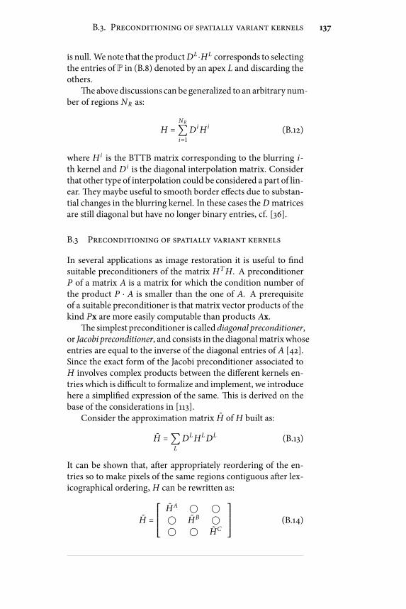
B.3. Preconditioning of spatially variant kernels 137
is null. Wenote that the productDL ⋅HL corresponds to selectingthe entries of P in (B.8) denoted by an apex L and discarding theothers.
e above discussions can be generalized to an arbitrary num-ber of regions NR as:
H = NR∑i=1
D iH i (B.12)
where H i is the BTTB matrix corresponding to the blurring i-th kernel and D i is the diagonal interpolation matrix. Considerthat other type of interpolation could be considered a part of lin-ear. eymaybe useful to smooth border eects due to substan-tial changes in the blurring kernel. In these cases the Dmatricesare still diagonal but have no longer binary entries, cf. [36].
B.3 Preconditioning of spatially variant kernels
In several applications as image restoration it is useful to ndsuitable preconditioners of the matrix HTH. A preconditionerP of a matrix A is a matrix for which the condition number ofthe product P ⋅ A is smaller than the one of A. A prerequisiteof a suitable preconditioner is that matrix vector products of thekind Px are more easily computable than products Ax.
e simplest preconditioner is calleddiagonal preconditioner,or Jacobi preconditioner, and consists in the diagonalmatrixwhoseentries are equal to the inverse of the diagonal entries of A [42].Since the exact form of the Jacobi preconditioner associated toH involves complex products between the dierent kernels en-tries which is dicult to formalize and implement, we introducehere a simplied expression of the same. is is derived on thebase of the considerations in [113].
Consider the approximation matrix H of H built as:
H = ∑L
DLHLDL (B.13)
It can be shown that, aer appropriately reordering of the en-tries so to make pixels of the same regions contiguous aer lex-icographical ordering, H can be rewritten as:
H =⎡⎢⎢⎢⎢⎢⎣
HA HB HC
⎤⎥⎥⎥⎥⎥⎦(B.14)
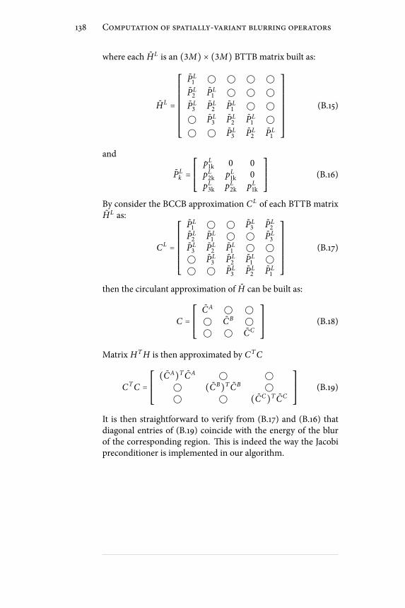
138 Computation of spatially-variant blurring operators
where each HL is an (3M) × (3M) BTTB matrix built as:
HL =⎡⎢⎢⎢⎢⎢⎢⎢⎢⎢⎢⎢⎣
PL1
PL2 PL
1 PL3 PL
2 PL1
PL3 PL
2 PL1
PL3 PL
2 PL1
⎤⎥⎥⎥⎥⎥⎥⎥⎥⎥⎥⎥⎦(B.15)
and
PLk =⎡⎢⎢⎢⎢⎢⎣
pL1k 0 0pL2k pL1k 0pL3k pL2k pL1k
⎤⎥⎥⎥⎥⎥⎦(B.16)
By consider the BCCB approximation CL of each BTTB matrixHL as:
CL =⎡⎢⎢⎢⎢⎢⎢⎢⎢⎢⎣
PL1 PL
3 PL2
PL2 PL
1 PL3
PL3 PL
2 PL1
PL3 PL
2 PL1
PL3 PL
2 PL1
⎤⎥⎥⎥⎥⎥⎥⎥⎥⎥⎦(B.17)
then the circulant approximation of H can be built as:
C =⎡⎢⎢⎢⎢⎢⎣
CA CB CC
⎤⎥⎥⎥⎥⎥⎦(B.18)
Matrix HTH is then approximated by CTC
CTC =⎡⎢⎢⎢⎢⎢⎣(CA)T CA (CB)T CB (CC)T CC
⎤⎥⎥⎥⎥⎥⎦(B.19)
It is then straightforward to verify from (B.17) and (B.16) thatdiagonal entries of (B.19) coincide with the energy of the blurof the corresponding region. is is indeed the way the Jacobipreconditioner is implemented in our algorithm.

Appendix CComplex Generalized GaussianDistribution
Consider the complex random variable z = xr + jx i , where bothxr and x i obey a GGD with zero mean, variance σ 2 and shapeparameter ξ. Assuming mutual independence of xr and x i , thenp(z) = p(xr)p(x i) [16], where p(xr) and p(x i) are dened asin (5.1). Hence it is:
p(z) = a2 exp( − ∣xrb∣ξ − ∣x i
b∣ξ) (C.1)
and correspondingly ln p(z) ∝ (∣xr ∣ξ + ∣x i ∣ξ), which, unlessξ = 2, is dierent from ∣z∣ξ . is fact prevents the restorationproblem to be formalized as an l p-norm optimization task.
Hereto, in order to preserve the desired formalism, we denehere a variation of the GGD for complex variables, which writesas:
p(z) = a2 exp( − ∣ zd∣ξ) (C.2)
where d is determined so to satisfy the normalization condition
∫ ∫ p(z)dx idxr = 1, which leads to
d = b ⋅√2/ξ ⋅ Γ(2/ξ)√Γ(2/ξ) ⋅√π
(C.3)
e requested integral can be easily computed by substitutingz = ρ exp( jθ), so that dxrdx i = ρdρdθ.
Let’s note that in (C.2) the real and imaginary part of z areno longer independent. In particular, the pdf (C.3) is an approx-imation of the one in (C.1), so that the phase0 z is uniformly
139

140 Complex Generalized Gaussian Distribution
−3−2
−10
12
3
−3
−2
−1
0
1
2
3
0.05
0.1
0.15
0.2
0.25
0.3
0.35
0.4
0.45
xr
xi
(a)
−3−2
−10
12
3
−3
−2
−1
0
1
2
3
0.05
0.1
0.15
0.2
0.25
0.3
0.35
0.4
0.45
xr
xi
(b)
Figure C.1: In (a) the pdf in (C.1) is displayed, while in (b) the pdf(C.2). e two pdfs are displayed for unit variance and p = 1.
distributed in the [0, 2π] interval (cfr. Figure C.1). Note other-wise that the two pdfs coincide when p = 2.
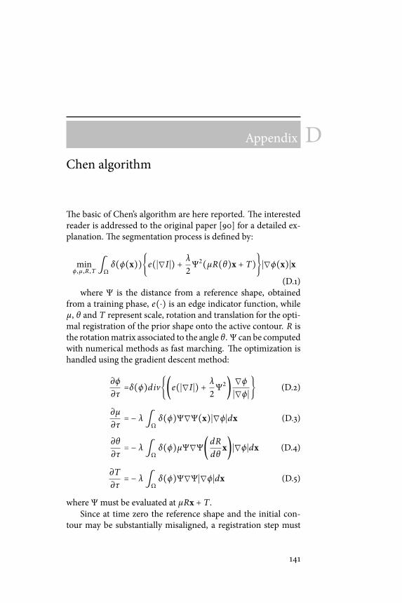
Appendix DChen algorithm
e basic of Chen’s algorithm are here reported. e interestedreader is addressed to the original paper [90] for a detailed ex-planation. e segmentation process is dened by:
minϕ ,µ ,R ,T
∫Ωδ(ϕ(x))e(∣∇I∣) + λ
2Ψ2(µR(θ)x + T)∣∇ϕ(x)∣x
(D.1)where Ψ is the distance from a reference shape, obtained
from a training phase, e(⋅) is an edge indicator function, whileµ, θ and T represent scale, rotation and translation for the opti-mal registration of the prior shape onto the active contour. R isthe rotationmatrix associated to the angle θ. Ψ can be computedwith numerical methods as fast marching. e optimization ishandled using the gradient descent method:
∂ϕ
∂τ=δ(ϕ)div(e(∣∇I∣) + λ
2Ψ2) ∇ϕ∣∇ϕ∣ (D.2)
∂µ
∂τ= − λ∫
Ωδ(ϕ)Ψ∇Ψ(x)∣∇ϕ∣dx (D.3)
∂θ
∂τ= − λ∫
Ωδ(ϕ)µΨ∇Ψ(dR
dθx)∣∇ϕ∣dx (D.4)
∂T
∂τ= − λ∫
Ωδ(ϕ)Ψ∇Ψ∣∇ϕ∣dx (D.5)
where Ψ must be evaluated at µRx + T .Since at time zero the reference shape and the initial con-
tour may be substantially misaligned, a registration step must
141

142 Chen algorithm
precede the segmentation ow. is is implemented by iteratingequations (D.3) thru (D.5) until Ψ2 reaches a minimum bound.
Weobserve that image gradient, exploited for edges location,is not a reliable indicator in low SNR situations, as in ultrasoundimages. For this reason, and for comparison purpose, we use inall the experiments the localized framework described in Sec-tion 8.1.1 as data attachment term. is implies that the le handside of (D.2) is in practice replaced by equation (8.7).

Publications list
Journal papers
[P1] T. Dietenbeck, M. Alessandrini, D. Barbosa, J. D’hooge, D.Friboulet and O. Bernard. Detection of the whole myocar-dium in echocardiography for multiple orientations usinga geometrically constrained level-set. Elsevier - MedicalImage Analysis (submitted for publication).
[P2] M. Alessandrini, S.Maggio, J. Poré e, L. DeMarchi, N. Spe-ciale, E. Franceschini, O. Bernard and O. Basset. A restor-ation framework for ultrasound tissue classication. IEEETrans. on Ultrasonics Ferroelectrics and Frequency Control(submitted for publication).
[P3] M.Alessandrini, T.Dietenbeck, O. Basset, D. Friboulet andO. Bernard. Using a geometric formulation of annular-likeshape priors for constraining variational level-sets. Elsevier- Pattern Recognition Letters (submitted for publication).
[P4] S. Maggio, A. Palladini, L. De Marchi, M. Alessandrini,N. Speciale, and G. Masetti. Predictive deconvolution andhybrid feature selection for computer-aided detection ofprostate cancer. Medical Imaging, IEEE Transactions on,29(2):455 –464, 2010.
Conference papers
[P5] S. Maggio, M. Alessandrini, N. Speciale, O. Bernard,D. Vray, O. Basset, and M. Unser. Continuous domainARMAmodeling for ultrasound tissue characterization. InProc. IEEE Trans. on International Symposium on Biomed-ical Imaging (ISBI 2011), (accepted for publication).
143

144 Publications list
[P6] T. Dietenbeck, M. Alessandrini, D. Barbosa, J. D’hooge, D.Friboulet, and O. Bernard. Multiviewmyocardial segmen-tation in echocardiographic images using a piecewise para-metric shape prior. In Proc. IEEE Trans. on InternationalSymposium on Biomedical Imaging (ISBI 2011), (acceptedfor publication)
[P7] M. Alessandrini, S. Maggio, J. Poreé, L. DeMarchi, N. Spe-ciale, E. Franceschini, O. Bernard, and O. Basset. An ex-pectationmaximization framework for an improved tissuecharacterization using ultrasounds. In Proc. of SPIE Medi-cal Imaging (2011), 2011, Orlando, USA. (accepted for pub-lication).
[P8] M. Alessandrini, T. Dietenbeck, D. Barbosa, J. D’hooge,O. Basset, N. Speciale, D. Friboulet, and O. Bernard. Seg-mentation of the fullmyocardium in echocardiography us-ing constrained level-sets. In Proc. of Computing in Cardi-ology Conference (CinC2010), pages 409–412, 26–29 Sept.2010, Belfast, Northern Ireland.
[P9] M. Alessandrini, T. Dietenbeck, O. Basset, D. Friboulet,andO. Bernard. Using a geometric formulation of annular-like shape priors for constraining variational level-sets. InImage Processing (ICIP), 2010 17th IEEE International Con-ference on, pages 669–672, 26-29 Sept. 2010, Hong Kong,China.
[P10] T. Dietenbeck, M. Alessandrini, D. Friboulet, andO. Bernard. Creaseg: a free soware for the evaluationof image segmentation algorithms based on level-sets. InImage Processing (ICIP), 2010 17th IEEE International Con-ference on, pages 665-668, 26-29 Sept. 2010, Hong Kong,China.
[P11] M. Alessandrini, D. Friboulet, O. Basset, J. D’hooge, andO. Bernard. Level-set segmentation of myocardium andepicardium in ultrasound images using localized bhat-tacharyya distance. In Ultrasonics Symposium (IUS), 2009IEEE International, pages 2468 –2471, 2009, Rome, Italy.
[P12] M. Alessandrini, A. Palladini, L.De Marchi, and N. Spe-ciale. Expectation maximization for joint deconvolutionand statistics estimation. In Proc. of International Acous-tical Imaging Symposium (AI2009), Monterey USA, 2009.(accepted for publication).

Publications list 145
[P13] M. Alessandrini, L.De Marchi, and N. Speciale. Recur-sive Least Squares adaptive lters for ultrasonic signals de-convolution. In Proc. IEEE International Symposium onCircuits and Systems (ISCAS2008), pages 2937–2940, May2008, Seattle, USA.
[P14] S. Maggio, L.De Marchi, M. Alessandrini, and N .Spe-ciale. Computer aided detection of prostate cancer basedon gda and predictive deconvolution. In Proc. IEEE In-ternational Ultrasonics Symposium (IUS2008), pages 28–31,Beijing, China, October 2008.


Bilbiography
[1] T. L. Szabo. Diagnostic Ultrasound Imaging: Inside Out.2004.
[2] Alessandro Palladini. Statistical methods for biomedicalsignal analysis and processing. PhD thesis, University ofBologna, 2009.
[3] G. D. Ludwig. e velocity of sound through tissues andthe acoustic impedance of tissues. e Journal of theAcoustical Society of America, 22:862–866, 1950.
[4] Martin E. Anderson and Gregg E. Trahey. A seminar onk-space applied to medical ultrasound, 2000.
[5] J. Jensen. Linear description of ultrasound imaging sys-tems, 2001. Notes for the International Summer Schoolon Advanced Ultrasound Imaging Technical Universityof Denmark.
[6] J.A. Jensen and N.B. Svendsen. Calculation of pressureelds from arbitrarily shaped, apodized, and excited ul-trasound transducers. IEEE Transactions on Ultrason-ics, Ferroelectrics and Frequency Control, 39(2):262 –267,March 1992.
[7] J. Ng, R. Prager, N. Kingsbury, G. Treece, and A. Gee.Modeling ultrasound imaging as a linear, shi-variantsystem. Ultrasonics, Ferroelectrics and Frequency Control,IEEE Transactions on, 53(3):549 –563, 2006.
[8] Alan V. Oppenheim, Ronald W. Schafer, and John. R.Buck. Discrete Time Digital Signal Processing. PrenticeHall, second edition, 1998.
[9] J. W. Goodman. Statistical Optics. Wiley Classic LibraryEdition, 2000.
147
148 Bilbiography
[10] P. M. Shankar, R. Molthen, V. M. Narayanan, J. M. Reid,V. Genis, F. Forsberg, C. W. Piccoli, A. E. Lindenmayer,and B. B. Goldberg. Studies on the use of non-rayleighstatistics for ultrasonic tissue characterization. Ultra-sound in Medicine & Biology, 22(7):873 – 882, 1996.
[11] V. Dutt and J. F. Greenleaf. Ultrasound echo envelopeanalysis using a homodyned k distribution signal model.Ultrasonic Imaging, 16(4):265 – 287, 1994.
[12] P. Mohana Shankar. A general statistical model for ul-trasonic backscattering from tissues. Ultrasonics, Fer-roelectrics and Frequency Control, IEEE Transactions on,47(3):727 –736, may. 2000.
[13] O. Bernard, J. D’hooge, and D. Friboulet. Statistics of theradiofrequency signal based on k distribution with appli-cation to echocardiography. IEEE Trans. Ultrason., Ferro-elect., Freq. Control, 53:1689–1694, 2006.
[14] O. Bernard, B. Touil, J. D’hooge, and D. Friboulet. Statis-tical modeling of the radio-frequency signal for partially-and fully-developed speckle based on a generalized gaus-sian model with application to echocardiography. Ultra-sonics, Ferroelectrics and Frequency Control, IEEE Trans-actions on, 54(10):2189–2194, oct. 2007.
[15] R.F. Wagner, S.W. Smith, J.M. Sandrik, and H. Lopez.Statistics of speckle in ultrasound b-scans. Sonics and Ul-trasonics, IEEE Transactions on, 30(3):156 – 163, may. 1983.
[16] StevenM. Kay. Fundamentals of Statistical Signal Process-ing, Volume I: Estimation eory (v. 1). Prentice Hall, 1edition, April 1993.
[17] A. Sarti, C. Corsi, E. Mazzini, and C. Lamberti. Maxi-mum likelihood segmentation of ultrasound images withrayleigh distribution. IEEE Trans. on Ultrasonics Ferro-electrics and FrequencyControl, 52(6):947–960, June 2005.
[18] P. M. Shankar, V. A. Dumane, C. W. Piccoli, J. M. Reid,F. Forsberg, and B. B. Goldberg. Classication of breastmasses in ultrasonic b-mode images using a compound-ing technique in the nakagami distribution domain. Ul-trasound in Medicine & Biology, 28(10):1295–1300, 2002.

Bilbiography 149
[19] Olivier Bernard. Segmentation in echocardiographic ima-ging using parametric level set model driven by the statis-tics of the radiofrequency signal. PhD thesis, University ofLyon, 2006.
[20] M. R. Spiegel and J. M. Liu. Mathematical Handbook ofFormulas and Tables. 2nd edition, 1968.
[21] M.N. Do and M. Vetterli. Wavelet-based texture re-trieval using generalized gaussian density and kullback-leibler distance. Image Processing, IEEE Transactions on,11(2):146 –158, February 2002.
[22] Patrizio Campisi & Karen Egiazarian, editor. Blind ImageDeconvolution:eory andApplications. CRCPress, 2007.
[23] SimonHaykin, editor. Blind Deconvolution. Prentice HallInformation and System Science Series. Prentice Hall,2002.
[24] E. A. Robinson. Predictive Decomposition of Time Serieswith applications to seismic exploration. PhD thesis, Mas-sachusetts Institute of Technology, 1954.
[25] J. K. Perlo. Estimation of in vivo pulses in medical ul-trasound. Ultrasonic Imaging, 16:190–203, 1994.
[26] S. Maggio, A. Palladini, L. De Marchi, M. Alessandrini,N. Speciale, andG.Masetti. Predictive deconvolution andhybrid feature selection for computer-aided detection ofprostate cancer. Medical Imaging, IEEE Transactions on,29(2):455 –464, 2010.
[27] Nicola Testoni. Adaptive Multiscale Biological Signal Pro-cessing. PhD thesis, University of Bologna, 2008.
[28] Simon Haykin. Adaptive lter theory (3rd ed.). Prentice-Hall, Inc., Upper Saddle River, NJ, USA, 1996.
[29] T. Taxt and R. Jirik. Superresolution of ultrasound imagesusing the rst and second harmonic signal. Ultrasonics,Ferroelectrics and Frequency Control, IEEE Transactionson, 51(2):163 –175, feb. 2004.
[30] T. Taxt and J. Strand. Two-dimensional noise-robustblind deconvolution of ultrasound images. Ultrasonics,Ferroelectrics and Frequency Control, IEEE Transactionson, 48(4):861 –866, jul. 2001.
150 Bilbiography
[31] O.V. Michailovich and D. Adam. A novel approach to the2-d blind deconvolution problem in medical ultrasound.Medical Imaging, IEEETransactions on, 24(1):86 –104, jan.2005.
[32] T. Taxt. ree-dimensional blind deconvolution of ultra-sound images. Ultrasonics, Ferroelectrics and FrequencyControl, IEEE Transactions on, 48(4):867 –871, 2001.
[33] J. Ng, H. Gomersall, R. Prager, N. Kingsbury, G. Treece,and A. Gee. Wavelet restoration of three-dimensionalmedical pulse-echo ultrasound datasets in an em frame-work. In Iwaki Akiyama, editor, Acoustical Imaging, vol-ume 29 of Acoustical Imaging, pages 403–408. SpringerNetherlands, 2009.
[34] Harry C. Andrews and B. R. Hunt. Digital Image Restora-tion. Prentice Hall Professional Technical Reference, 1977.
[35] J. Ng, R. Prager, N. Kingsbury, G. Treece, and A. Gee.Wavelet restoration ofmedical pulse-echo ultrasound im-ages in an em framework. Ultrasonics, Ferroelectrics andFrequency Control, IEEE Transactions on, 54(3):550 –568,2007.
[36] James Nagy and Dianne P. O’leary. Fast iterative imagerestoration with a spatially-varying psf. Technical report,1997.
[37] M.A.T. Figueiredo and R.D. Nowak. An em algorithm forwavelet-based image restoration. Image Processing, IEEETransactions on, 12(8):906 – 916, aug. 2003.
[38] J.M. Bioucas-Dias. Bayesian wavelet-based image decon-volution: a gem algorithm exploiting a class of heavy-tailed priors. Image Processing, IEEE Transactions on,15(4):937 –951, apr. 2006.
[39] Jonathan Richard Shewchuk. An introduction to the con-jugate gradientmethodwithout the agonizing pain. Tech-nical report, 1994.
[40] T. Taxt and G.V. Frolova. Noise robust one-dimensionalblind deconvolution ofmedical ultrasound images.Ultra-sonics, Ferroelectrics and Frequency Control, IEEE Trans-actions on, 46(2):291 –299, mar. 1999.

Bilbiography 151
[41] James Kee Huat Ng. Restoration of medical pulse echoultrasound images. Technical report, 2006.
[42] S. Boyd and L. Vandenberghe. Convex Optimization.2004.
[43] O. Michailovich and A. Tannenbaum. Blind deconvolu-tion of medical ultrasound images: A parametric inverseltering approach. Image Processing, IEEE Transactionson, 16(12):3005 –3019, dec. 2007.
[44] U.R. Abeyratne, A.P. Petropulu, and J.M. Reid. Higherorder spectra based deconvolution of ultrasound images.Ultrasonics, Ferroelectrics and Frequency Control, IEEETransactions on, 42(6):1064 –1075, November 1995.
[45] O.Michailovich andD.Adam. Robust estimation of ultra-sound pulses using outlier-resistant de-noising. MedicalImaging, IEEE Transactions on, 22(3):368 –381, mar. 2003.
[46] R. Jiric and T. Taxt. High-resolution ultrasonic ima-ging using fast two-dimensional homomorphic ltering.Ultrasonics, Ferroelectrics and Frequency Control, IEEETransactions on, 53(8):1440–1448, 2006.
[47] Dennis C. Ghiglia and Mark D. Pritt. Two-DimensionalPhase Unwrapping:eory, Algorithms, and Soware. Wi-ley, 1998.
[48] C. L. Nikias and A. P. Petropulu. Higher Order SpectralAnalysis: A Nonlinear Signal Processing Framework. Pren-tice Hall, 1993.
[49] O.V.Michailovich andD.Adam. Phase unwrapping for 2dblind deconvolution of ultrasound images. Medical Ima-ging, IEEE Transactions on, 23(1):7 –25, jan. 2004.
[50] T. Taxt. Restoration of medical ultrasound images usingtwo-dimensional homomorphic deconvolution. Ultra-sonics, Ferroelectrics and Frequency Control, IEEE Trans-actions on, 42(4):543 –554, July 1995.
[51] T. Taxt. Comparison of cepstrum-based methods for ra-dial blind deconvolution of. ultrasound images. Ultra-sonics, Ferroelectrics and Frequency Control, IEEE Trans-actions on, 44(3):666 –674, May 1997.

152 Bilbiography
[52] J. Strand and T. Taxt. Two-dimensional phase un-wrapping using robust derivative estimation and adap-tive integration. Image Processing, IEEE Transactions on,11(10):1192 – 1200, October 2002.
[53] Jarle Strand and Tornn Taxt. Performance evaluationof two-dimensional phase unwrapping algorithms. Appl.Opt., 38(20):4333–4344, Jul 1999.
[54] Oleg Michailovich and Allen Tannenbaum. On approx-imation of smooth functions from samples of partialderivatives with application to phase unwrapping. SignalProcessing, 88(2):358 – 374, 2008.
[55] Dennis C. Ghiglia and Louis A. Romero. Robust two-dimensional weighted and unweighted phase unwrap-ping that uses fast transforms and iterative methods. J.Opt. Soc. Am. A, 11(1):107–117, Jan 1994.
[56] S. Maggio, M. Alessandrini, L. De Marchi, and N. Spe-ciale. Computer aided detection of prostate cancer basedon gda and predictive deconvolution. InUltrasonics Sym-posium, 2008. IUS 2008. IEEE, pages 28 –31, 2008.
[57] Mehdi Moradi, Parvin Mousavi, and Purang Abolmae-sumi. Computer-aided diagnosis of prostate cancer withemphasis on ultrasound-based approaches: A review. Ul-trasound in Medicine & Biology, 33(7):1010 – 1028, 2007.
[58] D. Fukuoka, Y. Ikedo, T. Hara, H. Fujita, E. Takada,T. Endo, andT.Morita. Development of breast ultrasoundcad system for screening. Lecture Notes in Computer Sci-ence, pages 392–?398, September 2006.
[59] J.M. ijssen, A. Starke, G. Weijers, A. Haudum,K. Herzog, P. Wohlsein, J. Rehage, and C.L. De Korte.Computer-aided b-mode ultrasound diagnosis of hepaticsteatosis: a feasibility study. Ultrasonics, Ferroelectrics andFrequencyControl, IEEETransactions on, 55(6):1343 –1354,jun. 2008.
[60] Frederic L. Lizzi, Michael Greenebaum, Ernest J. Feleppa,Marek Elbaum, and D. Jackson Coleman. eoreti-cal framework for spectrum analysis in ultrasonic tissuecharacterization. e Journal of the Acoustical Society ofAmerica, 73(4):1366–1373, 1983.

Bilbiography 153
[61] T. Liu, F. L. Lizzi, J. A. Ketterling, R. H. Silverman, andG. J. Kutcher. Ultrasonic tissue characterization via 2-d spectrum analysis: eory and in vitro measurements.Medical Physics, 3(34):1037–1046, March 2007.
[62] Frederic L. Lizzi, Ernest J. Feleppa, S. Kaisar Alam, andCheri X. Deng. Ultrasonic spectrum analysis for tissueevaluation. Pattern Recognition Letters, 24(4-5):637 – 658,2003.
[63] O. Basset, Z. Sun, JL. Mestas, and G. Gimenez. Textureanalysis of ultrasonic images of the prostate by means ofco-occurrence matrices. Ultrason Imaging, 15(3):218–237,July 1993.
[64] Chung-Ming Wu, Yung-Chang Chen, and Kai-ShengHsieh. Texture features for classication of ultrasonicliver images. Medical Imaging, IEEE Transactions on,11(2):141 –152, jun. 1992.
[65] F. Rakebrandt, D. C. Crawford, D. Havard, D. Coleman,and J. P.Woodcock. Relationship between ultrasound tex-ture classication images and histology of atheroscleroticplaque. Ultrasound in Medicine & Biology, 26(9):1393–1402, 2000.
[66] P. H. Tsui, C. C. Huang, and S. H. Wang. Use of nak-agami distribution and logarithmic compression in ultra-sonic tissue characterization. Journal of Medical and Bio-logical Engineering, 26(2):69–73, May 2006.
[67] D. Donoho. On minimum entropy deconvolution. Tech-nical report, 1981.
[68] A. P. Dempster, N. M. Laird, and D. B. Rubin. Maximumlikelihood from incomplete data via the em algorithm.Journal of the Royal Statistical Society. Series B (Method-ological), 39(1):1–38, 1977.
[69] Timothy E. Doyle, Adam T. Tew, Keith H. Warnick, andBrent L. Carruth. Simulation of elastic wave scattering incells and tissues at the microscopic level. e Journal ofthe Acoustical Society of America, 125(3):1751–1767, 2009.
[70] A. R. Webb. Statistical Pattern Recognition. 2nd edition.
154 Bilbiography
[71] Statistical pattern recognition tool-box (stprtool). online available at:http://cmp.felk.cvut.cz/cmp/cmp_software.html.
[72] Roxana M. Vlad, Ratan K. Saha, NehadM. Alajez, ShawnRanieri, Gregory J. Czarnota, and Michael C. Kolios. Anincrease in cellular size variance contributes to the in-crease in ultrasound backscatter during cell death. Ul-trasound in Medicine & Biology, 36(9):1546 – 1558, 2010.
[73] M.L. Oelze, Jr. O’Brien, W.D., J.P. Blue, and J.F. Zachary.Dierentiation and characterization of rat mammary -broadenomas and 4t1 mouse carcinomas using quantita-tive ultrasound imaging. Medical Imaging, IEEE Transac-tions on, 23(6):764 –771, jun. 2004.
[74] Department of Public Health. European cardiovascu-lar disease statistics, 2008 edition. online available at:http://www.heartstats.org/datapage.asp?id=7683.
[75] M. Alessandrini, D. Friboulet, O. Basset, J. D’hooge, andO. Bernard. Level-set segmentation of myocardium andepicardium in ultrasound images using localized bhat-tacharyya distance. InUltrasonics Symposium (IUS), 2009IEEE International, pages 2468 –2471, 2009.
[76] M. Alessandrini, T. Dietenbeck, O. Basset, D. Friboulet,and O. Bernard. Using a geometric formulation ofannular-like shape priors for constraining variationallevel-sets. In Proc. IEEE International Conference on Im-age Processing (ICIP2010), pages 669–672, Hong Kong,2010.
[77] M. Alessandrini, T. Dietenbeck, D. Barbosa, J. D’hooge,O. Basset, N. Speciale, D. Friboulet, and O. Bernard. Seg-mentation of the full myocardium in echocardiographyusing constrained level-sets. InProc. of Computing in Car-diology Conference (CinC2010), Belfast, Northern Ireland,September 2010. accepted for publication.
[78] M. Alessandrini, T. Dietenbeck, O. Basset, D. Friboulet,and O. Bernard. Using a geometric formulation ofannular-like shape priors for constraining variationallevel-sets. Pattern Recognition Letters. submitted for pub-lication.
Bilbiography 155
[79] M. Kass, A. Witkin, and D. Terzopoulos. Snakes: Activecontour models. International Journal of Computer Vi-sion, 1(4):321–331, 1988.
[80] Stanley J. Osher and Ronald P. Fedkiw. Level Set Methodsand Dynamic Implicit Surfaces. Springer, 2002.
[81] R. Malladi, J.A. Sethian, and B.C. Vemuri. Shape model-ing with front propagation: a level set approach. PatternAnalysis and Machine Intelligence, IEEE Transactions on,17(2):158 –175, feb. 1995.
[82] Xavier Bresson. Image Segmentation with Variational Ac-tive Contours. PhD thesis, Ecole Politechnique Federalede Lausanne, 2005.
[83] S.C. Zhu, T.S. Lee, and A.L. Yuille. Region competition:unifying snakes, region growing, energy/bayes/mdl formulti-band image segmentation. pages 416 –423, jun.1995.
[84] T. F. Chan and L. A. Vese. Active contours without edges.IEEE Trans. on Image Processing, 10(2):266–277, February2001.
[85] S. Lankton and A. Tannenbaum. Localizing region-basedactive contours. IEEE Trans. on IP, 17(11):2029–2039,2008.
[86] D. Cremers, M. Rousson, and R. Deriche. A review of sta-tistical approaches to level set segmentation: Integratingcolor, texture, motion and shape. International Journal onComputer Vision, 2(72):195–215, 2007.
[87] O. Michailovich, Y. Rathi, and A. Tannenbaum. Imagesegmentation using active contours driven by the bhat-tacharyya gradient ow. IEEE Trans. on Image Processing,16(11):2787–2801, November 2007.
[88] StevenM. Kay. Fundamentals of Statistical Signal Process-ing: Estimationeory. Prentice Hall, 1993.
[89] T. Chan and Wei Zhu. Level set based shape prior seg-mentation. In Computer Vision and Pattern Recognition,2005. CVPR 2005. IEEE Computer Society Conference on,volume 2, pages 1164 – 1170 vol. 2, 2005.

156 Bilbiography
[90] Yunmei Chen, Hemant D. Tagare, Sheshadri iru-venkadam, Feng Huang, David Wilson, Kaundinya S.Gopinath, Richard W. Briggs, and Edward A. Geiser. Us-ing prior shapes in geometric active contours in a varia-tional framework. Int. J. Comput. Vision, 50:315–328, De-cember 2002.
[91] Mikael Rousson and Nikos Paragios. Shape priors forlevel set representations. In In Proc. ECCV, pages 78–92.Springer, 2002.
[92] X. M. Pardo, V. Leborán, and R. Dosil. Integrating priorshape models into level-set approaches. Pattern Recogni-tion Letters, 25(6):631–639, 2004.
[93] M. E. Leventon, W. Eric, L. Grimson, and O. Faugeras.Statistical shape inuence in geodesic active contours. InComputer Vision and Pattern Recognition, 2000. CVPR2000. IEEE Computer Society Conference on, volume 1,page 1316, 2000.
[94] E. D. Folland, A. F. Parisi, P. F. Moyniham, D. R. Jones,C. L. Feldman, and D. E. Tow. Assessment of le-ventricular ejection fraction and volumes by real-timetwo-dimensional echocardiography: A comparison ofcineangiographic and radionuclide techniques. Circula-tions, 66:760 –766, 1979.
[95] D. A. Conetta, E. A. Geiser, L. H. Olivier, A. B. Miller, andR.Conti. Reproducibility of le-ventricular area and vol-ume measurements using a computer endocardial edgedetection algorithm in normal subjects. Amer. J. Cardiol,56:947–952, 1985.
[96] J.A.Noble andD. Boukerroui. Ultrasound image segmen-tation: a survey. Medical Imaging, IEEE Transactions on,25(8):987 –1010, aug. 2006.
[97] J. K. Perlo. Development and regression of increasedventricular mass. Am J Cardiol., 50(3):605–611, 1982.
[98] J.M.B. Dias and J.M.N. Leitao. Wall position and thick-ness estimation from sequences of echocardiographic im-ages. Medical Imaging, IEEE Transactions on, 15(1):25 –38,feb. 1996.

Bilbiography 157
[99] V. Chalana, D.T. Linker, D.R. Haynor, and Yongmin Kim.Amultiple active contourmodel for cardiac boundary de-tection on echocardiographic sequences. Medical Ima-ging, IEEE Transactions on, 15(3):290 –298, jun. 1996.
[100] S. Kamaledin Setarehdan and John J. Soraghan. Au-tomatic cardiac lv boundary detection and tracking us-ing hybrid fuzzy temporal and fuzzy multiscale edge de-tection. Biomedical Engineering, IEEE Transactions on,46(11):1364 –1378, nov. 1999.
[101] C.H. Chu, E.J. Delp, and A.J. Buda. Detecting le ven-tricular endocardial and epicardial boundaries by digi-tal two-dimensional echocardiography. Medical Imaging,IEEE Transactions on, 7(2):81 –90, jun. 1988.
[102] Maxime Taron, Nikos Paragios, and Marie-Pierre Jolly.Border detection on short axis echocardiographic viewsusing a region based ellipse-driven framework. In Med-ical Image Computing and Computer-Assisted Interven-tion MICCAI 2004, volume 3216 of Lecture Notes in Com-puter Science, pages 443–450. Springer Berlin / Heidel-berg, 2004.
[103] J. M. Berg. On parameter estimation using level sets.SIAM Journal on Control and Optimization, 37:1372–1393,1998.
[104] A. Fitzgibbon,M. Pilu, andR.B. Fisher. Direct least squaretting of ellipses. Pattern Analysis and Machine Intelli-gence, IEEE Transactions on, 21(5):476 –480, may. 1999.
[105] Petko Faber andR.B. Fisher. Euclidean tting revisited. InCarlo Arcelli, Luigi Cordella, and Gabriella Di Baja, edi-tors, Visual Form 2001, volume 2059 of Lecture Notes inComputer Science, pages 165–175. Springer Berlin / Hei-delberg, 2001.
[106] Sung Joon Ahn, Wolfgang Rauh, and Hans-J?rgen War-necke. Least-squares orthogonal distances tting of circle,sphere, ellipse, hyperbola, and parabola. Pattern Recogni-tion, 34(12):2283 – 2303, 2001.
[107] V. Caselles, R. Kimmel, and G. Sapiro. Geodesic ac-tive contours. International Journal on Computer Vision,22:61–79, 1995.

158 Bilbiography
[108] GeneH.Golub andCharles F. Van Loan.Matrix computa-tions (3rd ed.). JohnsHopkinsUniversity Press, Baltimore,MD, USA, 1996.
[109] T. Dietenbeck, M. Alessandrini, D. Barbosa, J. D’hooge,D. Friboulet, and O. Bernard. Multiview myocardial seg-mentation in echocardiographic images using a piecewiseparametric shape prior. In In Proc. IEEE Trans. on Inter-national Symposium on Biomedical Imaging (ISBI 2011),2011. submitted for publication.
[110] Yun Zhu, Xenophon Papademetris, Albert J. Sinusas, andJames S. Duncan. A coupled deformable model for track-ing myocardial borders from real-time echocardiographyusing an incompressibility constraint. Medical ImageAnalysis, 14(3):429 – 448, 2010.
[111] V. Chalana and Y. Kim. A methodology for evaluation ofboundary detection algorithms on medical images. Med-ical Imaging, IEEE Transactions on, 16(5):642 – 652, Octo-ber 1997.
[112] D.P. Huttenlocher, G.A. Klanderman, and W.A. Ruck-lidge. Comparing images using the hausdor distance.IEEE Transactions on Pattern Analysis and Machine Intel-ligence, 15:850–863, 1993.
[113] James G. Nagy and Dianne P. O’Leary. Restoring imagesdegraded by spatially variant blur. SIAM J. Sci. Comput.,19:1063–1082, July 1998.


Martino Alessandrini was born in Bologna, Italy, in 1983. Heobtained a B.Sc. degree in Electronic Engineering in 2005 anda M.Sc. degree in Electronic Engineering for Biomedical Ap-plications in 2007, both at the Università di Bologna. He wasawarded the Ph.D. degree from the same university in 2011, witha thesis concerning deconvolution and segmentation of medicalultrasound images. His main research interests are in the ledof image and signal processing and include solution of ill con-ditioned problems, variational techniques for image segmenta-tion, restoration and denoising, multi-resolution analysis, sta-tistical estimation theory and adaptive ltering.


![Economic Concrete Bridge Design 15-45m - 3482-52-04[1]](https://static.fdocuments.in/doc/165x107/577cdfa71a28ab9e78b1b2c1/economic-concrete-bridge-design-15-45m-3482-52-041.jpg)


