Statistical techniques in music psychology: An

update

Daniel Mullensiefen

1 Introduction

Music psychology as a discipline has its origins at the end of the 19th centuryand ever since then, empirical methods have been a core part in this field ofresearch. While its experimental and analytical methods have mainly been relatedto methodology employed in general psychology, several statistical techniques haveemerged over the course of the past century being specific for empirical researchin music psychology. These core methods have been described in a few didacticand summarising publications at several stages of the discipline’s history (see e.g.Wundt, 1882; Bottcher & Kerner, 1978; Windsor, 2001, or Beran, 2004 for avery technical overview), and these publications have been valuable resources tostudents and researchers alike. In contrast to these texts with a rather didacticalfocus, the objective of this chapter is to provide an overview of a range of novelstatistical techniques that have been employed in recent years in music psychologyresearch.1 This overview will give enough insight into each technique as such. Theinterested reader will then have to turn to the original publications, to obtain amore in-depth knowledge of the details related to maths and the field of application.

Empirical research into auditory perception and the psychology of music mighthave its beginnings in the opening of the psychological laboratory by WilhelmWundt in Leipzig in 1879 where experiments on human perception were conducted,and standards for empirical research and analysis were developed. From the earlystages until today, the psychology of music followed largely the topics and trends of

1This paper has also been inspired by conversations with Albrecht Schneider in the context ofjointly taught seminars on Advanced Statistical Techniques in Music Psychology at the HamburgInstitute of Musicology. On these occasions, Albrecht Schneider repeatedly mentioned that itwas about time to write an update of the standard textbook Methoden in der Musikpsychologie

by Bottcher and Kerner (1978). While this paper can hardly be considered a didactical textnor does it describe a firm canon of modern and frequently methods in music psychology, it stillmight convey an impression of how such an update might look like (if one actually was to writeone).

1

general psychology, each time with a considerable time lag, including psychophysics(psychoacoustics), Gestalt psychology, individual differences, cognitive psychology,and computer modelling. Each field of research is associated with a canon ofempirical and statistical methods which are shared among the research community.

In this chapter we will highlight a few selected statistical methods used inmore recent empirical studies which might indicate new trends for the analysisof psycho-musicological data. We focus on two fields of research: first, cognitivemusic psychology, and second, computer models of musical structure with psycho-logical constraints and mechanisms as core parts of the models. The distinctionbetween these two areas is somewhat arbitrary, and is made on the pragmaticgrounds that studies in the cognitive psychology of music mainly aim at explain-ing experimental data from human subjects whereas in computer modelling themusic itself is taken as the data that is to be explained. Due to space limitationswe will not cover adjacent areas such as the neurosciences of music, music infor-mation retrieval, or individual differences (including tests of musical ability). Asan engineering science, music information retrieval (e.g. Orio, 2006) has devel-oped a vast arsenal of sophisticated statistical and machine learning techniques,although it has been lamented (e.g. Flexer, 2006) that proper statistical evaluationof algorithms and techniques is often under-represented in this field. Individualdifferences and personality psychology naturally have a strong connection to testconstruction and measurement theory, while methods of statistical evaluation inthe neuropsychology of music tend to be similar to those in cognitive music psy-chology, and thus can be considered as being partly covered in this short review.Inspired by neuroscience research is the deployment of artificial neural networksto model cognitive music systems or experimental data. However, the large bodyof literature describing the use of artificial neural networks in music psychology(see Bharucha, 1987; Desain & Honing, 1992; Tillmann et al., 2003) is beyond thescope of this review.

2 Cognitive psychology of music

2.1 The standard repertoire

Cognitive psychology of music traditionally explains music perception and musicrelated behaviour in terms of mental mechanisms and concepts, such as memory,affects, mental processes, and mental representations. While mental mechanismsand concepts are usually unobservable, it is possible to generate hypotheses aboutempirically evident phenomena from the assumptions and specifications that thecognitive concepts imply. Therefore, a large amount of empirical work uses infer-ential statistics to test the validity of cognitive models and their parameters. Stan-

2

dard techniques comprise procedures for univariate comparisons between groups,mainly in their parametric version (uni- and multi-factorial ANOVAs, t-test etc.)and, to a lesser degree, include also robust techniques such as rank-based tests.For relating one dependent to several independent variables on an interval levelof measurement, linear regression is a popular statistical method (e.g. Eerola etal., 2002; Cuddy & Lunney, 1995), although rigorous evaluation of the predictivepower of the resulting regression models is seldom undertaken. Bivariate cor-relation, frequency association measures (χ2), and descriptive statistics are alsocommonly employed to arrive at an understanding of the relationships betweena number of predictors and one dependent variable (a simultaneous analysis ofseveral dependent variables is possible but unusual).

In summary, the main concern of a large number of empirical psychomusicolog-ical studies is to identify one or more important (i.e. significant) determinants forcognitive behaviour as measured by a dependent variable. However, the amountof noise in the linear model is usually of less concern. That is, low R2 values inregression models are not really a matter of concern, and generally little thoughtis invested in alternative loss functions or measures of model accuracy. Thus, thefocus has been mainly on hypothesis testing rather than on statistical modelling.The beneficial side of this ‘statistical conservatism’ in music psychology is thatexperimental data and results can be easily compared, exchanged, and replicated.But at the same time, the reluctance to explore the variety of statistical modellingtechniques available nowadays for many specific analysis situations, might leave in-teresting information in some experimental datasets uncovered. A review of thesequasi-canonical methods directed at music researchers can be found in Windsor(2001).

For exploratory purposes, data reduction and scaling techniques, such as prin-cipal component analysis and multi-dimensional scaling (MDS), have frequentlybeen used in music cognition studies. Examples include the semantic differential asa technique of data collection along with subsequent factor analysis introduced toGerman music psychology by Reinecke in the 1960s (see Bottcher & Kerner, 1978,for an overview). Principal component analysis has also been used more recentlyto simplify cognitive models, such as models for melodic expectation (Schellenberg,1997).

2.2 Current models of multidimensional scaling

Multidimensional scaling has mainly been used as a means to reveal and visualiseunobservable cognitive or judgemental dimensions that are of importance in aspecific domain, such as tonal or harmonic relationships (Krumhansl & Kessler,1982; Bharucha & Krumhansl, 1983), timbre similarity (Kendall & Carterette,1991, Markuse & Schneider, 1996), or stylistic judgements (Gromko, 1993). In

3

general, experiments start from similarity judgements that N subjects make aboutPJ =

(

n

2

)

unordered pairs out of J auditory stimuli and aim at positioning theJ auditory stimuli in a low-dimensional space with R dimensions where R �P . The R dimensions are then often interpreted as perceptual dimensions thatgovern human similarity perception and categorisation. Classical MDS algorithmsposition the judged objects in an Euclidean space where the distance, djj′ betweenthe stimuli j and j′ is given by

djj′ =

[

R∑

r=1

(xjr − xj′r)2

]

1

2

where xjr is the coordinate of musical stimulus j on the (perceptual) dimension r.Since the Euclidean model cannot reflect differences between different sources ofjudgements, subjects’ individual judgements are often aggregated before classicalMDS solutions are computed. To accommodate individual differences betweensubjects, Carroll and Chang (1970) proposed the INDSCAL model where a weightwnr is introduced that reflects the importance of the perceptual dimension r forsubject n (n = 1, · · · , N)

djj′ =

[

R∑

r=1

wnr(xjr − xj′r)2

]

1

2

with wnr ≥ 0.The INDSCAL model removes rotational invariance and makes the MDS model

easier to interpret since the potentially many rotational variants of a given modeldo not have to be considered for interpretation any more. In turn, it generatesN × R weight parameters wnr for every combination of subjects and dimensions.However, these parameters are only of marginal interest if the goal of the inves-tigation is to discover perceptual dimensions that are generalisable to a largerpopulation of listeners. A very interesting extension of the classical MDS modelwas proposed by Winsberg and De Soete (1993), labelled CLASCAL. In CLAS-CAL models, the numerous separate parameters for every combination of subjectand dimension, are replaced by so-called latent classes T which reflect types ofsubjects’ judgemental behaviour. Since the number of latent classes is assumed tobe much lower than the number of subjects N , considerably fewer weights wtr forthe combinations of dimensions and latent classes have to be estimated than inthe INDSCAL model. The CLASCAL model by Winsberg and De Soete (1993) isgiven by

4

djj′t =

[

R∑

r=1

wtr(xjr − xj′r)2

]

1

2

where wtr is the weight for the latent class t with respect to dimension r. Theconcept of latent classes that group together subjects with similar judgemental be-haviour can potentially be very useful for future research in music psychology whenresearchers want to explicitly allow for the possibility that subjects perceive andjudge musical stimuli differently, but where a notion of wrong or right perceptionsor judgements does not apply. Divergent judgements of musical or aesthetic ob-jects in general might be caused by differences in subjects’ musical backgrounds,their degree of specialisation and familiarisation with certain musical styles, orsimply by their taste.2

The latent class approach seems to be a good compromise between the re-ductionist approach of just considering the mean of human judgements on theone hand, and models that require one or more parameter value for each subject(e.g. the INDSCAL model) on the other hand, yielding results that are hard togeneralise. The latent class approach is also consistent with the general assump-tion that there are equally valid but substantially different ways to judge musicalobjects that, however, for a homogeneous population of listeners are limited innumber. For demonstration purposes, we turn to timbre perception as the studyarea. Here, a number of publications make use of an extended CLASCAL modelas the statistical method. The extended model is given by

djj′t =

[

R∑

r=1

wtr(xjr − xj′r)2 + νt(sj + sj′)

]

1

2

where sj and sj′ are coordinates on dimensions that are specific to the objectsj and j′, i.e. not shared with other objects. The parameter νt is the weight alatent class gives to the whole set of specific dimensions. It reflects how much aperceptual strategy uses common and general perceptual dimensions to comparemusical objects or how much it attends to the specificities of each musical stimulus.McAdams, Winsberg, Donnadieu, De Soete, and Krimphoff (1995) applied this ex-tended CLASCAL model to 153 pairwise comparisons of 18 instrument timbres asobtained from judgments by 88 subjects with different degrees of musical training.The authors found five different latent classes of judgmental behaviour and ob-tained a three-dimensional model with instrument-specific dimensions. These fivelatent classes were only very partially explained by the amount of musical training

2It is not surprising that latent class models have been quite popular in food science wheresubjects’ judgements in sensometric experiments are usually not regarded as being right or wrongbut simply as different from one another (Sahmer, Vigneau, & Qannari, 2006)

5

subjects had received. Instead it seems likely, that the latent classes reflect dif-ferent judgemental behaviour in terms of the perceptual dimensions attended to.McAdams et al. (1995) were able to correlate the three dimensions of their modelvery closely with three different acoustic parameters previously investigated byKrimphoff, McAdams, and Winsberg (1994), namely log-attack time, the spectralcentroid, and spectral flux. They also suggested some distinguishing character-istics that could be aligned to the specificities of each instrument, for examplethe hollow timbre of the clarinet or the very sharp, pinched offset with clunk ofthe harpsichord. These examples show the point of employing an MDS model tospecificities: The sharp pinched sound of a harpsichord is only at a very abstractlevel comparable to the hollow timbre of a clarinet, but when the clunk is presentin a sound it can be a very important factor for timbre perception. A more recentstudy by Caclin, McAdams, Smith, and Winsberg (2005), employing the recentCONSCAL model, confirmed the close relations between perceptual dimensionsand attack time, spectral centroid, and spectral flux, and also discovered the sig-nificant role of the attenuation of even harmonics. The work on scaling techniquesand their application to timbre perception is on-going (see Burgoyne & McAdams,2007), and it might generate some interesting results on individual perceptualdifferences between different groups of subjects along with models describing thedifferent perceptual strategies.

2.3 Classification and regression trees

For a long time classification and regression trees have been part of the tools andtechniques for general data mining and machine learning. However, there havebeen only a few studies in music psychology that make use of the inherent advan-tages of these models as we shall see below. Although various software packagesfor statistical computing (SPSS, SAS, Statistica, R) have implemented several dif-ferent but related models and algorithms (e.g. CHAID, ID3, C4.5, CART), wejust take two studies as examples that both make use of the CART algorithm asimplemented in R.

Classification and regression trees partition observations into categories alonga dependent variable y by using the information in the set of independent variablesX. The goal is to arrive at a robust model that enables us to predict the valueof y given the values for X in a future case. Tree models belong to the areaof supervised learning which means that they learn from complete datasets thatcontain a sufficiently large number of cases with given values for y and X. Themodels are visualised in a very straight-forward manner as tree structures wherenodes represent subsets of the original dataset and branches lead from one subset ofthe data to two subsets at the next lower level. The first node contains the originaldataset. It is called root, and the algorithm starts here by recursively partitioning

6

the dataset into smaller and smaller subsets. Figure 1 gives an example of thevisualisation of a tree model. The example is taken from a recent study on melodicaccent perception (?, ?) where tree models are employed to predict the perceptualaccent strengths of individual notes in a melody on the basis of a large set of rules,mainly derived from Gestalt laws.

For the construction of a classification or regression tree one has to decide onthree questions (see Breiman et al., 1984):

1. When and how should a node be split into two subnodes?

2. When is a node an end node that should not be split any further? In otherwords, how should the size and complexity of the tree be determined?

3. How should the end nodes (leaves) be labelled, i.e. how does the tree makepredictions?

The first two questions rely on measures of the classification or regression ac-curacy of the tree as a whole. They decide on the question whether or not theclassification accuracy of the dataset as a whole is better if a node is split into twosubnodes. For classification trees where the dependent variable y is categorical,the Gini-Index is a widely used measure. It is defined as

I(t) =∑

j 6=i

p(i|t)p(j|t)

where I(t) denotes the impurity of the observations in a node and p(i|t) is theprobability for a random observation t to be assigned to class i. By recursivelysplitting the tree into subbranches, the algorithm seeks to minimise the Gini-Index.For interval-scale-dependent variables, the so-called ANOVA criterion is generallyemployed for splitting a node. This criterion is defined as SSK−(SSL+SSR) whereSSK =

∑

(yi− y)2 and SSL and SSR are the sum of the squared differences in theleft and right subnode. The ANOVA criterion is sought to be maximised in such away that at each node with each independent variable x the partitioning algorithmtests whether the accuracy criterion can be improved by splitting the data intotwo subnodes according to all potential values of x. Where the improvement in thecriterion is largest, the value of x is then chosen as the splitting or decision value.The recursive partitioning into smaller and smaller subnodes is carried out untilthe endnodes (leaves) only contain a minimal number of observations. However,in order to generate a stable tree that is not overfitted on the learning dataset, thefull tree has to be pruned subsequently. In other words, only true relations betweendependent and independent variables should be reflected in the tree model. Thisis achieved by using the so-called cross-validation method. Cross-validation uses

7

Figure 1: Regression tree model from Mullensiefen et al. (under review). Thegraph reads from top to bottom. Observations (here: notes of a melody) arerecursively partitioned into smaller subsets by binary splits at each node. Allobservations satisfying the splitting criterion (i.e. answering ‘yes’ to question inbox) are gathered together in the child node to the right and all observationsnot satisfying the condition form the subset represented by the child node to theleft. The end nodes at the bottom of the graph contain prediction values (here:perceptual accent strength on a scale from 0 to 1) for all observations classified bythe sequence of binary conditions in the same way, from the root to the end node.

8

the information from a larger portion of the data to build a tree model which thenpredicts the observations of a smaller data subset. The classification error of thecross-validated tree model is usually getting smaller as the tree model increases incomplexity (i.e. it has more nodes). However, from a certain degree of complexity,the cross-validation error arrives at a plateau or even increases with increasingcomplexity. Therefore, Therneau and Atkinson (1997) suggest a good balancebetween partitioning accuracy and tree complexity so that tree stability is reachedwhen the cross-validation error has reached its plateau.

As an example, Mullensiefen and Hennig (2006) use classification and regres-sion trees among other techniques from the data mining repertory (including ran-dom forests, linear and ordinal regression, and k -nearest neighbour) to explain theparticipants’ responses in a music memory task. The task consisted of spottingdifferences between a target melody in its musical context and an isolated com-parison melody, similar or identical to the context melody. The study aimed atidentifying the factors that determine recognition memory for new melodies andtunes (see also exp. 2 from Mullensiefen, 2004). As the most important predictorsfor explaining these memory recognition judgements, the overall melodic similar-ity, and the similarity of the melodic accent structures, as well as the subjects’musical activity were identified.

Another example for the application of classification and regression trees is astudy by Kopiez, Weihs, Ligges, and Lee (2006) where the authors try to predictperformance in a sight reading task. The predictor (independent) variables in thisstudy include general and elementary cognitive skills as measured by standardpsychological tests, as well as practice-related skills and the amount of time in-vested in musical activities. For classifying 52 subjects into good and bad sightreaders, linear discriminant analysis gave slightly better results than a classifica-tion tree from the CART family. Among the most important factors to predicthigh achievements in the sight reading task were the subjects’ speed at playingtrills, their mental speed as measured by a number connection test, and the timeinvested in sight reading before the age of 15.

Taken together, both application examples show that classification and regres-sion trees are only one out of a larger number of statistical techniques that maybe used as classification or prediction models, although tree models might notnecessarily deliver the most accurate prediction results. Nonetheless, they havea few particular advantages that seem to fit circumstances well in many musicpsychology experiments. Among these advantages are:

1. If many independent variables can be assumed to influence the dependentvariable under study, selection mechanisms become quite important to iden-tify the variables with most explanatory power. Two mechanisms alreadybuilt into tree models serve this need for variable selection., which are, first,

9

recursive partitioning by the variables that provide the largest increase inthe accuracy criterion, and second, tree pruning as such.

2. In data sets from music psychology experiments, predictor variables (e.g.variables on musical background) often have missing values for some ob-servations (subjects), and the concept of surrogate predictor variables (notexplained here due to space limitations) copes easily with these cases.

3. In many cases, higher-order interactions between several predictor variablescannot be ruled out from the model a priori. Tree models represent theseinteraction terms very effectively. In fact, tree models might be regarded asmodels of variable interactions only, mainly ignoring additive effects that arebetter modelled by linear models.

4. Non-linear relationships between the dependent and one or more independentvariables can be accommodated for in tree models, while linear models, bydefinition, are rather poor at modelling non-linear relationships.

5. Tree models make only few assumptions regarding the distribution of thedata which is in contrast to many linear models that rely, for example, onthe normal distribution of the residuals.

6. The option to visualise tree models as graphs that even non-scientists canunderstand by intuition, yields the potential to popularise and communicateresearch results beyond a circle of experts.

It quite likely that these advantages make tree models an attractive tool formusic psychologists in the future, especially in comparison with linear models thatare currently by far more popular in this study area.

2.4 Functional data analysis

Given that music is a time-dependent domain and music cognition presumablyevolves in time as well, it is surprising how few studies in the field of music cognitionmake explicit use of time related information in their statistical analysis (for anotable exception see the study of continuous emotional responses during musiclistening based on time series analysis by Schubert and Dunsmuir (1999)).

Functional data analysis (FDA) is a relatively new statistical concept thatis particularly well-suited to represent and analyse how musical parameters orobserved human reactions to music evolve over time. A functional datum is nota single observation but a set of measurements along the time axis that can beregarded as a single entity (see Levitin et al., 2007). This means that in FDA,observations are curves of random functions and not values of random variables.

10

Even though data are only sampled at discrete interval steps along a continuum,the aim of FDA is to express the variation in the variable of interest as a functionof a continuous variable, most commonly time. Thus, FDA provides the ability toquantify the dynamics of the variable under study.

A typical FDA runs through a series of steps which we here describe very brieflyfollowing the detailed explanations in Ramsay and Silverman (2005); Levitin et al.(2007).

1. Data gathering The raw values of the dependent variable yj are recordedat j discrete points of the continuous variable tj with j = 1, ·, n. For appli-cations in music research the continuous variable is most commonly time. Asingle functional observation comprises n tuples (tj , yj). If replications of thefunctional process are recorded (e.g. by testing several subjects), the indexi is used to refer to the different replications, and tuples are double indexed(tij , yij).

2. Smoothing and interpolation FDA assumes that raw data yj are gen-erated by a latent underlying process that is best represented by a smoothand continuous curve. The underlying process is denoted by x(tj) and itsrelation to the observable data is described by adding a noise or error termεj :

yj = x(tj) + εj

One of the differences between FDA and many other statistical methods isthat FDA does not assume that the error term is independently distributedover observations, nor that it has a mean of zero and a constant varianceof σ2. In fact, for many biological and psychological processes (e.g. bloodpressure, heart rate, emotional arousal, strength of subjective mood), errorsfor close-in-time observations might be correlated, although they might differsystematically at distant points in time. x(tj) is obtained by fitting a set ofso-called basis functions φk to the raw data. x(t) is then represented by thesum of the basis functions φk weighted by their corresponding coefficients ck:

x(t) =K∑

k=1

ckφk(t)

There are many candidates for suitable basis functions, including the Fourierseries, wavelets, local polynomial regression, and B-splines (e.g. Schumaker,1981). The choice of a particular type of function for a given dataset dependson whether a function is good at reflecting the noise generating process sothat a low number k for functions and coefficients is sufficient to representthese data.

11

3. Aligning the smooth data of the i replications For this processing step,data from the performance of the same piece of music by different musiciansand at different tempos can be taken. If differences between replications (e.g.subjects) are not of interest, data can be averaged at this stage.

4. Displaying the main dynamic characteristics of the data For thisprocessing step, smoothed data are differentiated. In fact, one main reasonfor smoothing the data in FDA is to use differential equations as models.A very popular way to display the evolution of the underlying process intime is to plot the first and second derivatives against each other to makethe evolution of slowness or acceleration of the variables under study visible.This yields the so-called phase-plane plot.

5. Modelling the aligned data Within the tool set of functional analysis,there are many adaptions of standard statistical techniques available. Theseinclude functional principal component analysis and functional linear mod-elling. Just to give a simple example of a functional variant, we considerthe simple case of a functional linear model where the dependent variable isfunctional but independent variables are not. The functional linear modeldescribing all replications i is defined as

yi(t) =J∑

j=1

βj(t)xij + εi(t)

where the regression coefficients βj(t) are functions of time. For modellingthe aligned data, linear models where functional dependent variables arepredicted by a set of functional independent variables are also possible, andthe reader is referred to Ramsay and Silverman (2005).

Up to now only a few studies have been published in music psychology usingFDA to cover very different topics. Vines, Nuzzo, and Levitin (2005) and Vines,Krumhansl, Wanderley, and Levitin (2006) use functional data analysis to studyperceived tension during music perception. In their experiment, musical tensionis measured continuously in musically trained participants who operate a sliderdevice when three different conditions are given, a) when listening to an excerptof Stravinsky’s second piece for clarinet solo, b) when listening and watching aclarinettist play the piece, and c) when only watching the video. The data of thecontinuous slider are sampled at high frequency, and the resulting curve is fittedby a large number of 6th order B-splines. As one result of the functional dataanalysis, Vines et al. present phase-plane plots (see Figure 2).

By analogy with well-known concepts in physics, they analyse the participantsbehaviour in terms of emotional kinetic and potential energy and show that the

12

Figure 2: Phase-plane plots from Vines et al. (2005) illustrating the evolution ofaffective tension over time. Affective Velocity, x axis, is plotted against AffectiveAcceleration, y axis. The integers denote different points in time of the piece asmeasured in seconds from the beginning. Panel 6.1 shows affective tension fromthe auditory-only condition, panel 6.2 gives tension during visual presentation,and panel 6.3 shows perceived tension from the audio-visual condition.

evolving emotional experience over time relates roughly to specific events in thecompositional structure of the piece. They found that the additional visual infor-mation served different purposes at different points in listening. For some passagesit reduced the amount of perceived tension while at other instances it increasedtension experience. For mere visual presentation they recorded a much lower flowof affective energy. However, the authors found that additional visual informationhelped subjects understand the performer’s phrasing and to anticipate changesin emotional content. Tension perception was clearly influenced by the phase-advanced visual information in the audio-visual condition. Vines et al. (2006)conclude that there might be emergent perceptual qualities when music is bothheard and seen.

Almansa and Delicado (2009 (in press)) apply FDA to a quite different setof data. Instead of investigating perception, they look at tempo variations in28 different performances of Robert Schumann’s Traumerei. The data were col-lected by Repp (1992) and consist of a 28X253 matrix with rows corresponding toperformances and columns corresponding to the 253 crotchets of the piece. Themeasurements reflect tone duration in milliseconds for each crotchet. Almansaand Delicado (2009, in press) use local polynomial regression to smooth the dataand then align the data of the 28 performances by score time. The authors thenperform a functional principal component analysis (fPCA) on the smoothed tempodata and find a number of meaningful components that lend themselves readily tomusical interpretations. Among the components that explain most of the variance

13

in the data are size, ritardando, contrast, as well as a period-wise component. Thesize component reflects the global tempo, the ritardando component describes thedifferences between the global tempo and the final ritardando, while the contrastcomponent compares the faster performances of phrases A and B in opposition toa stronger slowing down at the end of phrase B and the final fermata. The period-wise component describes the generally slower tempo in the middle of phrases A,B, and A’ in contrast to faster tempo at the end of the phrases. As a last step,Almansa and Delicado (2009 (in press)) apply a hierarchical cluster analysis to theperformance data after analysis with fPCA. They arrive at a clustering solutionwith four clusters comprising five to eight performances that can be considered sim-ilar to each other in terms of the functional principal components. Accordingly,the approach to combine fPCA with subsequent clustering might be a suitablegeneral and robust method to compare and classify the structure of musical per-formances despite superficial differences. If, for example, global tempo is not ofinterest, the first component could be left out and classification could be based onthe remaining components reflecting more subtle usages of musical tempo. Thisapproach is general enough that, apart from tempo, other parameters like perfor-mance, loudness, or timbre register could be used for comparison and modelled ina functional way.

In general, FDA opens up a range of perspectives for music analysis, sincemusic is a time-dependent phenomenon and many musical parameters as well ashuman reactions to music can be assumed to change continuously during listening.However, an important requirement is the availability of large sets of data. Thismakes FDA particularly useful for the analysis of audio performance data sampledat high rates, and also of neuronal data recorded with techniques of high temporalresolution such as EEG, ERPs, and MEG.

2.5 Bayesian models of music perception

Bayesian reasoning and probabilistic models have received a lot of attention incognitive psychology for quite a while now (e.g. Chater et al., 2006; Chater &Manning, 2006). But for some unclear reason, application of these ideas in musicresearch has been rather sporadic, even though scholars since Meyer (1957) havenoted that many concepts in music might lend themselves naturally to a formula-tion in probability theory. Bayesian modelling constitutes a framework for reason-ing with uncertainty. According to Chater and Oaksford (2007) this frameworkcan be applied to two different realms of psychological research. First, Bayesianmodels can model scientific datasets that stem from psychological experiments orobservations. Here, and in contrast to traditional statistical techniques from theNyman-Pearson or the Fisher school, Bayesian models quantify the researcher’sprior beliefs, assumptions, and uncertain knowledge, and take this external infor-

14

mation into account when comparing different models of the experimental data.Bayesian models therefore represent an alternative to the hypothesis testing ap-proach that has been dominating empirical psychology. Second, Bayesian modelsare not only an alternative rational way to experimentally analyse data, theycan also serve as models of cognition whenever the human mind is regarded as aBayesian reasoning system. This way, prior beliefs and knowledge of participantscan be modelled along with stimulus data subjects might be presented with dur-ing a perception experiment. The observed experimental responses can then bemodelled via Bayes’ theorem. Bayes’ theorem can be deduced from the axiomsof basic probability theory and is expressed in terms of conditional probabilities.The notation of the conditional probability P (A|B) denotes the probability of A

being true, given that B is true. Bayes’ theorem is defined as follows:

P (A|B) =P (B|A)P (A)

P (B)

To give an example of how this equation might serve as a cognitive model inmusic research, we might imagine an experimental task like the one described inLippens, Martens, De Mulder, and Tzanetakis (2004) where subjects are asked toname the musical genres after hearing excerpts of pop music pieces. Let us denotegenre labels by A and perceived musical characteristics by B. According to theBayesian model subjects would give the musical genres a label with the highestprobability given the musical characteristics just perceived, i.e. a label with high-est posterior probability maximises P (A|B). According to the Bayesian model,subjects make use of their knowledge about the conditional probability P (B|A)resulting from the musical characteristics B in music from genre A (e.g. distortedguitars in heavy metal songs). Subjects would also make use of their prior beliefP (A) of how likely it is that songs from genre A are actually occurring as test stim-uli in a psychological experiment. P (A) is also called the prior probability or justprior. Finally, P (B), which is the general probability of the musical characteristics(e.g. distorted guitars) just heard, is taken into account.

While Bayesian modelling of musical genre perception is an interesting thoughtexperiment, and an empirical study still has to be carried out, a highly interestingapplication of Bayesian modelling is provided by Sadakata and colleagues (2006).The authors provide a meta-study of human rhythm perception and production.The starting point is the apparent psychological asymmetry between performanceand perception of musical rhythms. While for the perceptual dimension, dura-tion changes between subsequent notes tend to be emphasised, the inequality inthe durations of subsequent notes tends to be assimilated in rhythm production.Sadakata et al. (2006) use existing data from four different studies on rhythmproduction and perception. Their goal is to model the perceptual data on thebasis of the production data using Bayes theorem. In particular, they model the

15

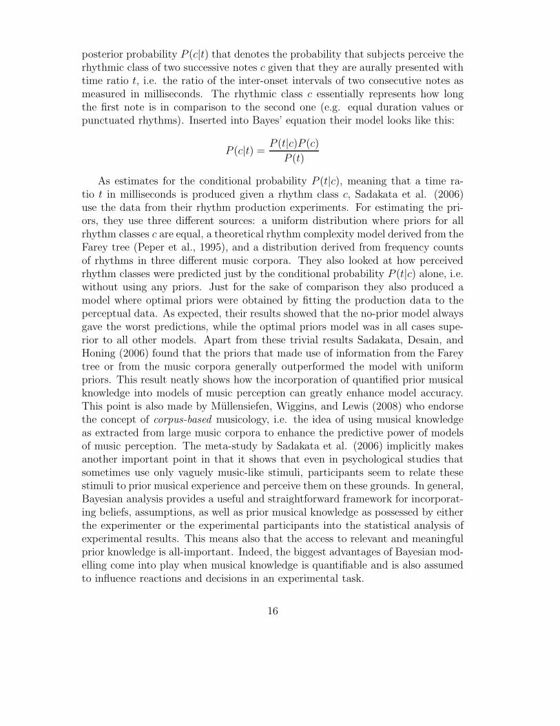
posterior probability P (c|t) that denotes the probability that subjects perceive therhythmic class of two successive notes c given that they are aurally presented withtime ratio t, i.e. the ratio of the inter-onset intervals of two consecutive notes asmeasured in milliseconds. The rhythmic class c essentially represents how longthe first note is in comparison to the second one (e.g. equal duration values orpunctuated rhythms). Inserted into Bayes’ equation their model looks like this:

P (c|t) =P (t|c)P (c)

P (t)

As estimates for the conditional probability P (t|c), meaning that a time ra-tio t in milliseconds is produced given a rhythm class c, Sadakata et al. (2006)use the data from their rhythm production experiments. For estimating the pri-ors, they use three different sources: a uniform distribution where priors for allrhythm classes c are equal, a theoretical rhythm complexity model derived from theFarey tree (Peper et al., 1995), and a distribution derived from frequency countsof rhythms in three different music corpora. They also looked at how perceivedrhythm classes were predicted just by the conditional probability P (t|c) alone, i.e.without using any priors. Just for the sake of comparison they also produced amodel where optimal priors were obtained by fitting the production data to theperceptual data. As expected, their results showed that the no-prior model alwaysgave the worst predictions, while the optimal priors model was in all cases supe-rior to all other models. Apart from these trivial results Sadakata, Desain, andHoning (2006) found that the priors that made use of information from the Fareytree or from the music corpora generally outperformed the model with uniformpriors. This result neatly shows how the incorporation of quantified prior musicalknowledge into models of music perception can greatly enhance model accuracy.This point is also made by Mullensiefen, Wiggins, and Lewis (2008) who endorsethe concept of corpus-based musicology, i.e. the idea of using musical knowledgeas extracted from large music corpora to enhance the predictive power of modelsof music perception. The meta-study by Sadakata et al. (2006) implicitly makesanother important point in that it shows that even in psychological studies thatsometimes use only vaguely music-like stimuli, participants seem to relate thesestimuli to prior musical experience and perceive them on these grounds. In general,Bayesian analysis provides a useful and straightforward framework for incorporat-ing beliefs, assumptions, as well as prior musical knowledge as possessed by eitherthe experimenter or the experimental participants into the statistical analysis ofexperimental results. This means also that the access to relevant and meaningfulprior knowledge is all-important. Indeed, the biggest advantages of Bayesian mod-elling come into play when musical knowledge is quantifiable and is also assumedto influence reactions and decisions in an experimental task.

16

3 Music Modelling

The distinction between research in cognitive music psychology and what we callmusic modelling is admittedly not very clear-cut and sometimes simply a matter ofperspective. While the studies reviewed in the last section are primarily interestedin mental processes connected to music perception and cognition by observinghuman behaviour that reflects these mental processes, the studies that we nowlook at rather try to describe the structure of music itself statistically. Of course,descriptions and representations of musical structure are always a result of humancognition, but studies of music modelling tend to be less interested in the natureof the underlying psychological processes that generate musical structures than inthe structures themselves.

Modelling music data has become increasingly popular in recent times, duelargely to the increasing amount of music that is digitally available in a symbolicencoding format (e.g. MIDI, EsAC, kern, or other codes that encode notes asthe basic musical events). While statistical approaches for describing the compo-sitional structure of music have been present since the 1950s (e.g. Meyer, 1957;Moles, 1958; Steinbeck, 1982; Fucks, 1962; Fucks & Lauter, 1965; Fucks, 1968), thenumber and diversity of statistical approaches for modelling structural features ofmusic have rocketed over the last decade.

3.1 Bayesian models of musical structure

Also for describing musical structures, Bayesian modelling has become quite pop-ular (e.g., Temperley, 2004, 2006, 2007; Rhodes et al., 2007). As an example, wetake Temperley’s description of a Bayesian model that determines the key of agiven piece or segment of music (Temperley, 2004). At its core we find Bayes’ rulethat calculates the probability of a musical feature or structure (here: the key)given an empirical music surface (here: the frequencies of pitch classes in a musicalsegment).

P (key structure | surface) ∝∏

segment

(

M∏

p

Kpc

∏

∼p

(1 − Kpc)

)

Here, M is a modulation score that penalises the change in key from one segmentto the next and Kpc stands for the key-profile values of the pitch-classes present(p) in a segment which are multiplied by the product of (1 − Kpc) for all pitch-classes not present in this segment (∼ p). Thus, the probability computation formusical keys, given the pitch classes of a musical piece, is based on the relativefrequency with which the twelve scale degrees appear in a key as well as on theprobability of a subsequent segment of the piece being in the same key as the

17

previous segment. Comparable to the testing of different priors as in the study bySadakata et al. (2006), Temperley uses pitch-class profiles derived from differentsources (music collections or corpora). Tested against other key finding modelslike his own non-Bayesian model (Temperley, 2001) or the Krumhansl-Schmuckleralgorithm (Krumhansl, 1990), his Bayesian model achieves about equal successrates, although, as Temperley openly admits, most of the core features of themodel may be formulated without Bayesian terminology and notation. Reviewinghis recent book (Pearce et al., 2007) on probabilistic models and music (Temperley,2007), it seems that Temperley has not yet made full use of the potential that theBayesian approach can offer for modelling musical structures. It appears thatBayesian modelling in this sense is largely concerned with precisely quantifyingrule-based systems of musical analysis. Therefore, it remains to be seen what theoriginal Bayesian contribution to these kinds of musical models will be, consideringthat frequency counts on musical elements have been successfully used as predictorsin non-Bayesian models before (e.g. Eerola et al., 2002; Costa et al., 2004).

3.2 n-gram models of musical structure

Another recent, prominent trend in music modelling is the use of Markov-chainsor n-gram modelling. Here, the basic musical units are longer sequence structures,instead of single events such as pitches, intervals, or durations. This approachbuilds on the basic assumption that music is principally produced and perceivedas a time-ordered set of events, be it tones of a melody or harmonies in a polyphonicpiece. The notion that music can be explained, taught, and analysed as formulaehas been around for several hundred years in music theory, but only due to therecent availability of large electronic corpora can these hypotheses be empiricallytested.

A sophisticated example of the n-gram approach is the work of Pearce andWiggins (e.g. 2004, 2006) which is concerned with melodic n-grams. Their re-search hypothesis is that many aspects of musical expectation are acquired throughspontaneous induction of sequential regularities in the music we are exposed to.Consequently, they name their model the Information Dynamics of Music model,or short the IDyoM model, and define it as a model of sequences ei composed ofsymbols drawn from an alphabet E . The model estimates the conditional proba-bility of an element at index i in the sequence, given the preceding elements in thesequence: p(ei|e

i−1

1). Given such a model, the degree to which an event appearing

in a melody is unexpected can be defined as the information content (MacKay,2003), h(ei|e

i−1

1), of the event, given the context:

h(ei|ei−1

1) = log

2

1

p(ei|ei−1

1).

18

The information content can be interpreted as the contextual unexpectedness orsurprise associated with the event. The contextual uncertainty of the model’sexpectations in a given melodic context can be defined as the entropy (or averageinformation content) of the predictive context itself:

H(ei−1

1) =

∑

ei∈E

p(ei|ei−1

1)h(ei|e

i−1

1).

Just as in the Bayesian model reviewed above, this model builds on counts ofoccurrences of melodic n-grams in a collection of melodies. For a given melodiccontext, the model returns the continuation of chain of n-1 notes with maximumlikelihood as a prediction for the given context. Although the idea of recordingthe frequencies of melodic n-grams in a corpus and returning the like for any givencontext sounds quite straight forward, the details of their modelling are quiteintricate and consist of techniques adopted from statistical language learning anddata compression, which are outside the scope of what can be explained herein detail. Pearce and Wiggins (2004) examine several model parameters, first,the model type, where they find best results by employing a combination of along-term model trained on large corpora of melodies (e.g. the Essen folk songcollection, church hymns, ballads), and a short-term model trained exclusivelyon the melody currently being predicted. Second, they place emphasis on thetreatment of novel n-grams when encountered in a prediction context for whichno frequency count yet exists in the model. Here, smoothing and escape heuristicsare explored from automatic speech processing. As a third and important modelparameter, they vary the upper order bound (maximal length) of the n-gramsconsidered. In combination with other parameters a variant yields optimal modelperformance where the order of the n-gram is unbound but the relative weightof a n-gram is adjusted according to its length, for the averaged prediction givesmore weight to longer n-grams. A fourth and decisive set of model parameters isthe type of abstraction or transformation to be applied to the raw melody data,where they determine a handful of musically meaningful view points (i.e. musicaldimensions or parameters such as raw pitches, pitch intervals, note durations)through a standard variable selection process (step-wise variable elimination).

As a result from this search through the parameter space, Pearce and Wiggins(2006) are able to predict experimental data from three previous studies (Cuddy &Lunney, 1995; ?, ?, ?) where expectation of melodic continuation was determinedfrom behavioural experiments with human listeners. Their model performs wellon all three data sets and outperforms a competing model proposed by Narmour(1990) based on principles of Gestalt psychology (implemented by Schellenberg,1997). Pearce and Wiggins’ reasoning (2006) regarding model selection is a notablepoint of their approach and can serve as a guideline for other studies concerned with

19

the comparison of models for music cognition. As a criterion for model selection,they do not only consider data fit, but also scope (which is the model’s failure topredict random data), and simplicity (which is the number of prior assumptionsand principles the model builds upon).

Strong evidence in favour of the IDyoM model as a general model of melodyperception comes from a number of recent studies where the model was not usedfor its original purpose (i.e. to predict melodic expectation), but was applied toautomatically segment full melodies into melodic phrases. The underlying ratio-nale is that perceptual groups are associated with points of closure where theongoing cognitive process of expectation is disrupted either because the melodiccontext fails to stimulate strong expectations for any particular continuation orbecause the actual continuation is unexpected. For predicting the manual phrasesegmentations of 1705 folk songs from the Essen collection which were annotatedby expert folk song collectors, the IDyoM model performed at a comparable levelof accuracy to a couple of other computational models. The surprising result of thisstudy was the fact that IDyoM as a model of melodic expectation did almost aswell as existing models that were specifically designed for segmenting melodies (e.g.Grouper, Temperley, 2001, and LBDM, Cambouropoulos, 2001) and make use ofhigh-level music theoretical knowledge about melody segmentation (see Pearce etal., 2008). The fact that the model generates acceptable results outside its origi-nal application domain let the authors hypothesise that mechanisms of statisticallearning which are the core of the IDyoM model, actually represent the underlyingprocesses of melody perception as well as the acquisition of musical knowledge.

4 Conclusion

This update intends to highlight some of the more interesting statistical approachesas employed in recent music psychology research and aims at motivating music psy-chologists to explore the analytical and epistemological possibilities that these newtechniques provide. Naturally, a short overview like this can only be far from com-plete, both in terms of depth (of the mathematical technicalities and the designof studies reviewed) as well as in terms of the range of new techniques covered.Nonetheless, we hope that this paper serves as an overview of current trends sothat music psychologists might obtain an idea of where empirical methodologyis heading. Some final remarks have to be made on the available software thatallows to compute analyses using the methods described. Only if software is avail-able and accessible as well as easy to handle, new statistical techniques have achance of becoming a popular research tool and will possibly be integrated intothe canon of methods. While in the past, music psychologists were often depen-dent on a few specialised companies to integrate a new technique into commercial

20

software packages such as SPSS, SAS, or Statistica with graphical user interfaces(GUIs), the success of powerful and yet high-level programming languages thatare specially designed for data analysis or, at least, have large libraries designedfor scientific statistical computing, opens a new range of possibilities. The mostimportant of these very high-level data analysis environments are Weka3 (whichincludes a GUI), Matlab4 (Statistics Toolbox ), R5, S-Plus6, and Python7(SciPyand StatPy packages). Researchers and software developers around the globe con-stantly contribute codes for new statistical analysis to these environments thatare then available to music psychologists who, in general, are not keen to imple-ment new statistical procedures from scratch themselves. Apart from Matlab andS-Plus, which require an expensive license for the basic system and commercialtoolboxes, the usage of the other aforementioned data analysis environments isfree.

Regarding the statistical techniques covered in this paper, general multidimen-sional scaling packages, including INDSCAL, are implemented in most commer-cial as well as free software programmes. Unfortunately, the discussed CLASCALmodel is not yet available in any larger environment. In contrast, classification andregression trees (often called decision trees) have implementations in most environ-ments. The studies cited above made use of the R-package CART. Functional dataanalysis packages are maintained for Matlab, R, and S-Plus. For basic reasoningwith Bayes’ theorem, no special software is required. But there is a wealth of ad-vanced Bayesian methods available that we did not cover here, since for almost allsoftware environments more or less comprehensive Bayesian packages or librariesare obtainable. Finally, the IDyoM model is unfortunately not publicly available.But many programmes provide the basic tools for sequence-based methods oftenemployed in computational linguistics (e.g. package tm in R, Clementine in SPSSor KEA in Weka).

Acknowledgements

Daniel Mullensiefen is supported by EPSRC grant EP/D038855/1. We would liketo thank Alex McLean and Klaus Frieler for valuable comments on earlier versionsof the manuscript.

3http://www.cs.waikato.ac.nz/ml/weka/4http://www.mathworks.com/5http://www.r-project.org/6http://www.insightful.com/7http://www.python.org/

21

References

Almansa, J., & Delicado, P. (2009 (in press)). Analysing musical perfor-mance through functional data analysis: Rhythmic structure in schumann’straumerei. Connection Science.

Beran, J. (2004). Statistics in musicology. Boca Raton: Chapman Hall.Bharucha, J. J. (1987). Music cognition and perceptual facilitation: A connec-

tionist framework. Music Perception, 5, 1-30.Bharucha, J. J., & Krumhansl, C. L. (1983). The representation of harmonic struc-

ture in music: Hierarchies of stability as a function of context. Cognition,13, 63-102.

Bottcher, H. F., & Kerner, U. (1978). Methoden in der musikpsychologie. Leipzig:C. F. Peters.

Breiman, L., Friedman, J., Olshen, R., & Stone, C. (1984). Classification andregression trees. Belmont (CA): Wadsworth.

Burgoyne, J., & McAdams, S. (2007). Non-linear scaling techniques for uncoveringthe perceptual dimensions of timbre. In In proceedings of the internationalcomputer music conference (icmc 2007) (Vol. 1, p. 73-76).

Caclin, A., McAdams, S., Smith, B., & Winsberg, S. (2005). Acoustic correlatesof timbre space dimensions: A confirmatory study using synthetic tones.Journal of the Acoustical Society of America, 118 (1), 471-482.

Cambouropoulos, E. (2001). The local boundary detection model (lbdm) and itsapplication in the studt of expressive timing. In Proceedings of the interna-tional computer music conference (p. 17-22). San Francisco: ICMA.

Carroll, J., & Chang, J. (1970, 283-319). Analysis of individual difference sinmultidimensional scaling via an n-way generalization of eckart-young decom-position. Psychometrika, 52, 35.

Chater, N., & Manning, C. (2006). Probabilistic models of language processingand acquisition. TRENDS in Cognitive Sciences, 10 (7), 335-344.

Chater, N., & Oaksford, M. (2007). Bayesian rationality. the probabilistic approachto human reasoning. Oxford: Oxford University Press.

Chater, N., Tenenbaum, J., & Yuille, A. (2006). Probabilistic models of cognition:conceptual foundations. TRENDS in Cognitive Sciences, 10 (7), 287-291.

Costa, M., Fine, P., & Ricci Bitti, P. E. (2004, September). Interval distribution,mode, and tonal strength of melodies as predictors of perceived emotion.Music Perception, 22 (1), 1-14.

Cuddy, L. L., & Lunney, C. (1995). Expectancies generated by melodic intervals:Perceptual judgments of melodic continuity. Perception & Psychophysics,57, 451-462.

Desain, P., & Honing, H. (1992). Music, mind and machine, studies in com-

22

puter music, music cognition and artificial intelligence. Amsterdam: ThesisPublishers.

Eerola, T., Jarvinen, T., Louhivuori, J., & Toiviainen, P. (2002, March). Statisticalfeatures and perceived similarity of folk melodies. Music Perception, 18 (3),275-296.

Flexer, A. (2006). Statistical evaluation of music information retrieval experiments.Journal of New Music Research, 35 (2), 113-120.

Fucks, W. (1962). Mathematical analysis of formal structure of music. IEEETransactions Information Theory, 8 (5), 225-228.

Fucks, W. (1968). Nach allen regeln der kunst. Stuttgart: DVA.Fucks, W., & Lauter, J. (1965). Exaktwissenschaftliche musikanalyse. Opladen:

Westdeutscher Verlag.Gromko, J. E. (1993). Perceptual differences between expert and novice music

listeners at multidimensional scaling analysis. Psychology of Music, 21, 34-47.

Kendall, R. A., & Carterette, E. (1991). Perceptual scaling of simultaneous windinstrument timbres. Music Perception, 8, 360-404.

Kopiez, R., Weihs, C., Ligges, U., & Lee, J. I. (2006, October). Classification ofhigh and low achievers in a music sight-reading task. Psychology of Music,34 (1), 5-26.

Krimphoff, J., McAdams, S., & Winsberg, S. (1994). Caracterisation du timbredes sons complexes. ii: Analyses acoustique et quantification psychophysique.Journal de Physique, 4 (C5), 625-628.

Krumhansl, C. L. (1990). Cognitive foundations of musical pitch. Oxford: OxfordUniversity Press.

Krumhansl, C. L., & Kessler, E. (1982). Tracing the dynamic changes in perceivedtonal organization in a spatial representation of musical keys. PsychologicalReview, 89, 334-368.

Levitin, D. J., Nuzzo, R. L., Vines, B. W., & Ramsay, J. O. (2007). Introductionto functional data analysis. Canadian Psychology, 48 (3), 135-155.

Lippens, S., Martens, J.-P., De Mulder, T., & Tzanetakis, G. (2004). A comparisonof human and automatic musical genre classification. In Ieee internationalconference on acoustics, speech, and signal processing (icassp) (Vol. 4, p.223-236).

MacKay, D. (2003). Information theory, inference, and learning algorithms. Cam-bridge: Cambridge University Press.

Markuse, B., & Schneider, A. (1996). Ahnlichkeit, nahe, distanz: zur anwendungmultidimensionaler skalierung in musik-wissenschaftlichen untersuchun-gen. Systematische Musikwissenschaft/ Systematic Musicology/Musicologiesystematique, 4, 53-89.

23

McAdams, S., Winsberg, S., Donnadieu, S., De Soete, G., & Krimphoff, J. (1995).Perceptual sclaing of synthesized musical timbres: ommon dimensions, speci-ficities, and latent subject classes. Psychological Research, 58, 177-192.

Meyer, L. B. (1957). Meaning in music and information theory. Journal ofAesthetics and Art Criticism, 15, 412-424.

Moles, A. (1958). Theorie de l’information et perception estetique. Paris: Flam-marion.

Mullensiefen, D. (2004). Variabilitat und konstanz von melodien in der erinnerung.ein beitrag zur musikpsychologischen gedachtnisforschung. [variability andconstancy of remembered melodies: A music-psychological investigation ofmemory]. Unpublished doctoral dissertation, University of Hamburg.

Mullensiefen, D., & Hennig, C. (2006). Modeling memory for melodies. In M. Sil-iopoulou, R. Kruse, C. Borgelt, A. Nurnberger, & W. Gaul (Eds.), Fromdata and information analysis to knowledge engineering (p. 732-739). Berlin:Springer.

Mullensiefen, D., Wiggins, G., & Lewis, D. (2008). High-level feature descriptorsand corpus-based musicology: Techniques for modelling music cognition. InA. Schneider (Ed.), Systematic and comparative musicology: Concepts, meth-ods, findings (Vol. 24, p. 133-155). Frankfurt: Peter Lang.

Narmour, E. (1990). he analysis and cognition of basic melodic structures: Theimplication-realization model. Chicago: University of Chicago Press.

Orio, N. (2006, November). Music retrieval: A tutorial and review. Foundationsand Trends in Information Retrieval, 1 (1), 1-90.

Pearce, M. T., Mullensiefen, D., Rhodes, C., & Lewis, D. (2007). David temperley,music and probability (review). Empirical Musicology, 2 (4), 155-163.

Pearce, M. T., Mullensiefen, D., & Wiggins, G. A. (2008). A comparison ofstatistical and rule-based models of melodic segmentation. In Proceedings ofthe 9th international conference on music information retrieval.

Pearce, M. T., & Wiggins, G. A. (2004). Improved methods for statistical mod-elling of monophonic music. Journal of New Music Research, 33 (4), 367-385.

Pearce, M. T., & Wiggins, G. A. (2006, June). Expectation in melody: Theinfluence of context and learning. Music Perception, 23 (5), 377-405.

Peper, C., Beek, P., & Wieringen, P. van. (1995). Multifrequency coordinationin bimanual tapping: Asymmetrical coupling and signs of supercriticality.Journal of Experimental Psychology: Human Perception and Performance,21, 117-1138.

Ramsay, J. O., & Silverman, B. W. (2005). Functional data analysis. Berlin:Springer.

Repp, B. H. (1992). Diversity and commonality in music performance: An analysisof timing microstructure in schumann’s traumerei. Journal of the Acoustical

24

Society of America, 92 (5), 2546-2568.Rhodes, C., Lewis, D., & Mullensiefen, D. (2007). Bayesian model selection

for harmonic labelling. In Program and summaries of the first internatinalconfernece of the society for mathematics and computation in music, berlin,may, 18-20, 2007.

Sadakata, M., Desain, P., & Honing, H. (2006, February). The bayesian way torelate rhythm perception and production. Music Perception, 23 (3), 269-288.

Sahmer, K., Vigneau, E., & Qannari, E. (2006). A cluster approach to analyzepreference data: Choice of the number of clusters. Food Quality and Prefer-ence, 17 (3-4), 257-265.

Schellenberg, E. G. (1997). Simplifying the implication-realization model of sim-plifying the implication-realization model of melodic expectancy. Music Per-ception, 14, 295-318.

Schubert, E., & Dunsmuir, W. (1999). Regression modelling continuous data inmusic psychology. In S. W. Yi (Ed.), Music, mind, and science (p. 298-352).Seoul: National University Press.

Schumaker, L. (1981). Spline functions: Basic theory. John Wiley and Sons.Steinbeck, W. (1982). Struktur und ahnlichkeit: Methoden automatisierter

melodieanalyse. Kassel: Barenreiter.Temperley, D. (2001). The cognition of basic musical structures. Cambridge, MA:

MIT Press.Temperley, D. (2004, Fall). Bayesian models of musical structure and cognition.

Musicae Scientiae, 8 (2), 175-205.Temperley, D. (2006). A probabilistic model of melody perception. In Proceeding

of the 7th international conference on music information retrieval.Temperley, D. (2007). Music and probability. Cambridge, MA: MIT Press.Therneau, T., & Atkinson, E. (1997). An introduction to recursive partitioning

using the rpart routines (Tech. Rep.). Mayo Clinic Division of Biostatistics.Tillmann, B., Bharucha, J. J., & Bigand, E. (2003). Learning and perceiving

musical structures: further insights from artificial neural networks. In R. Za-torre & I. Peretz (Eds.), The cognitive neuroscience of music (p. 109-123).Oxford: Oxford University Press.

Vines, B. W., Krumhansl, C. L., Wanderley, M. M., & Levitin, D. J. (2006). Cross-modal interactions in the perception of musical performance. Cognition, 101,80-113.

Vines, B. W., Nuzzo, R. L., & Levitin, D. J. (2005, December). Analyzing tem-poral dynamics in music: Differential calculus, physics, and functional dataanalysis techniques. Music Perception, 23 (2), 137-152.

Windsor, L. (2001). Data collection, experimental design, and statistics in musi-cal research. In E. Clarke & N. Cook (Eds.), Empirical musicology: Aims,

25

methods, prospects (p. 197-222). Oxford: Oxford University Press.Winsberg, S., & De Soete, G. (1993). A latent class approach to fitting the

weighted euclidean model, clascal. Psychometrika, 58, 315-330.Wundt, W. (1882). Uber musikpsychologische methoden. In Philosophische

schriften (Vol. 1, p. 138).

26