Statistical Tables - Department of Zoology, UBCbio300/StatTables.pdf · Statistical Tables from...

Statistical Tables from Whitlock & Schluter – The Analysis of Biological Data© Whitlock & Schluter, all rights reserved- Do not distribute without consent of the authors

Statistical Tables

This appendix gives numerical values for a few of the most commonly used probability

distributions. More can be found in references such as Rohlf and Sokal, Biostatistical

Tables.

Statistical Table A: χ2 distributions

Statistical Table B: Z distribution

Statistical Table C: Student's t distribution

Statistical Table D: F distribution

Statistical Table E: Mann-Whitney U distribution

Statistical Table F: The correlation coefficient, r.

Statistical Table G: Tukey-Kramer critical values

Statistical Table H: Critical Values for the Spearman's correlation

Statistical Tables 2

© Whitlock & Schluter, all rights reserved- Do not distribute without consent of the authors

Using statistical tables

With easy access to computers becoming more common, statistical tables become less

and less necessary. It is much better to give a precise P-value calculated by computer

than to say simply P < 0.05, etc. For at least the basic distributions, such as the standard

normal, χ2 , Student's t, F, etc., computer programs such as an y statistical program,

Excel, Mathematica, etc, can calculate exact P-values easily. Statistical tables can be

used when computers are unavailable, or when only an approximate answer is

satisfactory.

Statistical tables can only give a limited amount of information, limited as they are by

space. The tables that follow usually only give critical value s that correspond to a few

values of α.. Moreover, not all values of the degrees of freedom are shown. If an analysis

requires a critical value for a test statistic with a number of degrees of freedom not shown

in the table, then there are several methods available to approximate the critical value

from the information that is available in the table. If there the number of degrees of

freedom desired is between two values addressed by the table, then there are two options,

in order of difficulty.

(1) The conservative approach: Find the two values of the degrees of freedom that are

given in the table and are closest to the desired value, above and below the desired value.

Choose the one that makes it most difficult to reject the null hypothesis. Use this value.

(2) Extrapolation: Find the critical values that correspond to the degrees of freedom

given in the table just above and just below the desired df. Call the df values given in the

Statistical Tables 3


table bracketing the desired degrees of freedom dflow and dfhigh, and the critical values

corresponding to each CVlow and CVhigh. Imagine drawing a line from the point given by

the dflow and CVlow to the point given by dfhigh and CVhigh. Move along this line

proportionally as far as the distance from dflow to the desired df. The critical value at that

point along the line is the extrapolated critical value. By equation, this gives the

extrapolated critical value.

€

CV = CVlow + CVhigh −CVlow( ) df − dflowdfhigh − dflow

For example, Statistical Table D gives critical values for the F distribution. Imagine that

we needed the critical value of F with 1 and 120 degrees of freedom in the numerator and

denominator, respectively, for a one-tailed test with α = 0.05. The table gives a column

for df = 1 in the numerator, but skips from df = 100 to df = 200 for the denominator. We

therefore look up the value for the closest number of denominator df less than 120 (df =

100) and the value for the closest df above 120 (df= 200). These are

€

F0.05(1),1,100 = 3.94 and

€

F0.05(1),1,200 = 3.89 . We can use extrapolation to find the critical value for

€

F0.05(1),1,120 :

€

CV = CVlow + CVhigh −CVlow( ) df − dflowdfhigh − dflow

= 3.94 + 3.89 − 3.94( ) 120 −100200 −100

= 3.93

In other words, 120 is 20% from 100 to 120, so we find that the desired critical value

3.93 is 20% of the way from 3.94 to 3.89.


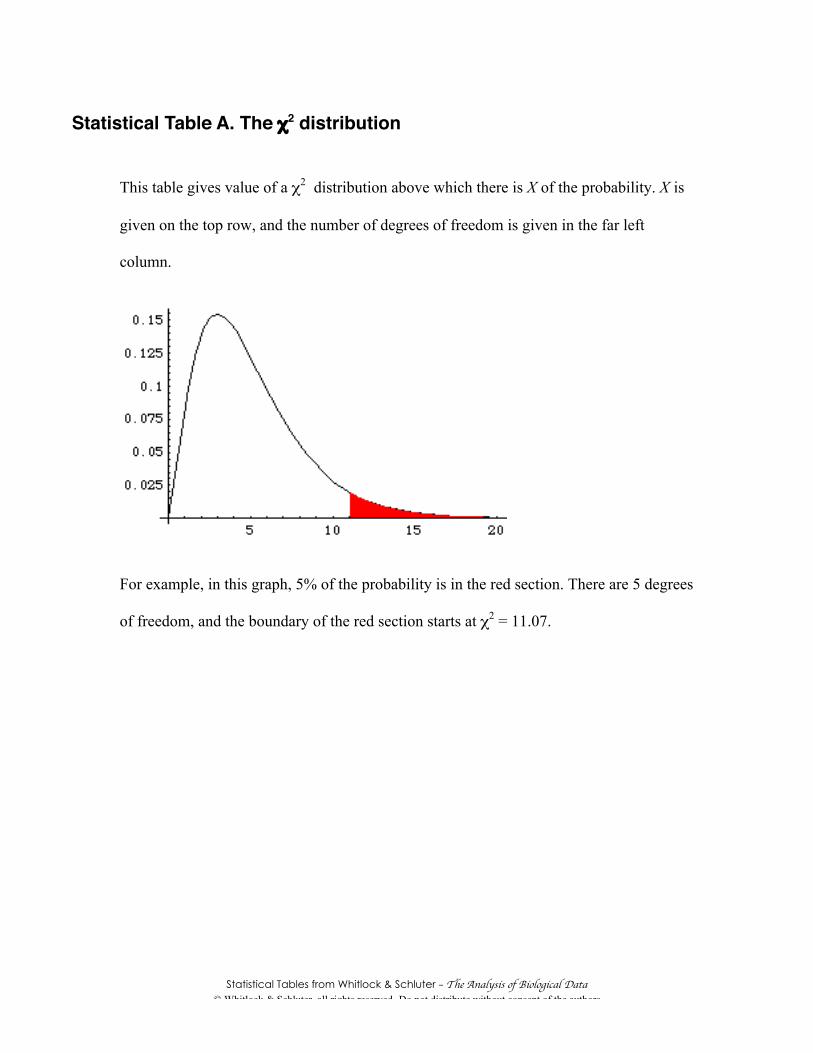
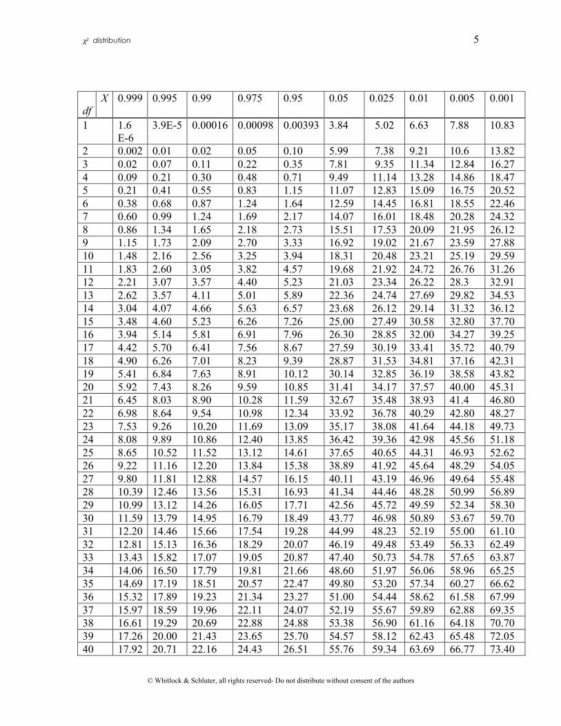
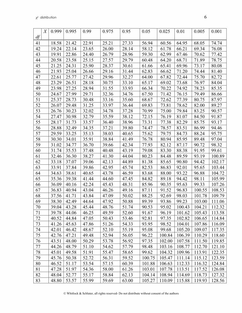
Statistical Table A. The χ2 distribution

This table gives value of a χ2 distribution above which there is X of the probability. X is

given on the top row, and the number of degrees of freedom is given in the far left

column.

For example, in this graph, 5% of the probability is in the red section. There are 5 degrees

of freedom, and the boundary of the red section starts at χ2 = 11.07.

χ2 distribution 5


0.999 0.995 0.99 0.975 0.95 0.05 0.025 0.01 0.005 0.001df

X

1 1.6E-6

3.9E-5 0.00016 0.00098 0.00393 3.84 5.02 6.63 7.88 10.83

2 0.002 0.01 0.02 0.05 0.10 5.99 7.38 9.21 10.6 13.823 0.02 0.07 0.11 0.22 0.35 7.81 9.35 11.34 12.84 16.274 0.09 0.21 0.30 0.48 0.71 9.49 11.14 13.28 14.86 18.475 0.21 0.41 0.55 0.83 1.15 11.07 12.83 15.09 16.75 20.526 0.38 0.68 0.87 1.24 1.64 12.59 14.45 16.81 18.55 22.467 0.60 0.99 1.24 1.69 2.17 14.07 16.01 18.48 20.28 24.328 0.86 1.34 1.65 2.18 2.73 15.51 17.53 20.09 21.95 26.129 1.15 1.73 2.09 2.70 3.33 16.92 19.02 21.67 23.59 27.8810 1.48 2.16 2.56 3.25 3.94 18.31 20.48 23.21 25.19 29.5911 1.83 2.60 3.05 3.82 4.57 19.68 21.92 24.72 26.76 31.2612 2.21 3.07 3.57 4.40 5.23 21.03 23.34 26.22 28.3 32.9113 2.62 3.57 4.11 5.01 5.89 22.36 24.74 27.69 29.82 34.5314 3.04 4.07 4.66 5.63 6.57 23.68 26.12 29.14 31.32 36.1215 3.48 4.60 5.23 6.26 7.26 25.00 27.49 30.58 32.80 37.7016 3.94 5.14 5.81 6.91 7.96 26.30 28.85 32.00 34.27 39.2517 4.42 5.70 6.41 7.56 8.67 27.59 30.19 33.41 35.72 40.7918 4.90 6.26 7.01 8.23 9.39 28.87 31.53 34.81 37.16 42.3119 5.41 6.84 7.63 8.91 10.12 30.14 32.85 36.19 38.58 43.8220 5.92 7.43 8.26 9.59 10.85 31.41 34.17 37.57 40.00 45.3121 6.45 8.03 8.90 10.28 11.59 32.67 35.48 38.93 41.4 46.8022 6.98 8.64 9.54 10.98 12.34 33.92 36.78 40.29 42.80 48.2723 7.53 9.26 10.20 11.69 13.09 35.17 38.08 41.64 44.18 49.7324 8.08 9.89 10.86 12.40 13.85 36.42 39.36 42.98 45.56 51.1825 8.65 10.52 11.52 13.12 14.61 37.65 40.65 44.31 46.93 52.6226 9.22 11.16 12.20 13.84 15.38 38.89 41.92 45.64 48.29 54.0527 9.80 11.81 12.88 14.57 16.15 40.11 43.19 46.96 49.64 55.4828 10.39 12.46 13.56 15.31 16.93 41.34 44.46 48.28 50.99 56.8929 10.99 13.12 14.26 16.05 17.71 42.56 45.72 49.59 52.34 58.3030 11.59 13.79 14.95 16.79 18.49 43.77 46.98 50.89 53.67 59.7031 12.20 14.46 15.66 17.54 19.28 44.99 48.23 52.19 55.00 61.1032 12.81 15.13 16.36 18.29 20.07 46.19 49.48 53.49 56.33 62.4933 13.43 15.82 17.07 19.05 20.87 47.40 50.73 54.78 57.65 63.8734 14.06 16.50 17.79 19.81 21.66 48.60 51.97 56.06 58.96 65.2535 14.69 17.19 18.51 20.57 22.47 49.80 53.20 57.34 60.27 66.6236 15.32 17.89 19.23 21.34 23.27 51.00 54.44 58.62 61.58 67.9937 15.97 18.59 19.96 22.11 24.07 52.19 55.67 59.89 62.88 69.3538 16.61 19.29 20.69 22.88 24.88 53.38 56.90 61.16 64.18 70.7039 17.26 20.00 21.43 23.65 25.70 54.57 58.12 62.43 65.48 72.0540 17.92 20.71 22.16 24.43 26.51 55.76 59.34 63.69 66.77 73.40

χ2 distribution 6


0.999 0.995 0.99 0.975 0.95 0.05 0.025 0.01 0.005 0.001df

X

41 18.58 21.42 22.91 25.21 27.33 56.94 60.56 64.95 68.05 74.7442 19.24 22.14 23.65 26.00 28.14 58.12 61.78 66.21 69.34 76.0843 19.91 22.86 24.40 26.79 28.96 59.30 62.99 67.46 70.62 77.4244 20.58 23.58 25.15 27.57 29.79 60.48 64.20 68.71 71.89 78.7545 21.25 24.31 25.90 28.37 30.61 61.66 65.41 69.96 73.17 80.0846 21.93 25.04 26.66 29.16 31.44 62.83 66.62 71.20 74.44 81.4047 22.61 25.77 27.42 29.96 32.27 64.00 67.82 72.44 75.70 82.7248 23.29 26.51 28.18 30.75 33.10 65.17 69.02 73.68 76.97 84.0449 23.98 27.25 28.94 31.55 33.93 66.34 70.22 74.92 78.23 85.3550 24.67 27.99 29.71 32.36 34.76 67.50 71.42 76.15 79.49 86.6651 25.37 28.73 30.48 33.16 35.60 68.67 72.62 77.39 80.75 87.9752 26.07 29.48 31.25 33.97 36.44 69.83 73.81 78.62 82.00 89.2753 26.76 30.23 32.02 34.78 37.28 70.99 75.00 79.84 83.25 90.5754 27.47 30.98 32.79 35.59 38.12 72.15 76.19 81.07 84.50 91.8755 28.17 31.73 33.57 36.40 38.96 73.31 77.38 82.29 85.75 93.1756 28.88 32.49 34.35 37.21 39.80 74.47 78.57 83.51 86.99 94.4657 29.59 33.25 35.13 38.03 40.65 75.62 79.75 84.73 88.24 95.7558 30.30 34.01 35.91 38.84 41.49 76.78 80.94 85.95 89.48 97.0459 31.02 34.77 36.70 39.66 42.34 77.93 82.12 87.17 90.72 98.3260 31.74 35.53 37.48 40.48 43.19 79.08 83.30 88.38 91.95 99.6161 32.46 36.30 38.27 41.30 44.04 80.23 84.48 89.59 93.19 100.8962 33.18 37.07 39.06 42.13 44.89 81.38 85.65 90.80 94.42 102.1763 33.91 37.84 39.86 42.95 45.74 82.53 86.83 92.01 95.65 103.4464 34.63 38.61 40.65 43.78 46.59 83.68 88.00 93.22 96.88 104.7265 35.36 39.38 41.44 44.60 47.45 84.82 89.18 94.42 98.11 105.9966 36.09 40.16 42.24 45.43 48.31 85.96 90.35 95.63 99.33 107.2667 36.83 40.94 43.04 46.26 49.16 87.11 91.52 96.83 100.55 108.5368 37.56 41.71 43.84 47.09 50.02 88.25 92.69 98.03 101.78 109.7969 38.30 42.49 44.64 47.92 50.88 89.39 93.86 99.23 103.00 111.0670 39.04 43.28 45.44 48.76 51.74 90.53 95.02 100.43 104.21 112.3271 39.78 44.06 46.25 49.59 52.60 91.67 96.19 101.62 105.43 113.5872 40.52 44.84 47.05 50.43 53.46 92.81 97.35 102.82 106.65 114.8473 41.26 45.63 47.86 51.26 54.33 93.95 98.52 104.01 107.86 116.0974 42.01 46.42 48.67 52.10 55.19 95.08 99.68 105.20 109.07 117.3575 42.76 47.21 49.48 52.94 56.05 96.22 100.84 106.39 110.29 118.6076 43.51 48.00 50.29 53.78 56.92 97.35 102.00 107.58 111.50 119.8577 44.26 48.79 51.10 54.62 57.79 98.48 103.16 108.77 112.70 121.1078 45.01 49.58 51.91 55.47 58.65 99.62 104.32 109.96 113.91 122.3579 45.76 50.38 52.72 56.31 59.52 100.75 105.47 111.14 115.12 123.5980 46.52 51.17 53.54 57.15 60.39 101.88 106.63 112.33 116.32 124.8481 47.28 51.97 54.36 58.00 61.26 103.01 107.78 113.51 117.52 126.0882 48.04 52.77 55.17 58.84 62.13 104.14 108.94 114.69 118.73 127.3283 48.80 53.57 55.99 59.69 63.00 105.27 110.09 115.88 119.93 128.56

χ2 distribution 7


0.999 0.995 0.99 0.975 0.95 0.05 0.025 0.01 0.005 0.001df

X

84 49.56 54.37 56.81 60.54 63.88 106.39 111.24 117.06 121.13 129.8085 50.32 55.17 57.63 61.39 64.75 107.52 112.39 118.24 122.32 131.0486 51.08 55.97 58.46 62.24 65.62 108.65 113.54 119.41 123.52 132.2887 51.85 56.78 59.28 63.09 66.50 109.77 114.69 120.59 124.72 133.5188 52.62 57.58 60.10 63.94 67.37 110.90 115.84 121.77 125.91 134.7589 53.39 58.39 60.93 64.79 68.25 112.02 116.99 122.94 127.11 135.9890 54.16 59.20 61.75 65.65 69.13 113.15 118.14 124.12 128.30 137.2191 54.93 60.00 62.58 66.50 70.00 114.27 119.28 125.29 129.49 138.4492 55.70 60.81 63.41 67.36 70.88 115.39 120.43 126.46 130.68 139.6793 56.47 61.63 64.24 68.21 71.76 116.51 121.57 127.63 131.87 140.8994 57.25 62.44 65.07 69.07 72.64 117.63 122.72 128.80 133.06 142.1295 58.02 63.25 65.90 69.92 73.52 118.75 123.86 129.97 134.25 143.3496 58.80 64.06 66.73 70.78 74.40 119.87 125.00 131.14 135.43 144.5797 59.58 64.88 67.56 71.64 75.28 120.99 126.14 132.31 136.62 145.7998 60.36 65.69 68.40 72.50 76.16 122.11 127.28 133.48 137.80 147.0199 61.14 66.51 69.23 73.36 77.05 123.23 128.42 134.64 138.99 148.23100 61.92 67.33 70.06 74.22 77.93 124.34 129.56 135.81 140.17 149.45


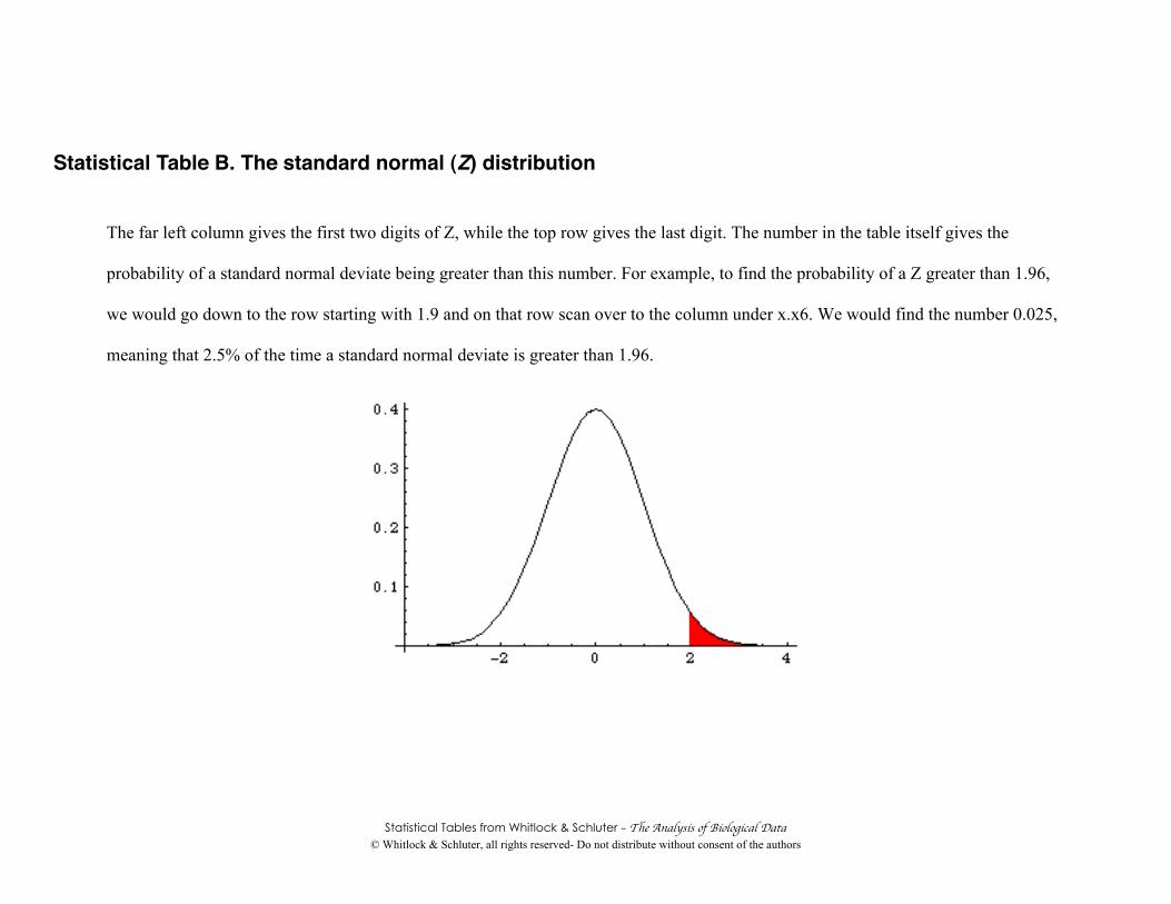
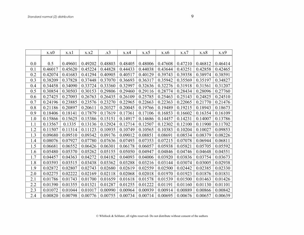
Statistical Table B. The standard normal (Z) distribution

The far left column gives the first two digits of Z, while the top row gives the last digit. The number in the table itself gives the

probability of a standard normal deviate being greater than this number. For example, to find the probability of a Z greater than 1.96,

we would go down to the row starting with 1.9 and on that row scan over to the column under x.x6. We would find the number 0.025,

meaning that 2.5% of the time a standard normal deviate is greater than 1.96.

Standard normal (Z) distribution 9


x.x0 x.x1 x.x2 .x3 x.x4 x.x5 x.x6 x.x7 x.x8 x.x9

0.0 0.5 0.49601 0.49202 0.48803 0.48405 0.48006 0.47608 0.47210 0.46812 0.464140.1 0.46017 0.45620 0.45224 0.44828 0.44433 0.44038 0.43644 0.43251 0.42858 0.424650.2 0.42074 0.41683 0.41294 0.40905 0.40517 0.40129 0.39743 0.39358 0.38974 0.385910.3 0.38209 0.37828 0.37448 0.37070 0.36693 0.36317 0.35942 0.35569 0.35197 0.348270.4 0.34458 0.34090 0.33724 0.33360 0.32997 0.32636 0.32276 0.31918 0.31561 0.312070.5 0.30854 0.30503 0.30153 0.29806 0.29460 0.29116 0.28774 0.28434 0.28096 0.277600.6 0.27425 0.27093 0.26763 0.26435 0.26109 0.25785 0.25463 0.25143 0.24825 0.245100.7 0.24196 0.23885 0.23576 0.23270 0.22965 0.22663 0.22363 0.22065 0.21770 0.214760.8 0.21186 0.20897 0.20611 0.20327 0.20045 0.19766 0.19489 0.19215 0.18943 0.186730.9 0.18406 0.18141 0.17879 0.17619 0.17361 0.17106 0.16853 0.16602 0.16354 0.161091.0 0.15866 0.15625 0.15386 0.15151 0.14917 0.14686 0.14457 0.14231 0.14007 0.137861.1 0.13567 0.1335 0.13136 0.12924 0.12714 0.12507 0.12302 0.12100 0.11900 0.117021.2 0.11507 0.11314 0.11123 0.10935 0.10749 0.10565 0.10383 0.10204 0.10027 0.098531.3 0.09680 0.09510 0.09342 0.09176 0.09012 0.08851 0.08691 0.08534 0.08379 0.082261.4 0.08076 0.07927 0.07780 0.07636 0.07493 0.07353 0.07215 0.07078 0.06944 0.068111.5 0.06681 0.06552 0.06426 0.06301 0.06178 0.06057 0.05938 0.05821 0.05705 0.055921.6 0.05480 0.05370 0.05262 0.05155 0.05050 0.04947 0.04846 0.04746 0.04648 0.045511.7 0.04457 0.04363 0.04272 0.04182 0.04093 0.04006 0.03920 0.03836 0.03754 0.036731.8 0.03593 0.03515 0.03438 0.03362 0.03288 0.03216 0.03144 0.03074 0.03005 0.029381.9 0.02872 0.02807 0.02743 0.02680 0.02619 0.02559 0.02500 0.02442 0.02385 0.023302.0 0.02275 0.02222 0.02169 0.02118 0.02068 0.02018 0.01970 0.01923 0.01876 0.018312.1 0.01786 0.01743 0.01700 0.01659 0.01618 0.01578 0.01539 0.01500 0.01463 0.014262.2 0.01390 0.01355 0.01321 0.01287 0.01255 0.01222 0.01191 0.01160 0.01130 0.011012.3 0.01072 0.01044 0.01017 0.00990 0.00964 0.00939 0.00914 0.00889 0.00866 0.008422.4 0.00820 0.00798 0.00776 0.00755 0.00734 0.00714 0.00695 0.00676 0.00657 0.00639

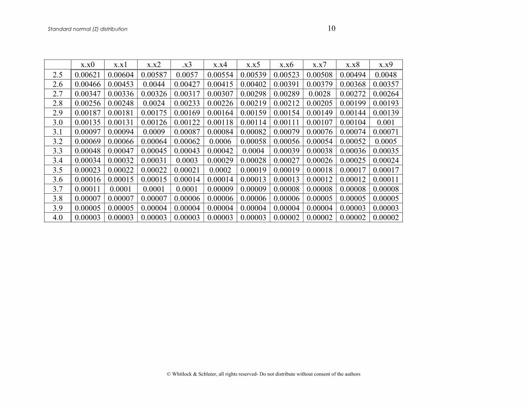
Standard normal (Z) distribution 10


x.x0 x.x1 x.x2 .x3 x.x4 x.x5 x.x6 x.x7 x.x8 x.x92.5 0.00621 0.00604 0.00587 0.0057 0.00554 0.00539 0.00523 0.00508 0.00494 0.00482.6 0.00466 0.00453 0.0044 0.00427 0.00415 0.00402 0.00391 0.00379 0.00368 0.003572.7 0.00347 0.00336 0.00326 0.00317 0.00307 0.00298 0.00289 0.0028 0.00272 0.002642.8 0.00256 0.00248 0.0024 0.00233 0.00226 0.00219 0.00212 0.00205 0.00199 0.001932.9 0.00187 0.00181 0.00175 0.00169 0.00164 0.00159 0.00154 0.00149 0.00144 0.001393.0 0.00135 0.00131 0.00126 0.00122 0.00118 0.00114 0.00111 0.00107 0.00104 0.0013.1 0.00097 0.00094 0.0009 0.00087 0.00084 0.00082 0.00079 0.00076 0.00074 0.000713.2 0.00069 0.00066 0.00064 0.00062 0.0006 0.00058 0.00056 0.00054 0.00052 0.00053.3 0.00048 0.00047 0.00045 0.00043 0.00042 0.0004 0.00039 0.00038 0.00036 0.000353.4 0.00034 0.00032 0.00031 0.0003 0.00029 0.00028 0.00027 0.00026 0.00025 0.000243.5 0.00023 0.00022 0.00022 0.00021 0.0002 0.00019 0.00019 0.00018 0.00017 0.000173.6 0.00016 0.00015 0.00015 0.00014 0.00014 0.00013 0.00013 0.00012 0.00012 0.000113.7 0.00011 0.0001 0.0001 0.0001 0.00009 0.00009 0.00008 0.00008 0.00008 0.000083.8 0.00007 0.00007 0.00007 0.00006 0.00006 0.00006 0.00006 0.00005 0.00005 0.000053.9 0.00005 0.00005 0.00004 0.00004 0.00004 0.00004 0.00004 0.00004 0.00003 0.000034.0 0.00003 0.00003 0.00003 0.00003 0.00003 0.00003 0.00002 0.00002 0.00002 0.00002


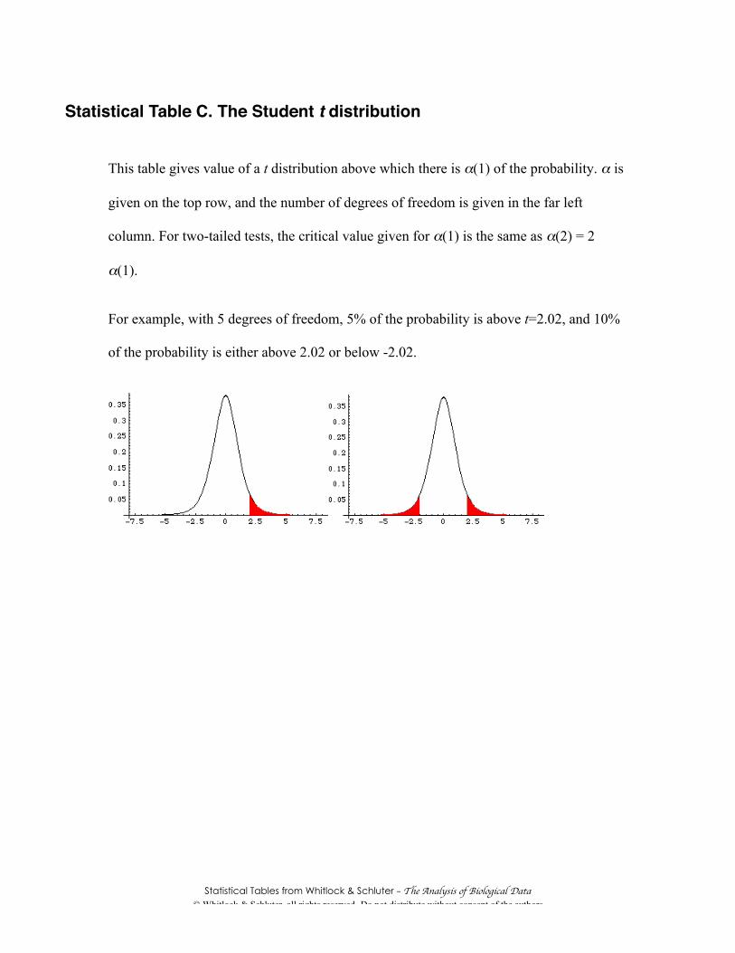
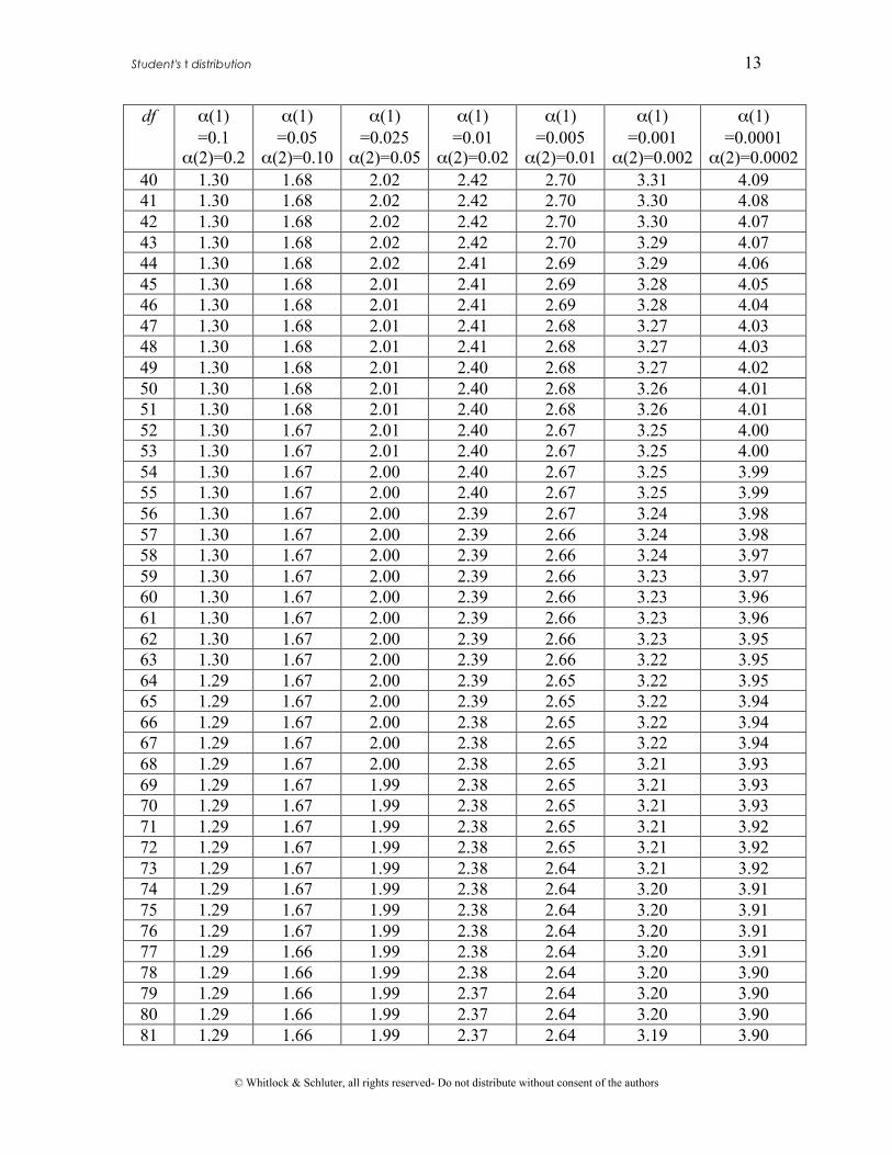
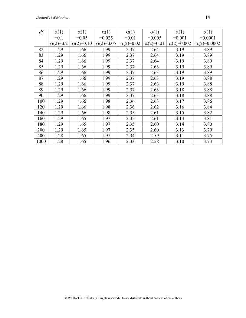
Statistical Table C. The Student t distribution

This table gives value of a t distribution above which there is α(1) of the probability. α is

given on the top row, and the number of degrees of freedom is given in the far left

column. For two-tailed tests, the critical value given for α(1) is the same as α(2) = 2

α(1).

For example, with 5 degrees of freedom, 5% of the probability is above t=2.02, and 10%

of the probability is either above 2.02 or below -2.02.

Student's t distribution 12


df α(1)=0.1

α(2)=0.2

α(1)=0.05

α(2)=0.10

α(1)=0.025

α(2)=0.05

α(1)=0.01

α(2)=0.02

α(1)=0.005

α(2)=0.01

α(1)=0.001

α(2)=0.002

α(1)=0.0001

α(2)=0.00021 3.08 6.31 12.71 31.82 63.66 318.31 3183.12 1.89 2.92 4.30 6.96 9.92 22.33 70.703 1.64 2.35 3.18 4.54 5.84 10.21 22.204 1.53 2.13 2.78 3.75 4.60 7.17 13.035 1.48 2.02 2.57 3.36 4.03 5.89 9.686 1.44 1.94 2.45 3.14 3.71 5.21 8.027 1.41 1.89 2.36 3.00 3.50 4.79 7.068 1.40 1.86 2.31 2.90 3.36 4.50 6.449 1.38 1.83 2.26 2.82 3.25 4.30 6.0110 1.37 1.81 2.23 2.76 3.17 4.14 5.6911 1.36 1.80 2.20 2.72 3.11 4.02 5.4512 1.36 1.78 2.18 2.68 3.05 3.93 5.2613 1.35 1.77 2.16 2.65 3.01 3.85 5.1114 1.35 1.76 2.14 2.62 2.98 3.79 4.9915 1.34 1.75 2.13 2.60 2.95 3.73 4.8816 1.34 1.75 2.12 2.58 2.92 3.69 4.7917 1.33 1.74 2.11 2.57 2.90 3.65 4.7118 1.33 1.73 2.10 2.55 2.88 3.61 4.6519 1.33 1.73 2.09 2.54 2.86 3.58 4.5920 1.33 1.72 2.09 2.53 2.85 3.55 4.5421 1.32 1.72 2.08 2.52 2.83 3.53 4.4922 1.32 1.72 2.07 2.51 2.82 3.50 4.4523 1.32 1.71 2.07 2.50 2.81 3.48 4.4224 1.32 1.71 2.06 2.49 2.80 3.47 4.3825 1.32 1.71 2.06 2.49 2.79 3.45 4.3526 1.31 1.71 2.06 2.48 2.78 3.43 4.3227 1.31 1.70 2.05 2.47 2.77 3.42 4.3028 1.31 1.70 2.05 2.47 2.76 3.41 4.2829 1.31 1.70 2.05 2.46 2.76 3.40 4.2530 1.31 1.70 2.04 2.46 2.75 3.39 4.2331 1.31 1.70 2.04 2.45 2.74 3.37 4.2232 1.31 1.69 2.04 2.45 2.74 3.37 4.2033 1.31 1.69 2.03 2.44 2.73 3.36 4.1834 1.31 1.69 2.03 2.44 2.73 3.35 4.1735 1.31 1.69 2.03 2.44 2.72 3.34 4.1536 1.31 1.69 2.03 2.43 2.72 3.33 4.1437 1.30 1.69 2.03 2.43 2.72 3.33 4.1338 1.30 1.69 2.02 2.43 2.71 3.32 4.1239 1.30 1.68 2.02 2.43 2.71 3.31 4.10



df α(1)=0.1

α(2)=0.2

α(1)=0.05

α(2)=0.10

α(1)=0.025

α(2)=0.05

α(1)=0.01

α(2)=0.02

α(1)=0.005

α(2)=0.01

α(1)=0.001

α(2)=0.002

α(1)=0.0001

α(2)=0.000240 1.30 1.68 2.02 2.42 2.70 3.31 4.0941 1.30 1.68 2.02 2.42 2.70 3.30 4.0842 1.30 1.68 2.02 2.42 2.70 3.30 4.0743 1.30 1.68 2.02 2.42 2.70 3.29 4.0744 1.30 1.68 2.02 2.41 2.69 3.29 4.0645 1.30 1.68 2.01 2.41 2.69 3.28 4.0546 1.30 1.68 2.01 2.41 2.69 3.28 4.0447 1.30 1.68 2.01 2.41 2.68 3.27 4.0348 1.30 1.68 2.01 2.41 2.68 3.27 4.0349 1.30 1.68 2.01 2.40 2.68 3.27 4.0250 1.30 1.68 2.01 2.40 2.68 3.26 4.0151 1.30 1.68 2.01 2.40 2.68 3.26 4.0152 1.30 1.67 2.01 2.40 2.67 3.25 4.0053 1.30 1.67 2.01 2.40 2.67 3.25 4.0054 1.30 1.67 2.00 2.40 2.67 3.25 3.9955 1.30 1.67 2.00 2.40 2.67 3.25 3.9956 1.30 1.67 2.00 2.39 2.67 3.24 3.9857 1.30 1.67 2.00 2.39 2.66 3.24 3.9858 1.30 1.67 2.00 2.39 2.66 3.24 3.9759 1.30 1.67 2.00 2.39 2.66 3.23 3.9760 1.30 1.67 2.00 2.39 2.66 3.23 3.9661 1.30 1.67 2.00 2.39 2.66 3.23 3.9662 1.30 1.67 2.00 2.39 2.66 3.23 3.9563 1.30 1.67 2.00 2.39 2.66 3.22 3.9564 1.29 1.67 2.00 2.39 2.65 3.22 3.9565 1.29 1.67 2.00 2.39 2.65 3.22 3.9466 1.29 1.67 2.00 2.38 2.65 3.22 3.9467 1.29 1.67 2.00 2.38 2.65 3.22 3.9468 1.29 1.67 2.00 2.38 2.65 3.21 3.9369 1.29 1.67 1.99 2.38 2.65 3.21 3.9370 1.29 1.67 1.99 2.38 2.65 3.21 3.9371 1.29 1.67 1.99 2.38 2.65 3.21 3.9272 1.29 1.67 1.99 2.38 2.65 3.21 3.9273 1.29 1.67 1.99 2.38 2.64 3.21 3.9274 1.29 1.67 1.99 2.38 2.64 3.20 3.9175 1.29 1.67 1.99 2.38 2.64 3.20 3.9176 1.29 1.67 1.99 2.38 2.64 3.20 3.9177 1.29 1.66 1.99 2.38 2.64 3.20 3.9178 1.29 1.66 1.99 2.38 2.64 3.20 3.9079 1.29 1.66 1.99 2.37 2.64 3.20 3.9080 1.29 1.66 1.99 2.37 2.64 3.20 3.9081 1.29 1.66 1.99 2.37 2.64 3.19 3.90



df α(1)=0.1

α(2)=0.2

α(1)=0.05

α(2)=0.10

α(1)=0.025

α(2)=0.05

α(1)=0.01

α(2)=0.02

α(1)=0.005

α(2)=0.01

α(1)=0.001

α(2)=0.002

α(1)=0.0001

α(2)=0.000282 1.29 1.66 1.99 2.37 2.64 3.19 3.8983 1.29 1.66 1.99 2.37 2.64 3.19 3.8984 1.29 1.66 1.99 2.37 2.64 3.19 3.8985 1.29 1.66 1.99 2.37 2.63 3.19 3.8986 1.29 1.66 1.99 2.37 2.63 3.19 3.8987 1.29 1.66 1.99 2.37 2.63 3.19 3.8888 1.29 1.66 1.99 2.37 2.63 3.19 3.8889 1.29 1.66 1.99 2.37 2.63 3.18 3.8890 1.29 1.66 1.99 2.37 2.63 3.18 3.88

100 1.29 1.66 1.98 2.36 2.63 3.17 3.86120 1.29 1.66 1.98 2.36 2.62 3.16 3.84140 1.29 1.66 1.98 2.35 2.61 3.15 3.82160 1.29 1.65 1.97 2.35 2.61 3.14 3.81180 1.29 1.65 1.97 2.35 2.60 3.14 3.80200 1.29 1.65 1.97 2.35 2.60 3.13 3.79400 1.28 1.65 1.97 2.34 2.59 3.11 3.751000 1.28 1.65 1.96 2.33 2.58 3.10 3.73


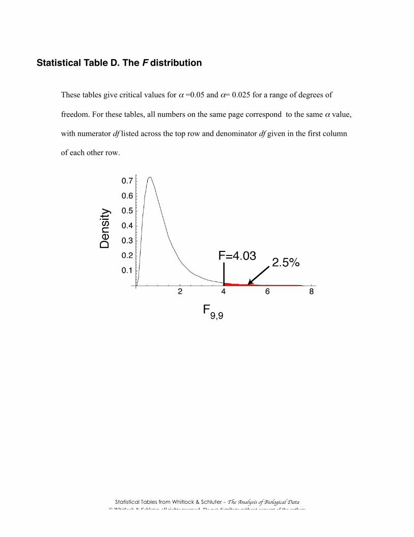
Statistical Table D. The F distribution

These tables give critical values for α =0.05 and α= 0.025 for a range of degrees of

freedom. For these tables, all numbers on the same page correspond to the same α value,

with numerator df listed across the top row and denominator df given in the first column

of each other row.

F distribution 16


Critical value of F, α(1)=0.05, α(2)=0.10

Numerator dfden.df

1 2 3 4 5 6 7 8 9 10

1 161.45 199.50 215.71 224.58 230.16 233.99 236.77 238.88 240.54 241.882 18.51 19.00 19.16 19.25 19.30 19.33 19.35 19.37 19.38 19.403 10.13 9.55 9.28 9.12 9.01 8.94 8.89 8.85 8.81 8.794 7.71 6.94 6.59 6.39 6.26 6.16 6.09 6.04 6.00 5.965 6.61 5.79 5.41 5.19 5.05 4.95 4.88 4.82 4.77 4.746 5.99 5.14 4.76 4.53 4.39 4.28 4.21 4.15 4.10 4.067 5.59 4.74 4.35 4.12 3.97 3.87 3.79 3.73 3.68 3.648 5.32 4.46 4.07 3.84 3.69 3.58 3.50 3.44 3.39 3.359 5.12 4.26 3.86 3.63 3.48 3.37 3.29 3.23 3.18 3.14

10 4.96 4.10 3.71 3.48 3.33 3.22 3.14 3.07 3.02 2.9811 4.84 3.98 3.59 3.36 3.20 3.09 3.01 2.95 2.90 2.8512 4.75 3.89 3.49 3.26 3.11 3.00 2.91 2.85 2.80 2.7513 4.67 3.81 3.41 3.18 3.03 2.92 2.83 2.77 2.71 2.6714 4.60 3.74 3.34 3.11 2.96 2.85 2.76 2.70 2.65 2.6015 4.54 3.68 3.29 3.06 2.90 2.79 2.71 2.64 2.59 2.5416 4.49 3.63 3.24 3.01 2.85 2.74 2.66 2.59 2.54 2.4917 4.45 3.59 3.20 2.96 2.81 2.70 2.61 2.55 2.49 2.4518 4.41 3.55 3.16 2.93 2.77 2.66 2.58 2.51 2.46 2.4119 4.38 3.52 3.13 2.90 2.74 2.63 2.54 2.48 2.42 2.3820 4.35 3.49 3.10 2.87 2.71 2.60 2.51 2.45 2.39 2.3521 4.32 3.47 3.07 2.84 2.68 2.57 2.49 2.42 2.37 2.3222 4.30 3.44 3.05 2.82 2.66 2.55 2.46 2.40 2.34 2.3023 4.28 3.42 3.03 2.80 2.64 2.53 2.44 2.37 2.32 2.2724 4.26 3.40 3.01 2.78 2.62 2.51 2.42 2.36 2.30 2.2525 4.24 3.39 2.99 2.76 2.60 2.49 2.40 2.34 2.28 2.2426 4.23 3.37 2.98 2.74 2.59 2.47 2.39 2.32 2.27 2.2227 4.21 3.35 2.96 2.73 2.57 2.46 2.37 2.31 2.25 2.2028 4.20 3.34 2.95 2.71 2.56 2.45 2.36 2.29 2.24 2.1929 4.18 3.33 2.93 2.70 2.55 2.43 2.35 2.28 2.22 2.1830 4.17 3.32 2.92 2.69 2.53 2.42 2.33 2.27 2.21 2.1640 4.08 3.23 2.84 2.61 2.45 2.34 2.25 2.18 2.12 2.0850 4.03 3.18 2.79 2.56 2.40 2.29 2.20 2.13 2.07 2.0360 4.00 3.15 2.76 2.53 2.37 2.25 2.17 2.10 2.04 1.9970 3.98 3.13 2.74 2.50 2.35 2.23 2.14 2.07 2.02 1.9780 3.96 3.11 2.72 2.49 2.33 2.21 2.13 2.06 2.00 1.9590 3.95 3.10 2.71 2.47 2.32 2.20 2.11 2.04 1.99 1.94100 3.94 3.09 2.70 2.46 2.31 2.19 2.10 2.03 1.97 1.93200 3.89 3.04 2.65 2.42 2.26 2.14 2.06 1.98 1.93 1.88400 3.86 3.02 2.63 2.39 2.24 2.12 2.03 1.96 1.90 1.85

F distribution 17


Critical value of F, α(1)=0.05, α(2)=0.10, continued

Numerator dfden.df

12 15 20 30 40 60 100 200 400 1000

1 243.91 245.95 248.01 250.10 251.14 252.20 253.04 253.68 254.00 254.192 19.41 19.43 19.45 19.46 19.47 19.48 19.49 19.49 19.49 19.493 8.74 8.70 8.66 8.62 8.59 8.57 8.55 8.54 8.53 8.534 5.91 5.86 5.80 5.75 5.72 5.69 5.66 5.65 5.64 5.635 4.68 4.62 4.56 4.50 4.46 4.43 4.41 4.39 4.38 4.376 4.00 3.94 3.87 3.81 3.77 3.74 3.71 3.69 3.68 3.677 3.57 3.51 3.44 3.38 3.34 3.30 3.27 3.25 3.24 3.238 3.28 3.22 3.15 3.08 3.04 3.01 2.97 2.95 2.94 2.939 3.07 3.01 2.94 2.86 2.83 2.79 2.76 2.73 2.72 2.71

10 2.91 2.85 2.77 2.70 2.66 2.62 2.59 2.56 2.55 2.5411 2.79 2.72 2.65 2.57 2.53 2.49 2.46 2.43 2.42 2.4112 2.69 2.62 2.54 2.47 2.43 2.38 2.35 2.32 2.31 2.3013 2.60 2.53 2.46 2.38 2.34 2.30 2.26 2.23 2.22 2.2114 2.53 2.46 2.39 2.31 2.27 2.22 2.19 2.16 2.15 2.1415 2.48 2.40 2.33 2.25 2.20 2.16 2.12 2.10 2.08 2.0716 2.42 2.35 2.28 2.19 2.15 2.11 2.07 2.04 2.02 2.0217 2.38 2.31 2.23 2.15 2.10 2.06 2.02 1.99 1.98 1.9718 2.34 2.27 2.19 2.11 2.06 2.02 1.98 1.95 1.93 1.9219 2.31 2.23 2.16 2.07 2.03 1.98 1.94 1.91 1.89 1.8820 2.28 2.20 2.12 2.04 1.99 1.95 1.91 1.88 1.86 1.8521 2.25 2.18 2.10 2.01 1.96 1.92 1.88 1.84 1.83 1.8222 2.23 2.15 2.07 1.98 1.94 1.89 1.85 1.82 1.80 1.7923 2.20 2.13 2.05 1.96 1.91 1.86 1.82 1.79 1.77 1.7624 2.18 2.11 2.03 1.94 1.89 1.84 1.80 1.77 1.75 1.7425 2.16 2.09 2.01 1.92 1.87 1.82 1.78 1.75 1.73 1.7226 2.15 2.07 1.99 1.90 1.85 1.80 1.76 1.73 1.71 1.7027 2.13 2.06 1.97 1.88 1.84 1.79 1.74 1.71 1.69 1.6828 2.12 2.04 1.96 1.87 1.82 1.77 1.73 1.69 1.67 1.6629 2.10 2.03 1.94 1.85 1.81 1.75 1.71 1.67 1.66 1.6530 2.09 2.01 1.93 1.84 1.79 1.74 1.70 1.66 1.64 1.6340 2.00 1.92 1.84 1.74 1.69 1.64 1.59 1.55 1.53 1.5250 1.95 1.87 1.78 1.69 1.63 1.58 1.52 1.48 1.46 1.4560 1.92 1.84 1.75 1.65 1.59 1.53 1.48 1.44 1.41 1.4070 1.89 1.81 1.72 1.62 1.57 1.50 1.45 1.40 1.38 1.3680 1.88 1.79 1.70 1.60 1.54 1.48 1.43 1.38 1.35 1.3490 1.86 1.78 1.69 1.59 1.53 1.46 1.41 1.36 1.33 1.31100 1.85 1.77 1.68 1.57 1.52 1.45 1.39 1.34 1.31 1.30200 1.80 1.72 1.62 1.52 1.46 1.39 1.32 1.26 1.23 1.21400 1.78 1.69 1.60 1.49 1.42 1.35 1.28 1.22 1.18 1.15

F distribution 18


Critical value of F, α(1)=0.025, α(2)=0.05

Numerator dfden.df

1 2 3 4 5 6 7 8 9 10

1 647.79 799.50 864.16 899.58 921.85 937.11 948.22 956.66 963.28 968.632 38.51 39.00 39.17 39.25 39.30 3 9 . 3

339.36 39.37 39.39 39.40

3 17.44 16.04 15.44 15.10 14.88 14.73 14.62 14.54 14.47 14.424 12.22 10.65 9.98 9.60 9.36 9.20 9.07 8.98 8.90 8.845 10.01 8.43 7.76 7.39 7.15 6.98 6.85 6.76 6.68 6.626 8.81 7.26 6.60 6.23 5.99 5.82 5.70 5.60 5.52 5.467 8.07 6.54 5.89 5.52 5.29 5.12 4.99 4.90 4.82 4.768 7.57 6.06 5.42 5.05 4.82 4.65 4.53 4.43 4.36 4.309 7.21 5.71 5.08 4.72 4.48 4.32 4.20 4.10 4.03 3.96

10 6.94 5.46 4.83 4.47 4.24 4.07 3.95 3.85 3.78 3.7211 6.72 5.26 4.63 4.28 4.04 3.88 3.76 3.66 3.59 3.5312 6.55 5.10 4.47 4.12 3.89 3.73 3.61 3.51 3.44 3.3713 6.41 4.97 4.35 4.00 3.77 3.60 3.48 3.39 3.31 3.2514 6.30 4.86 4.24 3.89 3.66 3.50 3.38 3.29 3.21 3.1515 6.20 4.77 4.15 3.80 3.58 3.41 3.29 3.20 3.12 3.0616 6.12 4.69 4.08 3.73 3.50 3.34 3.22 3.12 3.05 2.9917 6.04 4.62 4.01 3.66 3.44 3.28 3.16 3.06 2.98 2.9218 5.98 4.56 3.95 3.61 3.38 3.22 3.10 3.01 2.93 2.8719 5.92 4.51 3.90 3.56 3.33 3.17 3.05 2.96 2.88 2.8220 5.87 4.46 3.86 3.51 3.29 3.13 3.01 2.91 2.84 2.7721 5.83 4.42 3.82 3.48 3.25 3.09 2.97 2.87 2.80 2.7322 5.79 4.38 3.78 3.44 3.22 3.05 2.93 2.84 2.76 2.7023 5.75 4.35 3.75 3.41 3.18 3.02 2.90 2.81 2.73 2.6724 5.72 4.32 3.72 3.38 3.15 2.99 2.87 2.78 2.70 2.6425 5.69 4.29 3.69 3.35 3.13 2.97 2.85 2.75 2.68 2.6126 5.66 4.27 3.67 3.33 3.10 2.94 2.82 2.73 2.65 2.5927 5.63 4.24 3.65 3.31 3.08 2.92 2.80 2.71 2.63 2.5728 5.61 4.22 3.63 3.29 3.06 2.90 2.78 2.69 2.61 2.5529 5.59 4.20 3.61 3.27 3.04 2.88 2.76 2.67 2.59 2.5330 5.57 4.18 3.59 3.25 3.03 2.87 2.75 2.65 2.57 2.5140 5.42 4.05 3.46 3.13 2.90 2.74 2.62 2.53 2.45 2.3950 5.34 3.97 3.39 3.05 2.83 2.67 2.55 2.46 2.38 2.3260 5.29 3.93 3.34 3.01 2.79 2.63 2.51 2.41 2.33 2.2770 5.25 3.89 3.31 2.97 2.75 2.59 2.47 2.38 2.30 2.2480 5.22 3.86 3.28 2.95 2.73 2.57 2.45 2.35 2.28 2.2190 5.20 3.84 3.26 2.93 2.71 2.55 2.43 2.34 2.26 2.19100 5.18 3.83 3.25 2.92 2.70 2.54 2.42 2.32 2.24 2.18200 5.10 3.76 3.18 2.85 2.63 2.47 2.35 2.26 2.18 2.11400 5.06 3.72 3.15 2.82 2.60 2.44 2.32 2.22 2.15 2.08

F distribution 19


Critical value of F, α(1)=0.025, α(2)=0.05, continued

Numerator dfden.df

12 15 20 30 40 60 100 200 400 1000

1 976.71 984.87 993.10 1001.40 1005.60 1009.80 1013.20 1015.70 1017.00 1017.802 39.41 39.43 39.45 39.46 39.47 39.48 39.49 39.49 39.50 39.503 14.34 14.25 14.17 14.08 14.04 13.99 13.96 13.93 13.92 13.914 8.75 8.66 8.56 8.46 8.41 8.36 8.32 8.29 8.27 8.265 6.52 6.43 6.33 6.23 6.18 6.12 6.08 6.05 6.03 6.026 5.37 5.27 5.17 5.07 5.01 4.96 4.92 4.88 4.87 4.867 4.67 4.57 4.47 4.36 4.31 4.25 4.21 4.18 4.16 4.158 4.20 4.10 4.00 3.89 3.84 3.78 3.74 3.70 3.69 3.689 3.87 3.77 3.67 3.56 3.51 3.45 3.40 3.37 3.35 3.34

10 3.62 3.52 3.42 3.31 3.26 3.20 3.15 3.12 3.10 3.0911 3.43 3.33 3.23 3.12 3.06 3.00 2.96 2.92 2.90 2.8912 3.28 3.18 3.07 2.96 2.91 2.85 2.80 2.76 2.74 2.7313 3.15 3.05 2.95 2.84 2.78 2.72 2.67 2.63 2.61 2.6014 3.05 2.95 2.84 2.73 2.67 2.61 2.56 2.53 2.51 2.5015 2.96 2.86 2.76 2.64 2.59 2.52 2.47 2.44 2.42 2.4016 2.89 2.79 2.68 2.57 2.51 2.45 2.40 2.36 2.34 2.3217 2.82 2.72 2.62 2.50 2.44 2.38 2.33 2.29 2.27 2.2618 2.77 2.67 2.56 2.44 2.38 2.32 2.27 2.23 2.21 2.2019 2.72 2.62 2.51 2.39 2.33 2.27 2.22 2.18 2.15 2.1420 2.68 2.57 2.46 2.35 2.29 2.22 2.17 2.13 2.11 2.0921 2.64 2.53 2.42 2.31 2.25 2.18 2.13 2.09 2.06 2.0522 2.60 2.50 2.39 2.27 2.21 2.14 2.09 2.05 2.03 2.0123 2.57 2.47 2.36 2.24 2.18 2.11 2.06 2.01 1.99 1.9824 2.54 2.44 2.33 2.21 2.15 2.08 2.02 1.98 1.96 1.9425 2.51 2.41 2.30 2.18 2.12 2.05 2.00 1.95 1.93 1.9126 2.49 2.39 2.28 2.16 2.09 2.03 1.97 1.92 1.90 1.8927 2.47 2.36 2.25 2.13 2.07 2.00 1.94 1.90 1.88 1.8628 2.45 2.34 2.23 2.11 2.05 1.98 1.92 1.88 1.85 1.8429 2.43 2.32 2.21 2.09 2.03 1.96 1.90 1.86 1.83 1.8230 2.41 2.31 2.20 2.07 2.01 1.94 1.88 1.84 1.81 1.8040 2.29 2.18 2.07 1.94 1.88 1.80 1.74 1.69 1.66 1.6550 2.22 2.11 1.99 1.87 1.80 1.72 1.66 1.60 1.57 1.5660 2.17 2.06 1.94 1.82 1.74 1.67 1.60 1.54 1.51 1.4970 2.14 2.03 1.91 1.78 1.71 1.63 1.56 1.50 1.47 1.4580 2.11 2.00 1.88 1.75 1.68 1.60 1.53 1.47 1.43 1.4190 2.09 1.98 1.86 1.73 1.66 1.58 1.50 1.44 1.41 1.39100 2.08 1.97 1.85 1.71 1.64 1.56 1.48 1.42 1.39 1.36200 2.01 1.90 1.78 1.64 1.56 1.47 1.39 1.32 1.28 1.25400 1.98 1.87 1.74 1.60 1.52 1.43 1.35 1.27 1.22 1.18


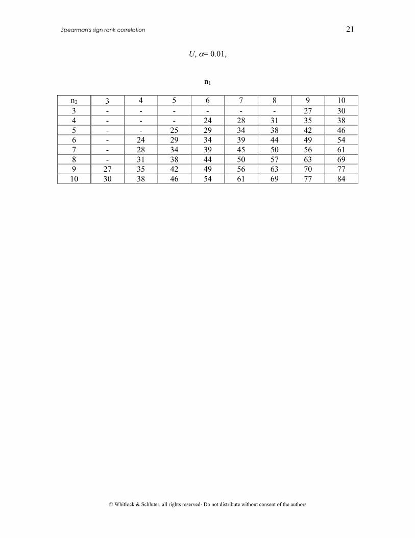
Statistical table E: Mann-Whitney U distribution

When the sample size increases above 10 for either sample, the Z approximation given in

the text works reasonably well. Here we give reduced version of the tables for the Mann-

Whitney U distribution. Test statistics larger than those given in the table will be

significant at the given a level. n1 and n2refer to the sample sizes of the two samples. "-"

means that it is not possible to reject a null hypothesis with that α with those sample

sizes.

U, α= 0.05

n1

n2 3 4 5 6 7 8 9 103 - - 15 17 20 22 25 274 - 16 19 22 25 28 32 355 15 19 23 27 30 34 38 426 17 22 27 31 36 40 44 497 20 25 30 36 41 46 51 568 22 28 34 40 46 51 57 639 25 32 38 44 51 57 64 7010 27 35 42 49 56 63 70 77

Spearman's sign rank correlation 21


U, α= 0.01,

n1

n2 3 4 5 6 7 8 9 103 - - - - - - 27 304 - - - 24 28 31 35 385 - - 25 29 34 38 42 466 - 24 29 34 39 44 49 547 - 28 34 39 45 50 56 618 - 31 38 44 50 57 63 699 27 35 42 49 56 63 70 7710 30 38 46 54 61 69 77 84


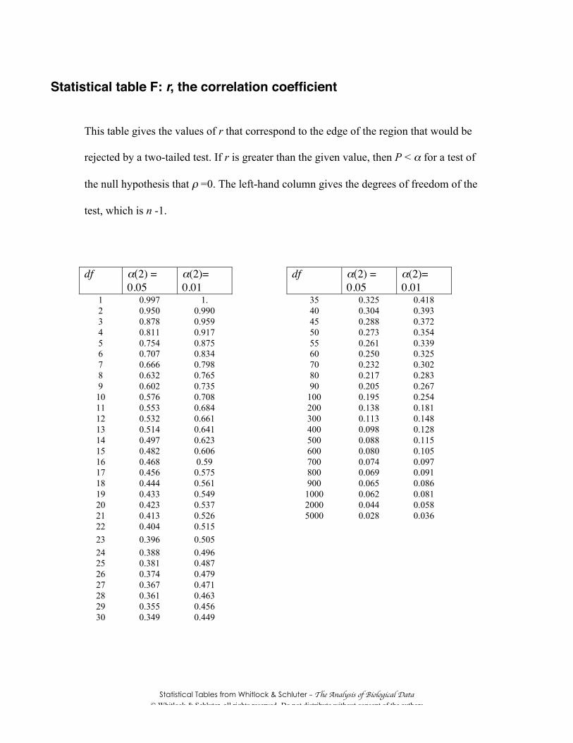
Statistical table F: r, the correlation coefficient

This table gives the values of r that correspond to the edge of the region that would be

rejected by a two-tailed test. If r is greater than the given value, then P < α for a test of

the null hypothesis that ρ =0. The left-hand column gives the degrees of freedom of the

test, which is n -1.

df α(2) =0.05

α(2)=0.01

df α(2) =0.05

α(2)=0.01

1 0.997 1. 35 0.325 0.4182 0.950 0.990 40 0.304 0.3933 0.878 0.959 45 0.288 0.3724 0.811 0.917 50 0.273 0.3545 0.754 0.875 55 0.261 0.3396 0.707 0.834 60 0.250 0.3257 0.666 0.798 70 0.232 0.3028 0.632 0.765 80 0.217 0.2839 0.602 0.735 90 0.205 0.26710 0.576 0.708 100 0.195 0.25411 0.553 0.684 200 0.138 0.18112 0.532 0.661 300 0.113 0.14813 0.514 0.641 400 0.098 0.12814 0.497 0.623 500 0.088 0.11515 0.482 0.606 600 0.080 0.10516 0.468 0.59 700 0.074 0.09717 0.456 0.575 800 0.069 0.09118 0.444 0.561 900 0.065 0.08619 0.433 0.549 1000 0.062 0.08120 0.423 0.537 2000 0.044 0.05821 0.413 0.526 5000 0.028 0.03622 0.404 0.51523 0.396 0.50524 0.388 0.49625 0.381 0.48726 0.374 0.47927 0.367 0.47128 0.361 0.46329 0.355 0.45630 0.349 0.449


Statistical Table G: Tukey-Kramer critical values at α = 0.05

Number of groups (k)dferror 2 3 4 5 6 7 8 9 10 11 12 13 14 1510 2.23 2.74 3.06 3.29 3.47 3.62 3.75 3.86 3.96 4.05 4.12 4.20 4.26 4.3211 2.20 2.70 3.01 3.23 3.41 3.56 3.68 3.79 3.88 3.96 4.04 4.11 4.17 4.2312 2.18 2.67 2.97 3.19 3.36 3.50 3.62 3.72 3.81 3.90 3.97 4.04 4.10 4.1613 2.16 2.64 2.94 3.15 3.32 3.45 3.57 3.67 3.76 3.84 3.91 3.98 4.04 4.0914 2.14 2.62 2.91 3.12 3.28 3.41 3.53 3.63 3.72 3.79 3.86 3.93 3.99 4.0415 2.13 2.60 2.88 3.09 3.25 3.38 3.49 3.59 3.68 3.75 3.82 3.88 3.94 3.9916 2.12 2.58 2.86 3.06 3.22 3.35 3.46 3.56 3.64 3.72 3.78 3.85 3.90 3.9517 2.11 2.57 2.84 3.04 3.20 3.33 3.44 3.53 3.61 3.69 3.75 3.81 3.87 3.9218 2.10 2.55 2.83 3.02 3.18 3.30 3.41 3.50 3.59 3.66 3.72 3.78 3.84 3.8919 2.09 2.54 2.81 3.01 3.16 3.16 3.39 3.48 3.56 3.63 3.70 3.76 3.81 3.8620 2.09 2.53 2.80 2.99 3.14 3.27 3.37 3.46 3.54 3.61 3.68 3.73 3.79 3.8421 2.08 2.52 2.79 2.98 3.13 3.25 3.35 3.44 3.52 3.59 3.66 3.71 3.77 3.8222 2.07 2.51 2.78 2.97 3.12 3.24 3.34 3.43 3.51 3.57 3.64 3.69 3.75 3.8023 2.07 2.50 2.77 2.96 3.10 3.22 3.32 3.41 3.49 3.56 3.62 3.68 3.73 3.7824 2.06 2.50 2.76 2.95 3.09 3.21 3.31 3.40 3.48 3.54 3.61 3.66 3.71 3.7625 2.06 2.49 2.75 2.94 3.08 3.20 3.30 3.39 3.46 3.53 3.59 3.65 3.70 3.7526 2.06 2.48 2.74 2.93 3.07 3.19 3.29 3.38 3.45 3.52 3.58 3.63 3.68 3.7327 2.05 2.48 2.74 2.92 3.06 3.18 3.28 3.36 3.44 3.51 3.57 3.62 3.67 3.7228 2.05 2.47 2.73 2.91 3.06 3.17 3.27 3.35 3.43 3.50 3.56 3.61 3.66 3.7129 2.05 2.47 2.72 2.91 3.05 3.16 3.26 3.35 3.42 3.49 3.55 3.60 3.65 3.7030 2.04 2.46 2.72 2.90 3.04 3.16 3.25 3.34 3.41 3.48 3.54 3.59 3.64 3.6831 2.04 2.46 2.71 2.89 3.04 3.15 3.25 3.33 3.40 3.47 3.53 3.58 3.63 3.6832 2.04 2.46 2.71 2.89 3.03 3.14 3.24 3.32 3.40 3.46 3.52 3.57 3.62 3.6733 2.03 2.45 2.70 2.88 3.02 3.14 3.23 3.32 3.39 3.45 3.51 3.56 3.61 3.6634 2.03 2.45 2.70 2.88 3.02 3.13 3.23 3.31 3.38 3.45 3.50 3.56 3.60 3.6535 2.03 2.45 2.70 2.88 3.01 3.13 3.22 3.30 3.37 3.44 3.50 3.55 3.60 3.6436 2.03 2.44 2.69 2.87 3.01 3.12 3.22 3.30 3.37 3.43 3.49 3.54 3.59 3.6437 2.03 2.44 2.69 2.87 3.00 3.12 3.21 3.29 3.36 3.43 3.48 3.54 3.58 3.6338 2.02 2.44 2.69 2.86 3.00 3.11 3.21 3.29 3.36 3.42 3.48 3.53 3.58 3.6239 2.02 2.44 2.68 2.86 3.00 3.11 3.20 3.28 3.35 3.42 3.47 3.52 3.57 3.6240 2.02 2.43 2.68 2.86 2.99 3.10 3.20 3.28 3.35 3.41 3.47 3.52 3.57 3.6141 2.02 2.43 2.68 2.85 2.99 3.10 3.19 3.27 3.34 3.41 3.46 3.51 3.56 3.6042 2.02 2.43 2.67 2.85 2.99 3.10 3.19 3.27 3.34 3.40 3.46 3.51 3.56 3.6043 2.02 2.43 2.67 2.85 2.98 3.09 3.18 3.26 3.33 3.40 3.45 3.50 3.55 3.5944 2.02 2.43 2.67 2.84 2.98 3.09 3.18 3.26 3.33 3.39 3.45 3.50 3.55 3.5945 2.01 2.42 2.67 2.84 2.98 3.09 3.18 3.26 3.33 3.39 3.44 3.50 3.54 3.5946 2.01 2.42 2.67 2.84 2.97 3.08 3.17 3.25 3.32 3.39 3.44 3.49 3.54 3.5847 2.01 2.42 2.66 2.84 2.97 3.08 3.17 3.25 3.32 3.38 3.44 3.49 3.53 3.5848 2.01 2.42 2.66 2.83 2.97 3.08 3.17 3.25 3.32 3.38 3.43 3.48 3.53 3.5749 2.01 2.42 2.66 2.83 2.97 3.07 3.17 3.24 3.31 3.37 3.43 3.48 3.53 3.5750 2.01 2.42 2.66 2.83 2.96 3.07 3.16 3.24 3.31 3.37 3.43 3.48 3.52 3.57


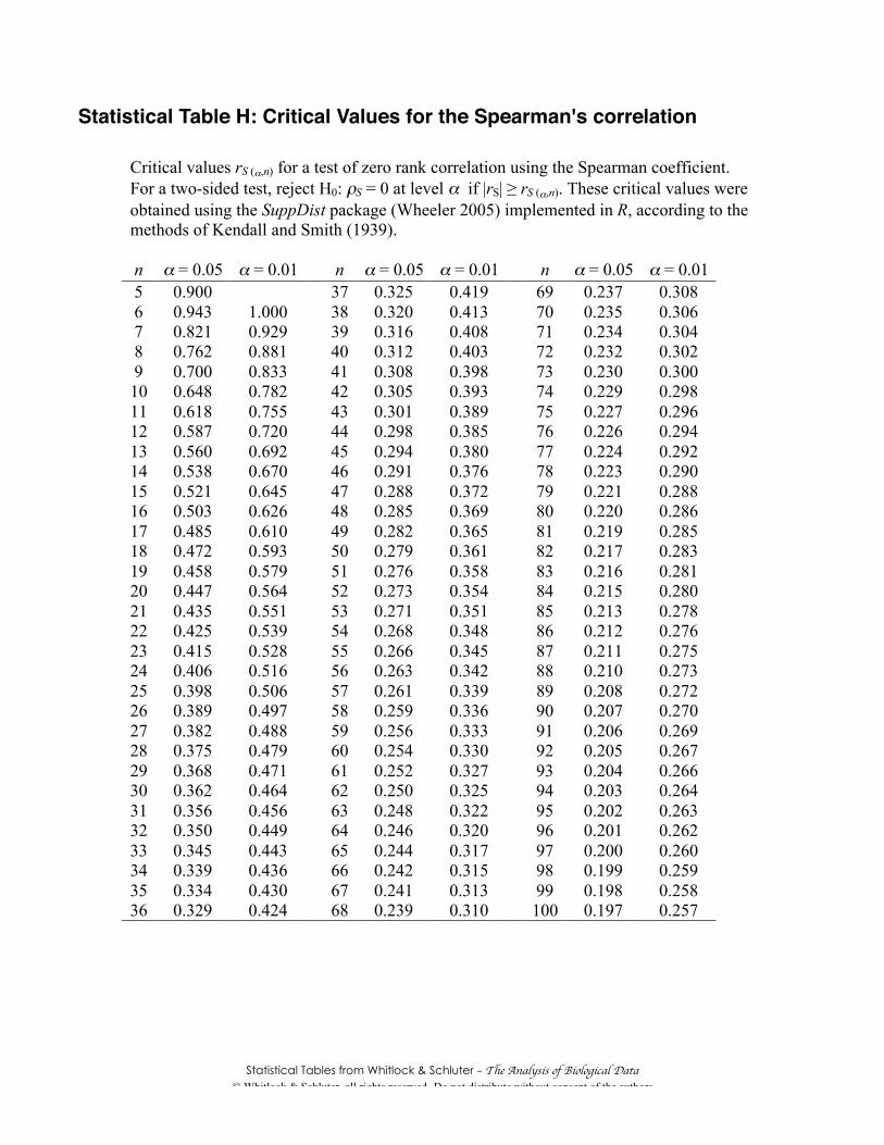
Statistical Table H: Critical Values for the Spearman's correlation

Critical values rS (α,n) for a test of zero rank correlation using the Spearman coefficient.For a two-sided test, reject H0: ρS = 0 at level α if |rS| ≥ rS (α,n). These critical values wereobtained using the SuppDist package (Wheeler 2005) implemented in R, according to themethods of Kendall and Smith (1939).

n α = 0.05 α = 0.01 n α = 0.05 α = 0.01 n α = 0.05 α = 0.015 0.900 37 0.325 0.419 69 0.237 0.3086 0.943 1.000 38 0.320 0.413 70 0.235 0.3067 0.821 0.929 39 0.316 0.408 71 0.234 0.3048 0.762 0.881 40 0.312 0.403 72 0.232 0.3029 0.700 0.833 41 0.308 0.398 73 0.230 0.30010 0.648 0.782 42 0.305 0.393 74 0.229 0.29811 0.618 0.755 43 0.301 0.389 75 0.227 0.29612 0.587 0.720 44 0.298 0.385 76 0.226 0.29413 0.560 0.692 45 0.294 0.380 77 0.224 0.29214 0.538 0.670 46 0.291 0.376 78 0.223 0.29015 0.521 0.645 47 0.288 0.372 79 0.221 0.28816 0.503 0.626 48 0.285 0.369 80 0.220 0.28617 0.485 0.610 49 0.282 0.365 81 0.219 0.28518 0.472 0.593 50 0.279 0.361 82 0.217 0.28319 0.458 0.579 51 0.276 0.358 83 0.216 0.28120 0.447 0.564 52 0.273 0.354 84 0.215 0.28021 0.435 0.551 53 0.271 0.351 85 0.213 0.27822 0.425 0.539 54 0.268 0.348 86 0.212 0.27623 0.415 0.528 55 0.266 0.345 87 0.211 0.27524 0.406 0.516 56 0.263 0.342 88 0.210 0.27325 0.398 0.506 57 0.261 0.339 89 0.208 0.27226 0.389 0.497 58 0.259 0.336 90 0.207 0.27027 0.382 0.488 59 0.256 0.333 91 0.206 0.26928 0.375 0.479 60 0.254 0.330 92 0.205 0.26729 0.368 0.471 61 0.252 0.327 93 0.204 0.26630 0.362 0.464 62 0.250 0.325 94 0.203 0.26431 0.356 0.456 63 0.248 0.322 95 0.202 0.26332 0.350 0.449 64 0.246 0.320 96 0.201 0.26233 0.345 0.443 65 0.244 0.317 97 0.200 0.26034 0.339 0.436 66 0.242 0.315 98 0.199 0.25935 0.334 0.430 67 0.241 0.313 99 0.198 0.25836 0.329 0.424 68 0.239 0.310 100 0.197 0.257

Spearman's sign rank correlation 25


Reference for Spearman's tables:

Wheeler, B. 2005. The SuppDists package, version 1.0-13, April 7, 2005. Gnu PublicLicense version 2.http://cran.r-project.org/src/contrib/Descriptions/SuppDists.html

Kendall, M. and B. B. Smith. 1939. The problem of m rankings. Annals of Mathematical

Statistics 10: 275−287.

Statistical Tables - Department of Zoology, UBCbio300/StatTables.pdf · Statistical Tables from...

Documents

Transcript of Statistical Tables - Department of Zoology, UBCbio300/StatTables.pdf · Statistical Tables from...