
STATISTICAL SIGNAL PROCESSING - IIT Kanpurhome.iitk.ac.in/~kundu/doafinal-2-rev-1.pdf · ·...
21
STATISTICAL SIGNAL PROCESSING Abstract. Statistical signal processing is an important area of research with extensive applications in the fields of communication theory, array processing, seismology, and medical diagnosis. The goal of signal process- ing is to recover characteristics of the underlying process from observed data. The random nature of the signals underscores the need for statis- tical techniques in model formulation, estimation and data analysis. A brief discussion of the different models that have been widely studied in the statistical signal processing literature is provided. In addition, differ- ent methods of estimation are presented, and some unique characteristics of these models are highlighted. Keywords and Phrases. Array model, detection, estimation, multiple sinusoids. AMS Subject Classification. Primary: 62J02, 60F05, 62H12 Signal processing <stat00170> refers to a collection of techniques used to analyze and extract characteristics of signals from physical observations. The signal gener- ated by a mechanical, electrical, or biological system contains information about the underlying system. The signal is usually observed with error caused by electrical, mechanical, thermal interference, or recording error. With the random<stat00825> nature of the signal, statistical techniques play a vital role in signal processing. Statis- tics is used in the formulation of appropriate models to describe the behavior of the system, the development of appropriate techniques for estimation of the model pa- rameters, and the assessment of model performance. Statistical Signal Processing refers to the analysis of signals using appropriate statistical techniques. 1
Transcript of STATISTICAL SIGNAL PROCESSING - IIT Kanpurhome.iitk.ac.in/~kundu/doafinal-2-rev-1.pdf · ·...
STATISTICAL SIGNAL PROCESSING
Abstract. Statistical signal processing is an important area of research
with extensive applications in the fields of communication theory, array
processing, seismology, and medical diagnosis. The goal of signal process-
ing is to recover characteristics of the underlying process from observed
data. The random nature of the signals underscores the need for statis-
tical techniques in model formulation, estimation and data analysis. A
brief discussion of the different models that have been widely studied in
the statistical signal processing literature is provided. In addition, differ-
ent methods of estimation are presented, and some unique characteristics
of these models are highlighted.
Keywords and Phrases. Array model, detection, estimation, multiple sinusoids.
AMS Subject Classification. Primary: 62J02, 60F05, 62H12
Signal processing <stat00170> refers to a collection of techniques used to analyze
and extract characteristics of signals from physical observations. The signal gener-
ated by a mechanical, electrical, or biological system contains information about the
underlying system. The signal is usually observed with error caused by electrical,
mechanical, thermal interference, or recording error. With the random<stat00825>
nature of the signal, statistical techniques play a vital role in signal processing. Statis-
tics is used in the formulation of appropriate models to describe the behavior of the
system, the development of appropriate techniques for estimation of the model pa-
rameters, and the assessment of model performance. Statistical Signal Processing
refers to the analysis of signals using appropriate statistical techniques.
1
The traditional applications of signal processing have been in the areas of spec-
tral estimation<stat0535>, seismology, communications theory, and radar/ sonar
processing. With the rapid growth in technology over the past decades, signal pro-
cessing techniques are now commonly applied in medical diagnosis, climate modeling,
and pattern recognition<stat06503>. For example, doctors measure the electri-
cal activity of the brain using electroencephalograms (EEG). Analysis of EEG data
allows for the detection of key characteristics of the signal including the dominating
frequency called the ‘rhythm’ and pulse activities called ‘spikes’. This analysis en-
ables doctors to diagnose patients with possible abnormalities. In recent years, voice
recognition software has been widely used by financial institutions. Speech processing
involves characterization of the speech waveform from sampled data by estimating its
key amplitudes and frequencies. Pattern recognition is another area of research falling
under the umbrella of statistical signal processing. Applications include analysis of
MRI and PET data to detect tumors in patients, fingerprint analysis and analysis of
data from Geographical Information Systems. In recent years, these techniques have
also been applied to detect and distinguish underground nuclear explosions from nat-
ural seismic activity.
While signal processing has been an important area of research in electrical engi-
neering, the role of statistics is of more recent origin. Over the past few decades, sta-
tistical tools have been widely used in the signal processing literature. These include
time series analysis, Fourier analysis, multivariate techniques, large sample theory,
and nonlinear regression<stat07552>. In many applications however, standard
omnibus techniques are inefficient, and specific algorithms need to be developed. In
addition, as models become more complex, the availability of powerful computers ne-
cessitates the development of faster, more efficient techniques to process and analyze
large data sets. There is a need for collaborative research between engineers and
2
statisticians to address these important problems.
Three different models that have been extensively used and studied in the signal
processing literature will now be discussed. Properties of these models and different
estimation techniques will be described in some detail.
The Multiple Sinusoids Model
In time series, stationary processes are often analyzed in either the time or fre-
quency domain. Spectral estimation has frequently been used in signal processing as
a preliminary tool to extract periodicities in the data, and requires limited knowl-
edge about the underlying model. However, in several applications, the signal may
be modeled as a sum of sinusoidal terms. For these models, determination of the
amplitudes, frequencies, and phases of the component signals is a problem that may
be addressed using statistical methodology. For example, in speech processing, the
pressure waveform recorded may be modeled as a sum of exponentials (see Pinson
[21]). An important problem is to accurately estimate the resonant frequencies of the
vocal tract.
The multiple sinusoids model may be expressed as
y(t) =M∑k=1
αkejωkt + n(t); t = 1, . . . , N. (1)
Here αk’s represent the complex amplitudes of the signals, ωk’s represent the real ra-
dian frequencies of the signals, n(t)’s are complex valued error random variables with
mean zero and finite variance, and j =√−1. The assumption of independence of the
error random variables is not critical to the development of inferential procedures. The
problem of interest is to estimate the unknown parameters {(αk, ωk); k = 1, . . . ,M}
given a sample of size N . In several applications, the number of signals, M , may also
be unknown. In this case, we first obtain an estimate of M , and then proceed with
the estimation of the amplitudes and frequencies. For a detailed description of the
3
model and applications, one may refer to Kay [10] and Rao [22].
Classical techniques such as the periodogram may be used to estimate the signal
frequencies. The periodogram estimator provides an optimal solution in the case of
single or multiple sinusoids that are well resolved by Fourier methods. However, in
most practical situations it is not possible to resolve the frequencies, and alternative
methods of estimation need to be considered.
The multiple sinusoids model may be considered as a standard nonlinear regres-
sion model with additive error. Therefore, the method of least squares<stat03205>
may be used to estimate the regression parameters. The least squares estimators are
known to have optimal large sample properties such as consistency<stat05836> and
asymptotic normality<stat02818>. If the error term is assumed to be Gaussian
<stat01043>, these are also the maximum likelihood estimators <stat02663>.
The least squares estimators of the unknown parameters can be obtained by mini-
mizing
Q(α,ω) =N∑t=1
∣∣∣∣∣y(t)−M∑k=1
αkejωkt
∣∣∣∣∣2
(2)
with respect to the unknown parameters α = (α1, . . . , αM) and ω = (ω1, . . . , ωM).
Though the multiple sinusoid model falls into the class of nonlinear regression
models, it does not satisfy the sufficient conditions required for the consistency of the
least squares estimators. In fact, the model does not satisfy the crucial assumption
of identifiability<stat06411>. Therefore, it is important to determine whether or
not the method of least squares is appropriate for this problem. A second problem is
to develop iterative techniques to obtain the least squares estimates.
The violation of standard assumptions is a problem frequently encountered in sig-
nal processing models. These features certainly provide a challenge from a statistical
and technical point of view, and require creative solutions. In particular, nonstan-
dard techniques are needed to obtain large sample properties of the estimators. For
4
the multiple sinusoids model, the periodic nature of the sinusoidal components have
been exploited to prove the consistency and asymptotic normality of the least squares
estimators.
For the nonlinear regression model under standard regularity conditions, the least
squares estimators are known to be consistent with asymptotic variance of order
N−1. For the multiple sinusoids model, the least squares estimators of the linear
parameters αk’s are consistent with asymptotic variance of order N−1. The least
squares estimators of the nonlinear parameters are consistent, however, with the rate
of convergence of order N−32 . One may refer to Kundu and Mitra [12] for further
technical details.
The least squares estimators may be obtained by solving M linear and M non-
linear equations. Since the nonlinear surface Q(α,ω) is not well behaved, the choice
of the initial value is critical, and standard algorithms suffer from convergence to
local minima. Several iterative techniques have been developed based on Prony’s
difference equations and the idea of separable regression. These iterative techniques
are computationally intensive, but are numerically more stable.
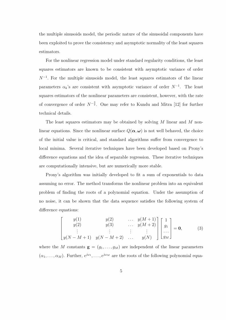
Prony’s algorithm was initially developed to fit a sum of exponentials to data
assuming no error. The method transforms the nonlinear problem into an equivalent
problem of finding the roots of a polynomial equation. Under the assumption of
no noise, it can be shown that the data sequence satisfies the following system of
difference equations:y(1) y(2) . . . y(M + 1)y(2) y(3) . . . y(M + 2)
......
......
y(N −M + 1) y(N −M + 2) . . . y(N)
1g1. . .gM
= 0, (3)
where the M constants g = (g1, . . . , gM) are independent of the linear parameters
(α1, . . . , αM). Further, ejω1 , . . . , ejωM are the roots of the following polynomial equa-
5
tion:
1 + g1z + . . .+ gMzM = 0. (4)
Prony’s algorithm thus provides a 1-1 correspondence between {g1, . . . , gM} and
{ω1, . . . , ωM}.
The first step in Prony’s algorithm is to determine the coefficients of the polyno-
mial by solving the linear system in (3). The roots of this polynomial provide the
frequencies, and subsequently, the estimates of the linear parameters are obtained
using ordinary least squares. The coefficients of the polynomial may be obtained
through quadratic optimization, solving a nonlinear eigenvalue problem, or the ex-
pectation maximization (EM) algorithm<stat00410>. A review of these and
other comparable procedures can be found in Bresler and Macovski [4], Kannan and
Kundu [9] and Kundu and Nandi [13].
The iterative algorithms developed for obtaining the least squares estimates are
numerically challenging and time consuming. They are clearly not suited for adaptive
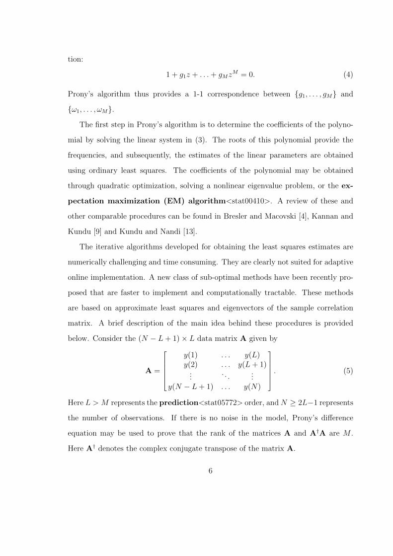
online implementation. A new class of sub-optimal methods have been recently pro-
posed that are faster to implement and computationally tractable. These methods
are based on approximate least squares and eigenvectors of the sample correlation
matrix. A brief description of the main idea behind these procedures is provided
below. Consider the (N − L+ 1)× L data matrix A given by
A =
y(1) . . . y(L)y(2) . . . y(L+ 1)
.... . .
...y(N − L+ 1) . . . y(N)
. (5)
Here L > M represents the prediction<stat05772> order, and N ≥ 2L−1 represents
the number of observations. If there is no noise in the model, Prony’s difference
equation may be used to prove that the rank of the matrices A and A†A are M .
Here A† denotes the complex conjugate transpose of the matrix A.
6
The null space of the matrix A†A contains information on the signal frequencies.
In the presence of noise, the matrix is of full rank L > M , and may be approximated
by a matrix of lower rank M using the singular value decomposition. The eigenvectors
corresponding to the zero eigenvalue may be used to recover the frequencies. Tufts
and Kumaresan [27] have examined the performance of these estimators for different
L. The problem of choosing the optimal prediction order L has been considered by
several other authors, but a satisfactory solution has not yet been found.
Another interesting approach to estimate the frequencies of the model (1) is known
as the iterative filtering method. The basic idea of the iterative filtering method is
that
E(y(t)) = µ(t) =M∑k=1
αkejωkt, for t = 1, . . . , N,
satisfies a homogeneous autoregressive (AR) equation of order 2M . Then based on the
observations, the estimation of the corresponding AR parameters are performed using
parametric filtering method. Since there is a one to one correspondence between the
AR parameters and the frequencies of the model (1), once the AR parameters are es-
timated, the estimation of the frequencies can be obtained quite easily. Li and Kadem
[15] first proposed this method, then Song and Li [25] provided some biased corrected
version of the iterative filtering method. Li and Song [16] provided an estimation pro-
cedure of the frequencies when the errors follow Laplace distribution<stat01040>,
and Kundu et al. [11] provided a super efficient estimation procedure of the frequen-
cies which converges faster than the usual least squares estimators. For some recent
references and for a review of the different existing methods, see Peng et al. [19] and
Kundu and Nandi [13].
Remark 1. A closely related model in time series assumes real valued signals. The
7
model may be expressed as
y(t) =p∑
k=1
Ak cos(ωkt+ φk) + ε(t), (6)
where Ak’s are real valued amplitudes, ωk’s are the frequencies, and φk’s are the phase
components. The error random variables ε(t) are real valued with mean zero and
finite variance. The independence assumption simplifies the estimation procedures;
however, dependence structures may be easily incorporated. All the methods of
estimation that have been presented for model (1) may be adapted for this model.
Multidimensional Sinusoids Model
The high resolution performance of frequency estimators for the multiple sinu-
soids model has prompted recent interest in the multidimensional problem. The two
dimensional version of model (1) plays an important role in image processing, sonar
and seismic data analysis, and in texture classification. An extensive development
of two-dimensional and multidimensional digital signal processing may be found in
Dudgeon and Mersereau [5]. A two-dimensional version of model (1) can be described
as follows:
y(s, t) =M∑k=1
αkej(λks+µkt) + n(s, t); s = 1, . . . , S, t = 1, . . . , T. (7)
Here αk’s are complex valued amplitudes, λk’s and µk’s are unknown frequencies. The
error random variables n(s, t) are assumed to have mean zero and finite variance. The
problem once again involves estimation of the signal parameters αk’s, λk’s and µk’s
from data {y(s, t)}.
Some of the estimation procedures available for the one-dimensional problem may
be extended easily to two dimensions. However, several technical difficulties arise
when dealing with high dimensional data. There are several open problems in multi-
dimensional frequency estimation, and this continues to be an active area of research.
8
Recently, Bian et al. [2] proposed an efficient estimation method for two dimensional
frequency model. For some of the recent references interested readers are refereed to
Peng et al. [18] and the references cited therein.
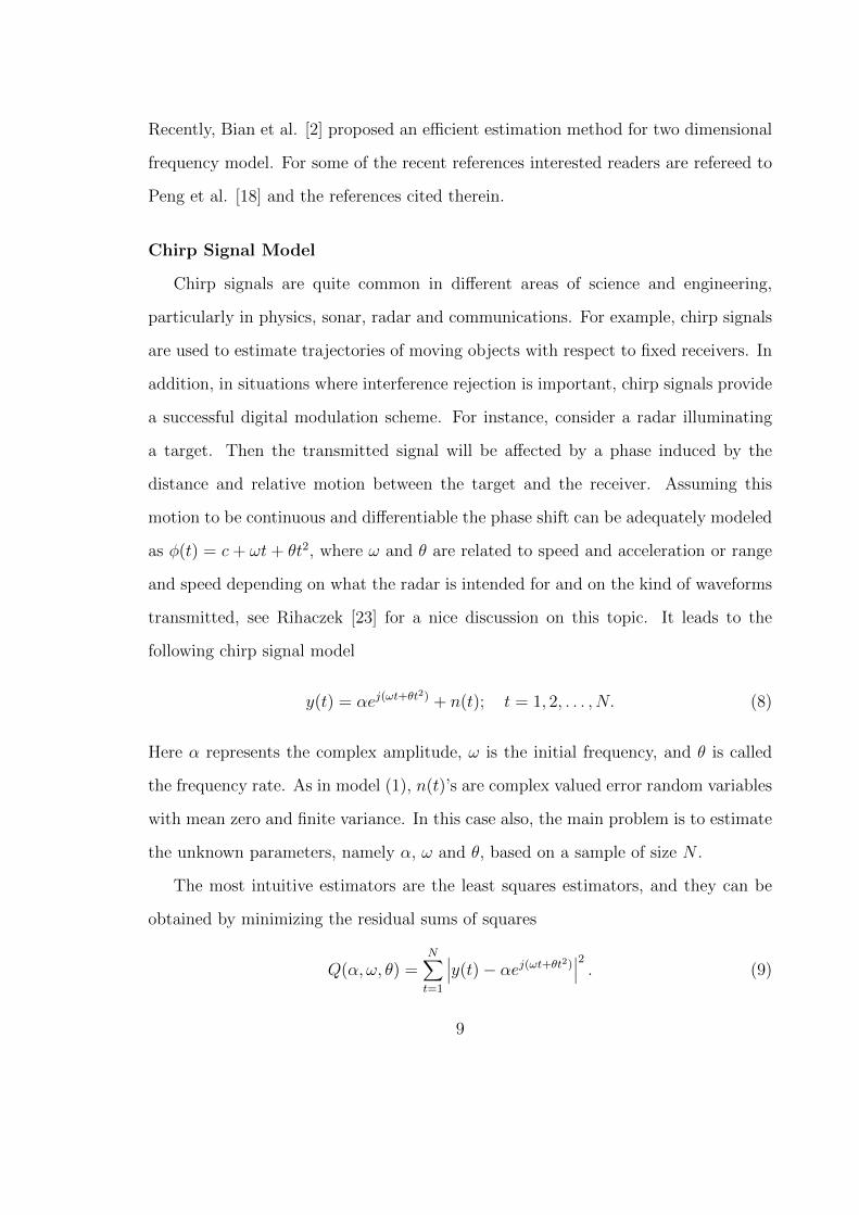
Chirp Signal Model
Chirp signals are quite common in different areas of science and engineering,
particularly in physics, sonar, radar and communications. For example, chirp signals
are used to estimate trajectories of moving objects with respect to fixed receivers. In
addition, in situations where interference rejection is important, chirp signals provide
a successful digital modulation scheme. For instance, consider a radar illuminating
a target. Then the transmitted signal will be affected by a phase induced by the
distance and relative motion between the target and the receiver. Assuming this
motion to be continuous and differentiable the phase shift can be adequately modeled
as φ(t) = c+ ωt+ θt2, where ω and θ are related to speed and acceleration or range
and speed depending on what the radar is intended for and on the kind of waveforms
transmitted, see Rihaczek [23] for a nice discussion on this topic. It leads to the
following chirp signal model
y(t) = αej(ωt+θt2) + n(t); t = 1, 2, . . . , N. (8)
Here α represents the complex amplitude, ω is the initial frequency, and θ is called
the frequency rate. As in model (1), n(t)’s are complex valued error random variables
with mean zero and finite variance. In this case also, the main problem is to estimate
the unknown parameters, namely α, ω and θ, based on a sample of size N .
The most intuitive estimators are the least squares estimators, and they can be
obtained by minimizing the residual sums of squares
Q(α, ω, θ) =N∑t=1
∣∣∣y(t)− αej(ωt+θt2)∣∣∣2 . (9)
9
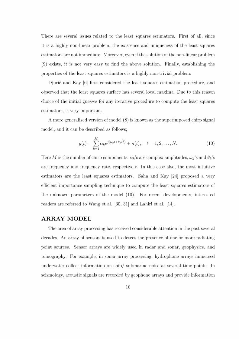
There are several issues related to the least squares estimators. First of all, since
it is a highly non-linear problem, the existence and uniqueness of the least squares
estimators are not immediate. Moreover, even if the solution of the non-linear problem
(9) exists, it is not very easy to find the above solution. Finally, establishing the
properties of the least squares estimators is a highly non-trivial problem.
Djuric and Kay [6] first considered the least squares estimation procedure, and
observed that the least squares surface has several local maxima. Due to this reason
choice of the initial guesses for any iterative procedure to compute the least squares
estimators, is very important.
A more generalized version of model (8) is known as the superimposed chirp signal
model, and it can be described as follows;
y(t) =M∑k=1
αkej(ωkt+θkt
2) + n(t); t = 1, 2, . . . , N. (10)
Here M is the number of chirp components, αk’s are complex amplitudes, ωk’s and θk’s
are frequency and frequency rate, respectively. In this case also, the most intuitive
estimators are the least squares estimators. Saha and Kay [24] proposed a very
efficient importance sampling technique to compute the least squares estimators of
the unknown parameters of the model (10). For recent developments, interested
readers are referred to Wang et al. [30, 31] and Lahiri et al. [14].
ARRAY MODEL
The area of array processing has received considerable attention in the past several
decades. An array of sensors is used to detect the presence of one or more radiating
point sources. Sensor arrays are widely used in radar and sonar, geophysics, and
tomography. For example, in sonar array processing, hydrophone arrays immersed
underwater collect information on ship/ submarine noise at several time points. In
seismology, acoustic signals are recorded by geophone arrays and provide information
10
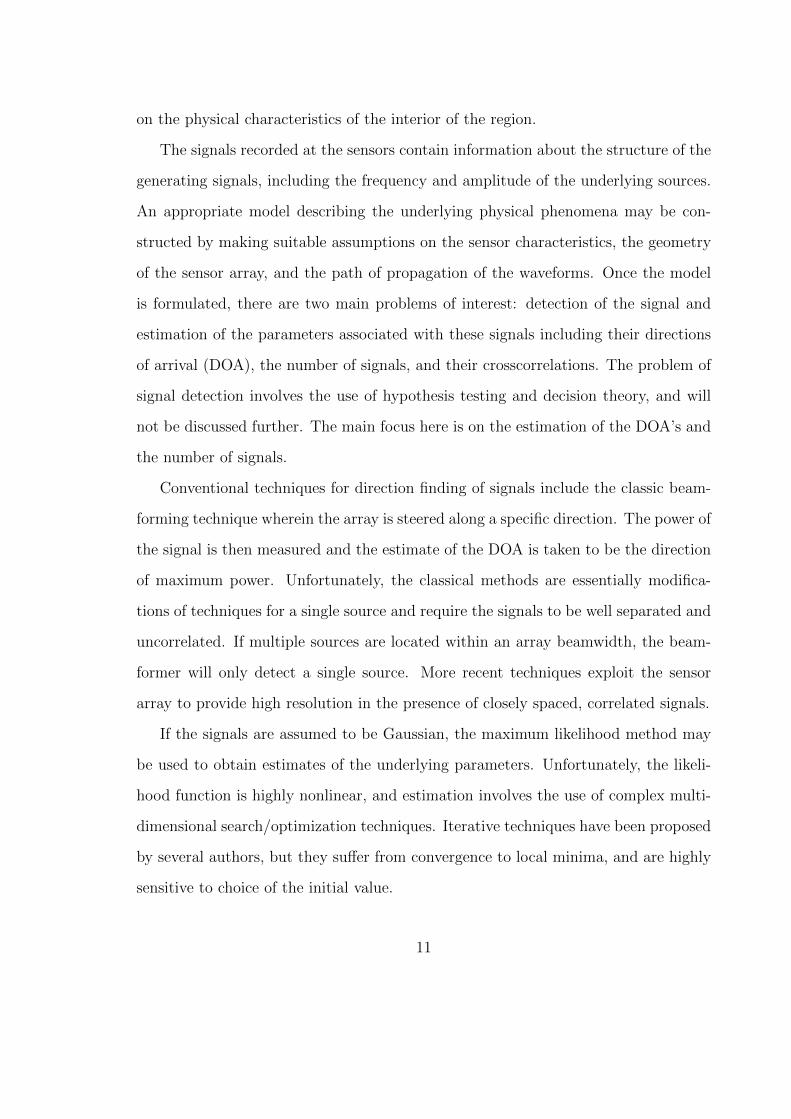
on the physical characteristics of the interior of the region.
The signals recorded at the sensors contain information about the structure of the
generating signals, including the frequency and amplitude of the underlying sources.
An appropriate model describing the underlying physical phenomena may be con-
structed by making suitable assumptions on the sensor characteristics, the geometry
of the sensor array, and the path of propagation of the waveforms. Once the model
is formulated, there are two main problems of interest: detection of the signal and
estimation of the parameters associated with these signals including their directions
of arrival (DOA), the number of signals, and their crosscorrelations. The problem of
signal detection involves the use of hypothesis testing and decision theory, and will
not be discussed further. The main focus here is on the estimation of the DOA’s and
the number of signals.
Conventional techniques for direction finding of signals include the classic beam-
forming technique wherein the array is steered along a specific direction. The power of
the signal is then measured and the estimate of the DOA is taken to be the direction
of maximum power. Unfortunately, the classical methods are essentially modifica-
tions of techniques for a single source and require the signals to be well separated and
uncorrelated. If multiple sources are located within an array beamwidth, the beam-
former will only detect a single source. More recent techniques exploit the sensor
array to provide high resolution in the presence of closely spaced, correlated signals.
If the signals are assumed to be Gaussian, the maximum likelihood method may
be used to obtain estimates of the underlying parameters. Unfortunately, the likeli-
hood function is highly nonlinear, and estimation involves the use of complex multi-
dimensional search/optimization techniques. Iterative techniques have been proposed
by several authors, but they suffer from convergence to local minima, and are highly
sensitive to choice of the initial value.
11
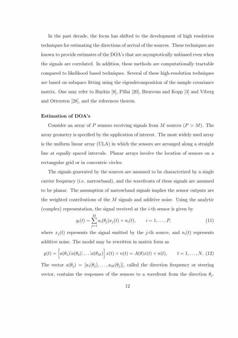
In the past decade, the focus has shifted to the development of high resolution
techniques for estimating the directions of arrival of the sources. These techniques are
known to provide estimates of the DOA’s that are asymptotically unbiased even when
the signals are correlated. In addition, these methods are computationally tractable
compared to likelihood based techniques. Several of these high-resolution techniques
are based on subspace fitting using the eigendecomposition of the sample covariance
matrix. One may refer to Haykin [8], Pillai [20], Bienvenu and Kopp [3] and Viberg
and Ottersten [28], and the references therein.
Estimation of DOA’s
Consider an array of P sensors receiving signals from M sources (P > M). The
array geometry is specified by the application of interest. The most widely used array
is the uniform linear array (ULA) in which the sensors are arranged along a straight
line at equally spaced intervals. Planar arrays involve the location of sensors on a
rectangular grid or in concentric circles.
The signals generated by the sources are assumed to be characterized by a single
carrier frequency (i.e. narrowband), and the wavefronts of these signals are assumed
to be planar. The assumption of narrowband signals implies the sensor outputs are
the weighted contributions of the M signals and additive noise. Using the analytic
(complex) representation, the signal received at the i-th sensor is given by
yi(t) =M∑j=1
ai(θj)xj(t) + ni(t), i = 1, . . . , P, (11)
where xj(t) represents the signal emitted by the j-th source, and ni(t) represents
additive noise. The model may be rewritten in matrix form as
y(t) =[a(θ1)
...a(θ2)... . . .
...a(θM)]x(t) + n(t) = A(θ)x(t) + n(t), t = 1, . . . , N. (12)
The vector a(θj) = [a1(θj), . . . , aM(θj)], called the direction frequency or steering
vector, contains the responses of the sensors to a wavefront from the direction θj.
12
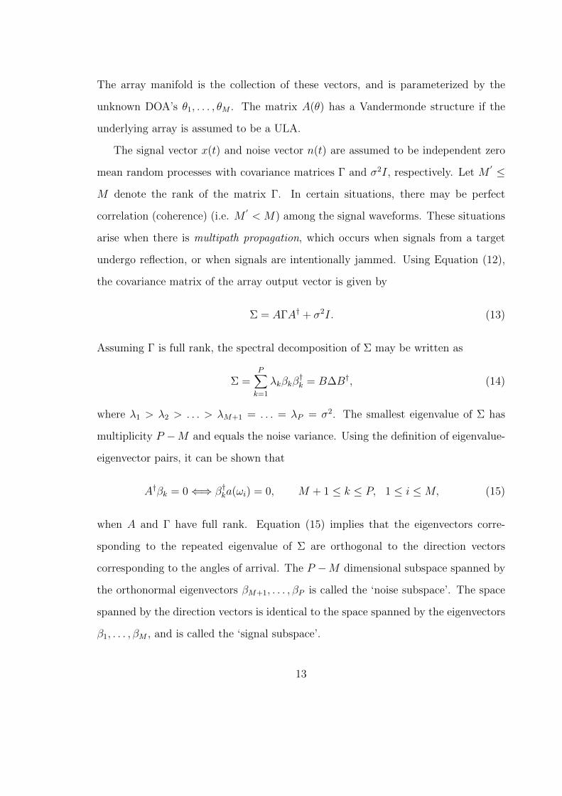
The array manifold is the collection of these vectors, and is parameterized by the
unknown DOA’s θ1, . . . , θM . The matrix A(θ) has a Vandermonde structure if the
underlying array is assumed to be a ULA.
The signal vector x(t) and noise vector n(t) are assumed to be independent zero
mean random processes with covariance matrices Γ and σ2I, respectively. Let M′ ≤
M denote the rank of the matrix Γ. In certain situations, there may be perfect
correlation (coherence) (i.e. M′< M) among the signal waveforms. These situations
arise when there is multipath propagation, which occurs when signals from a target
undergo reflection, or when signals are intentionally jammed. Using Equation (12),
the covariance matrix of the array output vector is given by
Σ = AΓA† + σ2I. (13)
Assuming Γ is full rank, the spectral decomposition of Σ may be written as
Σ =P∑k=1
λkβkβ†k = B∆B†, (14)
where λ1 > λ2 > . . . > λM+1 = . . . = λP = σ2. The smallest eigenvalue of Σ has
multiplicity P −M and equals the noise variance. Using the definition of eigenvalue-
eigenvector pairs, it can be shown that
A†βk = 0⇐⇒ β†ka(ωi) = 0, M + 1 ≤ k ≤ P, 1 ≤ i ≤M, (15)
when A and Γ have full rank. Equation (15) implies that the eigenvectors corre-
sponding to the repeated eigenvalue of Σ are orthogonal to the direction vectors
corresponding to the angles of arrival. The P −M dimensional subspace spanned by
the orthonormal eigenvectors βM+1, . . . , βP is called the ‘noise subspace’. The space
spanned by the direction vectors is identical to the space spanned by the eigenvectors
β1, . . . , βM , and is called the ‘signal subspace’.
13
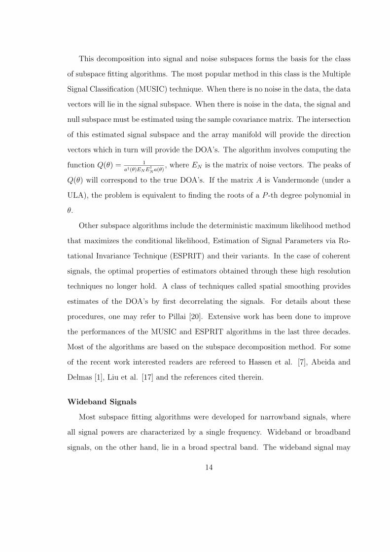
This decomposition into signal and noise subspaces forms the basis for the class
of subspace fitting algorithms. The most popular method in this class is the Multiple
Signal Classification (MUSIC) technique. When there is no noise in the data, the data
vectors will lie in the signal subspace. When there is noise in the data, the signal and
null subspace must be estimated using the sample covariance matrix. The intersection
of this estimated signal subspace and the array manifold will provide the direction
vectors which in turn will provide the DOA’s. The algorithm involves computing the
function Q(θ) = 1
a†(θ)ENE†Na(θ)
, where EN is the matrix of noise vectors. The peaks of
Q(θ) will correspond to the true DOA’s. If the matrix A is Vandermonde (under a
ULA), the problem is equivalent to finding the roots of a P -th degree polynomial in
θ.
Other subspace algorithms include the deterministic maximum likelihood method
that maximizes the conditional likelihood, Estimation of Signal Parameters via Ro-
tational Invariance Technique (ESPRIT) and their variants. In the case of coherent
signals, the optimal properties of estimators obtained through these high resolution
techniques no longer hold. A class of techniques called spatial smoothing provides
estimates of the DOA’s by first decorrelating the signals. For details about these
procedures, one may refer to Pillai [20]. Extensive work has been done to improve
the performances of the MUSIC and ESPRIT algorithms in the last three decades.
Most of the algorithms are based on the subspace decomposition method. For some
of the recent work interested readers are refereed to Hassen et al. [7], Abeida and
Delmas [1], Liu et al. [17] and the references cited therein.
Wideband Signals
Most subspace fitting algorithms were developed for narrowband signals, where
all signal powers are characterized by a single frequency. Wideband or broadband
signals, on the other hand, lie in a broad spectral band. The wideband signal may
14
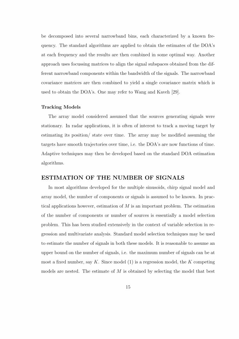
be decomposed into several narrowband bins, each characterized by a known fre-
quency. The standard algorithms are applied to obtain the estimates of the DOA’s
at each frequency and the results are then combined in some optimal way. Another
approach uses focussing matrices to align the signal subspaces obtained from the dif-
ferent narrowband components within the bandwidth of the signals. The narrowband
covariance matrices are then combined to yield a single covariance matrix which is
used to obtain the DOA’s. One may refer to Wang and Kaveh [29].
Tracking Models
The array model considered assumed that the sources generating signals were
stationary. In radar applications, it is often of interest to track a moving target by
estimating its position/ state over time. The array may be modified assuming the
targets have smooth trajectories over time, i.e. the DOA’s are now functions of time.
Adaptive techniques may then be developed based on the standard DOA estimation
algorithms.
ESTIMATION OF THE NUMBER OF SIGNALS
In most algorithms developed for the multiple sinusoids, chirp signal model and
array model, the number of components or signals is assumed to be known. In prac-
tical applications however, estimation of M is an important problem. The estimation
of the number of components or number of sources is essentially a model selection
problem. This has been studied extensively in the context of variable selection in re-
gression and multivariate analysis. Standard model selection techniques may be used
to estimate the number of signals in both these models. It is reasonable to assume an
upper bound on the number of signals, i.e. the maximum number of signals can be at
most a fixed number, say K. Since model (1) is a regression model, the K competing
models are nested. The estimate of M is obtained by selecting the model that best
15
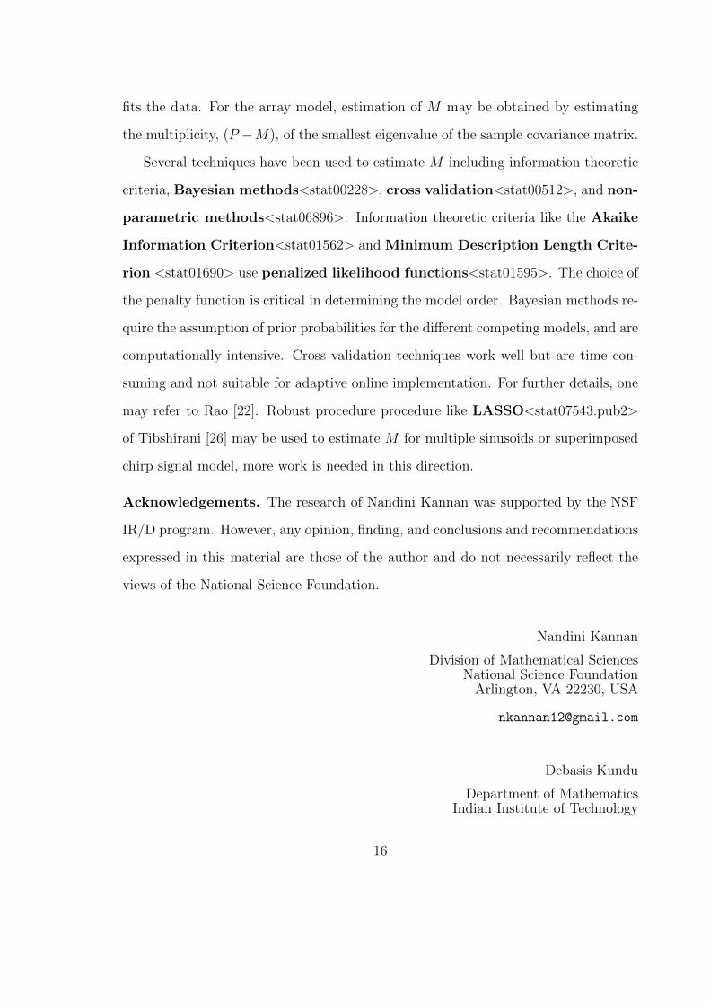
fits the data. For the array model, estimation of M may be obtained by estimating
the multiplicity, (P −M), of the smallest eigenvalue of the sample covariance matrix.
Several techniques have been used to estimate M including information theoretic
criteria, Bayesian methods<stat00228>, cross validation<stat00512>, and non-
parametric methods<stat06896>. Information theoretic criteria like the Akaike
Information Criterion<stat01562> and Minimum Description Length Crite-
rion <stat01690> use penalized likelihood functions<stat01595>. The choice of
the penalty function is critical in determining the model order. Bayesian methods re-
quire the assumption of prior probabilities for the different competing models, and are
computationally intensive. Cross validation techniques work well but are time con-
suming and not suitable for adaptive online implementation. For further details, one
may refer to Rao [22]. Robust procedure procedure like LASSO<stat07543.pub2>
of Tibshirani [26] may be used to estimate M for multiple sinusoids or superimposed
chirp signal model, more work is needed in this direction.
Acknowledgements. The research of Nandini Kannan was supported by the NSF
IR/D program. However, any opinion, finding, and conclusions and recommendations
expressed in this material are those of the author and do not necessarily reflect the
views of the National Science Foundation.
Nandini Kannan
Division of Mathematical SciencesNational Science Foundation
Arlington, VA 22230, USA
Debasis Kundu
Department of MathematicsIndian Institute of Technology
16
Kanpur, 208016, INDIA
References
[1] Abeida, H. and Delmas, J-P. (2008). Statistical performance of MUSIC-like algo-
rithms in resolving noncircular sources, IEEE Transactions on Signal Processing,
56, 4317 - 4329.
[2] Bian, J., Li, H., Peng, H. (2011). An efficient and fast algorithm for estimating the
frequencies of 2-D superimposed exponential signals in zero-mean multiplicative
and additive noise, Journal of Statistical Planning and Inference, 141, 1277 -
1289.
[3] Bienvenu, G. and Kopp, L. (1980). Adaptivity to Background Noise Spatial
Coherence for High Resolution Passive Methods, Proceedings of the IEEE Inter-
national Conference on Acoustics, Speech and Signal Processing, 307–310.
[4] Bresler, Y. and Macovski, A. (1986). Exact Maximum Likelihood Parameter
Estimation of Superimposed Exponential Signals in Noise, IEEE Transactions
on Acoustics, Speech, and Signal Processing, 34, 1081-1089.
[5] Dudgeon, D.E. and Mersereau, R.M. (1984). Multidimensional Digital Signal
Processing, Prentice-Hall, Englewood Cliffs, New Jersey.
[6] Djuric, P.M. and Kay, S.M. (1990). Parameter estimation of chirp signals, IEEE
Transactions on Acoustics Speech and Signal Processing, 38, 2128 - 2126.
17
[7] Hassen, S.B., Bellili, F., Samet, A. and Affes, S. (2011). DOA estimation of
temporally and spatially correlated narrowband noncircular sources in spatially
correlated white noise, IEEE Transactions on Signal Processing, 59, 4108 - 4121.
[8] Haykin, S. (1985). Array Signal Processing, Prentice-Hall, Englewood Cliffs, New
Jersey.
[9] Kannan, N. and Kundu, D. (1994). On Modified EVLP and ML Methods of
Estimating Superimposed Exponential Signals, Signal Processing, 39, 223-233.
[10] Kay, S.M. (1987). Modern Spectral Estimation, Prentice Hall, New York, NY.
[11] Kundu, D., Bai, Z.D., Nandi, S. and Bai, L. (2011). Super efficient frequency
estimation, Journal of Statistical Planning and Inference, 141, 2576 - 2588.
[12] Kundu, D. and Mitra, A. (1999). On Asymptotic Behavior of Least Squares
Estimators and the Confidence Intervals of the Superimposed Exponential, Signal
Processing, 72, 129-139.
[13] Kundu, D. and Nandi, S. (2012). Statistical signal processing: frequency estima-
tion, Springer, New Delhi.
[14] Lahiri, A., Kundu, D. and Mitra, A. (2015). Estimating the parameters of mul-
tiple chirp signals, Journal of Multivariate Analysis, 139, 189 – 206.
[15] Li, T-H and Kadem, B. (1996). Itertaive filtering for multiple frequency estima-
tion, IEEE Transactions on Signal Processing, 42, 1120 - 1132.
[16] Li, T-H. and Song, K-S. (2009). Estimation of the parameters of sinusoidal signals
in non-Gaussian noise, IEEE Transactions on Signal Processing, 57, 62-72.
18
[17] Liu, Z-M., Huang, Z-T., Zhou, Y-Y. Liu, J. (2012). Direction-of-arrival esti-
mation of noncircular signals via sparse representation, IEEE Transactions on
Aerospace and Electronic Systems, 48, 2690 - 2698.
[18] Peng, H., Bian, J., Yang, D., Liu, Z., Li, H. (2014). Statistical analysis of param-
eter estimation for 2-D harmonics in multiplicative and additive noise Journal
of Applied Statistics, 43, DOI:10.1080/03610926.2012.746985.
[19] Peng, H., Yu, S., Bian, J., Zhang, Y., Li, H. (2015). Statistical analysis of non
linear least squares estimation for harmonic signals in multiplicative and additive
noise, Communication in Statistics- Theory and Methods, 44, 217 - 240.
[20] Pillai, S. U. (1989). Array Signal Processing, Springer-Verlag, New York, NY.
[21] Pinson, E.N. (1963). Pitch-synchronous Time-domain Estimation of Formant
Frequencies and Bandwidth, Journal of Acoustics Society of America, 35, 1264-
1273.
[22] Rao, C.R. (1988). Some Recent Results in Signal Detection, In Statistical Deci-
sion Theory and Related Topics, IV (Eds. Gupta, S.S. and Berger, J.O.), Vol. 2,
319-332, Springer-Verlag, New York, NY.
[23] Rihaczek, A.W. (1969). Principles of High Resolution Radar, McGraw Hill, New
York.
[24] Saha, S. and Kay, S.M. (2002). Maximum likelihood parameter estimation of su-
perimposed chirps using Monte Carlo importance sampling, IEEE Transactions
on Signal Processing, 50, 224 - 230.
19
[25] Song, K-S and Li, T-H. (2006). On coevergence and bias correction of a joint es-
timation algorithm for multiple sinusoidal frequencies”, Journal of the American
Statistical Association, 101, 830 - 842.
[26] Tibshirani, R. (1996). Regression shrinkage and selection via the Lasso, Journal
of the Royal Statistical Society, Ser. B. 267 – 288.
[27] Tufts, D.W. and Kumaresan, R. (1982). Estimation of Frequencies of Multiple
Sinusoids: Making Linear Prediction Perform Like Maximum Likelihood, Pro-
ceedings of the IEEE, 70, 975-989.
[28] Viberg, M. and Ottersten, B. (1991). Sensor Array Processing Based on Subspace
Fitting, IEEE Transactions on Signal Processing, 39, 1110-1121.
[29] Wang, H. and Kaveh, M. (1985). Coherent Signal Subspace Processing for the
Detection and Estimation of Angles of Arrival of Multiple Wide-band Sources,
IEEE Transactions on Acoustics, Speech, and Signal Processing, 33, 823–831.
[30] Wang, P., Djurovic, I.and Yang, J. (2008). Generalized high-order phase func-
tion for parameter estimation of polynomial phase signal, IEEE Transactions on
Signal Processing, 56, 3023 – 3028, 2008.
[31] Wang, P., Li, P., Djurovic, and Himed, B. (2010). Performance of instantaneous
frequency rate estimation using high-order phase function, IEEE Transactions
on Signal Processing, 58, 2415 – 2421.
Further Reading
Bose, N.K. and Rao, C.R. (1993). Signal Processing and its Applications, Handbook
of Statistics, Vol. 10, North-Holland, Amsterdam.
20
Srinath, M.D., Rajasekaran, P.K. and Viswanathan, R. (1996), Introduction to Sta-
tistical Signal Processing with Applications, Prentice-Hall, Englewood Cliffs, New
Jersey.
Quinn, B.G. and Hannan, E.J. (2001), The estimation and tracking of frequency,
Cambridge University Press, New York.
Related Entries:
stat03220
stat03281
stat04554
stat03519
stat03517
LATEXtemplate, Wiley
21


![[Monson H. Hayes] Statistical Digital Signal Processing](https://static.fdocuments.in/doc/165x107/563db7e3550346aa9a8ee680/monson-h-hayes-statistical-digital-signal-processing.jpg)


![[Steven M. Kay] Fundamentals of Statistical Signal](https://static.fdocuments.in/doc/165x107/55cf8ef2550346703b9748fc/steven-m-kay-fundamentals-of-statistical-signal.jpg)