Statistical Shape Analysis Ian Dryden (University of ...gerig/CS7960-S2010/handouts/... ·...
49
Statistical Shape Analysis Ian Dryden (University of Nottingham) [email protected] http://www.maths.nott.ac.uk/ ild 3e cycle romand de statistique et probabilit ´ es appliqu ´ es Les Diablerets, Switzerland, March 7-10, 2004. 1 Session I Dryden and Mardia (1998, chapters 1,2,3,4) Introduction Motivation and applications Size and shape coordinates Shape space Shape distances. 2 In a wide variety of applications we wish to study the geometrical properties of objects. We wish to measure, describe and compare the size and shapes of objects Shape: location, rotation and scale information (simi- larity transformations) can be removed. [Kendall, 1984] Size-and-shape: location, rotation (rigid body trans- formations) can be removed. 3 An object’s shape is invariant under the similarity trans- formations of translation, scaling and rotation. Two mouse second thoracic vertebra (T2 bone) out- lines with the same shape. 4
Transcript of Statistical Shape Analysis Ian Dryden (University of ...gerig/CS7960-S2010/handouts/... ·...

Statistical Shape Analysis
Ian Dryden (University of Nottingham)
http://www.maths.nott.ac.uk/ � ild
3e cycle romand de statistique et probabilitesappliques
Les Diablerets, Switzerland, March 7-10, 2004.
1
Session I
Dryden and Mardia (1998, chapters 1,2,3,4)� Introduction� Motivation and applications� Size and shape coordinates� Shape space� Shape distances.
2
In a wide variety of applications we wish to study thegeometrical properties of objects.
We wish to measure, describe and compare the sizeand shapes of objects
Shape: location, rotation and scale information (simi-larity transformations) can be removed. [Kendall, 1984]
Size-and-shape: location, rotation (rigid body trans-formations) can be removed.
3
An object’s shape is invariant under the similarity trans-formations of translation, scaling and rotation.
Two mouse second thoracic vertebra (T2 bone) out-lines with the same shape.
4
Guido Gerig
Typewritten Text
http://www.stat.sc.edu/~dryden/course/ild-ch-04.pdf

From Galileo (1638) illustrating the differences in shapesof the bones of small and large animals.
5
� Landmark: point of correspondence on each objectthat matches between and within populations.
Different types: anatomical (biological), mathematical,pseudo, quasi
6
T2 mouse vertebra with six mathematical landmarks(line junctions) and 54 pseudo-landmarks.
7
� Bookstein (1991)
Type I landmarks (joins of tissues/bones)Type II landmarks (local properties such as maximalcurvatures)Type III landmarks (extremal points or constructed land-marks)
� Labelled or un-labelled configurations
8

F
1 2
3
A
1
2
3
B
2
1
3
D
2
1
3
2C
1
3
E
2
3
1
Six labelled triangles: A, B have the same size andshape; C has the same shape as A, B (but larger size);D has a different shape but its labels can be permutedto give the same shape as A, B, C; triangle E can bereflected to have the same shape as D; triangle F hasa different shape from A,B,C,D,E.
9
Traditional methods
- ratios of distances between landmarks or angles sub-mitted to multivariate analysis
- the full geometry usually if often lost
- collinear points?
- interpretation of shape differences in multivariate space?
10
Geometrical shape analysis
Rather than working with quantities derived from or-ganisms one works with the complete geometrical ob-ject itself (up to similarity transformations).
In the spirit of D’Arcy Thompson (1917) who consid-ered the geometric transformations of one species toanother
We conside a shape space obtained directly from thelandmark coordinates, which retains the geometry ofa point configuration at all stages.
11
� Pioneers: Fred Bookstein and David Kendall
Summaries of the field are given by Bookstein (1991,Cambridge), Small (1996, Springer), Dryden and Mar-dia (1998, Wiley), Kendall et al (1999, Wiley), Lele andRichstmeier (2001, Chapman and Hall).
12

MR brain scan
13
The map of 52 megalithic sites (+) that form the ‘OldStones of Land’s End’ in Cornwall (from Stoyan et al.,1995).
14
-0.4 -0.2 0.0 0.2 0.4
-0.4
-0.2
0.0
0.2
0.4
1 2 3
4
56
7 89
10
11
1213
Handwritten digit 3
15
pr
ba o
l
b
n
na
st
Face
Braincase
Ape cranium
16
(a) (b)
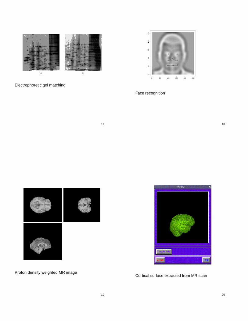
Electrophoretic gel matching
17
0 50 100 150 200 250
050
100
150
200� 25
0
S S
S S
SS S
SS
• •
• •
•
• •
••
Face recognition
18
Proton density weighted MR image
19
Cortical surface extracted from MR scan
20

203 Pseudo-landmarks on the cortical surface of thebrain
21
OUR FOCUS:�
landmarks in � real dimensions�is a
� � � matrix ( � � � � � � � � � � � � � � � � � �)
Invariance with respect to Euclidean similarity group(translation, scale and rotation) = � � � � � � � � � � �Size....
Any positive real valued function � � � � such that � � � � � �� � � � � for a positive scalar�.
22
� Centroid size:
� � � � � � � � � ! �"# $ % �"& $ % � � # & ' (� & � )where (� & � %� * �# $ % � # & and
� + � ' ,� , � , - �� � � � ! � . / � � � � - � � - Euclidean norm,+ � -
� � �identity matrix, , � -
� � , vector of ones.
23
An alternative size measure is the baseline size, i.e.the length between landmarks 1 and 2:
0 % ) � � � � � � � � ) ' � � � % � 1This was used as early as 1907 by Galton for normal-izing faces.
Other size measures: square root of area, cube rootof volume
24

Shape coordinates:
Fixed coordinate system
vs
Local Coordinate system
Are angles appropriate.....??
1
2
3
12
3
12 3
25
Landmarks: 2 % 3 2 ) 3 1 1 1 3 2 � 4 5� Bookstein shape coordinates (1984,1986) (For twodimensional data)
••
••
•
•
•
Re(z)
Im(z
)
-200 -100 0 100 200
-200
-100
010
020
06•
•
••
•
•
•
Re(z)
Im(z
)
-200 -100 0 100 200
-200
-100
010
020
06•
•
•
•
••
•
Re(z)
Im(z
)
-200 -100 0 100 200
-200
-100
010
020
0
•
•
•
•
•
•
•
Re(z)
Im(z
)
-0.5 0.0 0.5
-0.5
0.0
0.5
1.0
Shape: 7 8& � 9 : ; 9 <9 = ; 9 < ' > 1 ? 3 � @ � A 3 1 1 1 3 � �26
••
•
•
(a)
-20 -10 0 10 20
-20
-10
010
20
12
3
••
•
•
(b)
-20 -10 0 10 20
-20
-10
010
20
12
3
• •
•
•
(c)
-20 -10 0 10 20
-20
-10
010
20
1 2
3
• •
•
•
(d)
-0.5 0.0 0.5
-0.5
0.0
0.5
1.0
1 2
3
In real co-ordinates:B CD $ ; %) � E F 9 G ; 9 H I F 9 D ; 9 H I � F J G ; J H I F J D ; J H I K L M G H G NO CD $ E F 9 G ; 9 H I F J D ; J H I ; F J G ; J H I F 9 D ; 9 H I K L M G H G Nwhere
& $ P N Q Q Q N �, M G H G $ F 9 G ; 9 H I G � F J G ; J H I G R S and; T U B CD N O CD U T .
27
The outline of a microfossil with three landmarks (fromBookstein, 1986).
28

•
•
•
•
•
•
•
••
•
•
•
•
•
•••
•
•
•
•
U
V
V0.2 0.3 0.4 0.5 0.6
0.4
0.5
0.6
0.7
0.8
60
65
64
65
67
71
72
7174
75
76
84
84
84
878888
88
92
100
100
A scatter plot of (U+1/2) for the Bookstein shape vari-ables for some microfossil data. (Bookstein, 1986)
29
slog
0.32W
0.36 0.40 0.44
•
• •••
• ••• ••
•• •••••
•
• •
8.2
8.4
8.6
8.8
9.0X 9.
2
•
• • ••
•• •• ••
•• ••• •
•
• •
0.32Y 0.
360.
400.
44
•
•
•
•
• •
•
•
•••
••• •
•
•
••
•
•
U
•
•
•
•
• •
•
•
•••
••
• ••
•
••
•
•
8.2 8.4 8.6 8.8 9.0 9.2•
•
•
•
•
••
• •
••
•
•
••••
••
•
•
•
•
•
•
••
••
••
•
•
••••
•
••
•
0.45W
0.55 0.65 0.75W 0.
450.
550.
650.
75
V
30
uZ
v
-0.5 0.0[
0.5[-0
.50.
00.
5
1\
2]
6^
3_
5` 4
a
A scatter plot of the Bookstein shape variables for theT2 mouse data.
31
Bb
Uc
VB
-2 -1 0[
1\
2]-2
-10
12
EdF
eAf
Bb
Og
The shape space of triangles, using Bookstein’s co-ordinates
� h 8 3 i 8 � . All triangles could be relabelledand reflected to lie in the shaded region.
32

Kendall’s shape coordinates
Remove location j k � l j m � � j % 3 1 1 1 3 j � ; % � -7 n& o p q n& � j & ; %j % � @ � A 3 1 1 1 3 � � 1
Simple 1-1 linear correspondence with Booklstein S.V.(equ. 2.11 of book)
For triangles Kendall’s SV sends baseline to ' , r ! A 3 , r ! A33
� Kendall’s shape sphere (1983) (triangles only)
Flat triangles
1 2
3
1 2
3
Isosceles triangles Equilateral (North pole)
Reflected equilateral (South pole)
(Equator)
Right-angled Unlabelled
φ=0 φ=π/3
φ=5π/3 φ=2π/3θ=π/2
θ=0
θ=π
A mapping from Kendall’s shape variables to the sphereis
2 � , ' s )t � , o s ) � 3 u � 7 nP, o s ) 3 j � q nP, o s )and s ) � � 7 nP � ) o � q nP � ) , so that2 ) o u ) o j ) � %v .
34
Kendall’s spherical shape shape variables� w 3 x � are
then given by the usual polar coordinates
2 � ,t � � � w � � � x 3 u � ,t � � � w � � � x 3 j � ,t � � � w 3where > y w y z is the angle of latitude and > y x {t z is the angle of longitude.
35
Kendall’s Bell
36
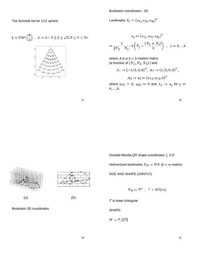
The Schmidt net for 1/12 sphere
| � t � � � } wt ~ 3 � � x � > y | y ! t 3 > y � { t z 1
-0.5 0.0 0.5
-1.5
-1.0
-0.5
0.0
•A BC
•A BC
•A BC
•A BC •A B
C •A BC
•A BC
•A BC
•A BC •A B
C •A BC •A B
C
•A BC
•A BC•A BC •A BC •A B
C•A BC
•A BC
•A BC•A BC •A BC
•A BC•A BC
•A BC
•A BC•A BC •A BC
•A BC
•A BC
•A B
C
•A B
C•
A B
C
•A BC
•A BC
•A BC •A B
C
37
Bookstein coordinates - 3D
Landmarks� # � � 2 % # 3 2 ) # 3 2 P # � -
7 & � � 7 % & 3 7 ) & 3 7 P & � -� ,� � ) ' � % � � � � & ' � � % o � ) �t � 3 @ � A 3 1 1 3 �where � is a A � A rotation matrix(a function of
� � % 3 � ) 3 � P � ) and� % � � ' , r t 3 > 3 > � - 3 � ) � � , r t 3 > 3 > � - 3� P � 7 P � � 7 % P 3 7 ) P 3 > � -where 7 ) P � > , 7 P P � > and
� & � 7 & for@ �� 3 1 1 1 3 �
.
38
(a) (b)
Bookstein 3D coordinates
39
Goodall-Mardia QR shape coordinates � tD
Helmertized landmarks� k � l �
(� � � matrix)
SIZE AND SHAPE (JOINTLY)
� k � � � 3 � 4 � � � � � 3� is lower triangular
SHAPE:� � � r � � �40

Shape coordinates
1. FILTER OUT TRANSLATION:
a) Shift centroid to originb) Take linear orthogonal contrasts, e.g. Helmert con-trastsc) Shift baseline midpoint to origin
2. RE-SCALE:
a) Re-scale to unit centroid sizeb) Re-scale to unit areac) Re-scale to a standard baseline lengthd) Re-scale to minimize ‘distance’ to a template
3. REMOVE ROTATION:
a) Rotate baseline to horizontalb) Rotate to minimize ‘distance’ to a template
Bookstein shape coordinates: 1c/2c/3aKendall shape coordinates: 1b/2c/3aProcrustes shape coordinates: 1a/2d/3b
41
SHAPE SPACE....Kendall (1984)
1. Remove location (Pre-multiply by Helmert sub-matrix)� k � l �where
@th row of the Helmert sub-matrix l is given
by,� � & 3 1 1 1 3 � & 3 ' @ � & 3 > 3 1 1 1 3 > � 3 � & � ' � @ � @ o , � � ; <=and the
� & is repeated@
times and zero is repeated� ' @ ' , times,@ � , 3 1 1 1 3 � ' , .
Note � l - l (centering matrix) so � � � � � � � k � �� � � � 1 (centroid size)
42
2. Remove size (rescale)� � � k� � � � � l �� l � � 1� �
is the PRESHAPE ( 4 � F � ; % I � ; %)
3. Remove rotation� � � � � � � � � 4 � � � � � � 3� � � �is the SHAPE of
�.
43
� Dimensions....
Original configuration:� � �
Centered configuration:� � ' �
Preshape:� � ' � ' ,
Shape:� � ' � ' , ' � � � ' , � r t
� Shape space is non-Euclidean
44

SHAPE SPACES
Assume� � � o , . [
�points in � Euclidean dimen-
sions]� � , : � � % is a unit radius� � ' t � -sphere.� � t
: � �) is the complex projective space 5 � � ; ) .� � t: � �� has a singularity set z � � � ; ) � of dimen-
sion � ' tand is NOT a homogeneous space.
For � � tthe space spaces � � � %� are topological
spheres.
45
Write � $ � � � N S � � , for the pseudo-singular value decom-position where
� � � � F � ; % I N � � � � F � ; % I , and� $� � � F ¡ H N Q Q Q N ¡ ¢ I . Let£ ¤¢ $ ¥ E � � � ¤¢ ¦ ¡ H R Q Q Q R ¡ ¢ § H R ¨ ¡ ¢ ¨ K � © � $ � � %E � � � ¤¢ ¦ ¡ H R Q Q Q R ¡ ¢ § H R ¡ ¢ K � © � R � � %
Le and DG Kendall (1993, Annals of Statistics)
Theorem On ª F £ ¤¢ I , the Riemannian metric can be expressedas « ¬ G $ ¢" ® G « ¡ G � � ¢" ® G ¡ ¡ H « ¡ � G � "H ¯ ° D ¯ ¢ F ¡ G ; ¡ GD I G¡ G � ¡ GD ± G D
� ¢" ® H ¤ § H"D ® ¢ ² H ¡ G ± G D Nwhere ± D are co-ordinates for
� � F � ; % I .
46
Planar case: � � tdimensional data� �� � � �) r � � � t � � 5 � � ; )
Helmertized landmarksj k � l j m � � j % 3 1 1 1 3 j � ; % � - 4 5 � ; % � > �Now multiplying by³ � s � # ´ 3 � s 4 � 3 µ 4 � > 3 t z � �rotates and rescales j k . So,
� ³ j k � ³ 4 5 � > � � 3is the set representing the SHAPE of j m . This is acomplex line through the origin (but not including it) in� ' , dimensions. The union of all such sets is thecomplex projective space 5 � � ; )NB: 5 � � ; ) ¶ � )
47
PLANAR CASE: Procrustes/Riemannian distance
Complex configurations j m � � j m % 3 1 1 1 3 j m� � - 3· m � � · m % 3 1 1 1 3 · m� � -with centroids j ¸ 3 · ¸ .
Shape distance ¹ � j m 3 · m � satisfies
� � � ¹ � j m 3 · m � � º * �# $ % � j m# ' j ¸ � � · m# ' · ¸ � º! * � j m# ' j ¸ � ) ! * � · m# ' · ¸ � )where · m# means the complex conjugate of · m# .
NB� � � ¹ is the modulus of the complex correlation
between j m and · m .� � � A : ¹ is the great circle distance on� ) � , r t � .
48

Complex configurations j m � � j m % 3 1 1 1 3 j m� � -Bookstein co-ordinates:· 8& � j m& ' j m %j m) ' j m % ' > 1 ? 3 � @ � A 3 1 1 1 3 � �Kendall co-ordinates:· n& � j & ; % r j & 3 � @ � A 3 1 1 1 3 � �where
� j % 3 1 1 1 3 j � ; % � - � l j m� Linear relationship:» n � ! t l % » 8where l % is lower right
� � ' t � � � � ' t � partition ofl .
For� � A : · 8P � � ! A r t � · nP .
49
Session II� Procrustes analysis� Tangent coordinates� Shape variability� Shape models� Tangent space inference� Shapes package.
50
PROCRUSTES ANALYSIS
Juvenile (———) Adult (- - - - - -)
••
•
•
•
•
••
••••
x
y
-2000 -1000 0 1000 2000 3000
-200
0-1
000
010
0020
0030
00
•
•
•
•
••
•
••
••
•
•
••
•
•
•
•
••
••••
x
y
-2000 -1000 0 1000 2000 3000
-200
0-1
000
010
0020
0030
00
••
•
•
•
•
••••••
•
Register adult onto juvenile
51
PLANAR PROCRUSTES ANALYSIS
Two centred configurations u � � u % 3 1 1 1 3 u � � ¼ and· � � · % 3 1 1 1 3 · � � ¼ , both in 5 �, withu ½ , � � > � · ½ , � ,
[ u ½ - transpose of the complex conjugate of u ]
Match · onto u using complex linear regression
u � � � o p ¾ � , � o ¿ � # À · o Á� � , � 3 · � � o Á� � M � o Á 3� M � � , � 3 · �- ‘design’ matrix� � � � o p ¾ 3 ¿ � # À � ¼ - similarity transformation pa-
rameters
52

Procrustes match = least squares
Minimize the sum of square errors0 ) � u 3 · � � Á ½ Á � � u ' � M � � ½ � u ' � M � � 1Full Procrustes fit (superimposition) of · on u
·  � � M Ã� � � Ã� o p à ¾ � , � o ÿ � # ÄÀ · 3where
Ã� � � � ½M � M � ; % � ½M u ,i.e. Ã� o p à ¾ � > 3Ãw � / . Å � · ½ u � � ' / . Å � u ½ · � 3ÿ � � · ½ u u ½ · � % L ) r � · ½ · � 1
53
Procrustes fit · Â � · ½ u · r � · ½ · �Procrustes residual vector s � u ' · ÂMinimized objective function0 ) � s 3 > � � u ½ u ' � u ½ · · ½ u � r � · ½ · �(not symmetric unless u ½ u � · ½ · )
Initially standardize to unit centroid size....
Full Procrustes distance:Æ Ç � · 3 u � � � � ÈÉ N À N Ê N Ë ÌÌÌÌÌu� u � ' ·� · � ¿ � # À ' � ' p ¾ ÌÌÌÌÌ� Í , ' u ½ · · ½ u· ½ · u ½ u Î % L ) 1
54
FULL Procrustes distanceÆ Ç
- full set of similaritytransformations used in matching
PARTIAL Procrustes distanceÆ Â - matching over trans-
lation and rotation ONLY
For fairly similar shapes they are very similar,as
Æ Ç � Æ Â o � � Æ PÂ � � ¹ o � � ¹ P �In this course for simplicity we shall concentrate onFULL Procrustes matching.
55
1 1
ρ
ρ/2
F
/2P
d
d
Section of the pre-shape sphere
56

1/2 1/2
ρ
dF
d/2ρ
Section of the SHAPE SPHERE FOR TRIANGLES,illustrating the relationship between
Æ Ç,
Æ Â and ¹57
Procrustes residuals from the match of · onto u aredifferent from u onto ·
•
•
•
•
••
•
••
••
•
x
y
-2000 -1000 0 1000 2000 3000
-200
0-1
000
010
0020
0030
00
••
•
•
••
•
••
••
•
JUV to ADULT (above): Ãw � � ? 1 ? Ï , ÿ � , 1 , A , .ADULT to JUV: Ãw Ð � ' � ? 1 ? Ï , ÿ Ð � > 1 Ñ Ò ? Ó�, r , 1 , A ,
58
Female (left) and Male (right) gorilla skulls
x
(a)
y
-300 -200 -100 0 100
-100
010
020
0
x
(b)
y
-300 -200 -100 0 100
-100
010
020
0
Mean shape? Shape variance/covariance?
59
CONFIGURATION MODEL
Random sample of Ô configurations · % 3 1 1 1 3 · Õ fromthe perturbation model· # � Ö # , � o ¿ # � # À × � Ø o Á # � 3 p � , 3 1 1 1 3 Ô 3where Ö # 4 5 - translations¿ # 4 � - scales> y w # { t z - rotationsÁ # 4 5 are independent zero mean complex randomerrorsØ
is the population mean configuration.
AIM: to estimate
� Ø �- the shape of
ØProcrustes mean:� ÃØ � � / . Å � � ÈÙ Õ"# $ % Æ )Ç � · # 3 Ø � 1
60

Consider · # to be centred: · -# , � � > .
(Kent,1994)Procrustes mean shape
� ÃØ �is the dom-
inant eigenvector of� � Õ"# $ % · # · ½# r � · ½# · # � � Õ"# $ % j # j ½# 3where the j # � · # r � · # � 3 p � , 3 1 1 1 3 Ô , are the pre-shapes.
Proof We wish to minimizeÕ"# $ % Æ )Ç � · # 3 Ø � � Õ"# $ % Í , ' Ø ½ · # · ½# Ø· ½# · # Ø ½ Ø Î� Ô ' Ø ½ � Ø r � Ø ½ Ø � 1Therefore, ÃØ � / . Å � Ú ÛÜ Ù Ü $ % Ø ½ � Ø 1Hence, result follows.
61
� Procrustes fits: match · # to ÃØ· Â# � · ½# ÃØ · # r � · ½# · # � 3 p � , 3 1 1 1 3 Ô 3
NB Arithmetic mean:%Õ * Õ# $ % · Â# has same shape asÃØ
.� Procrustes residuals
s # � · Â# ' ÝÞ ,Ô Õ"# $ % · Â# ßà 3 p � , 3 1 1 1 3 Ô 362
Procrustes fits (Generalized Procrustes analysis)
• •
••
•
•
• •
-0.6 -0.4 -0.2 0.0 0.2 0.4 0.6
-0.6
-0.4
-0.2
0.0
0.2
0.4
0.6
• •
••
•
•
• •
• •
••
•
•
• •
• •
••
•
•
• •
• •
•••
•
• •
••
••
•
•
• •
• •
••
•
•
••
••
••
•
•
• •
• •
••
•
•
• •
••
••
•
•
••
• •
••
•
•
••
• •
••
•
•
• •
• •
••
•
•
• •
• •
••
•
•
••
• •
••
•
•
• •
• •
••
•
•
• •
• •
••
•
•
• •
• •
••
•
•
• •
• •
••
•
•
• •
• •
••
•
•
• •
• •
••
•
•
• •
• •
••
•
•
• •
• •
••
•
•
••
• •
••
•
•
••
• •
••
•
•
• •
• •
••
•
•
••
• •
••
•
•
• •
• •
••
•
•
• •
• •
••
•
•
• •
• •
••
•
•
• •
• •
••
•
•
• •
Female gorillas
63
••
•••
•
••
-0.6 -0.4 -0.2 0.0 0.2 0.4 0.6
-0.6
-0.4
-0.2
0.0
0.2
0.4
0.6
••
•••
•
••
• •
•••
•
• •
• •
••
•
•
••
• •
•••
•
• •
• •
•••
•
• •
• •
••
•
•
• •
• •
•••
•
••
• •
•••
•
• •
• •
••
•
•
••
• •
•••
•
• •
• •
•••
•
••
• •
•••
•
••
• •
•••
•
• •
• •
•••
•
••
• •
••
•
•
• •
• •
••
•
•
• •
• •
•••
•
• •
• •
••
•
•
••
• •
•••
•
• •
••
•••
•
••
• •
••
•
•
••
• •
•••
•
• •
• •
•••
•
• •
• •
••
•
•
• •
• •
••
•
•
• •
• •
••
•
•
• •
• •
•••
•
• •
• •
••
•
•
• •
• •
•••
•
• •
Male Gorillas

x
y
-150 -100 -50 0 50 100 150
-150
-100
-50
050
100
150
The male (—-) and female (- - -) full Procrustes meanshapes registered by GPA.
64
Other mean shape estimates:� Bookstein mean shape
Take sample mean of Bookstein coordinatesh 8
• •
•
•
•
•
•
•
u
vá-1.0 -0.5 0.0 0.5 1.0
-1.0
-0.5
0.0
0.5
1.0
7 4
1
2
3
5
6
8â
1
2
3
5
6
8â
1
2ã
3ä
5å
6
8
1
2ã
3
5å
6
8â
1
2
3
5å
6
8
1
2
3ä
5
6
8â
1
2
3
5
6
8
1
2ã
3
5
6
8
1
2ã
3
5
6
8â
1
2ã
3
5å
6
8
1
2ã
3
5
6
8
1
2
3
5
6
8
1
2
3ä
5
6
8
1
2ã
3ä
5å
6
8
1
2
3
5
6
8
1
2
3
5
6
8
1
2
3
5
6
8
1
2
3ä
5
6
8
1
2
3
5
6
8â
1
2
3
5
6
8
1
2
3
5
6
8
1
2ã
3ä
5
6
8
1
2
3
5å
6
8
1
2
3
5
6
8
1
2
3
5
6
8
1
2
3
5
6
8
1
2
3
5å
6
8
1
2
3
5
6
8â
1
2ã
3
5
6
8
1
2
3
5
6
8â
Female Gorillas
65
• •
•
•
•
•
•
•
u
v
-1.0 -0.5 0.0 0.5 1.0
-1.0
-0.5
0.0
0.5
1.0
7 4
1
2
3
5
6
8
1
2
3
5
6
8
1
2
3
5
6
8
1
2
3
5
6
8
1
2
3
5
6
8
1
2
3
5
6
8
1
2
3
5
6
8
1
2
3
5
6
8
1
2
3
5
6
8
1
2
3
5
6
8
1
2
3
5
6
8
1
2
3
5
6
8
1
2
3
5
6
8
1
2
3
5
6
8
1
2
3
5
6
8
1
2
3
5
6
8
1
2
3
5
6
8
1
2
3
5
6
8
1
2
3
5
6
8
1
2
3
5
6
8
1
2
3
5
6
8
1
2
3
5
6
8
1
2
3
5
6
8
1
2
3
5
6
8
1
2
3
5
6
8
1
2
3
5
6
8
1
2
3
5
6
8
1
2
3
5
6
8
1
2
3
5
6
8
Male Gorillas
66
[In Book chapter 12]� MDS mean shape (Kent, 1994; Lele 1991)
Obtain average squared Euclidean distance matrix0
let æ � ' %) 0 (centred inner product matrix)
Let ç % 3 1 1 1 3 ç è be the scaled eigenvectors� 0 � � � 0 � � � ç % 3 ç ) 3 1 1 1 3 ç � �(invariant under reflections too)� IMPORTANT: If shape variations small the meanshape estimates are approximately linearly related.i.e. Multivariate normal based inference will be equiv-alent to first order. (Kent, 1994)
67

Tangent coordinates
Consider complex landmarks j m � � j m % 3 1 1 1 3 j m� � ¼ withpre-shapej � � j % 3 1 1 1 3 j � ; % � ¼ � l j m r � l j m � 1Let Ö be a complex pole on the complex pre-shapesphere usually chosen as an average shape.
Let us rotate the configuration by an anglew
to be asclose as possible to the pole and then project ontothe tangent plane at Ö , denoted by � � Ö � . Note thatÃw � / . Å � ' Ö ½ j � minimizes � Ö ' j � # À � ) .
68
The partial Procrustes tangent coordinates for aplanar shape are given byq � � # ÄÀ � + � ; % ' Ö Ö ½ � j 3 q 4 � � Ö � 3 (1)
where Ãw � / . Å � ' Ö ½ j � . Partial Procrustes tangentcoordinates involve only rotation (and not scaling) tomatch the pre-shapes.
Note that q ½ Ö � > and so the complex constraintmeans we can regard the tangent space as a realsubspace of ) � ; ) of dimension
t � ' �. The ma-
trix + � ; % ' Ö Ö ½ is the matrix for complex projectioninto the space orthogonal to Ö . Below we see a sec-tion of the shape sphere showing the tangent planecoordinates.
69
PROCRUSTES TANGENT SPACE
Procrustes tangent co-ordinates � of�
at the pole� : � � é � ' � � � ¹ �where > { ¹ y z r t
is the Riemannian distance be-tween the shapes of � and
�, and é is the optimal
Procrustes rotation to match�
to � .
RX
ρcos
T
M
The rays from the origin in Procrustes tangent spacecorrespond to minimal geodesics in shape space.
70
v
γ
zeiθ
zei βθ
Fv
A diagrammatic view of a section of the pre-shapesphere, showing the partial tangent plane coordinatesq and the full Procrustes tangent plane coordinatesq Ç
. Note that the inverse projection from q to j � # ÄÀis
given byj � # ÄÀ � � � , ' q ½ q � % L ) Ö o q � 3 j 4 5 � � ; ) 1 (2)
Hence an icon for partial Procrustes tangent coordi-nates is given by
� ê � l ¼ j .71

+ +
+
+
+
+
-0.6 -0.4 -0.2 0.0 0.2 0.4 0.6
-0.6
-0.4
-0.2
0.0
0.2
0.4
0.6
+ +
+
+
+
+
+ +
+
+
+
+
+ +
+
+
+
+
+ +
+
+
+
+
+ +
+
+
+
+
+ +
+
+
+
+
+ +
+
+
+
+
+ +
+
+
+
+
+ +
+
+
+
+
+ +
+
+
+
+
+ +
+
+
+
+
+ +
+
+
+
+
+ +
+
+
+
+
+ +
+
+
+
+
+ +
+
+
+
+
+ +
+
+
+
+
++
+
+
+
+
+ +
+
+
+
+
+ +
+
+
+
+
++
+
+
+
+
+ +
+
+
+
+
+ +
+
+
+
+
+ +
+
+
+
+
11 2
6
35
4
Icons for partial Procrustes tangent coordinates forthe T2 vertebral data (Small group).
72
s
-0.54-0.48
••• ••
••••
••••
•
••••
•
••
•• •• ••
•
••• •••
••
•
•• • •
•
••
• •
0.07 0.10
••••
•
• •••
•••
••
••••
•
••• • •
••••
•••
•• •
••
•
•• ••
•
••
••
-0.10 -0.06
••••
•
•• ••••
••
•
••••
•
•••• •
•• ••
• •••
• ••
••
••••
•
••••
-0.18 -0.10
•• •••
••••
• ••
••
••• •
•
••
• • •• ••
•
••••
• ••
••
•• ••
•
••••
0.14 0.17
•• ••
•
• •••
•••
••
•• ••
•
••
• • ••• •
•
• • ••
••••
•
••••
•
••
••
0.1450.170ë
••••
•
•• •••••
••
••••
•
••
• •
165
180
•••••
• • ••••
••
•
•• ••
•
••
• •
-0.5
4-0.
48
• •••
•• •••
••
• •
••
•••
•
••
•• x1 •• ••
• ••• •
••
••
••
•• •
•
••
• •••
••
• • •• •
••
••
••
•••
•
••• •
••••
•••• •
••
••
•••
•••
••
••• •••
••• ••
••
• •
•••••
•
••••
• •••
•• •••
••
••
••
••••
••••
•• ••
• ••••
••
••
••
•• •
•
••
• ••• •
•• ••••
••
••
••
•••
•
••••
•• ••
•• •• •
••
• •
••
•••
•
••
• •• ••
••• • ••
••
••
••
•••
•
••
••• ••
•••• ••
••
• •
•••
•••
••
• •• ••
••• • ••
••
• •
•••
•••
••
• •
•
•
••
•••••
••
• •
••
•••
••
•
•• •
•
••
••••• ••
••
••
•••
••
•
•• x2 •
•
••
• ••• •
••
••
••
•••
••
•
•• •
•
••
•••• •
• •
••
••
•••
••
•
•• •
•
••
••• ••
••
• •
••
•••
•••
•• •
•
••
•• •••• •
••
••
••••
••
•• •
•
••
• ••••• •
••
••
•• •
•••
•• •
•
••• ••••• •
••
••
•••
••
•
•• •
•
••
•••• •
••
• •
••
•••
••
•
•• •
•
••
••• ••
••
••
••
•••
••
•
•• •
•
••
••• ••••
• •
••
••••
••
••
0.46
0.52•
•
••
••• ••••
• •
••
•••
•••
••
0.07
0.10
• ••• •
••
••
••
•
• ••
•••
•
•• •• ••• •
•
••
••
••
•
• ••
•••
•
•• •• ••
•••
••
••
••
•
•••
• • •
•
•••
• x3 •••• •
••
••• •
•
•••• ••
•
•• •
• • •••
•
••
••••
•
• •••••
•
•••
• • •• •
•
••
••
• •
•
•••
•••
•
•••• ••
•••
••
••
• •
•
•••
•• •
•
•••
• •••••
••
••
• •
•
•••
• ••
•
•••• ••
•• •
••
••
••
•
•••
• ••
•
•••
• • •• ••
••
••
••
•
• ••
•••
•
•• •
• • •••
•
••
••••
•
••••••
•
•••• • •
•••
••
••••
•
•••• ••
•
••••
• •••
•• •
•• •
•• •
•• •
•••
••
••
••• ••
•••• ••••
•• •••
••
•
••
••••
•••
•••
• ••
•••
• ••
••
••
••••
•• •
•••
• ••
•••
•••
••
•• x4
• •••
•••
••••• •
•••••
•••
••
• •• •
•• •
•••
•••
•• •
•••
••
••
••••
•••
•••• ••
•••
• ••
••
••
•••••
•••••• ••
•••
•••
••
••
••••
•• •
•• ••• •
•••••
••
•
••
• •• ••
• ••
• ••••
•• •
•••
••
••
• •••
•••••••• •
••••••
••
••
-0.0
20.
02• •••
•• •
•••
• • •
•••
•••••
••
-0.1
0-0
.06
•••
•••
•
•
• ••
••
•• ••••
•• •• •
•• ••••
•
• ••
••
•• •••
••• •
• •• •
•• ••
•
•••
••
••• • •
•• ••• •
•••
• ••
•
•••
••
••••• •
•••• •
•••
•••
•
•• •
••
••• ••
•• • •
• x5 •••
••••
•
•• •
••
•• •••
••••
• •• •
•• •
•
•
•• •
••
•••• •
••••
• •• ••• ••
•
•• •
••
••• ••
•• ••
• •• ••
•••
•
• ••
••
••• ••
•• ••
• ••••
•••
•
• ••
••
•• •••
••• •
• •••
•••
•
•
•••
••
••••••• ••• •
•••
•••
•
•••
••
••• ••
•••••
•
•
••
•• ••• •
•• ••
••••••• •• •
•
••
••••• •
••••
••
••••• •• •
•
••
• ••• ••
• •••
••
• • •• •• • •
•
••
• • •• ••
• •••
•••• •
••• • •
•
••
•••• ••
••••
••
•••• • •• •
•
••
••• •••
•• ••
•••••
•••• x6 •
•
••
• •••••
• •••
••
• • •••• • •
•
••• •••••
• •••
••
•• •• ••• •
•
••
•• •• • •
•• ••
••
•••• •• • •
•
••
•• • •• •
••••
••
••••• •• •
•
••
••• •••
•• ••
••
•••• •• •
-0.0
50.
0
•
•
••
•• • •••
• • ••
••
•••••• •
-0.1
8-0
.10
••
•••
• ••••
•
•• ••
•••
•••
•• ••• ••
•••••
•
•• ••
•••
•••
•••
•••
•
••• ••
•
••• •
• ••
•• •
• • ••
•••
• •• •••
••• •
•••
•••
• • ••
•••
••• ••
•
••• •
• ••
•• •
•• ••••
•
•• ••••
•• ••
•••
••••• •
•• •
•
• ••••
•
••••
•••
•••
••y1 •
••••
•••••
•
••• •
• ••
•• •
•••
•••
•
• •• ••
•
••••• •
•
•• •• • •
•• ••
• • •••
•
•• ••
•••
••••• •
•••
•
•• ••••
••••
•••
•• •
• • ••
•••
• • •••
•
••• •
• ••
•••
• •
•
••• •
••••
••
••
••
•••
•
•• ••
•
•• ••
••••
••
••
••
•••
•
•• ••
•
••• ••
•• ••
•••
••
•• •
•
••• •
•
••••
••
• •••
•••
••••
•
••• •
•
••• •••
• ••
•••
•••
•••
•• ••
•
••• ••
•••
••
••
•••••
•
••••
•
•• ••
••••
•••
••
••
•••
••••
•
•••••
•••
••
••
••
•• •
•
••• • y2 •
••• ••
•• •
••
••
••
•••
•
••• •
•
•• ••
•••••
•••
••
•••
•
•• ••
•
••• •
••
•••••
••
••
•••
••• •
-0.1
8-0
.10
•
••• •
••
•••
••
••
••
•••
••• •
0.14
0.17ì •
•••
••••
••
•••
•••••
•
••
•• •
•• ••
••••
•••
•••
•••
•
••
•• •
•••
••
•••
•• •
•• ••
• ••
••
•• •
•••
••
••
••• ••• •
•••
•
•••
• •
•••
•••
•••
•••
• ••
•••
••
•• •
•••
••
••
••••
•••
•••
•
•••
• •
•• •
••••
••
•••
•••
•••
•••• •
•••
••
•••
•• •
•••
•• •
•
••
•• •
••••
••
••
•• •
•• •
•••
•
••••
y3•
•• ••
•••
••
•••
•••
•••
••
•• •
•••
••
••••••
•••
••••
••
•• •
•••
••
••••
• ••
• ••
•••
••
••
••
••
•• •••
••
• •
••
•••
•
••
•• •
••
••
••••
••
••
••
•••
•
••
•• •
••
••••• •
••
••
••
•• •
•
••
•• •
•••
•• •••
••
••
••
•••
•
••
•• •
•••
•••
•••
•
••
••
•••
•
••
•• •
••
••
•• ••••
• •
••
•••
•
••
•• •
••
••• ••
••
•
••
••
•••
•
••
•• •
•••
••••
••
•
••
••
•• •
•
••
•• •
••
••
••••
••
••
••
•••
•
••
•• •
•••
•• •••
••
• •
••
•••
•
••
•• y4 •
••
•••• ••••
• •
••
•••
•
••
••
0.34
0.44
••
••
•• • •
••
•
• •
••
•••
•
••
••
0.14
50.
170
•
••
•••
••• ••••
•
• •••• ••
••
•
••
•••••• •••
••
• •••• ••
••
•
• •
•• ••• ••• •
••
•• • • •••
••
•
••
•• •
•• ••• •••
•••• •••
••
•
••
•••
•• •• ••
••
•• •••••
••
•
••
•••
••••••
••
••••• ••
••
•
••
••• •
••• •••
•
• ••••••
••
•
• •
•• •
•••• • •
••
••• • •••
••
•
• •
•• ••
••• • ••
•
•• •• •••
••
•
• •
••••
• • ••••
•
•• ••• ••
••
•
••
•••••• •••
••
• •••• ••
•• y5
•
••
•••
••••• •
••
•• •••••
••
165 180
••
••
•
••
•• •
••
•
•• •
••
• •••• •
••
•
•
••
•• •
••
•
•• •
••
• ••••
0.46 0.52
••
••
•
••
• ••
••
•
•••
••
•• •• • •
•••
•
••
• ••
••
•
•••
••
•••• •
-0.020.02
••
••
•
••
• ••
••
•
•••
••
•• ••• •
••
•
•
••
•••
••
•
•••
••
• ••••
-0.05 0.0ë•
••
•
•
••
•••
••
•
•• •
••• ••••
••
••
•
••
•••
••
•
•••
••
•••• •
-0.18 -0.10
••
••
•
••
•••
••
•
•••
••
•• •••
••
••
•
••
• • •
••
•
•••
••
• • •• •
0.34 0.44
••
••
•
••
•• •
••
•
•• •
••
• •••• •
••
•
•
••
•••
••
•
•••
••• • •• •
-0.47 -0.44 -0.4
7-0
.44
y6
Pairwise scatter plots for centroid size (�
) and the� 2 3 u � coordinates of icons for the partial Procrustestangent coordinates for the T2 vertebral data (Smallgroup).
73
The Euclidean norm of a point q in the partial Pro-crustes tangent space is equal to the full Procrustesdistance from the original configuration j m correspond-ing to q to an icon of the pole l ¼ Ö , i.e.
� q � � Æ Ç � j m 3 l ¼ Ö � 1Important point: This result means that standard mul-tivariate methods in tangent space which involve cal-culating distances to the pole Ö will be equivalent tonon-Euclidean shape methods which require the fullProcrustes distance to the icon l ¼ Ö . Also, if
� % and� ) are close in shape, and q % and q ) are the tangentplane coordinates, then
� q % ' q ) � í Æ Ç � � % 3 � ) � í ¹ � � % 3 � ) � í Æ Â � � % 3 � ) � 1(3)
74
For practical purposes this means that standard mul-tivariate statistical techniques in tangent space will begood approximations to non-Euclidean shape meth-ods, provided the data are not too highly dispersed.
Full Procrustes tangent coordinates
An alternative tangent space is obtained by allowingscaling by ¿ � > of the pre-shape j in the matchingto the pole Ö . In the above section

Shape variability� Overall measure
é � � � Æ Ç � � Ô ; % Õ"# $ % Æ )Ç � · # 3 ÃØ � 1é � � � Æ Ç � Ç î ï ð ñ î � > 1 > � �é � � � Æ Ç � ï ð ñ î � > 1 > ? >� PCA in tangent space to shape space
- PCA of Procrustes residuals s # � · Â# ' ÃØ- PCA of Procrustes tangent coordinates q #(project s # so to obtain part that is orthogonal to ÃØ
andits rotations)- NB for observations close to ÃØ
we have s # í q #75
� � O - sample covariance matrix of some tangent co-ordinates q # ,� O � ,Ô Õ"# $ % � q # ' (q � � q # ' (q � ¼where (q � %Õ * q # .Ö & - eigenvectors of
� O : principal components (PCs),with eigenvalues
³ % � ³ ) � 1 1 1 � ³ è � >� PC score for the p th individual on the@th PC is:ò # & � Ö ¼& � q # ' (q � 3 p � , 3 1 1 1 3 Ô � @ � , 3 1 1 1 3 ó 3� PC summary of the data in the tangent space isq # � (q o è"& $ % ò # & Ö & 3
for p � , 3 1 1 1 3 Ô .� Standardized PC scores:ô # & � ò # & r ³ % L )& 3 p � , 3 1 1 1 3 Ô � @ � , 3 1 1 1 3 ó 176
Mouse vertebra example:
+ +
+
+
+
+
-0.6 -0.4 -0.2 0.0 0.2 0.4 0.6
-0.6
-0.4
-0.2
0.0
0.2
0.4
0.6
+ +
+
+
+
+
+ +
+
+
+
+
+ +
+
+
+
+
+ +
+
+
+
+
+ +
+
+
+
+
+ +
+
+
+
+
+ +
+
+
+
+
+ +
+
+
+
+
+ +
+
+
+
+
+ +
+
+
+
+
+ +
+
+
+
+
+ +
+
+
+
+
+ +
+
+
+
+
+ +
+
+
+
+
+ +
+
+
+
+
+ +
+
+
+
+
++
+
+
+
+
+ +
+
+
+
+
+ +
+
+
+
+
++
+
+
+
+
+ +
+
+
+
+
+ +
+
+
+
+
+ +
+
+
+
+
11 2
6
35
4
77
Mouse vertebra example: (PC1 = 69%)
Procrustes registration for display
• •
•
•
•
•
-0.6 -0.4 -0.2 0.0
(a)
0.2 0.4 0.6
1 2
3õ
5
4
6
-0.6
-0.4
-0.2
0.0
0.2
0.4
0.6
• •
•
•
•
•
-0.6 -0.4 -0.2 0.0
(b)
0.2 0.4 0.6
-0.6
-0.4
-0.2
0.0
0.2
0.4
0.6
78

Mouse vertebra example: (PC1 = 69%)
Bookstein registration for display
• •
•
•
•
•
-0.6 -0.4 -0.2 0.0
(a)
0.2 0.4 0.6
1 2
35
4
6
-0.4
-0.2
0.0
0.2
0.4
0.6
0.8
• •
•
•
•
•
-0.6 -0.4 -0.2 0.0
(b)
0.2 0.4 0.6
-0.4
-0.2
0.0
0.2
0.4
0.6
0.8
79
� Important:
If using Bookstein superimposition to calcuate� O then
strong correlations can be induced.....can lead to mis-leading PCs
No problem with Procrustes registration, Kent and Mar-dia (1997)
80
T2 small vertebra outlines
-0.2 -0.1 0.0 0.1 0.2
1
2
3
4
5
6
-0.2
-0.1
0.0
0.1
0.2
+
+
+
+
+
+
+
+
+
+
+
+
+
+
+
+
+
+
+
+
+
+
+
+
+
+
+
+
+
+
+
+
+
+
+
+
+
+
+
+
+
+
+
+
+
+
+
+
+
+
+
+
+
+
+
+
+
+
+
+
+
+
+
+
+
+
+
+
+
+
+
+
+
+
+
+
+
+
+
+
+
+
+
+
+
+
+
+
+
+
+
+
+
+
+
+
+
+
+
+
+
+
+
+
+
+
+
+
+
+
+
+
+
+
+
+
+
+
+
+
+
+
+
+
+
+
+
+
+
+
+
+
+
+
+
+
+
+
é � � � Æ Ç � � > 1 > Ò81
PC1: 65%
••••••••••
••••••••••
••••••••••••••••••••••••••••••••••••••••
-0.3 -0.1 0.1 0.3
-0.3
-0.1
0.1
0.3
•••••••••••••••••
•••••••••••••••••••••••••••••••••••••••••••
-0.3 -0.1 0.1 0.3
-0.3
-0.1
0.1
0.3
•••••••••••••••••
•••••••••••••••••••••••••••••••••••••••••••
-0.3 -0.1 0.1 0.3
-0.3
-0.1
0.1
0.3
••••••••••••••
••••••••
••••••••••••••••••••••••••••••••••••••
-0.3 -0.1 0.1 0.3
-0.3
-0.1
0.1
0.3
••••••••••••••
•••••••
•••••••••••••••••••••••••••••••••••••••
-0.3 -0.1 0.1 0.3
-0.3
-0.1
0.1
0.3
••••••••••••••
•••••••
•••••••••••••••••••••••••••••••••••••••
-0.3 -0.1 0.1 0.3ö-0
.3-0
.10.
10.
3
•••••••••••••••
•••••••••••••••••••••••••••••••••••••••••••••
-0.3 -0.1 0.1 0.3
-0.3
-0.1
0.1
0.3
•••••••••••••••••
•••••••••••••••••••••••••••••••••••••••••••
-0.3 -0.1 0.1 0.3
-0.3
-0.1
0.1
0.3
••••••••••••••
••••••••
••••••••••••••••••••••••••••••••••••••
-0.3 -0.1 0.1 0.3
-0.3
-0.1
0.1
0.3
•••••••••••••••••
•••••••••••••••••••••••••••••••••••••••••••
-0.3 -0.1 0.1 0.3
-0.3
-0.1
0.1
0.3
••••••••••••••
•••••••
•••••••••••••••••••••••••••••••••••••••
-0.3 -0.1 0.1 0.3
-0.3
-0.1
0.1
0.3
•••••••••••••••
•••••••
••••••••••••••••••••••••••••••••••••••
-0.3 -0.1 0.1 0.3
-0.3
-0.1
0.1
0.3
•••••••••••••••
•••••••
••••••••••••••••••••••••••••••••••••••
-0.3 -0.1 0.1 0.3ö-0
.3-0
.10.
10.
3
•••••••••••••••
•••••••
••••••••••••••••••••••••••••••••••••••
-0.3 -0.1 0.1 0.3
-0.3
-0.1
0.1
0.3
PC2: 9%
82

+++++++++++++++
++++
+++++++++++++++++++++++++++++++++++++++++
-0.3 -0.2 -0.1 0.0
(a)
0.1 0.2 0.3
-0.3
-0.2
-0.1
0.0
0.1
0.2
0.3
• • • • • • • • •••••••••
••••••••••
••••••••••••••••••••••••
•••• • • • •• • • • • • • • • • ••
•••••••
•••••••••••••••••••••••••••••••••
•••• • • ••• • • • • • • • • • ••••••
••••
•••••••••••••••••••••••••••••••••••• • • •••++++++++++
+++++++
+++++++++++++++++++++++++++++++++++++++++++++++
+++++++++++
++++
++++++++++
++++++++++++++++++++++++++++++++++++++++++
+++++
+++++++++++++
++++++++++++
+++++++++++++++++++ +++++++++++++++
++++
+++++++++++++++++++++++++++++++++++++++++
-0.3 -0.2 -0.1 0.0
(b)
0.1 0.2 0.3
-0.3
-0.2
-0.1
0.0
0.1
0.2
0.3
• •••• • •• • ••
•••••
•••••
••••••••••••••••••••••••••••••
• ••• • ••• •• • •• • • •• • •••••
••••
•••••••••••••••••••••••••••••••••
• ••• • ••••• • •• • • • • ••••••
••••
••••••••••••••••••••••••••••••••••••• • ••••+++++++++++
++++++
++++
++++++++++++++++++++++++++++++++++++++++++++++++++
++++++
+++++++++++++++++++++++++++++++++++
+++++++++++++++ ++++++++
+++++
++++++++++++++++++++++++++++++++
++++++++
83
+++++++++++++++
++++
+++++++++++++++++++++++++++++++++++++++++
-0.3 -0.2 -0.1 0.0
(a)
0.1 0.2 0.3
-0.3
-0.2
-0.1
0.0
0.1
0.2
0.3
+++++++++++++++
++++
+++++++++++++++++++++++++++++++++++++++++
-0.3 -0.2 -0.1 0.0
(b)
0.1 0.2 0.3
-0.3
-0.2
-0.1
0.0
0.1
0.2
0.3
84
-0.2 0.0
(a)
0.2
-0.2
0.0
0.2
+++++++++++++++++++
+++++++++++++++++++++++++++++++++++++++++
-0.2 0.0
(b)
0.2
-0.2
0.0
0.2
+++++++++++++++
+++++++
++++++++++++++++++++++++++++++++++++++
85
Pairwise plots:
s÷ 0.04 0.05 0.06 0.07 0.08 0.09
+
+
+
+
+
+
+
+++
+
+
++
+
+
+
+
++
+
+
+
+
+
+
+
+
+
+
+++
+
+
++
+
+
+
+
++
+
+
+
-1.5 -1.0 -0.5 0.0 0.5 1.0 1.5
+
+
+
+
+
+
+
+ ++
+
+
++
+
+
+
+
++
+
+
+
480
500ø 52
054
056
0ø 580
600
620
+
+
+
+
+
+
+
++++
+
++
+
+
+
+
++
+
+
+
0.04
0.05
0.06
0.07
0.08
0.09
+
+
+
+
+
+
+
+
+
+
+++
+
+
+
+
++
+
+
+
+
dist
+
+
+
+
+
+
+
+
+
+
++ +
+
+
+
+
++
+
+
+
++
+
+
+
+
+
+
+
+
+
++ +
+
+
+
+
++
+
+
+
++
+
+
+
+
+
+
+
+
+
+++
+
+
+
+
++
+
+
+
+
+
+
+
+
+
+
+
+
+
+
+
+
+
+
+
+
+
+
+
+
+
+
+
+
+
+
+
+
+
+
+
+
+
+
+
+
+
+
+
+
+
+
+
+
+
+
score 1ù+
+
+
+
+
+
+
+
+
+
+
+
+
+
+
+
+
+
+
+
+
+
+
-2-1
01
2
+
+
+
+
+
+
+
+
+
+
+
+
+
+
+
+
+
+
+
+
+
+
+
-1.5
-1.0
-0.5
0.0
0.5
1.0
1.5
+
++
+
+
+
+
+
+
+
+
+
+
+
+
+
+
+
++
+ +
+
+
++
+
+
+
+
+
+
+
+
+
+
+
+
+
+
+
++
++
+
+
++
+
+
+
+
+
+
+
+
+
+
+
+
+
+
+
++
++
+
score 2ù+
++
+
+
+
+
+
+
+
+
+
+
+
+
+
+
+
++
++
+
480ú
500 520û
540û
560 580û
600 620
+
+++
+
+
+
+
+++
+
+
+
++
+
+ +
+
+
+
++
+++
+
+
+
+
+++
+
+
+
++
+
++
+
+
+
+
-2 -1 0 1 2ü+
+ ++
+
+
+
+
+++
+
+
+
++
+
++
+
+
+
++
+++
+
+
+
+
++ +
+
+
+
++
+
+ +
+
+
+
+
-2 -1 0ý
1þ
2ü -2
-10
12ÿ
score 3ùSize, shape distance, PC scores 1, 2, 3
86

Digit 3 data
-30 -10 0 10 20 30
-30
-10
010
2030
-30 -10 0 10 20 30
-30
-10
010
2030
-30 -10 0 10 20 30
-30
-10
010
2030
-30 -10 0 10 20 30
-30
-10
010
2030
-30 -10 0 10 20 30
-30
-10
010
2030
-30 -10 0 10 20 30
-30
-10
010
2030
-30 -10 0 10 20 30
-30
-10
010
2030
-30 -10 0 10 20 30
-30
-10
010
2030
-30 -10 0 10 20 30
-30
-10
010
2030
-30 -10 0 10 20 30
-30
-10
010
2030
-30 -10 0 10 20 30
-30
-10
010
2030
-30 -10 0 10 20 30
-30
-10
010
2030
-30 -10 0 10 20 30
-30
-10
010
2030
-30 -10 0 10 20 30
-30
-10
010
2030
-30 -10 0 10 20 30
-30
-10
010
2030
-30 -10 0 10 20 30
-30
-10
010
2030
-30 -10 0 10 20 30
-30
-10
010
2030
-30 -10 0 10 20 30
-30
-10
010
2030
-30 -10 0 10 20 30
-30
-10
0� 1020� 30�
-30 -10 0 10 20 30
-30
-10
0� 1020� 30�
-30 -10 0 10 20 30
-30
-10
0� 1020� 30�
-30 -10 0 10 20 30
-30
-10
0� 1020� 30�
-30 -10 0 10 20 30
-30
-10
0� 1020� 30�
-30 -10 0 10 20 30
-30
-10
0� 1020� 30�
-30 -10 0 10 20 30
-30
-10
010
2030
-30 -10 0 10 20 30
-30
-10
010
2030
-30 -10 0 10 20 30
-30
-10
010
2030
-30 -10 0 10 20 30
-30
-10
010
2030
-30 -10 0 10 20 30
-30
-10
010
2030
-30 -10 0 10 20 30
-30
-10
010
2030
87
Pairwise plots:
Size, shape distance, PC1: 50%, PC2: 15%, PC3:13%, PC4: 8%, PC5: 4%
s
0.2 0.3 0.4 0.5 0.6 0.7
•
•
•
••
•
•
••
•
•
•
•• •
•
•
••
•
••
•••
•
•
•
•
•
•
•
•
••
•
•
••
•
•
•
•• •
•
•
••
•
••
•••
•
•
•
•
•
-2 -1 0 1þ
2ü
•
•
•
• •
•
•
• •
•
•
•
•••
•
•
••
•
••
•••
•
•
•
•
•
•
•
•
• •
•
•
• •
•
•
•
•••
•
•
••
•
••
•••
•
•
•
•
•
-2 -1 0 1 2ü
•
•
•
• •
•
•
••
•
•
•
•••
•
•
••
•
•••
••
•
•
•
•
•
3540� 45� 50
55ø•
•
•
• •
•
•
••
•
•
•
• ••
•
•
••
•
••
•••
•
•
•
•
•
0.2
0.3
0.4
0.5
0.6
0.7 •
•
•
•••
•
••
•
•
•••
••
••
•
•••
• •
• •••
•
•
dist
•
•
•
•••
•
••
•
•
• ••
••
••
•
•• •
• •
•• ••
•
•
•
•
•
• ••
•
• •
•
•
• ••
••
••
•
•• •
••
• •••
•
•
•
•
•
• ••
•
• •
•
•
• ••
••
• •
•
•• •
• •
• •••
•
•
•
•
•
• ••
•
••
•
•
• ••
• •
••
•
•• •
• •
• • ••
•
•
•
•
•
• •••
••
•
•
• • •
• •
• •
•
•• •
• •
••••
•
•
•
•
•
••
•• ••
•
• •
••
•
•
••
•
••
• ••
• •• •
•
•
•
•
•
••
•• •••
••
••
•
•
••
•
••• •
•
••• •
•
• score 1ù •
•
•
••
•• • •
•
••
••
•
•
••
•
••
• ••
• •••
•
•
•
•
•
••
••• •
•
••
••
•
•
••
•
••
•••
• •••
•
•
•
•
•
••
•• ••
•
••
••
•
•
••
•
••
•••
• •••
•
•
-2-1
01
2ÿ 3�•
•
•
••
••••
•
• •
••
•
•
••
•
••
•••
••• •
•
•
-2-1
0� 12ÿ
••• •
•
••
••
•
•
•
••
•
•
••
•
••
•
•
••••
•
•
• •• ••
•
••
••
•
•
•
••
•
•
• •
•
•••
•
•••••
•
• ••• •
•
• •
••
•
•
•
••
•
•
••
•
••
•
•
••• ••
•
•
score 2ù•
•••
•
• •
••
•
•
•
••
•
•
• •
•
••
•
•
••••
•
•
• ••• •
•
••
••
•
•
•
••
•
•
••
•
••
•
•
••• •
•
•
• ••• •
•
••
••
•
•
•
••
•
•
• •
•
••
•
•
••••
•
•
•
•
•
•
•
••
•
•
•
•
•
•
•
••
•
•
•
•
• •
••
••
•
•
•
•
•
•
•
•
•
••
•
•
•
•
•
•
•
• •
•
•
•
•
••
••
••
•
•
•
•
•
•
•
•
•
••
•
•
•
•
•
•
•
• •
•
•
•
•
• •
••
••
•
•
•
•
•
•
•
•
•
••
•
•
•
•
•
•
•
••
•
•
•
•
• •
••
••
•
•
•
•
•
score 3ù •
•
•
•
••
•
•
•
•
•
•
•
••
•
•
•
•
••
••
••
•
•
•
•
• -10
12ÿ
•
•
•
•
••
•
•
•
•
•
•
•
••
•
•
•
•
••
••
••
•
•
•
•
•
-2-1
01
2ÿ•
••
••
•
•
•
•
••
•
••
•
•
•
••
•
•• •
•
•
•
•
•
•
•
••
•
••
•
•
•
•
••
•
••
•
•
•
••
•
•• •
•
•
•
•
•
•
•
••
•
••
•
•
•
•
••
•
••
•
•
•
••
•
•••
•
•
•
•
•
•
•
••
•
••
•
•
•
•
••
•
••
•
•
•
••
•
•• •
•
•
•
•
•
•
•
••
•
••
•
•
•
•
••
•
••
•
•
•
••
•
•••
•
•
•
•
•
•
•
score 4
••
•
••
•
•
•
•
••
•
• •
•
•
•
••
•
•••
•
•
•
•
•
•
•
35 40ú
45 50û
55
•
•
• •
•
••
•
•
•
• •
•
•
•
•
•
••••
•
•
•
• •
•
•
•
•
•
•
••
•
••
•
•
•
••
•
•
•
•
•
• •••
•
•
•
••
•
•
•
•
-2 -1 0 1þ
2 3� ••
• •
•
• •
•
•
•
••
•
•
•
•
•
•• ••
•
•
•
••
•
•
•
•
•
•
••
•
••
•
•
•
••
•
•
•
•
•
• •••
•
•
•
• •
•
•
•
•
-1 0 1 2ü•
•
••
•
• •
•
•
•
••
•
•
•
•
•
••••
•
•
•
• •
•
•
•
•
•
•
• •
•
••
•
•
•
••
•
•
•
•
•
•• ••
•
•
•
• •
•
•
•
•
-2 -1 0ý
1 2
-2-1
01� 2ÿ
score 5
é � � � Æ Ç � � > 1 t Ñ88
+ +++
+++ ++
++++
-0.4 0.0 0.4
-0.4
0.0
0.4
+ +++
+++ + ++
+++
-0.4 0.0 0.4
-0.4
0.0
0.4
+ + ++
+++ + +++
++
-0.4 0.0 0.4
-0.4
0.0
0.4
+ + ++
+++ ++++++
-0.4 0.0 0.4
-0.4
0.0
0.4
++ +
++
++++++++
-0.4 0.0 0.4
-0.4
0.0
0.4
++ +
++
++++++++
-0.4 0.0 0.4
-0.4
0.0
0.4
++
+ +++
+++++++
-0.4 0.0 0.4
-0.4
0.0
0.4
++ +++
++++++++
-0.4 0.0 0.4
-0.4
0.0
0.4
+ + +++
++++++
++
-0.4 0.0 0.4
-0.4
0.0
0.4
+ + +++
++++++
++
-0.4 0.0 0.4
-0.4
0.0
0.4
+ + ++
+++ ++++++
-0.4 0.0 0.4
-0.4
0.0
0.4
+ + ++
+++ + ++
+++
-0.4 0.0 0.4
-0.4
0.0
0.4
+ + ++
+++ + ++
+++
-0.4 0.0 0.4
-0.4
0.0
0.4
+ + ++
+++ + ++
+++
-0.4 0.0 0.4
-0.4
0.0
0.4
++ +
++
++ + ++
+++
-0.4 0.0 0.4
-0.4
0.0
0.4
++ +
++
++ ++++++
-0.4 0.0 0.4
-0.4
0.0
0.4
++ +
++
++ ++++++
-0.4 0.0 0.4
-0.4
0.0
0.4
+ + ++
+++ ++++++
-0.4 0.0 0.4
-0.4
0.0
0.4
+ + +++++ +++
+++
-0.4 0.0 0.4
-0.4
0.0
0.4
+ + +++++ +++
+++
-0.4 0.0 0.4
-0.4
0.0
0.4
+ + ++++++++
+++
-0.4 0.0 0.4
-0.4
0.0
0.4
+ + ++
+++++++++
-0.4 0.0 0.4
-0.4
0.0
0.4
+ + ++
+++ ++++++
-0.4 0.0 0.4
-0.4
0.0
0.4
+ + ++
+++ ++++++
-0.4 0.0 0.4
-0.4
0.0
0.4
+ + ++
+++ ++++++
-0.4 0.0 0.4
-0.4
0.0
0.4
+ + ++
+++ ++++++
-0.4 0.0 0.4
-0.4
0.0
0.4
+ + +++
++ ++++++
-0.4 0.0 0.4
-0.4
0.0
0.4
++ +++
++ +++
+++
-0.4 0.0 0.4
-0.4
0.0
0.4
+ + ++
+++ ++++++
-0.4 0.0 0.4
-0.4
0.0
0.4
+ + ++
+++ ++++++
-0.4 0.0 0.4
-0.4
0.0
0.4
+ + ++
+++ ++++
++
-0.4 0.0 0.4
-0.4
0.0
0.4
+ + ++
+++ ++++++
-0.4 0.0 0.4
-0.4
0.0
0.4
+ + ++
+++++++++
-0.4 0.0 0.4
-0.4
0.0
0.4
+ + ++
+++++++++
-0.4 0.0 0.4
-0.4
0.0
0.4
+ + ++
++++ +++
++
-0.4 0.0 0.4
-0.4
0.0
0.4
89
•• •
•
•
••
••
•
•••
-0.4 -0.2 0.0 0.2 0.4
-0.4
-0.2
0.0
0.2
0.4
••
•
•
••
• •
•
•
••
•
• •
•
•
••
••
•
•
•••
••
•
•
••••
•
•
•••
+
++
+
+
+
++
++
+++
+
+
+
+
+
+
+++
+
+++
+
+
+
+
+
+
++++
+++
++ +
+
+
++
++
+
+++
-0.4 -0.2 0.0 0.2 0.4
-0.4
-0.2
0.0
0.2
0.4
••
•
•
•
••
•••
••
•
••
•
•
•
••
•••
•••
••
•
•
•
••
••
•
•••
++ +
+
+
++
++
+
+++
+
++
+
+
++ ++
+
++
+
+
++
+
+
++ ++
+
++
+
++ +
+
+
++
++
+
+++
-0.4 -0.2 0.0 0.2 0.4
-0.4
-0.2
0.0
0.2
0.4
•
••
•
•
•
•• • •
••
•
•
••
•
•
•
• • ••
••
•
•
• •
•
•
•• •
••
•••
++ +
+
++++
+
+
++
+
+ ++
+
+++
+
+
+
+++
+ ++
+
+++
+
+
+
++
+
90

HIGHER DIMENSIONS
Ordinary Procrustes analysis (match� % to
� ) - cen-tred)....Minimize:0 )� Â ð � � % 3 � ) � � � � ) ' ¿ � % � ' , � Ö ¼ � ) 3Solution: ÃÖ � >
Ã� � h i ¼where� ¼) � % � � � % � � � ) � i � h ¼ 3 h 3 i 4 � � � � �with
�a diagonal � � � matrix. Furthermore,ÿ � � . / � � � � ¼) � % Ã� �� . / � � � � ¼% � % � 3
The minimized sum of squares is:� � � � � % 3 � ) � � � � ) � ) Æ Ç � � % 3 � ) � )91
PERTURBATION MODEL:
� # � ¿ # � Ø o # � � # o , � Ö ¼#Can estimate the shape of
Øby GPA (generalized Pro-
crustes analysis): by minimizingÕ"# $ % Æ Ç � � # 3 Ø � )Least squares approach. Iterative algorithm neededfor � � t
dimensions
92
•
••
••
•
•
-60 -20 0
(a)
20 40 60
-60
-20
020
4060
•
•
•
••
•
••
••
••
•
••
••
••
•
••
••
••
•
••
••
••
•
••
• •
••
•
••
••
••
•
••
••
••
•
•
• • • •
••
•
-60 -20 0
(c)
20 40 60
-60
-20
020
4060
• • • •
••
•
• • • •
••
•
• • • •
•••
• • • •
••
•
• • • •
••
•
• • • •
•• •
• • • •
•••
• • • •
•••
• • ••
••
•
-60 -20 0
(b)
20 40 60
-60
-20
020
4060
• • ••
••
•
• • ••
••
•
• • ••
• ••
• • ••
••
•
• • ••
••
•
• • ••
•••
• • ••
• ••
• • ••
• ••
Male macaques
•
••
•••
•
-60 -20 0
(a)
20 40 60
-60
-20
020
4060
•
•
•
••
•
••
••
••
•
••
••
••
•
••
••
••
•
••
••
••
•
••
••
••
•
••
••
••
•
••
••
••
•
•
• • • •
•• •
-60 -20 0
(c)
20 40 60
-60
-20
020
4060
• • • •
•• •
• • • •
•••
• • • •
•••
• • • •
•••
• • • ••
••
• • • •
•••
• • • •
•••
• • • •
•••
• • ••
• ••
-60 -20 0
(b)
20 40 60
-60
-20
020
4060
• • ••
•••
• • ••
• ••
• • ••
• ••
• • ••
• ••
• • •••
••
• • ••
• ••
• • ••
• ••
• • ••
• ••
Female macaques
93

+
++
++
+
+
-0.6 -0.2
(a)
0.2 0.6
-0.6
-0.2
0.2
0.6
•
••
••
•
•
+ + + +
+++
-0.6 -0.2
(c)
0.2 0.6
-0.6
-0.2
0.2
0.6
• • • •
•••
+ + ++
+ ++
-0.6 -0.2
(b)
0.2 0.6
-0.6
-0.2
0.2
0.6
• • ••
• ••
Male ( ) Female (+)
94
PC1 (47%) for Males: +/- 9 s.d.
95
Hierarchy of shape spaces
Helmertized/Centred
Original Configuration
Pre-shape Size-and-shape
Shape
remove translation
remove rotationremove scale
remove rotation
Reflection shape
Reflection size-and-shape
remove scale
remove reflection
remove reflection
96
Different approaches to inference:
1. Marginal/offset distributions2. Conditional distributions3. Directly specified in shape space4. Distributions in a tangent space5. Structural models in the tangent space
97

Preshape distributions (2D)
2D - complex notation: j � � j % 3 1 1 1 3 j � � - where, - j � > 3 j ½ j � , [ j ½ � � (j � - ]� complex Bingham (Kent, 1994)ç � j � � ô � � � � � Û � j ½ � j �� is Hermitian. NB: ç � j � � ç � � # À j � so suitable forshape analysis.
NB: MLE of modal shape is identical to the PROCRUSTES(least squares) mean� complex Watson (special case of c. Bingham)ç � j � � ô � � � � Û � j ½ Ø Ø ½ j �
98
Shape distributions: offset normal approach
1
2
3
(a)
1 2
3
(b)
Mean triangleØ
with independent isotropic zero meannormal perturbations with variance � ) .
99
Offset normal density (wrt uniform measure) (Mardiaand Dryden, 1989; Dryden and Mardia, 1991, 1992)
� � ; ) � ' � , o � � � t ¹ � � 3 Ø � � � � Û � ' � , ' � � � t ¹ � � 3 Ø � � �where
� � p j � � Ø � ) r � � � ) � ,� p j � � Ø � ) � * º Ø # ' (Ø º ) and� & � ' 2 � � * & # $ S � & # � 9 ×# � is the Laguerre polynomial.
Parameters:� � � ó � � Ø � : 2k-4 mean shape parameters : concentration parameter.
100
DIFFUSIONS AND DISTRIBUTIONS
Diffusion of points in Euclidean shape (WS Kendall):
Æ � # � Æ æ # ' t � # Æ � 3 p � , 3 1 1 1 3 � 1Ornstein-Uhlenbeck process for Euclidean points� independent size and shape diffusions [with ran-dom time change for shape:
Æ � � Æ � r �size � ) ]. Com-
puter algebra package � � � � � � � developed through thiswork.
Size and shape, and shape diffusions in � �� (Le).
Shape density at time�: (from previous slide).
101

Maximum likelihood based inference
102
Controls:
•
•
•
•
••
•
•
•
•••
•
-0.6 -0.4 -0.2 0.0 0.2 0.4 0.6
-0.6
-0.4
-0.2
0.0
0.2
0.4
0.6
•
•
•
•
••
•
•
•
•••
•
•
•
•
•
••
•
•
•
•••
•
•
•
•
•
••
•
•
•
•••
•
•
•
•
•
••
•
•
•
•••
•
•
•
•
•
••
•
•
•
•••
•
•
•
•
•
••
•
•
•
•••
•
•
•
•
•
••
•
••
•••
••
•
•
•
••
•
•
•
••
•
•
•
•
•
•
••
•
•
•
•••
••
•
•
•
••
•
•
•
•••
•
•
•
•
•
••
•
•
•
•••
•
•
•
•
•
••
•
•
•
•••
••
•
•
•
••
•
•
•
•••
•
•
•
•
•
••
•
•
•
•••
•
Schizophrenia patients:
•
•
•
•
••
•
•
•
•••
•
-0.6 -0.4 -0.2 0.0 0.2 0.4 0.6
-0.6
-0.4
-0.2
0.0
0.2
0.4
0.6
•
•
•
•
••
•
•
•
•••
•
•
•
•
•
••
•
•
•
•••
•
•
•
•
•
••
•
•
•
•••
•
•
•
•
•
••
•
•
•
••
•
•
•
•
•
•
•
•
•
•
•
•••
•
•
•
•
•
••
•
•
•
•
••
•
•
•
•
•
•
•
•
•
•
•••
•
•
•
•
•
••
•
•
•
••
•
•
•
•
•
•
••
•
•
•
•••
•
•
•
•
•
•
•
•
•
•
•••
•
•
•
•
•
••
•
•
•
•••
•
•
•
•
•
••
•
•
••••
•
•
•
•
•
••
•
•
•
•••
•
•
•
•
•
••
•
•
••••
•
103
Schizophrenia study (Bookstein, 1996;Dryden and Mardia, 1998)� � , A landmarks in 2D: Ô % � , �
Controls andÔ ) � , �Schizophrenia patients
Isotropic offset normal model: independent individu-alsInference: maximum likelihood
C
C
C
C
C
C
C
C
C
C
C
-1.0 -0.5 0.0 0.5 1.0
-1.0
-0.5
0.0
0.5
1.0
xx
S
S
S
S
S
S
S
S
S
S
S
LR test � � � )) ) � � A 1 , t � � � > 1 > > ? .Monte Carlo permutation test, p-value: 0.038.
104
INFERENCE: Multivariate normal model in the tan-gent space (to pooled mean)
Hotelling’s � ) testq # � � � | % 3 � � 3 · & � � � | ) 3 � � 3p � , 3 1 1 1 3 Ô % � @ � , 3 1 1 1 3 Ô ) 3 all mutually indepen-dent and common covariance matrices(q 3 (· - sample means� O 3 � �
- sample covariance matrices
Mahalanobis distance squared:0 ) � � (q ' (· � ¼ � ;B � (q ' (· � 3where
� B � � Ô % � O o Ô ) � � � r � Ô % o Ô ) ' t �Under l S equal mean shapes... � Ô % Ô ) � Ô % o Ô ) ' � ' , �� Ô % o Ô ) � � Ô % o Ô ) ' t � � 0 )� ï N Õ < � Õ = ; ï ; %under l S . [ � = dimension of the shape space]
105

Gorilla (female/male):� � Ñ landmarks in � � tdimensionsÔ % � A > 3 Ô ) � t !
� � t � ' � � , tThe test statistic is
� t " 1 � Òand � � % ) N v # � � 1 � Ò � � > 1 > > > ,
106
Pairwise plots:
Size, shape distance, PC scores in direction of meandifference
s
0.03 0.05 0.07
ff ff
fff f f
f
ff fff f
ff
fffff f f
fffff
mm
mmm
mm
m mmm
m
mmmmm m
mm
mm
mm
mmm mm
f$f$ f ffff fff
ffff ff
f$
ff ff ff
$f f
ffff f
mm
mmm
mm
m mmm
m
mmmmmm
mm
m m
mm
mmm mm
-2 -1 0 1 2
ff ff
ff f ff
f
f$
f$f
f f$
f
f$
ffff ffff
f ffff$m m
mm m
mm
mmmm
m
mm mm
m mmmmm
mm
mm mmm
f f ff
fff
$f f
$f
f ff$
ff f
ff$f ff ff ffff
f f f
mm
mmm
mm
mm mm
m
mm mm
m mmmmm
mm
mmm mm
-3 -2 -1 0 1 2
ff$
ff
ffff
$f
f
ff ff f f
f$
ff f
ff ffff f
ff f
mm
mm m
mm
m mmm
m
m mmm
mmm
mm m
mm
mmmmm
2402
6028
0300
ff ff
ff fff
f
ff ffff
ff
f fff
$ ff$fff
$f f f
mm
mmm
mm
mm mm
m
mm mm
mmm
mmm
mm
mm m mm
0.03
0.05% 0.
07
f
f
ff
ffff
f
fffff
ff f
ff
ff
fff
f
f
f
f
ff m
m
mm
mmm
m
m
mm
mmm
mmm
mm
mm
m mm
m
m
m
m
mdist
f$f$ f f
fff
f
f
fff
fff
ff$ f
f
ff
ff$ f
f
f
f
f
ff m
m
mm
mm
mm
m
mm
mmm
mmm
mm
mm
mmm
m
m
m
m
m
f
f
ff
ff
ff
f
ff$
f$ ff
f$f f
$ff
ff
fff
f
f
f
f
ff$
m
m
mm
mm
mm
m
mmmmm
mm m
mm
mm
mmm
m
m
m
m
m
f
f
ff
ff
f$f f
$f
ff
f$
ff
ff
f$fff
fff
f
f
f
f
ffm
m
mm
mm
mm
m
mm
mmm
mmm
mm
mm
mmm
m
m
m
m
m
f
f$f
f
fff
f$f
fff
fff
ff$ff ff
f ff
f
f
f
f
ff m
m
mm
mm
mm
m
mmm
m mm
m m
mm
mm
mmm
m
m
m
m
m
f
f
ff
fff
f
f
fff
f ff
ff
ff
ff
f$
ff$f
f
f$f
ffm
m
mm
mm
mm
m
mmm
mmm
m m
mm
mm
mmm
m
m
m
m
m
ffff
f ff
fff fff
f
ff f
ff
ff f
fff
f f
f
ff
mmmm
mmm
mm
mm
mm
mm mmm
m
mm
m mmm m
mm
m
ff fff ff
fff ff
ff
ff f
ff
fff
f ff
ff
f
ff
mmmm
m mm
mm
mm
mm
mmmmm
m
mm
mmm m m
mm
m score 9ff ffff f
fff f
$f$f
f
f$
f f$f
ff
f fff
f
f f
f
ff$m m
mmmmm
mm
mm
mm
m mm mm
m
mm
mmmmm
mm
m
f f fff ff$f f
$ff f
f$
f
fff
f$f
ff f
f ff
ff
f
ff
mmm m
mmm
mm
mm
mm
m mmmm
m
mm
mmm mmm
m
m
ff$f f
f ff
f$
f fff ff
fff
$ff fffff
f
f f
f
ff
mmmm
mmmm
m
mm
mm
mm m mm
m
mm
mmm mm
mm
m
-20
24
ff fff f f
ff fff f
f
fff
ff
fff
$ff
$f
ff$f
ff
mmmm
mmmm
m
mm
mm
m mm mm
m
mm
mmmmm
mm
m
-2-1
0% 12&
ff
f f
f ffff
f
f
fffff
fff f
f
ff
f f
ff
ff f
m
m
mm
mmm mmmm mmm
m
m
m
m
mmmm
mm
mm
m
mm ff
ff
f ff
ff
f
f
f fff
f
f fff
f
ff
f f
ff
fff
m
m
mm
m mm m mm mmmm
m
m
m
m
mmmm
mm
mm
m
mm f
$f$ f f
fff
ff
f
f
ffff
f
f$
ff f
f
ff$f f
ff
ff f
m
m
mm
mmmm mmm mmm
m
m
m
m
m mm m
mm
mm
m
mm
score 11f f
ff
f ff$f
f$f
f
ff$
ff
f
ff$f f
f
ff
ff
ff
f f f
m
m
m m
mmm mmm mmmm
m
m
m
m
mmmm
mm
mm
m
mm ff
$f f
f ff
f$
f
f
f
f fff
f
f$
ff f
f
f f
ff
ff
ff f
m
m
mm
mmmm mmmmm m
m
m
m
m
mmm m
mm
mm
m
mm ff
ff
f ff
ff
f
f
f f ff
f
fff f
f
f$
f
f$f
ff$
f f f
m
m
mm
mmmmmm mmmm
m
m
m
m
m mmm
mm
mm
m
mm
ff
f
f
f fffff
ff
f
f
f
fff f ff
f
f
f fff
fff
mm
m
mm
mm
m
m
mm
mmm
m mm
m
mmmmmm
mmmm
m
ff
f
f
f ff fff
ff
f
f
f
ff f fff
f
f
f f ff
fffmm
m
mm
mm
m
m
mm
mmm
mmm
m
mmmmmm
mmm
m
m
f$f$ f
f
fff fff
ff
f
f
f
ff$
ff ff
f
f$ f ff
fff fmm
m
mmm
mm
m
mm
mm
m
mmm
m
m mm mmm
mmmm
m
ff
f
f
ff f fff
f$f
$f
f
f$ff$
ffff
f
f
ff ff
fff$
m m
m
mmm
mm
m
mmmm
m
mmm
m
mmmmm m
mm mm
m
score 2 ff$f
f
f fff$f f
ff
f
f
f
ff$
ff f f
f
f
ffffff f
mm
m
mm
mmm
m
mmm
mm
m mm
m
mmm mmm
mmm
m
m -2-1
01
23
ff
f
f
f f fff f
ff
f
f
f
fff f ff
f$
f
f$
f ff$
f f fmm
m
mm
mmm
m
mmm
mm
mmm
m
m mmmmm
mm m
m
m
-3-2
-10
12
f
ff
ff
ff
f
f
ffff
ff
fff fff
f
fff
f
f ff f
mm
mm
m
mm m
m
mm mm
mmm
mm m
mm
m mmm
mmm
m f
ff
ff
ff
f
f
fffff
f
ff f f
ff
f
f ff
f
f fff
mm
mm
m
mm m
m
m mmm
mmmm mm
mm
mmmm
mmm
m f$f$f
ff
ff
f
f
fff
ff
f
ff$
ffff
f
f$ f
f
f
f ff f
mm
mm
m
mmm
m
mm mm
mmmmmm
mm
mmmmmmm
m f
ff
ff
f f
f
f
ff$
f$ ff
f$ff$
ffff
f
fff
f
ffff$m
mmm
m
mmm
m
mmmm
m mm
m mm
mmmm m
mm mm
m f
ff
ff
ff$f
f$ ff f
f$
ff
fff
$f
ff
f
f ff
f
ff f f
mm
mm
m
mm m
m
m mmm
m mm
m mm
mm
mmmm
mmm
m score 12 f
ff
ff
f f
f
f
fff
fff
fff f
ff
f$ ff
$f
f
f$
f f f
mmmm
m
mmm
m
m mmm
m mm
mmm
mm
mmmm
m mm
m
240260280300
ff
f ff ffff
f
fff
ff
f f
ff
f
f
f
ff
f
f f ff
f
mm mm
mmm m
mm
m m
mm
mm
m
mm
mmm
mm
m
m
m
m
m
ff
fff ff
f f
f
ff fff
f f
ff
f
f
f
ff
f
ff ff
f
mm mm
mm
m mm
mmm
mm
mm
m
mm
mmm
mm
m
m
m
m
m
-2 0 2'
4
f$f$ f ffff
ff
f
fff
f f
ff$
ff
f
f
f
f$f
f
ff ff
f
mm mmmm
mmm
mm m
mm
mm
m
mm
mmm
mm
m
m
m
m
m
ff
ffff
fff
f
f$f
$ ff f$
f f$
ff
f
f
f
ff
f
f fff
f$
mmmm
mm
mmm
mmm
mm
mm
m
mm
mmm
m m
m
m
m
m
m
-2 -1 0 1 2 3
ff
fff ff$f f
$ ff ff
$ ff
ff
f$f f
f
f
ff
f
ffff
f
mmm m
mm
m mm
mmm
mm
mm
m
mm
mmm
mm
m
m
m
m
m
ff$f f
f fff$
f
f
fff
f f
ff$
ff
f
f
f
ff
f
f fff
f
mmmm
mm
mmm
mmm
m m
mm
m
mm
mmmmm
m
m
m
m
m
-3 -2 -1 0 1 2' -3
-2-1
0% 12
score 1
107
Goodall’s F test:
If � ( + then
� Õ < � Õ = ; )Õ < ) < � Õ = ) < Æ )Ç � ÃØ % 3 ÃØ ) �* Õ <# $ % Æ )Ç � � # 3 ÃØ % � o * Õ =# $ % Æ )Ç � * # 3 ÃØ ) �Under l S :
� ï N F Õ < � Õ = ; ) I ï� Schizophrenia data:� � , A landmarks in � � tdimensionsÔ % � , � 3 Ô ) � , �� � t � ' � � t t � , 1 Ñ !
, and � � ) ) N + , ) � , 1 Ñ ! � í > 1 > ,Permutation test: p-value = 0.04� Hotelling’s � ) test
p-value = 0.66
108
Comparing several groups: ANOVA
Balanced analysis of variance with independent ran-dom samples
� � & % 3 1 1 1 3 � & Õ � - 3 @ � , 3 1 1 1 3 Ô - fromÔ - groups, each of size Ô .Let ÃØ & be the group full Procrustes means and ÃØ
is theoverall pooled full Procrustes mean shape. A suitabletest statistic is � Ô � Ô ' , � Ô - * Õ .# $ % Æ )Ç � ÃØ # 3 ÃØ �� Ô - ' , � * Õ .& $ % * Õ# $ % Æ )Ç � � & # 3 ÃØ & � 1Under l S � equal mean shapes: � F Õ . ; % I ï N Õ . F Õ ; % I ïand reject l S for large values of the statistic.
109
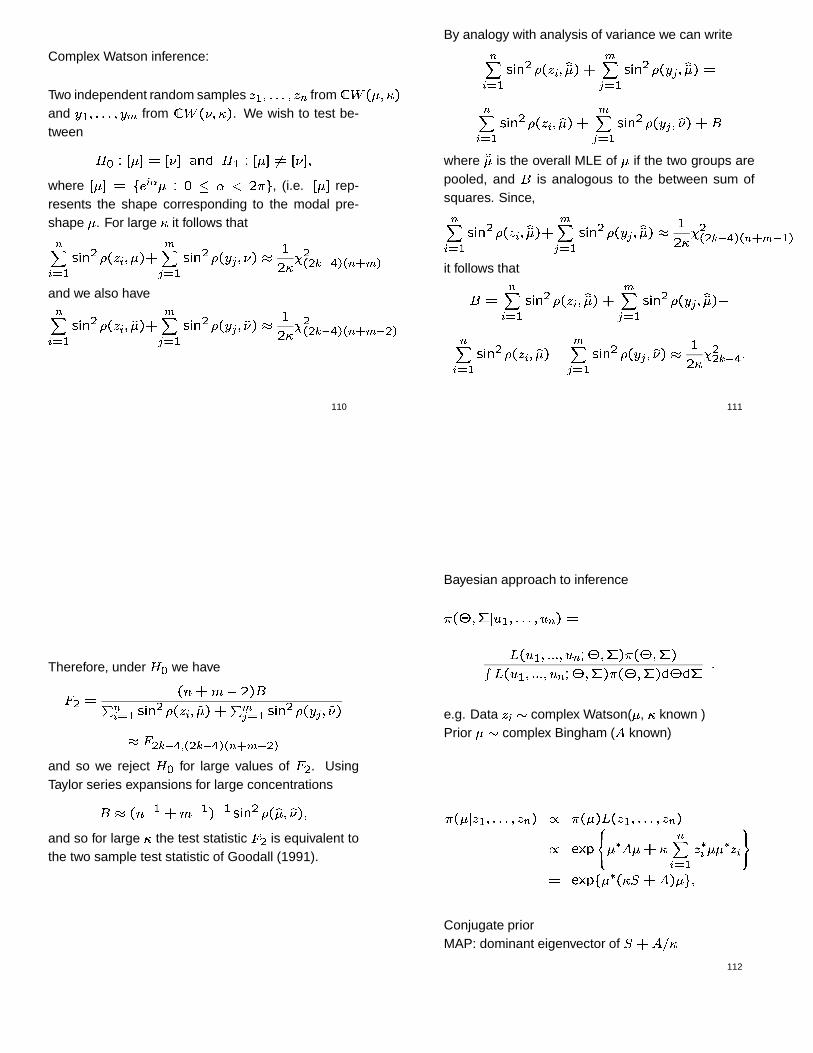
Complex Watson inference:
Two independent random samples j % 3 1 1 1 3 j Õ from 5 � � Ø 3 �and u % 3 1 1 1 3 u � from 5 � � / 3 � . We wish to test be-tween l S � � Ø � � � / � / � � l % � � Ø � Ó� � / � 3where
� Ø � � � � # 0 Ø � > y 1 { t z � , (i.e.
� Ø �rep-
resents the shape corresponding to the modal pre-shape
Ø. For large
it follows thatÕ"# $ % � � � ) ¹ � j # 3 Ø � o �"& $ % � � � ) ¹ � u & 3 / � í ,t � ) F ) � ; v I F Õ � � I
and we also haveÕ"# $ % � � � ) ¹ � j # 3 ÃØ � o �"& $ % � � � ) ¹ � u & 3 Ã/ � í ,t � ) F ) � ; v I F Õ � � ; ) I110
By analogy with analysis of variance we can writeÕ"# $ % � � � ) ¹ � j # 3 à ÃØ � o �"& $ % � � � ) ¹ � u & 3 à ÃØ � �Õ"# $ % � � � ) ¹ � j # 3 ÃØ � o �"& $ % � � � ) ¹ � u & 3 Ã/ � o æwhere à ÃØ
is the overall MLE ofØ
if the two groups arepooled, and æ is analogous to the between sum ofsquares. Since,Õ"# $ % � � � ) ¹ � j # 3 Ã ÃØ � o �"& $ % � � � ) ¹ � u & 3 Ã ÃØ � í ,t � ) F ) � ; v I F Õ � � ; % Iit follows thatæ � Õ"# $ % � � � ) ¹ � j # 3 Ã ÃØ � o �"& $ % � � � ) ¹ � u & 3 Ã ÃØ � 'Õ"# $ % � � � ) ¹ � j # 3 ÃØ � ' �"& $ % � � � ) ¹ � u & 3 Ã/ � í ,t � )) � ; v 1
111
Therefore, under l S we have ) � � Ô o � ' t � æ* Õ# $ % � � � ) ¹ � j # 3 ÃØ � o * �& $ % � � � ) ¹ � u & 3 Ã/ �í ) � ; v N F ) � ; v I F Õ � � ; ) Iand so we reject l S for large values of
) . UsingTaylor series expansions for large concentrationsæ í � Ô ; % o � ; % � ; % � � � ) ¹ � ÃØ 3 Ã/ � 3and so for large
the test statistic
) is equivalent tothe two sample test statistic of Goodall (1991).
Bayesian approach to inferencez � 2 3 � º 7 % 3 1 1 1 3 7 Õ � �3 � 7 % 3 1 1 1 3 7 Õ � 2 3 � � z � 2 3 � �4 3 � 7 % 3 1 1 1 3 7 Õ � 2 3 � � z � 2 3 � � � 2 � � 1e.g. Data j # � complex Watson(
Ø,
known )
PriorØ � complex Bingham ( � known)
z � Ø º j % 3 1 1 1 3 j Õ � ( z � Ø � 3 � j % 3 1 1 1 3 j Õ �( � � Û 56 7 Ø ½ � Ø o Õ"# $ % j ½# Ø Ø ½ j # 8 9:� � � Û � Ø ½ � � o � � Ø � 3Conjugate priorMAP: dominant eigenvector of
� o � r 112

The smoothed Procrustes mean of the T2 Small data:(Top left)
³ � > , (top right)³ � > 1 , , (bottom left)³ � , 1 > , (bottom right)
³ � , > > .
113
EDMA (Euclidean distance matrix analysis) [Lele, 91+,Stoyan, 91] � � � : form distance matrix (
� � �matrix of pairs of
inter-landmark distances (ILDs))
Estimate � Ø � : population form distance matrix� 2 & 3 u & � � � � � Ø & 3 / & � 3 � ) + ) � 3 @ � , 3 1 1 1 3 �
. Then� 2 ; ' 2 < � ) o � u ; ' u < � ) � 0 ); < � � ) � )) � = ); < r � ) � 3 (4)= ); < � � Ø ; ' Ø < � ) o � / ; ' / < � ) .
Moment estimator
= v; < � � � 0 ); < � � ) ' > / . � 0 ); < � 1Removes bias.
Estimate of mean reflection size-and-shape� � 0 � ) � ? � � 3 � ? � ; < � Ã= ; < 3114
EDMA-I test (Lele and Richtsmeier, 1991)
Form ratio distance matrix0 # & � � 3 * � � # & � � � r # & � * � 1 (5)
Test statistic:� � @ / �# N & 0 # & � ÃØ 3 Ã/ � r @ � �# N & 0 # & � ÃØ 3 Ã/ � 3 (6)
Use bootstrap procedures.
115
EDMA-II (Lele and Cole, 1995)
à ٠and à Aestimates of average form distance matrix
for each group
Scale by group size measure� = Largest entry in arithmetic difference of scaledmatrices
More powerful than EDMA-I
116
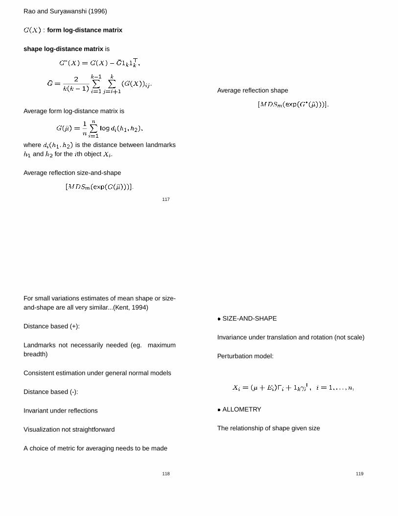
Rao and Suryawanshi (1996)B � � � : form log-distance matrix
shape log-distance matrix isB ½ � � � � B � � � ' (B , � , ¼ � 3(B � t� � � ' , � � ; %"# $ % �"& $ # � % � B � � � � # & 1Average form log-distance matrix isB � ÃØ � � ,Ô Õ"# $ % C � Å Æ # � � % 3 � ) � 3where
Æ # � � % 3 � ) � is the distance between landmarks� % and� ) for the p th object
� # .Average reflection size-and-shape� � 0 � � � � � Û � B � ÃØ � � � � 1
117
Average reflection shape� � 0 � � � � � Û � B ½ � ÃØ � � � � 1
For small variations estimates of mean shape or size-and-shape are all very similar...(Kent, 1994)
Distance based (+):
Landmarks not necessarily needed (eg. maximumbreadth)
Consistent estimation under general normal models
Distance based (-):
Invariant under reflections
Visualization not straightforward
A choice of metric for averaging needs to be made
118
� SIZE-AND-SHAPE
Invariance under translation and rotation (not scale)
Perturbation model:
� # � � Ø o # � � # o , � Ö ¼# 3 p � , 3 1 1 1 3 Ô 3� ALLOMETRY
The relationship of shape given size
119

Bookstein’s (1996) Microfossils
•
•
•
•
•
•
•
••
•
•
•
•
•
•••
•
•
•
•
U
V
V0.2 0.3 0.4 0.5 0.6
0.4
0.5
0.6
0.7
0.8
60
65
64
65
67
71
72
7174
75
76
84
84
84
878888
88
92
100
100
i � i 8 versush � h 8 o , r t
120
Microfossils:
slog
0.32 0.36 0.40 0.44
•
• •••
• ••• ••
•• •••••
•
• •
8.2
8.4
8.6
8.8
9.0X 9.
2
•
• • ••
•• •• ••
•• ••• •
•
• •
0.32
0.36
0.40
0.44
•
•
•
•
• •
•
•
•••
••• •
•
•
••
•
•
U
•
•
•
•
• •
•
•
•••
••
• ••
•
••
•
•
8.2 8.4 8.6 8.8 9.0 9.2D•
•
•
•
•
••
• •
••
•
•
••••
••
•
•
•
•
•
•
••
••
••
•
•
••••
•
••
•
0.45 0.55 0.65 0.75
0.45
0.55Y 0.
650.
75
V
Regression:h � 1 % o ¿ % C � Å � 3 i � 1 ) o ¿ ) C � Å �Tthe fitted values (with standard errors) areÃ1 % � > 1 Ò Ò � > 1 t > � , ÿ % � ' > 1 > � � > 1 > t � ,Ã1 ) � ' , 1 � Ò � > 1 A t � and ÿ ) � > 1 t � � > 1 > � �Significant linear relationship between C � Å �
and i .
121
T2 Small mouse vertebrae data
s
-0.10 -0.05 0.0 0.05
•
•
••
•
•
••
•
••
•
•
•
•
••
•
•
•
•
•
••
•
••
•
•
••
•
••
•
•
•
•
••
•
•
•
•
•
•
-0.02 0.0 0.02
165
170
175
180
185
•
•
••
•
•
••
•
••
•
•
•
•
••
•
•
•
•
•
•
-0.1
0-0
.05
0.0
0.05
•
•
•
•
•
•
•
•
•
•
•
•
•
•
•
•
•
•
•
•
•
•
•
PC1•
•
•
•
•
•
•
•
•
•
•
•
•
•
•
•
•
•
•
•
•
•
•
•
•
•
•
•
•
•
•
•
•
•
•
•
•
•
•
•
•
•
•
•
•
•
•
•
••
•
•
••
•
•
•
• •
•
•
•
•
•
••
•
••
•
•
••
•
•
••
•
•
•
• •
•
•
•
•
•
••
•
••
PC2
-0.0
4-0
.02
0.0
0.02
•
•
••
•
•
••
•
•
•
••
•
•
•
•
•
••
•
• •
165 170 175 180 185
-0.0
20.
00.
02
•
•
•
•
•
• •
•
••
••
•
•
•
•
•
•
•
•
•
•
•
•
•
•
•
•
• •
•
••
••
•
•
•
•
•
•
•
•
•
•
•
-0.04 -0.02 0.0 0.02
•
•
•
•
•
••
•
••
••
•
•
•
•
•
•
•
•
•
•
• PC3
NB: Approx. linear relationship between PC 1 andcentroid size.
122
Shapes package in R:
http://www.cran-r-project.org
Library of shape analysis routines.
Also see:
http://www.maths.nott.ac.uk/ � ild/shapes
123

Session III:� Deformations� Shape in images� Temporal shape� Shape Regression� Discussion
124
DEFORMATIONS AND THIN-PLATE SPLINES
The thin-plate spline is the most natural interpolant intwo dimensions because it minimizes the amount ofbending in transforming between two configurations,which can also be considered a roughness penalty.The theory of which was developed by Duchon (1976)and Meinguet (1979). Consider the
� t � , � landmarks� & 3 @ � , 3 1 1 1 3 �, on the first figure mapped exactly
into u # 3 p � , 3 1 1 1 3 �, on the second figure, i.e. there
aret �
interpolation constraints,� u & � ; � E ; � � & � 3 s � , 3 t 3 @ � , 3 1 1 1 3 � 3 (7)
and we write E � � & � � � E % � � & � 3 E ) � � & � � ¼ 3 @ � , 3 1 1 1 3 � 3for the two dimensional deformation. Let� � � � % � ) 1 1 1 � � � ¼ 3 * � � u % u ) 1 1 1 u � � ¼so that � and
*are both
� � � t � matrices.
A pair of thin-plate splines (PTPS) is given by thebivariate functionE � � � � � E % � � � 3 E ) � � � � ¼� ô o � � o � ¼ ò � � � 3 (8)
125
where�
is� t � , � 3 ò � � � � � � � � ' � % � 3 1 1 1 3 � � � ' � � � � ¼ 3 � � �, � and � � � � � Í � � � ) C � Å � � � � � 3 � � � � > 3> 3 � � � � > 1 (9)
Thet � o "
parameters of the mapping are ô � t �, � 3 � � t � t � and
� � � � t � . There aret �
interpola-tion constraints in Equation (7), and we introduce sixmore constraints in order for the bending energy inEquation (14) below to be defined:, ¼ � � � > 3 � ¼ � � > 1 (10)
The pair of thin-plate splines which satisfy the con-straints of Equation (10) are called natural thin-platesplines. Equations (7) and (10) can be re-written inmatrix formFGH � , � �, ¼ � > >� ¼ > > I JK FGH
�ô ¼� ¼ I JK � FGH * >> I JK 3 (11)
where� � � # & � � � � # ' � & � and , � is the
�-vector of
ones. The matrix� � FGH � , � �, ¼ � > >� ¼ > > I JKis symmetric positive definite and so the inverse ex-ists, provided the inverse of
�exists. Hence,FGH
�ô ¼� ¼ I JK � FGH � , � �, ¼ � > >� ¼ > > I JK ; % FGH * >> I JK � � ; % FGH * >> I JK 3
say. Writing the partition of � ; %as� ; % � L � % % � % )� ) % � ) ) M 3
where � % %is
� � �, it follows that
� � � % % *L ô ¼� ¼ M � � ÿ % 3 ÿ ) � � � ) % * 3 (12)
giving the parameter values for the mapping. If� ; %

exists, then we have� % % � � ; % ' � ; % N � N ¼ � ; % N � ; % N ¼ � ; % 3� ) % � � N ¼ � ; % N � ; % N ¼ � ; % � � � % ) � ¼ 3 (13)� ) ) � ' � N ¼ � ; % N � ; % 3where
N � � , � 3 � �, using for example Rao (1973,p39).
Using Equations (12) and (13) we see that ÿ % and ÿ )are generalized least squares estimators, and� � > � � ÿ % 3 ÿ ) � ¼ � � ' � ) ) 1Mardia et al. (1991) gave the expressions for the casewhen
�is singular.
The� � �
matrix æ O is called the bending energymatrix where æ O � � % % 1 (14)
There are three constraints on the bending energymatrix , ¼ � æ O � > 3 � ¼ æ O � >
and so the rank of the bending energy matrix is� ' A .
It can be proved that the transformation of Equation(8) minimizes the total bending energy of all possibleinterpolating functions mapping from � to
*, where
the total bending energy is given byP � E � �)"& $ % Q Q R S = � T ) E &T 2 ) � ) o t � T ) E &
T 2 T u � ) o � T ) E &T u ) � ) � 2 � u 1
(15)A simple proof is given by Kent and Mardia (1994a).The minimized total bending energy is given by,P � E � � � . / � � � � ¼ � � � � � . / � � � * ¼ � % % * � 1
(16)
In calculating a deformation grid we do not want tosee any more bending locally than is necessary andalso do not want to see bending where there are nodata.
Early transformation grids of human profiles
126
Early transformation grids modelling six stages throughlife (from Medawar, 1944).
127

TRANSFORMATION GRIDS
Following from the original ideas of D’Arcy Thompson(1917) we can produce similar transformation grids,using a pair of thin-plate splines for the deformationfrom configuration matrices � to
*.
(a) (b)
128
A regular square grid is drawn over the first figure andat each point where two lines on the grid meet
� # thecorresponding position in the second figure is calcu-lated using a pair of thin-plate splines transformationu # � E � � # � 3 p � , 3 1 1 1 3 Ô U , where Ô U is the numberof junctions or crossing points on the grid. The junc-tion points are joined with lines in the same order asin the first figure, to give a deformed grid over the sec-ond figure. The pair of thin-plate splines can be usedto produce a transformation grid, say from a regularsquare grid on the first figure to a deformed grid onthe second figure. The resulting interpolant producestransformation grids that ‘bend’ as little as possible.We can think of each square in the deformation as be-ing deformed into a quadrilateral (with four shape pa-rameters). The PTPS minimizes the local variation ofthese small quadrilaterals with respect to their neigh-bours.
Considerdescribingthesquaretokite transformationwhich
wasconsideredbyBookstein(1989)andMardiaandGoodall
(1993).Given� � �
pointsin � � tdimensionsthema-
trices � and*
aregivenby
� � FGGGH > ,' , >> ' ,, >I JJJK 3 * � FGGGH > > 1 Ò ?' , > 1 t ?> ' , 1 t ?, > 1 t ?
I JJJK 1Wehavehere � �
FGGGGH > � ¾ �� > � ¾¾ � > �� ¾ � >I JJJJK 3
where� � � � ! t � � > 1 " ! A , and ¾ � � � t � �t 1 Ò Ò t ". In thiscase,thebendingenergy matrix is
æ O � � % % � > 1 , Ñ > A FGGGH , ' , , ' ,' , , ' , ,, ' , , ' ,' , , ' , ,I JJJK 1
129
It is foundthat� ¼ � L > > > >' > 1 , Ñ > A > 1 , Ñ > A ' > 1 , Ñ > A > 1 , Ñ > A M 3(17)ô � > 3 � � + )andso the pair of thin-platesplinesis given by E � � � �� E % � � � 3 E ) � � � � ¼ , whereE % � � � � � � , � 3 (18)E ) � � � � � � t � o > 1 , Ñ > A v"& $ % � ' , � & � � � � ' � & � � 1NotethatEquation(18) is asexpected,becausethereis no
changein the� � , �
direction. The affine part of the defor-
mationis theidentity transformation.

-2 -1 0 1 2
-2-1
01
2
••
••
-2 -1 0 1 2
-2-1
01
2
••
•
•
-2 -1 0 1 2
-2-1
01
2
••
• •
-2 -1 0 1 2
-2-1
01
2
••
• •
Transformationgrids for the square(left column) to kite
(right column)(afterBookstein,1989). In thesecondrow
thesamefiguresasin thefirst row havebeenrotatedby� ? m
andthedeformedgrid doeslook different,eventhoughthe
transformationis thesame.
WeconsiderThompson-likegridsfor thisexample(above).
A regular squaregrid is placedon the first figure andde-
formedinto thecurvedgrid on thekite figure. We seethat
thetopandbottommostpointsaremoveddownwardswith
respectto theothertwo points.If theregulargrid is drawn
on the first figure at a different orientation,then the de-
formedgrid doesappearto be different,even thoughthe
transformationis thesame.Thiseffect is seenin theFigure
wherebothfigureshave beenrotatedclockwiseby� ? m in
thesecondrow.
-0.6 -0.4 -0.2 0.0
(a)
0.2 0.4 0.6
-0.6
-0.4
-0.2
0.0
0.2
0.4
0.6
••
•
•
••••
••••
•
-0.6 -0.4 -0.2 0.0
(b)
0.2 0.4 0.6
-0.6
-0.4
-0.2
0.0
0.2
0.4
0.6
••
•
•
••••
••••
•
A thin-plate spline transformation grid between the con-trol mean shape estimate and the schizophrenia meanshape estimate.
(left) We see a square grid drawn on the estimate ofmean shape for the Control group in the schizophreniastudy. Here there are Ô U � A > � t ! � Ñ Ò > junctionsand there are
� � , A landmarks. (right) we see theschizophrenia mean shape estimate and the grid ofnew points obtained from the PTPS transformation.It is quite clear that there is a shape change in thecentre of the brain, around landmarks 1, 9 and 13.
130
6000 7000 8000 9000 10000 11000 12000
8000
9000
1000
011
000
1200
013
000
•••• •
•••••••
6000 7000 8000 9000 10000 11000 12000
8000
9000
1000
011
000
1200
013
000
••••
••
••••••
6000 7000 8000 9000 10000 11000 12000
8000
9000
1000
011
000
1200
013
000
•••• •
•••••••
6000 7000 8000 9000 10000 11000 12000
8000
9000
1000
011
000
1200
013
000
•••• •
•••••••
6000 7000 8000 9000 10000 11000 12000
8000
9000
1000
011
000
1200
013
000
•••• •
•••••••
A series of grids showing the shape changes in theskull of some sooty mangabey monkeys
131

PRINCIPAL AND PARTIAL WARPS
Bookstein (1989, 1991)’s principal and partial warpsare useful for decomposing the thin-plate spline trans-formations into a series of large scale and small scalecomponents.
Consider the pair of thin-plate splines transformationfrom
� 4 ) to u 4 ) , which interpolates the�
points � to*
(� � t
) matrices. An eigen-decompositionof the
� � �bending energy matrix æ O of Equation (14)
has non-zero eigenvalues³ % y ³ ) y 1 1 1 y ³ � ; P
with corresponding eigenvectors Ö % 3 Ö ) 3 1 1 1 3 Ö � ; P . Theeigenvectors Ö % 3 Ö ) 3 1 1 1 3 Ö � ; P are called the princi-pal warp eigenvectors and the eigenvalues are calledthe bending energies. The functions,� & � � � � Ö ¼& ò � � � 3 @ � , 3 1 1 1 3 � ' A 3are the principal warps, where ò � � � � � � � � ' � % � 3 1 1 1 3 � � � '� � � � ¼ .
132
Here we have labelled the eigenvalues and eigenvec-tors in this order (with
³ % as the smallest eigenvaluecorresponding to the first principal warp) to follow Book-stein’s (1996b) labelling of the order of the warps. Theprincipal warps do not depend on the second figure
*.
The principal warps will be used to construct an or-thogonal basis for re-expressing the thin-plate splinetransformations. The principal warp deformations areunivariate functions of two dimensional
�, and so could
be displayed as surfaces above the plane or as con-tour maps. Alternatively one could plot the transfor-mation grids from
�to u � � o � ô % � & � � � 3 ô ) � & � � � � ¼
for each@, for particular values of ô % and ô ) . Note that
the principal warps are orthonormal.
The partial warps are defined as the set of� ' A
bivariate functions é & � � � 3 @ � , 3 1 1 1 3 � ' A , whereé & � � � � * ¼ ³ & Ö & � & � � � � * ¼ ³ & Ö & Ö ¼& ò � � � 1The
@th partial warp scores for
*(from � ) are de-
fined as� ó & % 3 ó & ) � ¼ � * ¼ Ö & 3 @ � , 3 1 1 1 3 � ' A 3
and so there are two scores for each partial warp.
Since � ¼ ò � � � � � ; P"& $ % é & � � � 3we see that the non-affine part of the pair of thin-platesplines transformation can be decomposed into thesum of the partial warps. The
@th partial warp cor-
responds largely to the movement of the landmarkswhich are the most highly weighted in the
@th prin-
cipal warp. The@th partial warp scores indicate the
contribution of the@th principal warp to the deforma-
tion from the source � to the target*
, in each of theCartesian axes.
-0.6 -0.4 -0.2 0.0 0.2 0.4 0.6
-0.6
-0.4
-0.2
0.0
0.2
0.4
0.6
• •••••
• •
-0.6 -0.4 -0.2 0.0 0.2 0.4 0.6
-0.6
-0.4
-0.2
0.0
0.2
0.4
0.6
• ••••
•• •
-0.6 -0.4 -0.2 0.0 0.2V
0.4 0.6
-0.6
-0.4
-0.2
0.0
0.2
0.4
0.6
• ••••
•• •
-0.6 -0.4 -0.2 0.0 0.2 0.4 0.6
-0.6
-0.4
-0.2
0.0
0.2
0.4
0.6
••
••••
• •
-0.6 -0.4 -0.2 0.0 0.2 0.4 0.6
-0.6
-0.4
-0.2
0.0
0.2
0.4
0.6
• ••••
•• •
The five principal warps for the the pooled mean shapeof the gorillas
133

-0.6 -0.4 -0.2 0.0
(a)
0.2 0.4 0.6
-0.6
-0.4
-0.2
0.0
0.2
0.4
0.6
• ••••
•• •
-0.6 -0.4 -0.2 0.0
(b)
0.2 0.4 0.6-0
.6-0
.4-0
.20.
00.
20.
40.
6
• ••••
•• •
A thin-plate spline transformation grid between a fe-male and a male gorilla skull midline.
134
-0.6 -0.4 -0.2 0.0 0.2 0.4 0.6
-0.6
-0.4
-0.2
0.0
0.2
0.4� 0.
6
• •••••
• •
-0.6 -0.4 -0.2 0.0 0.2ö
0.4 0.6
-0.6
-0.4
-0.2
0.0
0.2
0.4� 0.
6
• ••••
•• •
-0.6 -0.4 -0.2 0.0 0.2 0.4 0.6
-0.6
-0.4
-0.2
0.0
0.2
0.4� 0.
6
• ••••
•• •
-0.6 -0.4 -0.2 0.0 0.2 0.4 0.6
-0.6
-0.4
-0.2
0.0
0.2
0.4
0.6
• •••••
• •
-0.6 -0.4 -0.2 0.0 0.2ö
0.4 0.6
-0.6
-0.4
-0.2
0.0
0.2
0.4
0.6
• •••••
• •
-0.6 -0.4 -0.2 0.0 0.2 0.4 0.6
-0.6
-0.4
-0.2
0.0
0.2
0.4
0.6
• •••••
• •
Affine and partial warps for Gorilla (Female to malemean shapes)
135
f
f
f
f
ff
f
ff
f
f f
f
f
f
fff
ff
ff
f
f
f
f
f
f
f f
-0.06 -0.04 -0.02 0.0 0.02 0.04 0.06
-0.0
6-0
.04
-0.0
20.
00.
020.
040.
06
m
mm
mmm
m
mm
mmm
mm
mm
mm
m
m
m
m
m
m
m
m m
m
m
f
ff
f
f f
f
ff
f
ff
ff
f
f
f
f
f
f
f
f
f
f
f
ff
f
f
f
-0.06 -0.04 -0.02 0.0 0.02 0.04 0.06
-0.0
6-0
.04
-0.0
20.
00.
020.
040.
06
mm
mm
m
m
mm mm
mm
m
m
m
m
m
mm
m
m
m
mm
m
m
m
m
m
f
f
f
f
fff
f f
f
ff
f
f
f
f
ff
f
ff
f
f
f ff f
f ff
-0.06 -0.04 -0.02 0.0 0.02 0.04 0.06
-0.0
6-0
.04
-0.0
20.
00.
020.
040.
06
mm
mm
m
m
m
m
m
m
m
m
m
m
m m
m
m
mm m
mm
m
mmm
m
m
f
ff
f
f
f
f
f
ff
ff
f
fff
f
ff
f
f
f
ff
ff
f
f
ff
-0.06 -0.04 -0.02 0.0 0.02 0.04 0.06
-0.0
6-0
.04
-0.0
20.
00.
020.
040.
06
m
m
m
mm
m
m
m
m
m
m
mmm
mm
m
m
mmmm
m mmm m
mm f
f
fff
f
fff
ff
f
f
ff
ff
f
f
f
ff
f
fff
ff
ff
-0.06 -0.04 -0.02 0.0 0.02 0.04 0.06
-0.0
6-0
.04
-0.0
20.
00.
020.
040.
06
mm m
m
mm
mm
m
mmm
mm
mm
mm
m
m
m
mm
m
mmm
m
m
f
f
f
ff
f f
ff
fff
fff
fff f
fff
f f
ffff
f
f
-0.06 -0.04 -0.02 0.0 0.02 0.04 0.06
-0.0
6-0
.04
-0.0
20.
00.
020.
040.
06
mmm
m
mm m
m
mm
m
mmm
mm
mm mmmm
mmmm
m
m
m
Affine scores and the partial warp scores for female(f) and male (m) gorilla skulls.
136
RELATIVE WARPS
Principal component analysis with non-Euclidean met-rics
Define the pseudo-metric space� è 3 Æ ð � as the realó -vectors with pseudo-metric given byÆ ð � 2 % 3 2 ) � � W � 2 % ' 2 ) � ¼ � ; � 2 % ' 2 ) � 3
where 2 % and 2 ) are ó -vectors, and � ; is a gener-alized inverse (or inverse if it exists) of the positivesemi-definite matrix � .
The Moore–Penrose inverse is a suitable choice ofgeneralized inverse. If � is the population covariancematrix of 2 % and 2 ) , then
Æ ð � 2 % 3 2 ) � is the Maha-lanobis distance. The norm of a vector 2 in the metricspace is � 2 � ð � Æ ð � 2 3 > � � � 2 ¼ � ; 2 � % L ) 1We could carry out statistical inference in the metricspace rather than in the usual Euclidean
� � � + �137
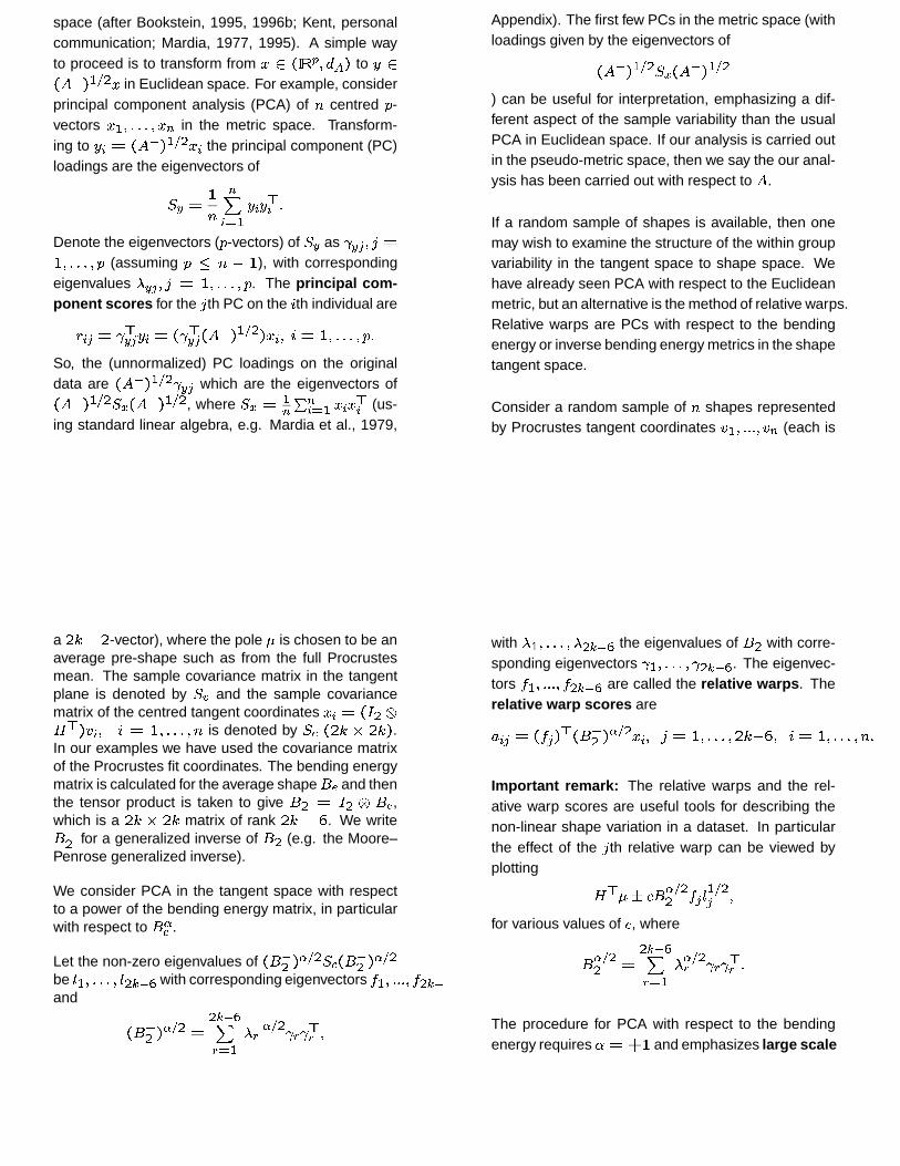
space (after Bookstein, 1995, 1996b; Kent, personalcommunication; Mardia, 1977, 1995). A simple wayto proceed is to transform from 2 4 � è 3 Æ ð � to u 4� � ; � % L ) 2 in Euclidean space. For example, considerprincipal component analysis (PCA) of Ô centred ó -vectors 2 % 3 1 1 1 3 2 Õ in the metric space. Transform-ing to u # � � � ; � % L ) 2 # the principal component (PC)loadings are the eigenvectors of� J � ,Ô Õ"# $ % u # u ¼# 1Denote the eigenvectors (ó -vectors) of
� J as Ö J & 3 @ �, 3 1 1 1 3 ó (assuming ó y Ô ' , ), with correspondingeigenvalues
³ J & 3 @ � , 3 1 1 1 3 ó . The principal com-ponent scores for the
@th PC on the p th individual ares # & � Ö ¼J & u # � � Ö ¼J & � � ; � % L ) � 2 # 3 p � , 3 1 1 1 3 ó 1
So, the (unnormalized) PC loadings on the originaldata are
� � ; � % L ) Ö J & which are the eigenvectors of� � ; � % L ) � 9 � � ; � % L ) , where� 9 � %Õ * Õ# $ % 2 # 2 ¼# (us-
ing standard linear algebra, e.g. Mardia et al., 1979,
Appendix). The first few PCs in the metric space (withloadings given by the eigenvectors of� � ; � % L ) � 9 � � ; � % L )) can be useful for interpretation, emphasizing a dif-ferent aspect of the sample variability than the usualPCA in Euclidean space. If our analysis is carried outin the pseudo-metric space, then we say the our anal-ysis has been carried out with respect to � .
If a random sample of shapes is available, then onemay wish to examine the structure of the within groupvariability in the tangent space to shape space. Wehave already seen PCA with respect to the Euclideanmetric, but an alternative is the method of relative warps.Relative warps are PCs with respect to the bendingenergy or inverse bending energy metrics in the shapetangent space.
Consider a random sample of Ô shapes representedby Procrustes tangent coordinates q % 3 1 1 1 3 q Õ (each is
at � ' t
-vector), where the poleØ
is chosen to be anaverage pre-shape such as from the full Procrustesmean. The sample covariance matrix in the tangentplane is denoted by
� O and the sample covariancematrix of the centred tangent coordinates 2 # � � + ) Xl ¼ � q # 3 p � , 3 1 1 1 3 Ô is denoted by
� ¸ � t � � t � � .In our examples we have used the covariance matrixof the Procrustes fit coordinates. The bending energymatrix is calculated for the average shape æ O and thenthe tensor product is taken to give æ ) � + ) X æ O ,which is a
t � � t �matrix of rank
t � ' ". We writeæ ;) for a generalized inverse of æ ) (e.g. the Moore–
Penrose generalized inverse).
We consider PCA in the tangent space with respectto a power of the bending energy matrix, in particularwith respect to æ 0O .
Let the non-zero eigenvalues of� æ ;) � 0 L ) � ¸ � æ ;) � 0 L )
be Y % 3 1 1 1 3 Y ) � ; # with corresponding eigenvectors ç % 3 1 1 1 3 ç ) � ;and � æ ;) � 0 L ) � ) � ; #"; $ % ³ ; 0 L ); Ö ; Ö ¼; 3
with³ % 3 1 1 1 3 ³ ) � ; # the eigenvalues of æ ) with corre-
sponding eigenvectors Ö % 3 1 1 1 3 Ö ) � ; # . The eigenvec-tors ç % 3 1 1 1 3 ç ) � ; # are called the relative warps. Therelative warp scores are� # & � � ç & � ¼ � æ ;) � 0 L ) 2 # 3 @ � , 3 1 1 1 3 t � ' " 3 p � , 3 1 1 1 3 Ô 1Important remark: The relative warps and the rel-ative warp scores are useful tools for describing thenon-linear shape variation in a dataset. In particularthe effect of the
@th relative warp can be viewed by
plotting l ¼ Ø Z ô æ 0 L )) ç & Y % L )& 3for various values of ô , whereæ 0 L )) � ) � ; #"; $ % ³ 0 L ); Ö ; Ö ¼; 1The procedure for PCA with respect to the bendingenergy requires 1 � o , and emphasizes large scale

variability. PCA with respect to the inverse bend-ing energy requires 1 � ' , and emphasizes smallscale variability. If 1 � > , then we take æ S) � + ) �as the
t � � t �identity matrix and the procedure is
exactly the same as PCA of the Procrustes tangentcoordinates. Bookstein (1996b) has called the 1 � >case PCA with respect to the Procrustes metric.
fff
f
fff
f
f
ff
f
f
f
f
fff
f ff
f
ff
fff
f f f
-0.06 -0.02 0.0 0.020.040.06-0
.06
-0.0
20.
00.
020.
040.
06
mm
m
mm mmm
mmmm
mmmmm
m
mmm
m mm
mmm
mm
-0.6 -0.4 -0.2 0.0
(a)
0.2 0.4 0.6
-0.6
-0.4
-0.2
0.0
0.2
0.4
0.6
• •••••
• •
-0.6 -0.4 -0.2 0.0
(b)
0.2 0.4 0.6
-0.6
-0.4
-0.2
0.0
0.2
0.4
0.6
• ••••
•
• •
Relative warps: 1 � ,
-0.6 -0.4 -0.2 0.0
(a)
0.2 0.4 0.6
-0.6
-0.4
-0.2
0.0
0.2
0.4
0.6
++
++++
+ +
-0.6 -0.4 -0.2 0.0
(b)
0.2 0.4 0.6
-0.6
-0.4
-0.2
0.0
0.2
0.4
0.6
++
++++
+ +
Deformation grids for the two uniform/affine vectorsfor the gorilla data.
138
f
ff
f
f
fff
ff
ff f
fff
fff
f
fff ff
f fff
f
-0.15 -0.050.0 0.050.100.15
-0.1
5-0
.05
0.0
0.05
0.10
0.15
m
m
m
mm
m
m
mmm
mm
mm
m
m
m
m
m
mmm
m
mm
m
m
m
m
-0.6 -0.4 -0.2 0.0
(a)
0.2 0.4 0.6
-0.6
-0.4
-0.2
0.0
0.2
0.4
0.6
• ••
•••• •
-0.6 -0.4 -0.2 0.0
(b)
0.2 0.4 0.6
-0.6
-0.4
-0.2
0.0
0.2
0.4
0.6
••
••••
• •
Relative warps: 1 � ' ,139
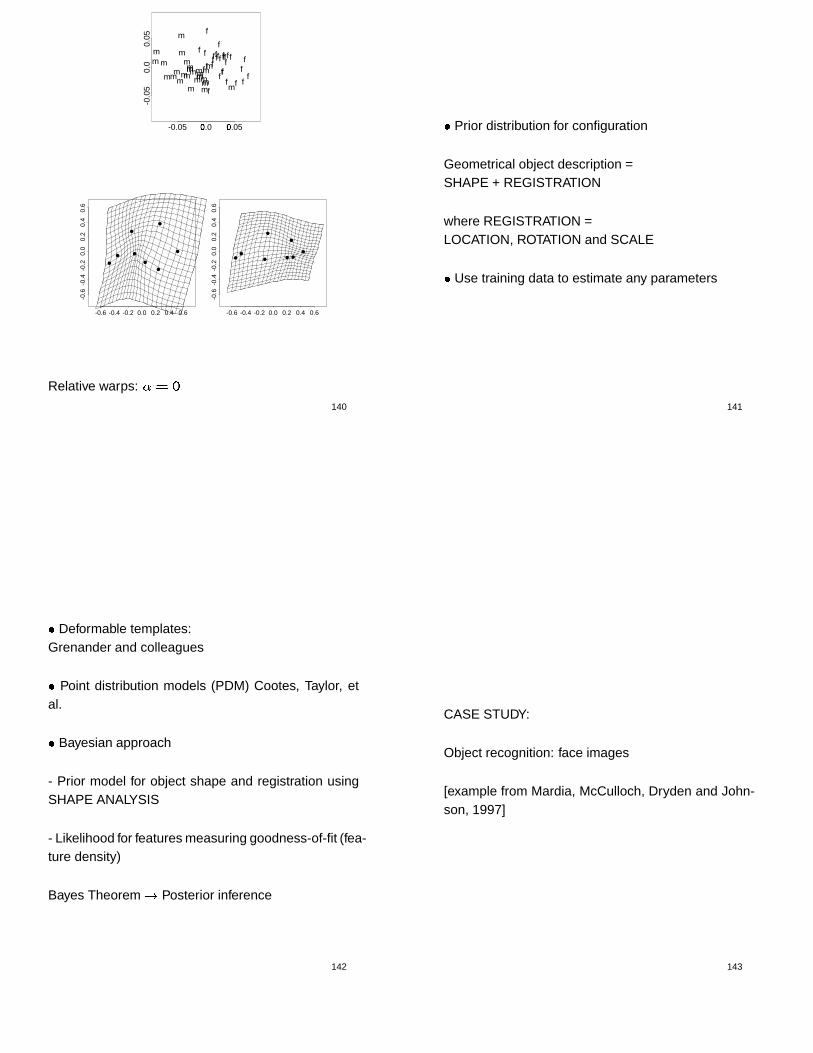
f
f f
f
f f ff
f
ff f
f
f
f
ff
ff
f
f
f
f
ff
fff f
f
-0.05 0.0
[0.05
[-0.0
50.
00.
05
m m
mmm mm m
mm m
mmmm
m
m
m
m
mmm mm
mm
m
m
m
-0.6 -0.4 -0.2 0.0 0.2 0.4 0.6
-0.6
-0.4
-0.2
0.0
0.2
0.4
0.6
••
••••
••
-0.6 -0.4 -0.2 0.0 0.2 0.4 0.6
-0.6
-0.4
-0.2
0.0
0.2
0.4
0.6
• •••••
• •
Relative warps: 1 � >140
� Prior distribution for configuration
Geometrical object description =SHAPE + REGISTRATION
where REGISTRATION =LOCATION, ROTATION and SCALE� Use training data to estimate any parameters
141
� Deformable templates:Grenander and colleagues� Point distribution models (PDM) Cootes, Taylor, etal.� Bayesian approach
- Prior model for object shape and registration usingSHAPE ANALYSIS
- Likelihood for features measuring goodness-of-fit (fea-ture density)
Bayes Theorem � Posterior inference
142
CASE STUDY:
Object recognition: face images
[example from Mardia, McCulloch, Dryden and John-son, 1997]
143

LANDMARKS or FEATURES� Grey level image + � 2 3 u �� Scale space features (e.g. Val Johnson, Duke; StephenPizer et al, UNC Chapel Hill, USA)
Convolution of image with isotropic bivariate Gaussiankernel at a succession of ‘scales’ ( � )
� � 2 3 u � � � �Q + � 2 ' � % 3 u ' � ) � ,t z � ) � ; <= \ = F ] = < � ] == I Æ � % Æ � )
Use 2D FFT� ‘Medialness’ : Laplacian of blurred scale space im-age
144
3 9 9 � � � o 3 J J � � � � T ) � � 2 3 u � � �T 2 ) o T ) � � 2 3 u � � �T u )
Pilot study - Face Identification: Choose� � !
land-marks on the medialness image at scales 8, 11, 13
145
� Feature density (likelihood)
3 � � @ / Å � º � � � ^ Å Ú . / � � � � � ( �_# $ % � <= ` × F ñ a × a × � ñ b × b × I� Johnson et al. (1997) motivate this as mimicking ahuman observer.� Features are treated as independent� High medialness at feature � high density� Treat non-feature grey levels as independent, uni-formly distributed (like a human observer ignoring thosepixels).� Parameters
# need to be specified
146

Registration parameters� LocationØ 9 � � � � 9 3 � )9 �Ø J � � � � J 3 � )J �� Rotationw � � � � c 3 � )c �� Isotropic scale¿ � � � � Ë 3 � )Ë �Hyperparameters � 9 3 � 9 3 � J 3 � J 3 � c 3 � c 3 � Ë 3 � Ë estimatedfrom training data (10 faces)
147
Original raw face data
• •
• •
•• •
••
x
yd0 50 100 150 200
050
100
150
200
1 2
3 4
56 7
81
x
yd0 50 100 150 200
050
100
150
200
1 2
3 4
5e
6 7
89f1 2
3 4g5
6 7
89
1 2
3 4
56 7
89
1 2
3h 4
g56 7
89
1 2
3 4
5
6 7
89
1 2
3 4
56 7
89
1 2
3 4
56 7
89
1 2
3 4
56 7
89
1 2
3 4
56 7
89
1 2
3h
4
56 7
89
148
Bookstein registered data
• •
• •
•
• •
••
u
vi-0.5 0.0 0.5
-1.5
-1.0
-0.5
0.0 • •
• •
•
• •
••
• •
• •
•
• •
••
• •
••
•
• •
••
• •
••
•
• •
••
• •
••
•
• •
••
• •
• •
•
• •
••
• •
• •
•• •
• •
• •
• •
•
• •
•
•
• •
• •
••
•
••
• •
• •
•
• •
••
149
� Least squares Procrustes approach
• •
• •
•
• •
••
-0.4 -0.2 0.0 0.2 0.4
-0.4
-0.2
0.0
0.2
0.4 • •
• •
•
• •
••
• •
• •
•
• •
••
• •
••
•
• •
••
• •
••
•
• •
••
••
• •
•
• •
••
• •
••
•
• •
••
• •
• •
•• •
• •
• •
••
•
• •
•
•
• •
• •
••
•
••
• •
••
•
• •
••
150
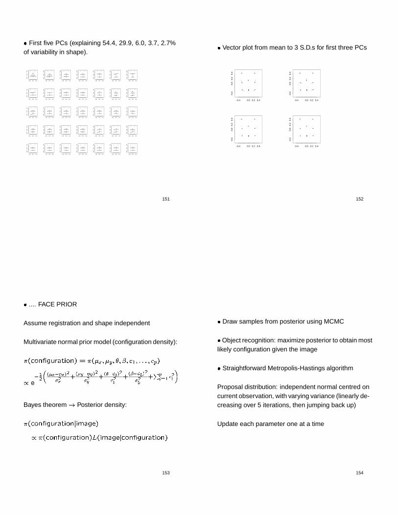
� First five PCs (explaining 54.4, 29.9, 6.0, 3.7, 2.7%of variability in shape).
• •
• •
•
• •••
-0.4 0.0 0.4
-0.4
0.0
0.4 • •
• •
•
• •
••
-0.4 0.0 0.4
-0.4
0.0
0.4 • •
• •
•• •
••
-0.4 0.0 0.4
-0.4
0.0
0.4 • •
• •
•• •
••
-0.4 0.0 0.4
-0.4
0.0
0.4 • •
• •
•• •
••
-0.4 0.0 0.4
-0.4
0.0
0.4 • •
• •
•• •
••
-0.4 0.0 0.4
-0.4
0.0
0.4 • •
• •
•• •
••
-0.4 0.0 0.4
-0.4
0.0
0.4
• •
• •
•• •
••
-0.4 0.0 0.4
-0.4
0.0
0.4
• •
• •
•• •
••
-0.4 0.0 0.4
-0.4
0.0
0.4 • •
• •
•• •
••
-0.4 0.0 0.4
-0.4
0.0
0.4 • •
• •
•• •
••
-0.4 0.0 0.4
-0.4
0.0
0.4 • •
• •
•• •
••
-0.4 0.0 0.4
-0.4
0.0
0.4 • •
• •
•• •
••
-0.4 0.0 0.4
-0.4
0.0
0.4 • •
• •
•
• •
••
-0.4 0.0 0.4
-0.4
0.0
0.4
• •
• •
•• •
••
-0.4 0.0 0.4
-0.4
0.0
0.4 • •
• •
•• •
••
-0.4 0.0 0.4
-0.4
0.0
0.4 • •
• •
•• •
••
-0.4 0.0 0.4
-0.4
0.0
0.4 • •
• •
•• •
••
-0.4 0.0 0.4
-0.4
0.0
0.4 • •
• •
•• •
•
-0.4 0.0 0.4
-0.4
0.0
0.4 • •
• •
•• •
••
-0.4 0.0 0.4
-0.4
0.0
0.4 • •
• •
•• •
••
-0.4 0.0 0.4
-0.4
0.0
0.4
• •
• •
•• •
••
-0.4 0.0 0.4
-0.4
0.0
0.4 • •
• •
•• •
••
-0.4 0.0 0.4
-0.4
0.0
0.4 • •
• •
•• •
••
-0.4 0.0 0.4
-0.4
0.0
0.4 • •
• •
•• •
••
-0.4 0.0 0.4
-0.4
0.0
0.4 • •
• •
•• •
••
-0.4 0.0 0.4
-0.4
0.0
0.4 • •
• •
•• •
••
-0.4 0.0 0.4
-0.4
0.0
0.4 • •
• •
•• •
••
-0.4 0.0 0.4
-0.4
0.0
0.4
• •
• •
•• •
••
-0.4 0.0 0.4
-0.4
0.0
0.4 • •
• •
•• •
••
-0.4 0.0 0.4
-0.4
0.0
0.4 • •
• •
•• •
••
-0.4 0.0 0.4
-0.4
0.0
0.4 • •
• •
•• •
••
-0.4 0.0 0.4
-0.4
0.0
0.4 • •
• •
•• •
••
-0.4 0.0 0.4
-0.4
0.0
0.4 • •
• •
•• •
••
-0.4 0.0 0.4
-0.4
0.0
0.4
• •
• •
•• •
••
-0.4 0.0 0.4
-0.4
0.0
0.4
151
� Vector plot from mean to 3 S.D.s for first three PCs
• •
• •
•• •
••
-0.4 0.0 0.2 0.4
-0.4
0.0
0.2
0.4 • •
• •
•• •
••
-0.4 0.0 0.2 0.4
-0.4
0.0
0.2
0.4
• •
• •
•• •
••
-0.4 0.0 0.2 0.4
-0.4
0.0
0.2
0.4 • •
• •
•• •
••
-0.4 0.0 0.2 0.4
-0.4
0.0
0.2
0.4
152
� .... FACE PRIOR
Assume registration and shape independent
Multivariate normal prior model (configuration density):z � � � � ^ Å Ú . / � � � � � � z � Ø 9 3 Ø J 3 w 3 ¿ 3 ô % 3 1 1 1 3 ô è �( � ; <= } j k a ) l a m =\ =a � j k b ) l b m =\ =b � j n ) l o m =\ =o � j p ) l q m =\ =q � * r × s < ¸ =× ~Bayes theorem � Posterior density:z � � � � ^ Å Ú . / � � � � º � @ / Å � �( z � � � � ^ Å Ú . / � � � � � 3 � � @ / Å � º � � � ^ Å Ú . / � � � � �
153
� Draw samples from posterior using MCMC� Object recognition: maximize posterior to obtain mostlikely configuration given the image� Straightforward Metropolis-Hastings algorithm
Proposal distribution: independent normal centred oncurrent observation, with varying variance (linearly de-creasing over 5 iterations, then jumping back up)
Update each parameter one at a time
154

Results: MCMC output for face 2 (in training set): Pos-terior, Prior, Likelihood
1:nsim
chai
nsp
0 500t
1000 1500 2000u
2500u90
0v 950
1000
1050
1100
1150
1:nsim
chai
nspr
0 500t
1000 1500 2000u
2500u-1
0-8
-6-4
-2
1:nsim
chai
nsli
0 500t
1000 1500 2000u
2500u90
095
010
0010
5011
0011
5012
00
155
Translations, scale, rotation, PC1, PC2
1:nsim
chai
nsx[
i, ]
0 500t
1000 1500 2000u
2500u12
813
213
6
1:nsim
chai
nsx[
i, ]
0 500t
1000 1500 2000u
2500u78w 80x 82x 84x
1:nsim
chai
nsx[
i, ]
0 500t
1000 1500 2000u
2500u90v 94
98
1:nsim
chai
nsx[
i, ]
0 500t
1000 1500 2000u
2500u-0
.04
0.0
0.04
1:nsim
chai
nsx[
i, ]
0 500t
1000 1500 2000u
2500u-0
.80.
0
1:nsim
chai
nsx[
i, ]
0 500t
1000 1500 2000u
2500u-1
.5-0
.5
156
PC3,...,PC8
1:nsim
chai
nsx[
i + 6
, ]
0 500t
1000 1500 2000u
2500u0.
01.
02.
0
1:nsim
chai
nsx[
i + 6
, ]
0 500t
1000 1500 2000u
2500u-2
.5-1
.0
1:nsim
chai
nsx[
i + 6
, ]
0 500t
1000 1500 2000u
2500u-1
.50.
01.
5
1:nsim
chai
nsx[
i + 6
, ]
0 500t
1000 1500 2000u
2500u-0
.51.
02.
0y1:nsim
chai
nsx[
i + 6
, ]
0 500t
1000 1500 2000u
2500u-1
01
2
1:nsim
chai
nsx[
i + 6
, ]
0 500t
1000 1500 2000u
2500u-1
01
2
157
MAP estimate overlaid on scale 8
0 50 100 150 200 250
050
100
150
200
250
S S
S S
SS S
SS
• •
• •
•• •
••
158

Shape distance to training set.... Procrustes distance¹ and Mahalanobis
•
•
•
•
••
•
•
•
•
image no.
dist
2 4 6 8 10
0.0
0.05
0.10
0.15
0.20
1
2
3
4
56
7
8
9
10
Procrustesz
•
•
••
• •
• •
• •
image no.
dist{
2 4 6 8 10
01
23
45
6
1
2
34
5 6
7 8
9 10
Mahalanobis|
159
IMAGE REGISTRATION
160
IMAGE AVERAGING
Consider a random sample of images ç % 3 1 1 1 3 ç Õ con-taining landmark configuration
� % 3 1 1 1 3 � Õ , from a pop-ulation mean image ç with a population mean config-uration
Ø. We wish to estimate
Øand ç up to arbitrary
Euclidean similarity transformations. The shape ofØ
can be estimated by the full Procrustes mean of thelandmark configurations
� % 3 1 1 1 3 � Õ . Let E ½# be thedeformation obtained from the estimated mean shape
� ÃØ �to the p th configuration. The average image has
the grey level at pixel location�
given by(ç � � � � ,Ô Õ"# $ % ç # � E ½# � � � � 1 (19)
161
(a) (b)
(c)
162
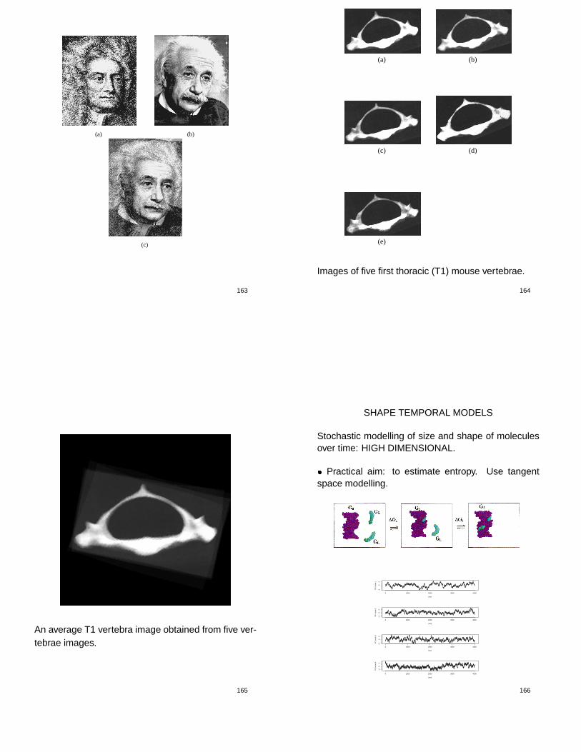
(a) (b)
(c)
163
(a) (b)
(c) (d)
(e)
Images of five first thoracic (T1) mouse vertebrae.
164
An average T1 vertebra image obtained from five ver-tebrae images.
165
SHAPE TEMPORAL MODELS
Stochastic modelling of size and shape of moleculesover time: HIGH DIMENSIONAL.� Practical aim: to estimate entropy. Use tangentspace modelling.
0 1000 2000 3000 4000
−3
02
time
PC
sco
re 1
0 1000 2000 3000 4000
−3
02
time
PC
sco
re 2
0 1000 2000 3000 4000
−3
02
time
PC
sco
re 3
0 1000 2000 3000 4000
−2
02
time
PC
sco
re 4
166
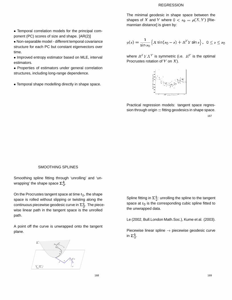
� Temporal correlation models for the principal com-ponent (PC) scores of size and shape. [AR(2)]� Non-separable model - different temporal covariancestructure for each PC but constant eigenvectors overtime.� Improved entropy estimator based on MLE, intervalestimators.� Properties of estimators under general correlationstructures, including long-range dependence.� Temporal shape modelling directly in shape space.
REGRESSION
The minimal geodesic in shape space between theshapes of
�and
*where > { ò S � ¹ � � 3 * � [Rie-
mannian distance] is given by:
� � ò � � ,� � � ò S } � � � � � ò S ' ò � o é - * � � � ò ~ 3 > y ò y ò Swhere é - * � - is symmetric (i.e. é - is the optimalProcrustes rotation of
*on
�).
Practical regression models: tangent space regres-sion through origin ¶ fitting geodesics in shape space.
167
SMOOTHING SPLINES
Smoothing spline fitting through ‘unrolling’ and ‘un-wrapping’ the shape space � �) .
On the Procrustes tangent space at time� S , the shape
space is rolled without slipping or twisting along thecontinuous piecewise geodesic curve in � �) . The piece-wise linear path in the tangent space is the unrolledpath.
A point off the curve is unwrapped onto the tangentplane.
α
αα
β* 1
2
1
2 Y
�(t)
*Y
β
α
� ��kΣ 2�� �
(t )0
*�(t)
Σk2
168
Spline fitting in � �) : unrolling the spline to the tangentspace at
� S is the corresponding cubic spline fitted tothe unwrapped data.
Le (2002, Bull.London Math.Soc.), Kume et al. (2003).
Piecewise linear spline � piecewise geodesic curvein � �) .
169

NONPARAMETRIC INFERENCE� The full Procrustes mean ÃØis a consistent estima-
tor of ‘extrinsic mean shape’ (Patrangenaru and Bhat-tacharya, 2003)� Central limit theorem for ÃØ
and a limiting� ) distribu-
tion for a pivotal test statistic � confidence regions.� Bootstrap confidence interval for mean shape basedon a pivotal statistic - NEEDS CARE in a non-Euclideanspace.� Coverage accuracy of bootstrap confidence region� � Ô ; ) � .� Bootstrap
�sample hypothesis test (not necessary
to have equal covariance matrices in each group).� Need to simulate from the null hypothesis of equalmean shapes, and so the individual samples are movedalong a geodesic to the pooled mean without chang-ing the inter-sample shape distances.� Simulation studies indicate accurate observed sig-nificance levels and good power.
170
DISCUSSION� At all stages geometrical information always avail-able� Statistical shape analysis of wide use in many disci-plines.� Great scope for further application in image analy-sis, e.g. medical imaging.� Non-landmark - curve - data
171
Selected References to papers:DG Kendall (1984,Bull.Lond.Math.Soc), Bookstein (1986,Sta-tistical Science), WS Kendall (1988,Adv.Appl.Probab.),DG Kendall (1989,Statistical Science), Mardia and Dry-den (1989, Adv.Appl. Probab; 1989, Biometrika), Dry-den and Mardia (1991, Adv.Appl,Probab) Dryden andMardia (1992, Biometrika) Goodall and Mardia (1993,Annals of Statistics), Le and DG Kendall (1993, An-nals of Statistics), Kent (1994, JRSS B), Le (1994,J.Appl.Probab.), Kent and Mardia (1997, JRSS B), Dry-den, Faghihi and Taylor (1997, JRSS B), WS Kendall(1998, Adv.Appl.Probab.), Mardia and Dryden (1999,JRSS B), Kent and Mardia (2001, Biometrika), Le (2002,Bull.London.Math.Society), Albert, Le and Small (2003,Biometrika).
172