Statistical Relational AI:

Logic, Probability and Computation

Kristian Kersting, Sriraam Natarajan, David Poolekristian.kersting@iais.fraunhofer.de,

snataraj@wfubmc.edu,poole@cs.ubc.ca

August 31, 2011

Abstract

One of the key challenges in building intelligent agents is closing thegap between logical and statistical AI, so that we can have rich representa-tions including objects, relations and uncertainty, that we can effectivelylearn and carry out inference with. Over the last 25 years there has beena considerable body of research into combinations of predicate logic andprobability forming what has become known as statistical relational artifi-cial intelligence (StaR-AI). We overview the foundations of the area, givesome research problems, proposed solutions, outstanding issues, and clearup some misconceptions that have arisen. We discuss representations, se-mantics, inference, learning and applications, and provide references tothe literature.

1 Introduction

Over the last 25 years there has been a considerable body of research intocombining first-order logic and probability, evolving into what has come to becalled statistical relational AI, which can be defined as:

the study and design of intelligent agents with imperfect sensors thatact in noisy worlds composed of objects, where there can be complexrelations among the objects.

This paper aims at reviewing the foundations of the area, motivating the issues,justifying some choices that have been made and giving some open problems.Laying bare the foundations will hopefully inspire others to join us in exploringthe frontiers and the yet unexplored areas.

One of the barriers to understanding this area is that it builds from multi-ple traditions, which often use the same vocabulary to mean different things.Common terms such as “variable”, “domain”, “relation”, and “parameter” have

1

Example Author Thread Length WhereRead UserActione1 known new long home skipse2 unknown new short work readse3 unknown follow up long work skipse4 known follow up long home skips. . . . . . . . . . . . . . . . . .

(a)

Individual Property Valuejoe likes resort 14joe dislikes resort 35. . . . . . . . .resort 14 type resortresort 14 near beach 18beach 18 type beachbeach 18 covered in wsws type sandws color white. . . . . . . . .

(b)

Figure 1: Two examples for datasets one can take advantage of to capturecharacteristics of interest of their unknown underlying probability distribution.

come to have accepted meanings in mathematics, computing, logic and prob-ability, but their meanings in each of these areas is different enough to causeconfusion.

Both predicate logic (e.g., the first-order predicate calculus) and Bayesianprobability can be seen as extending the propositional logic, one by adding re-lations, individuals and quantified variables, the other by allowing for measuresover possible worlds and conditional queries. Relational probabilistic models1,which form the basis of statistical relational AI, can be seen as combinations ofprobability and predicate calculus to allow for individuals and relations as wellas probabilities.

To understand the needs for such a combination, consider learning fromthe two datasets in Figure 1 (taken from [106]). Dataset (a) is the sort usedin traditional supervised and unsupervised machine learning and data mining.Standard textbook supervised learning algorithms can learn a decision tree, aneural network, or a support vector machine to predict UserAction. A beliefnetwork learning algorithm can be used to learn a representation of the distri-bution over all of the features. Dataset (b), from which we may want to predictwhat Joe likes, is different. Many of the values in the table are meaningless

1Here we use this term in the broad sense, meaning any models that combine relations andprobabilities.

2

names that can’t be used directly in supervised learning. Instead, it is the re-lationship among the individuals in the world that provides the generalizationsfrom which to learn. For example, we may want to learn that Joe likes resortsthat are near sandy beaches. Learning from such datasets has been studiedunder the umbrella of inductive logic programming [84, 74, 18] mainly becauselogic programs provide a good representation for the generalizations requiredto make predictions. Specifically, inductive logic programming (ILP) is a re-search field at the intersection of machine learning and logic programming. Itforms a formal framework for relational learning and has introduced practicalalgorithms for inductively learning relational descriptions (in the form of logicprograms) from examples and background knowledge. ILP is one of the foun-dations of StaR-AI, as it provides a toolbox of techniques for structure learningin relational domains.

One confusion about the area stems from the term “relational”; after all mostexisting datasets are, or can be, stored in relational databases. The techniquesof relational probabilistic models are applicable to cases where the values in thedatabase are names of individuals, and it is the properties of the individuals andthe relationship between the individuals that are modeled. It is sometimes alsocalled multi-relational learning, as it is the interrelations that are important.This is a misnomer because, as can be seen in Figure 1 (b), it is not multiplerelations that cause problems (and provide opportunities to exploit structure),as a single triple relation can store any relational database (in a so-called triple-store).

The term statistical relational AI comes from not only having probabilitiesand relations, but that the models are derived from data and prior knowledge.

2 Motivation

Artificial intelligence (AI) is the study of computational agents that act intel-ligently [106, 115]. The basic argument for probability as a foundation of AIis that agents that act under uncertainty are gambling, and probability is thecalculus of gambling in that agents who don’t use probability will lose to thosethat do use it [130]. While there are a number of interpretations of proba-bility, the most suitable is a Bayesian or subjective view of probability: ouragents do not encounter generic events, but have to make decisions in particularcircumstances, and only have access to their percepts and their beliefs.

In probability theory, possible worlds are described in terms of so-calledrandom variables (although they are neither random nor variable). A randomvariable has a value in every world. We can either define random variablesin terms of worlds or define worlds in terms of random variables. A randomvariable having a particular value is a proposition. Probability is defined interms of a non-negative measure over sets of possible worlds that follow somevery intuitive axioms.

In Bayesian probability, we make explicit assumptions and the conclusionsare logical consequences of the specified knowledge and assumptions. One par-

3

ticular explicit assumption is the assumption of conditional independence. ABayesian network [93] is an acyclic directed graphical model of probabilistic de-pendence where the nodes are random variables. A Bayesian network encapsu-lates the independence: a variable is conditionally independent of other variablesthat are not its descendants in the graph given its parents in the graph. Thishas turned out to be a very useful assumption in practice. Undirected graphicalmodels [93] encapsulate the assumption that a variable is independent of othervariables given its neighbours.

These motivations for probability (and similar motivations for utility) do notdepend on non-relational representations. We also want to be able to reasonabout individuals2 and relationships among individuals. In statistical relationalAI, we want to condition on properties of individuals and relations among indi-viduals and make probabilistic predictions about properties and relationships.We often want to build the models before we know which individuals exist in adomain, so that the models can be applied to diverse populations.

The key property that is exploited is that of exchangeability: those individ-uals about which we have the same information should be treated identically.Formally, this means we can exchange the names, and still get the same proba-bilities. This implies that before we know anything particular about any of theindividuals, they all should share their probabilistic parameters. Results fromStatistics, particularly the celebrated De Finetti’s theorem [17, 54], motivatethe forms of possible models (if we allow the population to be unbounded).

3 Representation

Statistical relational models are typically defined in terms of parameterizedrandom variables [101] which are often drawn in terms of plates [7]. A parame-terized random variable corresponds to a predicate (atom) or a function symbolin logic. It can include logical variables (which form the parameters). In thefollowing examples, we will write logical variables (which denote individuals) inupper case, and constants, function and predicate symbols in lower case. Weassume that the logical variables are typed, where the domain of the type, theset of individuals of the type, is called the population.

Parameterized random variables are best described in terms of an example.Consider the case of diagnosing students’ performance in adding multi-digitnumbers of the form

x1 x0+ y1 y0

z2 z1 z0

2Individuals are things. They are also called “objects”, but that terminology is oftenconfusing to people who have been brought up with object-oriented programming, whereobjects are data structures and associated methods. For example, a person individual is areal person and not a data structure that encapsulates information about a person. We canbe uncertain about the properties of a person, but a computer is not uncertain about its datastructures.

4

x(D,P)

y(D,P) z(D,P,S,T)

c(D,P,S,T)

knows_carry(S,T) knows_add(S,T)

D,P

S,T

Figure 2: Belief network with plates for multidigit addition

S

gr(S,C)

i(S) d(C)

C

Figure 3: Plate representation of the grades model

A student, given values for the x ’s and the y ’s, provides values for the z ’s.The aim is to determine whether the students have mastered addition fromobservations of their performance.

Whether a student gets the correct answer for zi depends on xi , yi , thevalue carried in and whether she knows addition. Whether a student gets thecorrect carry depends on the previous x , y and carry, and whether she knownshow to carry. This dependency can be seen in Figure 2. Here x (D ,P) is aparameterized random variable. There is a random variable for each digit Dand each problem P . A ground instance, such as x (d3, problem57), is a randomvariable that may represent the third digit of problem 57. Similarly, there is a z -variable for each digit D , problem P , student S , and time T . The plate notationcan be read as duplicating the random variable for each tuple of individual theplate is parameterized by.

As another example, Figure 3 gives a plate representation of a model to pre-dict the grades of students in courses. In this figure, S is a logical variable thatdenotes a student and C is a logical variable that denotes a course. Parameter-ized random variable gr(S ,C ) denotes the grade of S in course C , parameterizedrandom variable i(S ) denotes the intelligence of student S , and d(C ) representsthe difficulty of course C . Note that this figure redundantly includes the log-ical variables in the plates as well as arguments to the parameterized randomvariables.

Such parametrized models represent their grounding, where there is an in-stance of each random variable for each assignment of an individual to a logical

5

gr(s,c1)

i(s)

i(c)

i(k) gr(c,c1)

gr(k,c1)

gr(s,c2)

gr(c,c2)

gr(k,c2)

d(c1) d(c2)

Figure 4: Grounding of the grades model for 3 people and 2 courses

S

gr(S,C)

i(S) d(C)

C

θg

θdθi

Figure 5: Plate representation of the grades model, with shared parametersexplicit

variable. Figure 4 shows such a grounding where there are three students Sam(s), Chris (c) and Kim (k) and two courses (c1 and c2).

For the plate model of Figure 3 with n students and m courses, there are nminstance of the grade random variable, n instances of the intelligence randomvariable and m instance of the difficulty random variable. Thus there are nm +n + m random variables in the grounding.

Note the independence assumptions in this example: The intelligence of thestudents are independent of each other give no observations. The difficulty ofthe courses are independent of each other, given no observations. The gradesare independent given the intelligence and the difficulty. Given no observations,the grades are dependent on each other. Given observations on grades, the intel-ligence variables and the difficulty variables can be completely interdependent.

While we have given directed models here, the same principles also apply toundirected models. The basic principle used by all methods is that of parametersharing : the instances of the parameterized random variables created by sub-stituting constants for logical variables share the same probabilistic parameters.The various languages differ in how to specify the conditional probabilities ofthe parametrized random variables given their parents, or the other parametersof the probabilistic model. Often in plate models [7, 52], the numerical parame-ters are made explicit, to emphasize that the parameters do not depend on theindividuals.

6

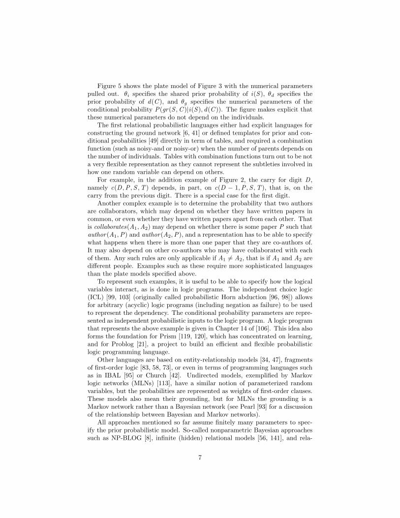
Figure 5 shows the plate model of Figure 3 with the numerical parameterspulled out. θi specifies the shared prior probability of i(S ), θd specifies theprior probability of d(C ), and θg specifies the numerical parameters of theconditional probability P(gr(S ,C )|i(S ), d(C )). The figure makes explicit thatthese numerical parameters do not depend on the individuals.

The first relational probabilistic languages either had explicit languages forconstructing the ground network [6, 41] or defined templates for prior and con-ditional probabilities [49] directly in term of tables, and required a combinationfunction (such as noisy-and or noisy-or) when the number of parents depends onthe number of individuals. Tables with combination functions turn out to be nota very flexible representation as they cannot represent the subtleties involved inhow one random variable can depend on others.

For example, in the addition example of Figure 2, the carry for digit D ,namely c(D ,P ,S ,T ) depends, in part, on c(D − 1,P ,S ,T ), that is, on thecarry from the previous digit. There is a special case for the first digit.

Another complex example is to determine the probability that two authorsare collaborators, which may depend on whether they have written papers incommon, or even whether they have written papers apart from each other. Thatis collaborates(A1,A2) may depend on whether there is some paper P such thatauthor(A1,P) and author(A2,P), and a representation has to be able to specifywhat happens when there is more than one paper that they are co-authors of.It may also depend on other co-authors who may have collaborated with eachof them. Any such rules are only applicable if A1 6= A2, that is if A1 and A2 aredifferent people. Examples such as these require more sophisticated languagesthan the plate models specified above.

To represent such examples, it is useful to be able to specify how the logicalvariables interact, as is done in logic programs. The independent choice logic(ICL) [99, 103] (originally called probabilistic Horn abduction [96, 98]) allowsfor arbitrary (acyclic) logic programs (including negation as failure) to be usedto represent the dependency. The conditional probability parameters are repre-sented as independent probabilistic inputs to the logic program. A logic programthat represents the above example is given in Chapter 14 of [106]. This idea alsoforms the foundation for Prism [119, 120], which has concentrated on learning,and for Problog [21], a project to build an efficient and flexible probabilisticlogic programming language.

Other languages are based on entity-relationship models [34, 47], fragmentsof first-order logic [83, 58, 73], or even in terms of programming languages suchas in IBAL [95] or Church [42]. Undirected models, exemplified by Markovlogic networks (MLNs) [113], have a similar notion of parameterized randomvariables, but the probabilities are represented as weights of first-order clauses.These models also mean their grounding, but for MLNs the grounding is aMarkov network rather than a Bayesian network (see Pearl [93] for a discussionof the relationship between Bayesian and Markov networks).

All approaches mentioned so far assume finitely many parameters to spec-ify the prior probabilistic model. So-called nonparametric Bayesian approachessuch as NP-BLOG [8], infinite (hidden) relational models [56, 141], and rela-

7

tional Gaussian processes [14, 144, 143, 127] allow for infinitely many param-eters, for example because there could be an unbounded number of classes ofindividuals (or parametrized random variables with an unbounded range). Ascomputers can only handle finite representations, these models require someprocess to specify how these parameters are generated.

4 Representational Issues

Many probabilistic relational representation languages already exists; see e.g. [19,38, 22] for overviews. Rather than listing and describing the properties of thevarious proposal, we here descrive some issues that arise in designing represen-tation language.

4.1 Desiderata of a Representation Language

Often a good representation is a compromise between many competing objec-tives. Some of the objectives of a representation language, include:

prediction accuracy: is it able to generalize to predict unseen examples?Thus the representation should be able to represent the generalized knowl-edge of the domain.

compactness: is the representation of the knowledge succinct? This is relatedto prediction accuracy, as it is conjectured that a compact representationwill be best able to generalize. It is also related to introducing latentrandom variables, as the reason that we introduce latent variables is tomake a model simpler.

expressivity: is it rich enough to represent the knowledge required to solve theproblems required of it? Can it deal with discrete and continuous randomvariables? Can it deal with domains evolving over time?

efficient inference: can it to solve all/average/some problems efficiently? Canit efficiently deal with latent variables?

understandability: can someone understand what has been learned?

modularity : can parts of the representation be understood or learned sepa-rately? This has two aspects:

• the ability to conjoin models that are developed independently. Ifdifferent teams work on individual parts of a model, can these partseasily be combined? This should be able to be done even if the teamsdo not know their work will be combined and even if the teams havedeveloped both directed and undirected models.

• the ability to decompose a model into smaller parts for specific ap-plications. If there is a big model, can someone take a subset of the

8

model and use it? Can someone take advantage of a hierarchicaldecomposition into weakly interacting parts?

ability to incorporate prior knowledge: if there is domain knowledge thathas been acquired in a research community, can it be incorporated intothe model?

interoperability with data: can it learn from multiple heterogeneous datasets? Heterogeneous can mean having different overlapping concepts, de-rived from different contexts, at different levels of abstraction (in termsof generality and specificity) or different levels of detail (in terms of partsand subparts). It should also be able to incorporate causal data thathas arisen from interventions and observational data that only involvedpassively observing the world.

latent factors: can it learn the relationship between random variables if therelationship is a function of observed and unobserved (latent) characteris-tics, potentially in addition to contextual factors? Can it even introducelatent factors on the fly?

The promise of statistical relational AI is to automate decisions in com-plex domains. For complex domains, there are many diverse relevant pieces ofinformation that cannot be ignored. For a system to be relied on for critical life-or-death decisions or ones that rely on large economic risks, the system needsto be able to explain or at least justify its recommendations to the people whoare legally responsible, and these recommendations need to be based on thebest available evidence (and preferably on all available evidence that is possiblyrelevant). Of course, not all of the existing representations have attempted toachieve all of these desiderata.

Sections 4.2-4.6 present some issues that have arisen in the various represen-tations. Whether these turn out to be unimportant or whether one choice willprevail is still an open question.

4.2 Directed versus undirected models

In a manner similar to the difference between Bayesian networks and Markovnetworks [93], there are directed relational models (e.g., [99, 103, 47, 73]) andundirected models (e.g., [131, 113, 44, 138]). The main differences between theseare:

• The probabilities of the directed models can be directly interpreted asconditional probabilities. This means that they can be explained to users,and can be locally learned if all of the relevant properties are observed.

• Because the probabilities can be interpreted locally, the directed repre-sentations are modular. The probabilities can be acquired modularly, andneed not change if the model is expanded or combined with another model.

9

• For inference in directed models, typically only a very small part of thegrounded network needs to be used for inference. In particular, only theancestors of the observed and query relations need to be considered. Thishas been characterized as abduction [97], where the relevant probabilitiescan be extracted from proofs (in the logical sense) of the observations andqueries.

• The directed models require the structure of the conditional probabili-ties to be acyclic. (A specification of P(A|B) and P(B |A) is typicallyinconsistent, and sometimes does not specify a unique distribution.) Forrelational models, this is problematic if we have conditional probabilitiesof the form:

P(foo(X )|foo(Y ) . . . )

To make this acyclic, we could totally order the individuals, and enforcea “less than” operation. However, this means that the individuals are nolonger exchangeable. One example where this arises is if we wanted tospecify the probability that friendship is transitive:

P(friends(X ,Y )|∃Z friends(X ,Z ), friends(Z ,Y ))

Naive ways to incorporate such rules do not work as expected.

Undirected models, such as Markov logic networks [113], do not have a problemwith acyclicity, but the weights of the undirected models cannot directly inter-preted as probabilities, and it is often very difficult to interpret the numbersat all. However, as many of the applications where we may want to predictrelations have a relation on some individual depending on relations on otherindividuals, the undirected models tend to be more effective for these domains.

It is an open research question to allow directed models to handle cyclicdependencies and to allow the undirected models to be modular and explainable.

4.3 Factors and Clauses

In graphical models, the next highest level of data structure is the factor orpotential [125, 146, 33]. Factors represent functions from the domains of sets ofvariables into other values (typically reals). For example, a factor on randomvariables {A,B ,C} is a function from dom(A)×dom(B)×dom(C )→ <, wheredom(A) is the domain of random variable A, and < is the set of real numbers.Factors can represent conditional probabilities, utilities, arbitrary potentials,and the intermediate results of computation. An alternative to using an explicitrepresentation of full factors is to represent the value of one assignment tovariables, or to any Boolean function of assignments to values, such as usingclauses [15]; this enables local structure to be exploited including context-specificindependence and zero parameters [9, 116].

In relational representations the corresponding representation is a parame-terized factor or parfactor [101], which is a triple

〈C ,V , t〉

10

where C is a set of inequality constraints on logical variables, V is a set ofparameterized random variables and t is a factor on V . Note that t will be thefactor that is used for all assignments of individuals to logical variables in V . Ifthe factor represents a clause, the table specifies just a single number, and thenV is written as a first-order clause as for example done in MLNs.

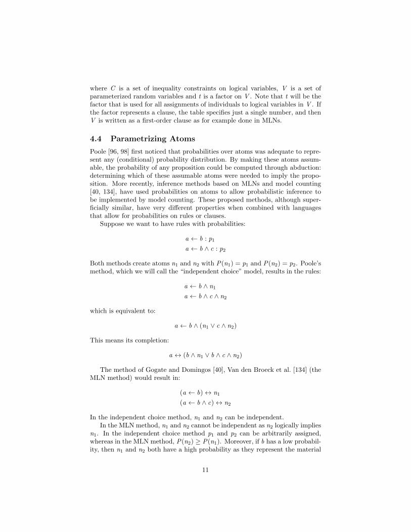
4.4 Parametrizing Atoms

Poole [96, 98] first noticed that probabilities over atoms was adequate to repre-sent any (conditional) probability distribution. By making these atoms assum-able, the probability of any proposition could be computed through abduction:determining which of these assumable atoms were needed to imply the propo-sition. More recently, inference methods based on MLNs and model counting[40, 134], have used probabilities on atoms to allow probabilistic inference tobe implemented by model counting. These proposed methods, although super-ficially similar, have very different properties when combined with languagesthat allow for probabilities on rules or clauses.

Suppose we want to have rules with probabilities:

a ← b : p1

a ← b ∧ c : p2

Both methods create atoms n1 and n2 with P(n1) = p1 and P(n2) = p2. Poole’smethod, which we will call the “independent choice” model, results in the rules:

a ← b ∧ n1

a ← b ∧ c ∧ n2

which is equivalent to:

a ← b ∧ (n1 ∨ c ∧ n2)

This means its completion:

a ↔ (b ∧ n1 ∨ b ∧ c ∧ n2)

The method of Gogate and Domingos [40], Van den Broeck et al. [134] (theMLN method) would result in:

(a ← b)↔ n1

(a ← b ∧ c)↔ n2

In the independent choice method, n1 and n2 can be independent.In the MLN method, n1 and n2 cannot be independent as n2 logically implies

n1. In the independent choice method p1 and p2 can be arbitrarily assigned,whereas in the MLN method, P(n2) ≥ P(n1). Moreover, if b has a low probabil-ity, then n1 and n2 both have a high probability as they represent the material

11

implication which is true whenever b is false. As such, in the MLN method, p1

and p2 are close to each other when b has a low probability. However, in the in-dependent choice method, they represent conditional probabilities and can havearbitrary probabilities. Sato [119, 120] has done extensive work on learning forthe independent choice case.

What seems to be a slight different in the reading of rules has a big effecton the semantics. The independent choice method allows a simple semanticsin terms of independent atomic choices and a logic program that gives theconsequences of the choices [98, 99]. The semantics of Gogate and Domingos[40], Van den Broeck et al. [134] does not assume independent atoms, but appealsto the maximum entropy assignment, which makes it much more difficult tointerpret the numbers.

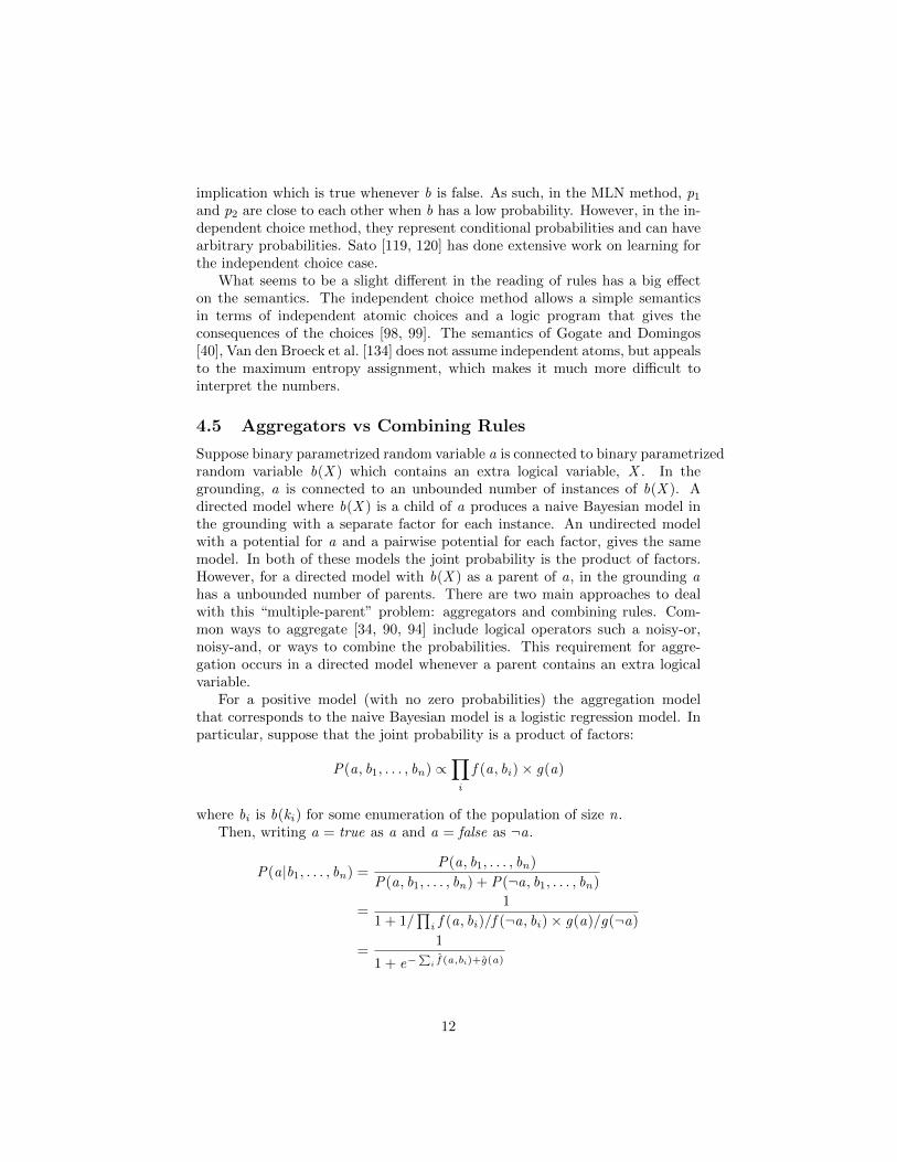
4.5 Aggregators vs Combining Rules

Suppose binary parametrized random variable a is connected to binary parametrizedrandom variable b(X ) which contains an extra logical variable, X . In thegrounding, a is connected to an unbounded number of instances of b(X ). Adirected model where b(X ) is a child of a produces a naive Bayesian model inthe grounding with a separate factor for each instance. An undirected modelwith a potential for a and a pairwise potential for each factor, gives the samemodel. In both of these models the joint probability is the product of factors.However, for a directed model with b(X ) as a parent of a, in the grounding ahas a unbounded number of parents. There are two main approaches to dealwith this “multiple-parent” problem: aggregators and combining rules. Com-mon ways to aggregate [34, 90, 94] include logical operators such a noisy-or,noisy-and, or ways to combine the probabilities. This requirement for aggre-gation occurs in a directed model whenever a parent contains an extra logicalvariable.

For a positive model (with no zero probabilities) the aggregation modelthat corresponds to the naive Bayesian model is a logistic regression model. Inparticular, suppose that the joint probability is a product of factors:

P(a, b1, . . . , bn) ∝∏i

f (a, bi)× g(a)

where bi is b(ki) for some enumeration of the population of size n.Then, writing a = true as a and a = false as ¬a.

P(a|b1, . . . , bn) =P(a, b1, . . . , bn)

P(a, b1, . . . , bn) + P(¬a, b1, . . . , bn)

=1

1 + 1/∏

i f (a, bi)/f (¬a, bi)× g(a)/g(¬a)

=1

1 + e−∑

i f (a,bi )+g(a)

12

where f (a, bi) = log(f (a, bi)/f (¬a, bi)) and g(a) = log g(a)/g(¬a). We can

then represent f (a, bi) as wbi and ˆg(a) as w ′ (as a is fixed). In a standardgraphical model, n is fixed and it does not matter how the values of bi arerepresented. However, in a relational model where n can vary, the details of therepresentation affect how the model changes with n.

For example, suppose we have a logistic regression model that represents: ais true if and only if b is true for more than 5 individuals out of a population of10. Now consider what this model predicts when the population size is 20. If thevalues of b are represented with 0 = false and 1 = true, this model will have atrue if b is true for more than 5 individuals out of a population of 20. However,if the values of b are represented with −1 = false and 1 = true, this model willhave a true if b is true for more than 10 individuals out of a population of 20.If the values of b are represented with 1 = false and 0 = true, this model willhave a true if b is true for more than 15 individuals out of a population of 20.Different choices can result in arbitrary thresholds for the population.

While the dependence on population may be arbitrary when a single pop-ulation is observed, it affects the ability of a model to predict when multiplepopulations are observed. For example, suppose we want to model whethersomeone is happy depends on the number of their friends that are mean tothem. One model could be that people are happy as long as they have morethan 5 friends who are not mean to them. Another model could be that peopleare happy if more than half of their friends are not mean to them. A third modelcould be that people are happy as long as fewer than 5 of their friends are meanto them. These three models coincide for people with 10 friends, but makedifferent predictions for people with 20 friends. A particular logistic regressionmodel (or a naive Bayesian model) is only able to model one of the dependenciesof how predictions depend on population, and so cannot properly fit data thatdoes not adhere to that dependence. One way to fit various dependencies is toalways include the property 1 which has the value 1 for each individual (in thenaive Bayesian model, this needs to be observed). Another, as typically usedin Markov logic networks, is to have separate parameters for the positive andnegative cases. Each of these can model linear dependence on population.

While aggregators assume that the parents of a random variable “collec-tively” influence the target, combining rules [50, 86, 58] take the opposite viewi.e., they assume “independence of causal influence,” (ICI) in that each parentof a random variable influences the target independently. This is to say that,combining rules capture the notion of causal independence [46] in directed mod-els. In this view, multiple causes on a target variable can be decomposed intoseveral independent causes whose effects are combined to yield a final value.Each parent or set of related parents produces a different value for the childvariable, all of which are combined using a deterministic or stochastic function.Depending on how the causes are decomposed and how the effects are combined,we can express the conditional distribution of the target variable given all thecauses as a function of the conditional distributions of the target variable giveneach independent cause using a combining rule. When analyzing the difference

13

between directed vs undirected models, it is important to understand how torepresent causal independencies in undirected models. A first-step in this direc-tion has been taken by Natarajan et al. [87] where an algorithm for converting adirected model with combining rules to an equivalent MLN has been presented.

For a particular class of combining rules called decomposable combining rules,it can be shown that there is an equivalent class of aggregators. Learningin the presence of combining rules have been considered previously [50, 86]where the EM-based algorithms use the value-based aggregation functions. Ata fairly high level, decomposable combining rules are functions that yield thesame target distribution irrespective of the order of the parents. The mostcommon ones used in the literature are mean, weighted mean and noisy-orcombining rules [86, 50, 58]. For these combining rules there are equivalentaggregators. For example, mean can be represented as a stochastic choice usingan uniform distribution over the parent values, weighted mean corresponds to astochastic choice given the weight distribution while noisy-or has a value-basedinterpretation [93] and a distribution based interpretation [86]. On the otherhand, for an arbitrary combining rule, determining an equivalent aggregator isstill an open question.

4.6 Probability-Specificity Tradeoff

It is often not clear whether highly complex but specific logical structures withextreme probabilities (close to 0 or 1) or simpler but less-specific logical struc-tures with arbitrary distributions form better models. In many domains suchas medical domains, using specific rules with probabilities close to 0 or 1 allowsfor easy interpretation. In such cases, the more “probabilistic” a rule becomes,the harder it is to interpret. On the other hand, from an inference perspec-tive, algorithms based on sampling and belief propagation perform better if therules are not nearly deterministic. Similar to the classic “bias-variance” trade-off in machine learning, there seems to be a probability-specificity tradeoff inprobabilistic logic methods.

If prediction accuracy were the only criterion for preference of models, whethermore specific and hence deterministic or more probabilistic models is better de-pends on the loss function. In terms of Ockham’s razor of preferring simplermodels, it isn’t clear how to trade off the complexity of deterministic ruleswith stochastic predictions, as we usually do not use the optimal information-theoretic encoding for probabilities or for the structure.

5 Inference

Inference in probabilistic relational models refers to computing the posteriordistribution of some variables given some evidence.

A standard way to carry out inference in such models is to try to generateand ground as few of the parameterized random variables as possible. E.g., inthe ICL, the relevant ground instances can be carried out using abduction [97].

14

Lifted Inference

Graph based

Exact[101, 25, 82, 65]

[66, 11, 123, 24, 13]

Approximate

DeterministicApproximation

[128, 57, 124, 62][114, 88, 45, 1]

Sampling[81, 109, 145]

Interval[23]

PreProcessing[126, 79]

Search[39, 40, 51, 134]

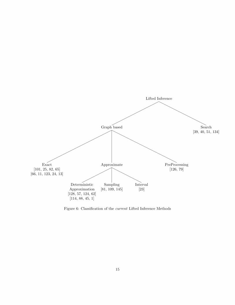
Figure 6: Classification of the current Lifted Inference Methods

15

Figure 7: Lifted Inference Example. (a) Parfactor consists of two predicates aand b. (b) The case when summing out b. All ground instances of b can begrouped together. (c) The case when eliminating a. All ground instances of bare now connected.

More recently, there has been work on lifted probabilistic inference [101,25, 128, 82], where the idea is to carry out probabilistic reasoning at the liftedlevel, without grounding out the parameterized random variables. Instead, wecount how many of the probabilities we need, and when we need to multiplya number of identical probabilities, we can take the probability to the powerof the number of individuals. Lifted inference turns out to be a very difficultproblem, as the possible interactions between parameterized random variablescan be very complicated. Nevertheless, there is already substantial work onlifted inference.

A taxonomy of lifted inference methods is presented in Figure 6. At a fairlyhigh-level, lifted inference algorithms can be understood as being inspired bygraphical models (shown as graph based in the Figure) or by logical approaches(shown as search based). It should be mentioned that graph vs search basedclassification is orthogonal to exact vs approximate classification. But, since thesearch based methods [39, 40, 51, 134] are more recent and fewer in number, wegrouped them as a separate class and focus in this section mainly on the graphbased methods. The graph based methods can be divided into exact inferencemethods (which are based on variable elimination), approximate methods andmethods for pre-processing the data.

To understand the exact inference methods, consider a simple parfactor on〈{}, {a, b(X )}, t〉, where the population of X has size n (see Figure 7(a)). Whensumming out all instances of b(X ) (as shown in Figure 7 (b)), we can note thatall of the factors in the grounding have the same value and so can be takento the power of n, which can be done in time logarithmic in n [101], whereasthe grounding is linear in n. This operation invented by Poole [101] was calledinversion elimination by de Salvo Braz et al. [25]. However, if we were to sumout a instead (as in Figure 7 (c)), in the resulting grounding all instances of

16

Figure 8: Illustration of lifted BP algorithm. From left to right, the stepsof the lifted inference algorithm taken to compress the factor graph assumingno evidence. The shaded/colored small circles and squares denote the groupsand signatures produced running the algorithm. On the right-hand side, theresulting compressed factor graph is shown. On this network a modified BPalgorithm is ran.

b(X ) are connected, and so there would be a factor that is of size exponential inn. de Salvo Braz et al. [25] showed how, rather than representing the resultingfactor, we only need to the count of the number of instances of b(X ) whichhave a certain value, and so the subsequent elimination of b(X ) can be done intime polynomial in n (this is linear in n if b(X ) is binary, and if b(X ) has kvalues, the time is O(nk−1)). Milch et al. [82] proposed counting formulae as arepresentation of the intermediate lifted formulae. All of these algorithms needto ground a population in certain circumstances.

In a distinct yet related work, Sen et al. [123] propose the idea of liftedvariable elimination where computational trees are used to group together in-distinguishable individuals. These indistinguishable individuals are determinedby identifying shared factors (i.e., factors that compute the same function andhave the same input and output values). This idea was later extended by thesame group to approximate inference [124]. Choi et al. [13] addressed the prob-lem of lifted inference in continuous domains. Their approach assumes that themodel consists of Gaussian potentials. Their algorithm marginalizes variablesby integrating out random variables using inversion elimination operation. Ifthe elimination is not possible, they consider elimination of pairwise potentialsand the marginals that are not in pairwise form are converted to pairwise formand then eliminated.

The approximate methods can be further classified into deterministic approx-imation methods that are based on variational methods such as belief propa-gation, sampling based methods, and interval methods. The deterministic ap-proximate methods group random variables and factors in to sets if they haveidentical message passing computation trees [128, 57, 62]. Consider the factorgraph presented in Figure 8 with three nodes A, B and C sending identicalmessages to the neighbors. As can be seen from the figure, since nodes A and Csend and receive the same message, they can be clustered together. B cannot

17

be grouped with A or C since it sends twice the same message and hence isconsidered to be different from the other two. The resulting compressed graphis shown in the end. These methods have been successfully applied to severaldifferent problems and extended in several ways [88, 62, 45, 1].

There are sampling methods developed based on MCMC for certain for-malisms such as MLNs [109] and BLOG [81]. Zettlemoyer et al. [145] ex-tended particle filters to logical setting. Braz et al. [23] proposed a methodthat starts from the query, propagates intervals instead of point estimates andincrementally grounds the lifted network. Lastly, there are some methods forpre-processing [126, 79] that reduce the network size drastically so that groundinference can be performed efficiently on the reduced network.

The search based methods form the dual to the graph-based methods inanalogy to how variable elimination is the dynamic programming variant ofsearch-based recursive conditioning [16]. The method by Gogate and Domin-gos [40] reduce the problem of lifted probabilistic inference to weighted modelcounting in a lifted graph. Another recent approach to lifted inference compilesthe lifted graph into a weighted CNF and then runs weighted model counting onthe compiled network [134]. Both these approaches were developed in paralleland have promising potential to lifted inference.

Lifted inference has come a long way since Poole’s lifted variable eliminationand is currently a very active area of research inside Statistical Relational AIas can be evidenced by a surge in the number of algorithms and applications inthe last few years. For instance, belief propagation based methods have beensuccessfully applied to model counting [57], social networks [62] and contentdistribution problems [62]. Nath and Domingos used an approximate version ofLifted Belief Propagation for video segmentation [88]. Ahmadi et al. [1] appliedthe lifted evidence message passing to problems such as PageRank and KalmanFilters. In a related work, Choi et al. [12] developed Relational Gaussian Modelsto model large dynamic systems and developed an exact inference for LiftedKalman filters. Sen et al.’s [123, 124] lifted variable elimination has been usedfor efficient inference in probabilistic data bases. Other applications of liftedinference techniques include information extraction and retrieval, semantic rolelabeling, citation matching and entity resolution [81, 109, 128, 126, 114, 89, 40].Lifted inference in continuous models have been applied to market analysis [13].

6 Learning

Consider a single relation, that records the grade for students in courses3:

3In a real dataset, each student would be identified by unique (meaningless) identifier, suchas a student number. Similarly a course would also have a unique identifier, and there wouldbe some way to get the information about the department, number, and term taken. In a realdatabase there would be much more information about each course and each student.

18

Student Course GradeSam cs245 85Chris cs222 55Sam cs222 76Chris cs333 65. . . . . . . . .

The aim might be to predict how Sam would do on another course, say cs333.This problem has been studied in terms of reference classes [111], where it hasbeen advocated to use the narrowest reference class for which there are adequatestatistics [69]. Here that might mean to use the grade of Sam, the average gradein the course cs333 or some mix of all reference classes. Suppose that the averagegrade of all students in all courses was 65, and that the average grade of Samwas 80 and the average grade of cs333 was also 80. One might think to predictsomewhere between 65 and 80, as that is the range of the statistics available.However, it is likely that Sam will get a higher grade than 80; after all Sam isa well-above-average student and cs333 is an easy course4.

In the simplest case, we have a model such as in Figure 3, where all ofthe relations have been observed. In such cases, parameter sharing can lead tolearning conditional probabilities by counting or by adapting supervised learningtechniques [119, 34, 61]. For example, the maximum likelihood value for theshared parameter P(gr(S ,C ) = a|i(S ) = high, d(C ) = low) could be the ratioof counts

|{〈S ,C 〉 : gr(S ,C ) = a, i(S ) = high, d(C ) = low}||{〈S ,C 〉 : i(S ) = high, d(C ) = low}|

.

This produces the probability that a randomly chosen student-course pair witha highly intelligent student and a low difficulty course, will have an “a” grade.This will typically produce a low probability in a large data base, as moststudents have not taken most courses. This might be what is wanted. If however,we want to predict how a intelligent student would do on an easy course, weshould only consider the courses students have taken, and then the maximumlikelihood value for P(gr(S ,C ) = a|i(S ) = high, d(C ) = low) would be theratio:

|{〈S ,C 〉 : gr(S ,C ) = a, i(S ) = high, d(C ) = low}||{〈S ,C 〉 : i(S ) = high, d(C ) = low ,∃G gr(S ,C ) = G}|

.

Typically, however, we don’t directly observe the difficulty of courses and theintelligence of students. A more sophisticated way to model such predictionsis in terms of latent (hidden or unobserved) variables. For example, one couldadopt the model of Figure 3, but where i(S ) and d(C ) are latent variables. Ofcourse, when these are unobserved variables, it may not be the intelligence ofthe students and the difficulty of the courses that are discovered by the learning;a learner will discover whichever categorizations best predict the observations.Note that inducing properties of individuals is equivalent to a (soft) clustering

4It could also be the case that the average for cs333 is high because cs333 is only taken bythe top students. We would also like the learning system to discover this.

19

of the individuals. For example, if there are three values for i(S ), assigninga value to i(s) for each student s is equivalent to assigning s to one of threeclusters. The use of latent variables allows for much greater modelling than canbe done with reference classes [10].

Although the difficulty of the courses and the intelligence of the students area priori independent, they become dependent once some grades are observed.For example, if students s and c have taken a course in common (and thedifficulty of the course is not observed), i(s) and i(c) are dependent, and if cand k have also taken another course in common, all three random variables areinterdependent. Thus inference in these models quickly becomes intractable.Since inference is a key step in learning (for computing the expected counts5)learning such models is intractable.

Next to estimating the parameter from data, we may also select the modelstructure, i.e., a set of parameterized factors from data [119, 35, 20, 67]. This canbe viewed as adapting traditional inductive logic programming (ILP) techniquesto take uncertainty explicitly into account. Whereas ILP typically employs some0− 1 score to evaluate hypotheses (the number of correctly covered examples),learning probabilistic relational models employs some probabilistic score suchas (pseudo) likelihood (the likelihood of correctly covering the examples).

With this in mind, the vanilla structure learning algorithm for probabilis-tic relational models might be sketched as a greedy hill-climbing search algo-rithm [20, 22]. Assuming some data given, we take some initial theory T0, saygr , i , and d are not inter-connect by any edges, as starting point and computethe parameters maximizing some score such as the (pseudo) likelihood. Then,we use so-called refinement operators to compute neighbours of T0. A refine-ment operator takes the current theory, makes small, syntactic modifications toit, and returns a copy of the modified theory. Whereas for Bayesian networks,typical refinements are adding, deleting, or flipping single edges, for relationalmodels, we instead add or delete single literals to formulas, negate them, or in-stantiate respectively unify variables in them. For instance we may hypothesisethat the grade gr(S ,C ) of student S in course C depends on the intelligencei(S ) of the student S . This essentially corresponds to adding, deleting, or flip-ping multiple edges in the underlying ground graphical model. In our case, weadd an edge for each student S and course C pair. Now, if the score for one ofthe neighbours, say H , is larger then the currently best theory T0, we take Has new current best theory T1 and iterate. The process is continued until nofurther improvements in score are obtained.

Recently, there have been some advances to this vanilla learning approach,especially in the case of Markov Logic networks. For instance, we may view agiven set of examples (a relational database) as a hypergraph. A hypergraph is astraightforward generalization of a graph, in which an edge can link any number

5In the presence of missing data or latent factors, the maximum likelihood estimate typi-cally cannot be written in closed form. It is a numerical optimization problem, and all wellknown algorithms such as the Expectation-Maximization (EM) algorithm or gradient-basedmethods involve nonlinear, iterative optimization and multiple calls to inference for computingthe expected counts.

20

of nodes, rather than just two. Now, the constants appearing in an example arethe nodes and ground atoms are the hyperedges. Each hyperedge is labeled withthe predicate symbol of the corresponding ground atom. Nodes (constants) arelinked by a hyperedge if and only if they appear as arguments in the hyperedge.Now, any path of hyperedges can be generalized into conjunctions of relationalatoms by variablizing their arguments. Mihalkova and Mooney [78] as well asKok and Domingos [68] proposed to use relational path finding [112] for learningMarkov logic networks. Each path is turned into a set of conjunctions of atomsfor which we estimate the weights.

Another recent advance is triggered by the insight that finding many roughrules of thumb of how to change probabilistic models locally can be a lot easierthan finding a single, highly accurate model. For relational dependency net-works, for example, one can represent the conditional probability distributionassociated with each predicate as a weighted sum of regression models grown ina stage-wise optimization using gradient boosting [85]. This functional gradientapproach has also successfully been used to train conditional random fields forlabeling relational sequences [44] and to learn relational policies [60]. The ben-efits of a boosted learning approach are manifold. First, being a nonparametricapproach the number of parameters grows with the number of training episodes.In turn, interactions among random variables are introduced only as needed, sothat the potentially large search space is not explicitly considered. Second, suchan algorithm is fast and straightforward to implement. Existing off-the-shelfregression learners can be used to deal with propositional, continuous, and rela-tional domains in a unified way. Third, it learns the structure and parameterssimultaneously, which is an attractive feature as learning probabilistic relationalmodels is computationally quite expensive.

We may also take a quite different path to learning. Whereas we can findthe most likely model given the data [119, 35] using for example the vannilastructure learning approach sketched above, we may also take a Bayesian per-spective and average over all models. From a Bayesian point of view, learningis just a case of inference: we condition on all of the observations (all of thedata), and determine the posterior distribution over some hypotheses or anyquery of interest. Starting from the work of Buntine [7], there has been con-siderable work in using relational models for Bayesian learning [52]. This workuses parameterized random variables (or the equivalent plates) and the prob-abilistic parameters are real-valued random variables (perhaps parameterized).Dealing with real-valued variables requires sophisticated reasoning techniquesoften in terms of MCMC and stochastic processes. Although these methodsuse relational probabilistic models for learning, the representations learned aretypically not relational probabilistic models.

What is important about learning is that we want to learn general theoriesthat can be learned before the agent know the individuals, and so before theagent knows the random variables.

Statistical relational models have been used for estimating the result size ofcomplex database queries [37], for clustering gene expression data [122], and fordiscovering cellular processes from gene expression data [121]. The have also

21

been used for understanding tuberculosis epidemiology [36]. Probabilistic re-lational trees have discovered publication patterns in high-energy physics [77].They have also been used to learn to rank brokers with respect to the probabilitythat they would commit a serious violation of securities regulations in the nearfuture [90]. Relational Markov networks have been used for semantic labelingof 3D scan data [2]. They have also been used to compactly represent objectmaps [76] and to estimate trajectories of people [75]. Relational hidden Markovmodels have been used for protein fold recognition [59]. Markov logic networkshave been proven to be successful for joint unsupervised coreference resolutionand unsupervised semantic parsing using Markov logic networks [107, 108]. Non-parametric relational models have been used for analysing social networks [140],for classification [14], link prediction [143] and for learning to rank search re-sults [63, 139]. Most exciting, non-parametric relational models that performprobabilistic inference over hierarchies of flexibly structured representations canaddress some of the deepest questions about the nature and origins of humanthought, see [132] and references in there.

7 Actions

There is also a large body of work on relational representations of actions underuncertainty. The initial work in this area was on representations, in terms ofthe event calculus [99] or the situation calculus [100, 3]6. Representing actionsin uncertain domains is challenging because to plan, an agent needs to be con-cerned, not only about its current uncertainty and its percepts, but also aboutwhat information will be available for future decisions. These models combinedperception, action and utility to form first-order variants of fully-observable andpartially-observable Markov decision processes.

Later work has concentrated on how to do planning with such representationseither for the fully observable case [5, 117, 136] or the partially observable case[137, 118]. The promise of being able to carry out lifted inference much more effi-ciently is slowly being realized. In essence, symbolic dynamic programming — ageneralization of the dynamic programming technique for solving propositionalMarkov decision processes — exploits the symbolic structure in the solutionof relational and first-order logical Markov decision processes through a liftedversion of dynamic programming. It constructs a minimal logical partition ofthe state space required to make all necessary value distinctions.

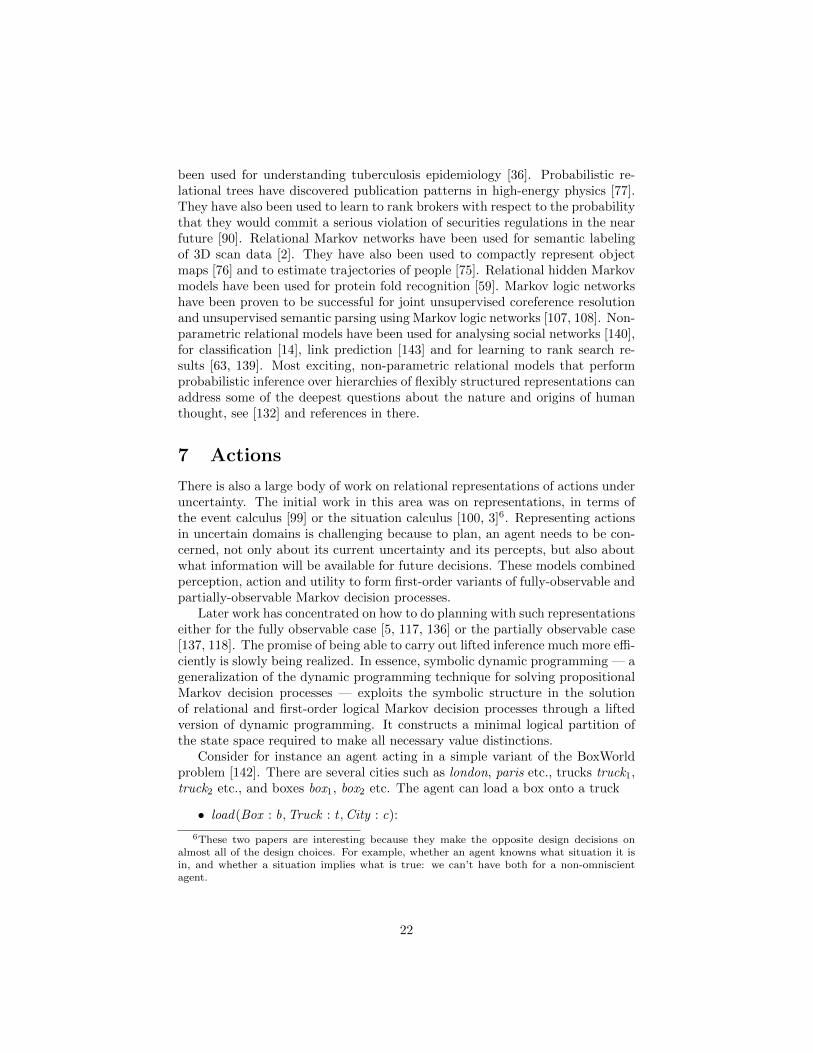
Consider for instance an agent acting in a simple variant of the BoxWorldproblem [142]. There are several cities such as london, paris etc., trucks truck1,truck2 etc., and boxes box1, box2 etc. The agent can load a box onto a truck

• load(Box : b,Truck : t ,City : c):

6These two papers are interesting because they make the opposite design decisions onalmost all of the design choices. For example, whether an agent knowns what situation it isin, and whether a situation implies what is true: we can’t have both for a non-omniscientagent.

22

– Success Probability: if (BoxIn(b, c) ∧ TruckIn(t , c)) then .9 else 0

– Add Effects on Success: {BoxOn(b, t)}– Delete Effects on Success: {BoxIn(b, c)}

or unload it and can drive a truck from one city to another. Only when aparticular box, say box box1, is in a particular city, say paris, the agent receivesa positive reward.

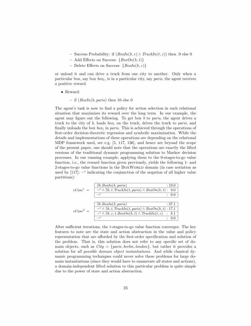
• Reward:

– if (BoxIn(b, paris) then 10 else 0

The agent’s task is now to find a policy for action selection in each relationalsituation that maximizes its reward over the long term. In our example, theagent may figure out the following. To get box b to paris, the agent drives atruck to the city of b, loads box1 on the truck, drives the truck to paris, andfinally unloads the box box1 in paris. This is achieved through the operations offirst-order decision-theoretic regression and symbolic maximization. While thedetails and implementations of these operations are depending on the relationalMDP framework used, see e.g. [5, 117, 136], and hence are beyond the scopeof the present paper, one should note that the operations are exactly the liftedversions of the traditional dynamic programming solution to Markov decisionprocesses. In our running example, applying them to the 0-stages-to-go valuefunction, i.e., the reward function given previously, yields the following 1- and2-stages-to-go value functions in the BoxWorld domain (in case notiation asused by [117]; ¬“ indicating the conjunction of the negation of all higher valuepartitions):

vCase1 =

∃b.BoxIn(b, paris) : 19.0

¬“ ∧ ∃b, t .TruckIn(t , paris) ∧ BoxOn(b, t) : 9.0

¬“ : 0.0

vCase2 =

∃b.BoxIn(b, paris) : 27.1

¬“ ∧ ∃b, t .TruckIn(t , paris) ∧ BoxOn(b, t) : 17.1

¬“ ∧ ∃b, c, t .BoxOn(b, t) ∧ TruckIn(t , c) : 8.1

¬“ : 0.0

After sufficient iterations, the t-stages-to-go value function converges. The keyfeatures to note are the state and action abstraction in the value and policyrepresentation that are afforded by the first-order specification and solution ofthe problem. That is, this solution does not refer to any specific set of do-main objects, such as City = {paris, berlin, london}, but rather it provides asolution for all possible domain object instantiations. And while classical dy-namic programming techniques could never solve these problems for large do-main instantiations (since they would have to enumerate all states and actions),a domain-independent lifted solution to this particular problem is quite simpledue to the power of state and action abstraction.

23

Since the basic symbolic dynamic programming approach, a variety of exactalgorithms have been introduced to solve MDPs with relational and first-orderstructure. First-order value iteration [48, 55] and the relational Bellman al-gorithm [64] are value iteration algorithms for solving relational MDPs. Inaddition, first-order decision diagrams have been introduced to compactly rep-resent case statements and to permit efficient application of symbolic dynamicprogramming operations to solve relational MDPs via value iteration and pol-icy iteration [136]. All of these algorithms have some form of guarantee onconvergence to the (ε-)optimal value function or policy. Furthermore, a class oflinear-value approximation algorithms have been introduced to approximate thevalue function as a linear combination of weighted basis functions. First-orderapproximate linear programming [117] directly approximates the relational valuefunction using a linear program. Other heuristic solutions for instance inducesrule-based policies from sampled experience in small-domain instantiations ofrelational MDPs and generalizes these policies to larger domains [31]. In a sim-ilar vein, Gretton and Thiebaux [43] used the action regression operator inthe situation calculus to provide the first-order hypothesis space for an induc-tive policy learning algorithm. One can also turn the relational MDP into astructured dynamic Bayesian network representation and predict the effects ofaction sequences using approximate inference and beliefs over world states [71].Recently, Lang and Toussaint [70] and Joshi et al. [53] have shown that success-ful planning typically involves only a small subset of relevant objects and haveshown how to make use of this fact to speed up symbolic dynamic programmingsignificantly.

Solvers for relational MDPs have been successfully applied in decision-theoreticplanning domains such as BlocksWorld, BoxWorld, ZenoWorld, Elevators, Drive,PitchCatch and Schedule comparing well to or even outperforming proposi-tional counterparts. Related techniques have been used to solve path planningproblems within robotics and instances of real-time strategy games, Tetris, andDigger.

Finally, there is also work on relational reinforcement learning, see [129, 135]for overviews, where an agent learns what to do before knowing what individ-uals will be encountered, and so before it knows what random variables exist.As an example, consider the idea of having household robots, which just needto be taken out of their shipping boxes, turned on, and then do some cleaningwork. This ”robot-out-of-the-box” has inspired research in robotics as well as inmachine learning and artificial intelligence. Without a compact knowledge rep-resentation that supports abstraction by and unification of logical placeholders,and in turn generalization of previous experiences to the current state and poten-tial future states, however, it seems to be difficult — if not hopeless — to exploreone’s home in reasonable time. There are simply too many objects a householdrobot may deal with such as doors, plates, boxes and water-taps. To deal withthis ”curse of dimensionality”, a number of model-free [29, 27, 28, 26, 110, 60]as well as model-based, see e.g. [92, 71], relational reinforcement learning ap-proaches have been developed. A key insight is that the inherent generalizationof learnt knowledge in the relational representation has profound implications

24

also on the exploration strategy: what in a propositional setting would be con-sidered a novel situation and worth exploration may in the relational settingbe an instance of a well-known context in which exploitation is promising [72].For instance, after having opened one or two water taps in the kitchen, saywt(obj 1), in(obj 1, k1), k(k1) and wt(obj 2), in(obj 2, k2), k(k2), to fill the sinkwith water, the household robot can expect other water-taps to behave similarly.Thus, the priority for exploring water-taps in kitchens wt(X ), in(X ,Y ), k(Y ) ingeneral should be reduced and not just the one for wt(obj 1), in(obj 1, k1), k(k1)and wt(obj 2), in(obj 2, k), in(k2). Moreover, our information gathered aboutwater-taps wt(X ), in(X ,Y ), k(Y ) so far should also transfer to water-taps inlaundries, say wt(obj 3), in(obj 3, l1), l(l1) since we have also learned somethingabout wt(X ), in(X ,Y ). Without extensive feature engineering this would bedifficult — if not impossible — in a propositional setting. We would simplyencounter a new and therefore unexplored situation.

In general, robotics is an emerging application area for StaRAI techniques [4,133]. As robots are starting to perform everyday manipulation tasks, such ascleaning up, setting a table or preparing simple meals, they must become muchmore knowledgeable than they are today. Typically, everyday tasks are specifiedvaguely and the robot must therefore infer what are the appropriate actions totake and which are the appropriate objects involved in order to accomplish thesetasks. These inferences can only be done if the robot has access to general worldknowledge.

8 Identity and Existence Uncertainty

The previously outlined work assumes that an agent knows which individualsexist and can identify them. The problem of knowing whether two descriptionsrefer to the same individual is known as identity uncertainty [91, 102]. Thisarises in citation matching [91] when we need to distinguish whether two ref-erences refer to the same paper and in record linkage [30], where the aim is todetermine if two hospital records refer to the same person (e.g., whether thecurrent patient who is requesting drugs been at the hospital before). To solvethis, we have the hypotheses of which descriptions refer to the same individuals,and which refer to different ones. If there are n descriptions, an assignment ofequality to these descriptions corresponds to a partitioning of the descriptions(each description in a partition corresponds to the same individual, and differ-ent partitions correspond to different individuals). The number of partitions onn elements is the Bell number, which grows faster than any exponential.

The problem of knowing whether some individual exists is known as exis-tence uncertainty [80, 102]. This is challenging because when existence is false,there is no individual to refer to, and when existence is true, there may bemany individuals that fit a description. We may have to know which individ-ual a description is referring to. In general, determining the probability of anobservation requires knowing the protocol for how observations were made. Forexample, if an agent considers a house and declares that there is a green room,

25

the probability of this observation depends on what protocol they were using:did they go looking for a green room, did they report the colour of the firstroom found, did they report the type of the first green thing found, or did theyreport on the colour of the first thing they perceived?

9 Ontologies and Semantic Science

Data that are reliable and people care about, particularly in the sciences, arebeing reported using the vocabulary defined in formal ontologies [32]. The nextstage in this line of research is to represent scientific hypotheses that also referto formal ontologies and are able to make probabilistic predictions that can bejudged against data [104]. This work combines all of the issues of relationalprobabilistic modelling as well as the problems of describing the world at mul-tiple level of abstraction and detail, and handling multiple heterogenous datasets. It also requires new ways to think about ontologies [105], and new waysto think about the relationships between data, hypotheses and decisions.

10 Conclusions

Real agents need to deal with their uncertainty and reason about individuals andrelations. They need to learn how the world works before they have encounteredall the individuals they need to reason about. If we accept these premises,then we need to get serious about relational probabilistic models. There is agrowing community under the umbrella of statistical relational learning that istackling the problems of decision making with models that refer to individualsand relations. While there have been considerable advances in the last twodecades, there are more than enough problems to go around to establish whathas come to be called statistical relational AI.

Acknowledgements Krisitan Kersting was supported by the Fraunhofer AT-TRACT fellowship STREAM and by the European Commission under contractnumber FP7-248258-First-MM. Sriraam Natarajan acknowledges the support ofTranslational Science Institute of Wake Forest University School of Medicine.David Poole is supported by NSERC.

References

[1] Ahmadi, B., Kersting, K., and Hadiji, F. (2010). Lifted belief propagation:Pairwise marginals and beyond. In T.J. P. Myllymaeki T. Roos (Ed.), Pro-ceedings of the 5th European Workshop on Probabilistic Graphical Models(PGM–10). Helsinki, Finland.

[2] Anguelov, D., Taskar, B., Chatalbashev, V., Koller, D., Gupta, D., Heitz,G., and Ng, A. (2005). Discriminative Learning of Markov Random Fields

26

for Segmentation of 3D Scan Data. In C. Schmid, S. Soatto, and C. Tomasi(Eds.), IEEE Computer Society International Conference on ComputerVision and Pattern Recognition (CVPR-05), volume 2, pp. 169–176. SanDiego, CA, USA.

[3] Bacchus, F., Halpern, J.Y., and Levesque, H.J. (1999). Reasoning aboutnoisy sensors and effectors in the situation calculus. Artificial Intelligence,111(1–2): 171–208. URL http://www.lpaig.uwaterloo.ca/~fbacchus/

on-line.html.

[4] Beetz, M., Jain, D., Mosenlechner, L., and Tenorth, M. (2010). Towardsperforming everyday manipulation activities. Robotics and AutonomousSystems, 58.

[5] Boutilier, C., Reiter, R., and Price, B. (2001). Symbolic dynamic pro-gramming for first-order MDPs. In Proc. 17th International Joint Conf.Artificial Intelligence (IJCAI-01).

[6] Breese, J.S. (1992). Construction of belief and decision networks. Com-putational Intelligence, 8(4): 624–647.

[7] Buntine, W.L. (1994). Operations for learning with graphical models.Journal of Artificial Intelligence Research, 2: 159–225.

[8] Carbonetto, P., Kisynski, J., de Freitas, N., and Poole, D. (2005). Non-parametric bayesian logic. In Proc. 21st Conf. on Uncertainty in AI(UAI).

[9] Chavira, M. and Darwiche, A. (2005). Compiling bayesian networks withlocal structure. In Proceedings of the International Joint Conference onArtificial Intelligence (IJCAI), pp. 1306–1312.

[10] Chiang, M. and Poole, D. (2011). Reference classes and relational learning.International Journal of Approximate Reasoning. doi:DOI:10.1016/j.ijar.2011.05.002.

[11] Choi, J., de Salvo Braz, R., and Bui, H. (2011). Efficient methods forlifted inference with aggregate factors. In AAAI 2011.

[12] Choi, J., Guzman-Rivera, A., and Amir, E. (2011). Lifted relationalkalman filtering. In IJCAI, pp. 2092–2099.

[13] Choi, J., Hill, D., and Amir, E. (2010). Lifted inference for relationalcontinuous models. In UAI’10: Proceedings of the Twenty-Sixth Confer-ence on Uncertainty in Artificial Intelligence, pp. 126–134. AUAI Press,Corvallis, Oregon, USA.

[14] Chu, W., Sindhwani, V., Ghahramani, Z., and Keerthi, S. (2006). Rela-tional learning with gaussian processes. In Neural Information ProcessingSystems.

27

[15] Darwiche, A. (2002). A logical approach to factoring belief networks. InProceedings of KR, pp. 409–420.

[16] Darwiche, A. (2001). Recursive conditioning. Artificial Intelligence, 126(1-2): 5–41.

[17] de Finetti, B. (1931). Funzione caratteristica di un fenomeno aleatorio.Atti della R. Accademia Nazionale dei Lincei, Ser. 6. Memorie, Classe diScienze Fisiche, Matematiche e Naturali 4, pp. 251–299.

[18] De Raedt, L. (2008). Logical and Relational Learning. Springer.

[19] De Raedt, L. and Kersting, K. (2003). Probabilistic Logic Learning. ACM-SIGKDD Explorations: Special issue on Multi-Relational Data Mining,5(1): 31–48.

[20] De Raedt, L. and Kersting, K. (2004). Probabilistic Inductive Logic Pro-gramming. In S. Ben-David, J. Case, and A. Maruoka (Eds.), Proceed-ings of the 15th International Conference on Algorithmic Learning Theory(ALT-04), volume 3244 of LNCS, pp. 19–36. Springer, Padova, Italy.

[21] De Raedt, L., Kimmig, A., and Toivonen, H. (2007). ProbLog: A prob-abilistic Prolog and its application in link discovery. In Proceedings ofthe 20th International Joint Conference on Artificial Intelligence (IJCAI-2007), pp. 2462–2467.

[22] De Raedt, L., Frasconi, P., Kersting, K., and Muggleton, S.H. (Eds.)(2008). Probabilistic Inductive Logic Programming. Springer.

[23] de Salvo Braz, R., Natarajan, S., Bui, H., Shavlik, J., and Russell, S.(2009). Anytime lifted belief propagation. In Statistical Relational Learn-ing Workshop.

[24] de Salvo Braz, R., Amir, E., and Roth, D. (2006). Mpe and partialinversion in lifted probabilistic variable elimination. In Proceedings of the21sth National Conference on Artificial Intelligence (AAAI).

[25] de Salvo Braz, R., Amir, E., and Roth, D. (2007). Lifted first-orderprobabilistic inference. In L. Getoor and B. Taskar (Eds.), Introduction toStatistical Relational Learning. M.I.T. Press. URL http://www.cs.uiuc.

edu/~eyal/papers/BrazRothAmir_SRL07.pdf.

[26] Driessens, K. and Dzeroski, S. (2005). Combining model-based andinstance-based learning for first-order regression. In Proc. InternationalConf. on Machine Learning, pp. 193–200.

[27] Driessens, K. and Ramon, J. (2003). Relational instance based regres-sion for relational reinforcement learning. In Proc. International Conf. onMachine Learning, pp. 123–130.

28

[28] Driessens, K., Ramon, J., and Gartner, T. (2006). Graph kernels andGaussian processes for relational reinforcement learning. Machine Learn-ing Journal.

[29] Dzeroski, S., de Raedt, L., and Driessens, K. (2001). Relational reinforce-ment learning. Machine Learning, 43: 7–52.

[30] Fellegi, I. and Sunter, A. (1969). A theory for record linkage. Journal ofthe American Statistical Association, 64(328): 1183–1280.

[31] Fern, A., Yoon, S., and Givan, R. (2003). Approximate policy iterationwith a policy language bias. In NIPS-2003. Vancouver.

[32] Fox, P., McGuinness, D., Middleton, D., Cinquini, L., Darnell, J., Garcia,J., West, P., Benedict, J., and Solomon, S. (2006). Semantically-enabledlarge-scale science data repositories. In 5th International Semantic WebConference (ISWC06), volume 4273 of Lecture Notes in Computer Sci-ence, pp. 792–805. Springer-Verlag. URL http://www.ksl.stanford.

edu/KSL_Abstracts/KSL-06-19.html.

[33] Frey, B.J., Kschischang, F.R., Loeliger, H.A., and Wiberg, N. (1997). Fac-tor graphs and algorithms. In Proceedings of the 35th Allerton Conferenceon Communication, Control, and Computing, pp. 666–680. Champaign-Urbana, IL. URL http://www.psi.toronto.edu/~psi/pubs2/1999%

20and%20before/134.pdf.

[34] Friedman, N., Getoor, L., Koller, D., and Pfeffer, A. (1999). Learningprobabilistic relational models. In Proceedings of the Sixteenth Interna-tional Joint Conference on Artificial Intelligence (IJCAI-99), pp. 1300–1309. Morgan Kaufman, Stockholm, Sweden.

[35] Getoor, L., Friedman, N., Koller, D., and Pfeffer, A. (2001). Learningprobabilistic relational models. In S. Dzeroski and N. Lavrac (Eds.), Re-lational Data Mining, pp. 307–337. Springer-Verlag.

[36] Getoor, L., Rhee, J., Koller, D., and Small, P. (2004). Understandingtuberculosis epidemiology using probabilistic relational models. Journalof Artificial Intelligence in Medicine, 30: 233–256.

[37] Getoor, L., Taskar, B., and Koller, D. (2001). Using probabilistic modelsfor selectivity estimation. In Proceedings of ACM SIGMOD InternationalConference on Management of Data, pp. 461–472. ACM Press.

[38] Getoor, L. and Taskar, B. (Eds.) (2007). Introduction to Statistical Rela-tional Learning. MIT Press, Cambridge, MA.

[39] Gogate, V. and Domingos, P. (2010). Exploiting logical structure in liftedprobabilistic inference. In AAAI 2010 Workshop on Statististical and Re-lational Artificial Intelligence (STAR-AI). URL http://aaai.org/ocs/

index.php/WS/AAAIW10/paper/view/2049.

29

[40] Gogate, V. and Domingos, P. (2011). Probabilistic theorem proving. InProc. 27th Conf. Uncertainty in AI.

[41] Goldman, R.P. and Charniak, E. (1990). Dynamic construction of beliefnetworks. In Proc. 6th Conference on Uncertainty in Artificial Intelli-gence, pp. 90–97.

[42] Goodman, N., Mansinghka, V., Roy, D.M., Bonawitz, K., and Tenenbaum,J. (2008). Church: a language for generative models. In Proc. Uncertaintyin Artificial Intelligence (UAI). URL http://web.mit.edu/droy/www/

papers/church\_GooManRoyBonTenUAI2008.pdf.

[43] Gretton, C. and Thiebaux, S. (2004). Exploiting first-order regression ininductive policy selection. In UAI-04, pp. 217–225. Banff, Canada.

[44] Gutmann, B. and Kersting, K. (2006). Tildecrf: Conditional random fieldsfor logical sequences. In M.S. J. Fuernkranz T. Scheffer (Ed.), Proceedingsof the 17th European Conference on Machine Learning (ECML–2006), pp.174–185. Berlin, Germany.

[45] Hadiji, F., Kersting, K., and Ahmadi, B. (2010). Lifted message passingfor satisfiability. In Working Notes of the AAAI10 Workshop on StatisticalRelational AI (StarAI). AAAI Press.

[46] Heckerman, D. and Breese, J. (1994). A new look at causal independence.In UAI.

[47] Heckerman, D., Meek, C., and Koller, D. (2004). Probabilistic models forrelational data. Technical Report MSR-TR-2004-30, Microsoft Research.

[48] Holldobler, S. and Skvortsova, O. (2004). A logic-based approach to dy-namic programming. In In AAAI-04 Workshop on Learning and Planningin MDPs, pp. 31–36. Menlo Park, CA.

[49] Horsch, M. and Poole, D. (1990). A dynamic approach to probabilisticinference using Bayesian networks. In Proc. Sixth Conference on Uncer-tainty in AI, pp. 155–161. Boston.

[50] Jaeger, M. (2007). Parameter learning for Relational Bayesian networks.In ICML.

[51] Jha, A., Gogate, V., Meliou, A., and Suciu, D. (2010). Lifted inferencefrom the other side: The tractable features. In Twenty-Fourth AnnualConference on Neural Information Processing Systems (NIPS).

[52] Jordan, M.I. (2010). Bayesian nonparametric learning: Expressive priorsfor intelligent systems. In R. Dechter, H. Geffner, and J.Y. Halpern (Eds.),Heuristics, Probability and Causality: A Tribute to Judea Pearl, pp. 167–186. College Publications.

30

[53] Joshi, S., Kersting, K., and Khardon, R. (2010). Self-taught decisiontheoretic planning with first order decision diagrams. In Proceedings ofICAPS-10.

[54] Kallenberg, O. (2005). Probabilistic symmetries and invariance principles.Springer.

[55] Karabaev, E. and Skvortsova, O. (2005). A heuristic search algorithm forsolving first-order MDPs. In UAI-2005, pp. 292–299. Edinburgh, Scotland.

[56] Kemp, C., Tenenbaum, J., Griffiths, T., Yamada, T., and Ueda, N. (2006).Learning systems of concepts with an infinite relational model. In Proc.21st AAAI.

[57] Kersting, K., Ahmadi, B., and Natarajan, S. (2009). Counting beliefpropagation. In J.B. A. Ng (Ed.), Proceedings of the 25th Conference onUncertainty in Artificial Intelligence (UAI–09). Montreal, Canada.

[58] Kersting, K. and De Raedt, L. (2007). Bayesian logic programming: The-ory and tool. In L. Getoor and B. Taskar (Eds.), An Introduction toStatistical Relational Learning. MIT Press.

[59] Kersting, K., De Raedt, L., and Raiko, T. (2006). Logial Hidden MarkovModels. Journal of Artificial Intelligence Research (JAIR), 25: 425–456.

[60] Kersting, K. and Driessens, K. (2008). Non–parametric policy gradients:A unified treatment of propositional and relational domains. In S.R.A. McCallum (Ed.), Proceedings of the 25th International Conference onMachine Learning (ICML 2008). Helsinki, Finland.

[61] Kersting, K. and Driessens, K. (2008). Non-parametric policy gradients: Aunified treatment of propositional and relational domains. In Proceedingsof the 25th International Conference on Machine Learning (ICML).

[62] Kersting, K., Massaoudi, Y.E., Ahmadi, B., and Hadiji, F. (2010). In-formed lifting for message–passing. In D.P. M. Fox (Ed.), Twenty–FourthAAAI Conference on Artificial Intelligence (AAAI–10). AAAI Press, At-lanta, USA.

[63] Kersting, K. and Xu, Z. (2009). Learning preferences with hidden com-mon cause relations. In Proceedings of the European Conference on Ma-chine Learning and Principles and Practice of Knowledge Discovery inDatabases (ECML PKDD 09), LNAI. Springer, Bled, Slovenia.

[64] Kersting, K., van Otterlo, M., and de Raedt, L. (2004). Bellman goesrelational. In ICML-04. ACM Press, Banff, Alberta, Canada. doi:http://doi.acm.org/10.1145/1015330.1015401.

31

[65] Kisynski, J. and Poole, D. (2009). Constraint processing in lifted proba-bilistic inference. In Proc. 25th Conference on Uncertainty in AI, (UAI-2009), pp. 293–302. Montreal, Quebec. URL http://www.cs.ubc.ca/

~poole/papers/KisynskiUAI2009.pdf.

[66] Kisynski, J. and Poole, D. (2009). Lifted aggregation in directed first-orderprobabilistic models. In Proc. Twenty-first International Joint Conferenceon Artificial Intelligence (IJCAI-09), pp. 1922–1929. Pasadena, Califor-nia.

[67] Kok, S. and Domingos, P. (2007). Learning the structure of Markov logicnetworks. In Proc. of the Intern. Conf. on Machine Learning (ICML-05),pp. 441–448.

[68] Kok, S. and Domingos, P. (2009). Learning Markov Logic Network Struc-ture via Hypergraph Lifting. In Proc. of the International Conference onMachine Learning (ICML-09).

[69] Kyburg, H. (1983). The reference class. Philosophy of Science, 50: 374–397.

[70] Lang, T. and Toussaint, M. (2009). Relevance grounding for planning inrelational domains. In Proc. European Conf. on Machine Learning.

[71] Lang, T. and Toussaint, M. (2010). Planning with noisy probabilisticrelational rules. Journal of Artificial Intelligence Research (JAIR), 39:1–49.

[72] Lang, T., Toussaint, M., and Kersting, K. (2010). Exploration in rela-tional worlds. In J. Balcazar, F. Bonchi, A. Gionis, and M. Sebag (Eds.),European Conference on Machine Learning and Principles and Prac-tice of Knowledge Discovery in Databases (ECML PKDD-10). Springer,Barcelona, Spain.

[73] Laskey, K.B. (2008). MEBN: A language for first-order Bayesian knowl-edge bases. Artificial Intelligence, 172(2-3). doi:doi:10.1016/j.artint.2007.09.006. URL http://www.sciencedirect.com/science/article/

B6TYF-4PTMXXP-1/2/ce6bcf1c5a5fecfd805501056e9b62a1.

[74] Lavrac, N. and Dzeroski, S. (1994). Inductive Logic Programming: Tech-niques and Applications. Ellis Horwood, NY.

[75] Liao, L., Fox, D., and Kautz, H. (2005). Location-Based Activity Recog-nition using Relational Markov Networks. In F. Giunchiglia and L.P.Kaelbling (Eds.), Proceedings of the Nineteenth International Joint Con-ference on Artificial Intelligence (IJCAI-05), pp. 773–778. AAAI Press,Edinburgh, Scotland.

32

[76] Limketkai, B., Liao, L., and Fox, D. (2005). Relational Object Maps forMobile Robots. In F. Giunchiglia and L.P. Kaelbling (Eds.), Proceedingsof the Nineteenth International Joint Conference on Artificial Intelligence(IJCAI-05), pp. 1471–1476. AAAI Press, Edinburgh, Scotland.

[77] McGovern, A., Friedland, L., Hay, M., Gallagher, B., Fast, A., Neville,J., and Jensen, D. (2003). Exploiting relational structure to understandpublication patterns in high-energy physics. SIGKDD Explorations, 5(2):165–173.

[78] Mihalkova, L. and Mooney, R. (2007). Bottom-Up Learning of MarkovLogic Network Structure. In Proc. of the Intern. Conf. on Machine Learn-ing (ICML-07).

[79] Mihalkova, L. and Richardson, M. (2009). Speeding up inference in statis-tical relational learning by clustering similar query literals. In In Proceed-ings of the 19th International Conference on Inductive Logic Programming(ILP-09.

[80] Milch, B., Marthi, B., Russell, S., Sontag, D., Ong, D.L., and Kolobov, A.(2005). BLOG: Probabilistic models with unknown objects. In Proc. 19thInternational Joint Conf. Artificial Intelligence (IJCAI-05). Edinburgh.

[81] Milch, B. and Russell, S. (2006). General-purpose mcmc inference overrelational structures. In In Proceedings of the Proceedings of the Twenty-Second Conference Annual Conference on Uncertainty in Artificial Intel-ligence (UAI06, pp. 349–358. AUAI Press.

[82] Milch, B., Zettlemoyer, L.S., Kersting, K., Haimes, M., and Kael-bling, L.P. (2008). Lifted probabilistic inference with counting formu-las. In Proceedings of the Twenty Third Conference on Artificial In-telligence (AAAI). URL http://people.csail.mit.edu/lpk/papers/

mzkhk-aaai08.pdf.

[83] Muggleton, S. (1996). Stochastic logic programs. In L. De Raedt (Ed.),Advances in Inductive Logic Programming, pp. 254–264. IOS Press.

[84] Muggleton, S. and De Raedt, L. (1994). Inductive logic programming:Theory and methods. Journal of Logic Programming, 19,20: 629–679.

[85] Natarajan, S., Khot, T., Kersting, K., Gutmann, B., and Shavlik, J.(2011). Gradient–based boosting for statistical relational learning: Therelational dependency network case. Machine Learning Journal. (OnlineFirst).

[86] Natarajan, S., Tadepalli, P., Dietterich, T.G., and Fern, A. (2009). Learn-ing first-order probabilistic models with combining rules. Special Issue onProbabilistic Relational Learning, AMAI.

33

[87] Natarajan, S., Khot, T., Lowd, D., Tadepalli, P., Kersting, K., Shavlik,J., and Iais, F. (2010). Exploiting causal independence in markov logicnetworks: Combining undirected and directed models. In Proceedings ofECML.

[88] Nath, A. and Domingos, P. (2010). Efficient lifting for online probabilisticinference. In AAAI.

[89] Neumann, M., Kersting, K., and Ahmadi, B. (2011). Markov logic sets:Towards lifted information retrieval using pagerank and label propagation.In D.R. W. Burgard (Ed.), Proceedings of the Twenty–Fifth AAAI Con-ference on Artificial Intelligence (AAAI–11). AAAI Press, San Francisco,CA, USA.

[90] Neville, J., Simsek, O., Jensen, D., Komoroske, J., Palmer, K., and Gold-berg, H. (2005). Using relational knowledge discovery to prevent securitiesfraud. In Proceedings of the 11th ACM SIGKDD International Conferenceon Knowledge Discovery and Data Mining. ACM Press.

[91] Pasula, H., Marthi, B., Milch, B., Russell, S., and Shpitser, I. (2003).Identity uncertainty and citation matching. In NIPS, volume 15.

[92] Pasula, H., Zettlemoyer, L., and Pack Kaelbling, L. (2007). Learningsymbolic models of stochastic domains. Artificial Intelligence Research,29: 309–352.

[93] Pearl, J. (1988). Probabilistic Reasoning in Intelligent Systems: Networksof Plausible Inference. Morgan Kaufmann, San Mateo, CA.

[94] Perlich, C. and Provost, F. (2006). Distribution-based aggregation forrelational learning with identifier attributes. In Machine Learning.

[95] Pfeffer, A. (2007). The design and implementation of IBAL: A general-purpose probabilistic language. In L. Getoor and B. Taskar (Eds.), Sta-tistical Relational Learning. MIT Press.

[96] Poole, D. (1991). Representing diagnostic knowledge for probabilisticHorn abduction. In Proc. 12th International Joint Conf. on ArtificialIntelligence (IJCAI-91), pp. 1129–1135. Sydney.

[97] Poole, D. (1993). Logic programming, abduction and probability: A top-down anytime algorithm for computing prior and posterior probabilities.New Generation Computing, 11(3–4): 377–400.

[98] Poole, D. (1993). Probabilistic Horn abduction and Bayesian networks.Artificial Intelligence, 64(1): 81–129.

[99] Poole, D. (1997). The independent choice logic for modelling multipleagents under uncertainty. Artificial Intelligence, 94: 7–56. URL http:

//cs.ubc.ca/~poole/abstracts/icl.html. Special issue on economicprinciples of multi-agent systems.

34

[100] Poole, D. (1998). Decision theory, the situation calculus and conditionalplans. Electronic Transactions on Artificial Intelligence, 2(1–2). URLhttp://www.etaij.org.

[101] Poole, D. (2003). First-order probabilistic inference. In Proc. EighteenthInternational Joint Conference on Artificial Intelligence (IJCAI-03), pp.985–991. Acapulco, Mexico.

[102] Poole, D. (2007). Logical generative models for probabilistic reasoningabout existence, roles and identity. In 22nd AAAI Conference on AI(AAAI-07). URL http://cs.ubc.ca/~poole/papers/AAAI07-Poole.

pdf.

[103] Poole, D. (2008). The independent choice logic and beyond. In L. DeRaedt, P. Frasconi, K. Kersting, and S. Muggleton (Eds.), Probabilis-tic Inductive Logic Programming: Theory and Application, LNCS 4911.Springer Verlag. URL http://cs.ubc.ca/~poole/papers/ICL-Beyond.

pdf.

[104] Poole, D., Smyth, C., and Sharma, R. (2008). Semantic science: On-tologies, data and probabilistic theories. In P.C. da Costa, C. d’Amato,N. Fanizzi, K.B. Laskey, K. Laskey, T. Lukasiewicz, M. Nickles,and M. Pool (Eds.), Uncertainty Reasoning for the Semantic WebI, LNAI/LNCS. Springer. URL http://cs.ubc.ca/~poole/papers/

SemSciChapter2008.pdf.

[105] Poole, D., Smyth, C., and Sharma, R. (2009). Ontology design forscientific theories that make probabilistic predictions. IEEE IntelligentSystems, 24(1): 27–36. URL http://www2.computer.org/portal/web/

computingnow/2009/0209/x1poo.

[106] Poole, D.L. and Mackworth, A.K. (2010). Artificial Intelligence: foun-dations of computational agents. Cambridge University Press, New York,NY. URL http://artint.info.

[107] Poon, H. and Domingos, P. (2008). Joint unsupervised coreference res-olution with markov logic. In Proceedings of the 2008 Conference onEmpirical Methods in Natural Language Processing (EMNLP). Honolulu,HI, USA.

[108] Poon, H. and Domingos, P. (2009). Unsupervised semantic parsing. InProceedings of the 2009 Conference on Empirical Methods in Natural Lan-guage Processing (EMNLP). Singapore.

[109] Poon, H., Domingos, P., and Sumner, M. (2008). A general method for re-ducing the complexity of relational inference and its application to mcmc.In Proceedings of the 23rd national conference on Artificial intelligence -Volume 2, pp. 1075–1080.

35

[110] Ramon, J., Driessens, K., and Croonenborghs, T. (2007). Transfer learn-ing in reinforcement learning problems through partial policy recycling.In Proc. European Conf. on Machine Learning, pp. 699–707.

[111] Reichenbach, H. (1949). The Theory of Probability. University of Califor-nia Press,.

[112] Richards, B. and Mooney, R. (1992). Learning relations by pathfinding.In M.S. J. Fuernkranz T. Scheffer (Ed.), Proceedings of the 10th NationalConference on Artificial Intelligence (AAAI-92), pp. 174–185. San Jose,CA, USA.

[113] Richardson, M. and Domingos, P. (2006). Markov logic networks. MachineLearning, 62: 107–136.

[114] Riedel, S. (2008). Improving the accuracy and efficiency of map infer-ence for markov logic. In Proceedings of the 24th Annual Conference onUncertainty in AI (UAI ’08), pp. 468–475.

[115] Russell, S. and Norvig, P. (2010). Artificial Intelligence: A Modern Ap-proach. Series in Artificial Intelligence. Prentice Hall, Upper Saddle River,NJ, third edition. URL http://aima.cs.berkeley.edu/.

[116] Sang, T., Beame, P., and Kautz, H. (2005). Solving Bayesian networksby weighted model counting. In Proc. Twentieth National Conference onArtificial Intelligence (AAAI-05), pp. 475–482.

[117] Sanner, S. and Boutilier, C. (2009). Practical solution techniques for firstorder mdps. AIJ, 173: 748–788.

[118] Sanner, S. and Kersting, K. (2010). Symbolic dynamic programming forfirst-order POMDPs. In Proc. AAAI-2010.

[119] Sato, T. and Kameya, Y. (1997). PRISM: A symbolic-statistical modelinglanguage. In Proceedings of the 15th International Joint Conference onArtificial Intelligence (IJCAI-97), pp. 1330–1335.

[120] Sato, T. and Kameya, Y. (2008). New advances in logic-based probabilisticmodeling by PRISM. In L. De Raedt, P. Frasconi, K. Kersting, andS. Muggleton (Eds.), Probabilistic Inductive Logic Programming, volumeLNCS 4911, pp. 118–155. Springer. URL http://www.springerlink.

com/content/1235t75977x62038/.

[121] Segal, E., Battle, A., and Koller, D. (2003). Decomposing gene expres-sion into cellular processes. In Proc. Pacific Symposium on Biocomputing(PSB), pp. 89–100. World Scientific.

[122] Segal, E., Taskar, B., Gasch, A., Friedman, N., and Koller, D. (2001).Rich probabilistic models for gene expression. Bioinformatics, 17(Suppl1): S243–52. Proc. ISMB 2001.

36

[123] Sen, P., Deshpande, A., and Getoor, L. (2008). Exploiting shared corre-lations in probabilistic databases. Proc. VLDB Endow., 1: 809–820.

[124] Sen, P., Deshpande, A., and Getoor, L. (2009). Bisimulation-based ap-proximate lifted inference. In Uncertainty in Artificial Intelligence.

[125] Shafer, G. and Shenoy, P. (1990). Probability propagation. Annals ofMathematics and Artificial Intelligence, 2: 327–352.

[126] Shavlik, J. and Natarajan, S. (2009). Speeding up inference in markovlogic networks by preprocessing to reduce the size of the resultinggrounded network. In Proceedings of the 21st international jont conferenceon Artifical intelligence, pp. 1951–1956.

[127] Silva, R., Chu, W., and Ghahramani, Z. (2007). Hidden common causerelations in relational learning. In Neural Information Processing Systems.

[128] Singla, P. and Domingos, P. (2008). Lifted first-order belief propagation.In Proceedings of the Twenty-Third AAAI Conference on Artificial Intel-ligence, pp. 1094–1099.

[129] Tadepalli, P., Givan, R., and Driessens, K. (2004). Relational reinforce-ment learning: An overview. In Proc. ICML Workshop on RelationalReinforcement Learning.

[130] Talbott, W. (2008). Bayesian epistemology. In E.N. Zalta (Ed.), The Stan-ford Encyclopedia of Philosophy. URL http://plato.stanford.edu/

archives/fall2008/entries/epistemology-bayesian/.

[131] Taskar, B., Abbeel, P., and Koller, D. (2002). Discriminative Probabilis-tic Models for Relational Data. In A. Darwiche and N. Friedman (Eds.),Proceedings of the Eighteenth Conference on Uncertainty in Artificial In-telligence (UAI-02), pp. 485–492. Edmonton, Alberta, Canada.

[132] Tenenbaum, J., Kemp, C., Griffiths, T., and Goodman, N. (2011). Howto grow a mind: Statistics, structure, and abstraction. Science, 331(11March 2011): 1279–1285.

[133] Tenorth, M., Klank, U., Pangercic, D., and Beetz, M. (2011). Web-enabled robots – robots that use the web as an information resource.IEEE Robotics and Automation Magazine, 18.

[134] Van den Broeck, G., Taghipour, N., Meert, W., Davis, J., and De Raedt, L.(2011). Lifted probabilistic inference by first-order knowledge compilation.In Proc. International Joint Conference on AI (IJCAI), pp. 2178–2185.

[135] van Otterlo, M. (2009). The Logic of Adaptive Behavior - KnowledgeRepresentation and Algorithms for Adaptive Sequential Decision Mak-ing under Uncertainty in First-Order and Relational Domains. IOSPress. URL http://people.cs.kuleuven.be/~martijn.vanotterlo/

phdbook_vanOtterlo_v2010a.pdf.

37

[136] Wang, C., Joshi, S., and Khardon, R. (2008). First order decision diagramsfor relational mdps. JAIR, 31: 431–472.

[137] Wang, C. and Khardon, R. (2010). Relational partially observable MDPs.In Proc. AAAI-2010.

[138] Wick, M., McCallum, A., and Miklau, G. (2010). Scalable probabilisticdatabases with factor graphs and mcmc. 3(1): 794–804.

[139] Xu, Z., Kersting, K., and Joachims, T. (2010). Fast active exploration forlink–based preference learning using gaussian processes. In Proceedings ofthe European Conference on Machine Learning and Principles and Prac-tice of Knowledge Discovery in Databases (ECML PKDD–10). Springer,Barcelona, Spain.

[140] Xu, Z., Tresp, V., Rettinger, A., and Kersting, K. (2009). Social net-work mining with nonparametric relational models. In Advances in SocialNetwork Mining and Analysis, LNCS. Springer.

[141] Xu, Z., Tresp, V., Yu, K., and Kriegel, H.P. (2006). Infinite hidden rela-tional models. In Proc. 22nd UAI.

[142] Younes, H., Littman, M., Weissman, D., and Asmuth, J. (2005). The firstprobabilistic track of the international planning competition. JAIR, 24:851–887.

[143] Yu, K. and Chu, W. (2007). Gaussian process models for link analysisand transfer learning. In Neural Information Processing Systems.

[144] Yu, K., Chu, W., Yu, S., Tresp, V., and Xu, Z. (2006). Stochastic re-lational models for discriminative link prediction. In Neural InformationProcessing Systems.

[145] Zettlemoyer, L.S., Pasula, H.M., and Kaelbling, L.P. (2007). Logical par-ticle filtering. In In Proceedings of the Dagstuhl Seminar on Probabilistic,Logical, and Relational Learning.

[146] Zhang, N.L. and Poole, D. (1994). A simple approach to Bayesian networkcomputations. In Proc. 10th Canadian Conference on AI, pp. 171–178.

38