Perception & Psychophysics1985, 37 (4), 286-298

Statistical properties of forced-choicepsychometric functions: Implications

of probit analysis

SUZANNE P. McKEESmith-Kettlewell Institute of Visual Sciences, San Francisco, California

STANLEY A. KLEINCollege of Optometry, University of Houston, Houston, Texas

and

DAVIDA Y. TELLERUniversity of Washington, Seattle, Washington

Probit analysis was applied to the problem of threshold estimation from psychometric func­tions derived from the two-alternative forced-choice (2AFC)method of constant stimuli. Thresholdestimates from 2AFC experiments are surprisingly poor: They are about twice as variable ascorresponding estimates based on the traditional yes-no method of constant stimuli, and theirasymmetrical confidence limits are not readily predicted from conventional standard error for­mulas. All of these faults are exacerbated in small samples. Computer simulations demonstratedthat, for small samples, the probit analysis equations do not give a valid estimate of thresholdvariability. The variability of staircase estimates ofthreshold cannot be less than the variabilityof threshold estimates derived from the method ofconstant stimuli given an optimum placementof trials. Hence our findings also define the minimum variability of all staircase estimators un­der the assumptions of probit analysis.

Forced-choice techniques, in combination with themethod of constant stimuli, are increasingly common inmodem psychophysical studies. In a typical two­alternative forced-choice (2AFC) experiment, a stimulusis presented in one of two possible positions on each ofa series of trials, and the subject judges the position ofthe stimulus on each trial. Several different stimuluslevels, varying along some physical dimension (such asintensity), are presented in random order for a substan­tial number of trials each. In an orderly data set, the sub-

This work was supported by NIH Grants 5 P-3G-EYOO186, ROl­EY03976, ROI-EY04776, and ROI-EY02920 and by the Smith­Kettlewell Eye research Foundation. We thank Polly Feigel, Lou Godio,JacobNaclunias, Walter Makous, and Roger Watt for their helpful criticalcommentary on an earlier version of this manuscript, and DonaldMacLeod for useful conversations on thistopic.GeraldWestheimer wrotethe original probit program for the yes-no case. This program servedas a model for subsequent programs that employed different strategiesto handle the 2AFC case and the simulations. We also want to ac­knowledge considerable assistance from Martha Teghtsoonian and ananonymous reviewer in the editing of the final version. A computer pro­gram for 2AFC probit analysis is available from the first author on writtenrequest. Another program, available from the secondauthor, works withseveral shapes of the psychometric function; it has several options forestimating confidence limits and an option for estimating the upperasymptote.

S. P. McKee's mailing address is: Smith-Kettlewelllnstitute ofYisualSciences, 2232 Webster St., San Francisco, CA 94115.

ject's percent correct will vary from near 50 % (chance)for stimuli too weak to be detected to near 100% for stim­uli that are readily detected. Some empirical or theoreticalcurve is fitted to the data and used to estimate one or moreparameters of the assumed underlying population. Themost commonly estimated value is the threshold, T75 ,

which is the stimulus value needed for the subject to becorrect 75 % of the time. This threshold depends on thelocation along the abscissa of the whole psychometricfunction. The slope of the function may also be of interest.If the cumulative normal curve is used as the theoreticalfunction, the threshold, T75 , corresponds to the mean, p.,and the slope, (3, corresponds to the reciprocal of the stan­dard deviation, (J, of the normal curve (i.e., (J =1/(3).

With normal adult subjects, it is feasible to run 100 ormore trials for each stimulus level. Then error varianceis small, the location and slope of the psychometric func­tion can be judged by eye, and typically no elaboratecurve-fitting or statistical analyses are needed. However,with less docile subjects, such as infants and clinical pa­tients, the number of trials may be restricted, and thestatistical properties of threshold estimates derived fromsmall samples become important. These properties aresurprisingly weak: Threshold estimates derived fromforced-choice data may have unacceptably large standarderrors, and the confidence limits may be asymmetricaland significantly larger than would be naively predicted

Copyright 1985 Psychonomic Society, Inc. 286

FORCED-CHOICE PSYCHOMETRIC FUNCTIONS 287

99.99

50~

o

100

2AFC Function

0_ 3 -2 -1 0 1 2 3

Stimulus (Z Units)

D.

100 B.

Yes·NoFunction

c.

oL.o_3~_2:--_.L..1--:-0---71~2---:3

Stimulus (Z Units)

100 A.

99.98

from the standard error. More than 100 trials are requiredbefore confidence limits become well behaved.

The purpose of this paper is fourfold: (1) to explicatethe reasons for these statistical properties at a simplegraphical level; (2) to describe a common statisticalapproach-probit analysis (Finney, 1971)-that is oftenapplied to yes-no psychophysical data, and to explain itsuse in the 2AFC case; (3) to check the validity of theprobit analysis equations by computer simulation of thesampling distribution of the statistic T7~; (4) to explorethe implications of these results for the use of2AFC tech­niques.

GRAPIDCAL ANALYSIS

For the ideal 2AFC case, where C =0.5 and D = 1.0,the midpoint of the psychometric function occurs at p*= 0.75 and the corresponding stimulus value is desig­nated T7~'

The top row of Figure 1 shows the two idealized psy­chometric functions for yes-no and 2AFC. The right-handordinate of Figure 1B gives the probabilities (P) of theunderlying cumulative normal function that have been re­scaled to fit the left-hand ordinate P*, the percentage cor-

This section provides the reader with an intuitive un­derstanding of the statistical properties of estimates of T7~

derived from 2AFC data, given the assumptions of probitanalysis. Although the results of this graphical analysisare inexact in certain respects (see the appendix), this ap­proach will introduce several concepts that are importantto later sections of this paper. We will begin with an ex­planation of the notation used on the axes of these 2AFCgraphs.

On each trial in the traditional method of constantstimuli as applied to a detection task, the subject is shownone sample from a set of stimuli that vary along somephysical dimension and is asked whether the presentedsample exceeds his criterion ("yes or no?"). Data frommany trials are used to determine the stimulus level neededto produce a particular positive response percentage,usually 50% "yes," corresponding to the midpoint of thepsychometric function. Because the psychometric func­tion generated by this yes-no procedure often resemblesa normal ogive, probit analysis can be used to estimatethe statistical properties of these thresholds.

Probit analysis can also be used to estimate thresholdstatisticsfrom 2AFC data by rescaling the cumulative nor­mal function to extend from a lower asymptote C to anupper asymptote D. In an "ideal" 2AFC task, the per­centage correct varies from 50 % to 100% so that C =0.5 and D = 1.0. C and D are incorporated into probitanalysis by assuming an underlying function in which theprobability (P) goes from 0 to 1.0, and, using Abbott'sformula to obtain a probability (or percentage correct),P*, whose limits are C and D:

§;90

/e- 95

/.

Vl u! e>

Q> 50 8 75

'" Q>

~ '"'"Q> E~ 10 ~ 55

~

Figure I. Grapbical illustration of cumulative normal curves andbinomial variability, for both yes-no (A and C) and 2AFC (B andD) cases, on both linear (A and B) and probability (C and D) or­dinates. In each case, error bars represent ±I standard error forn =100. The abscissa is scaled in Z-units, that is, units ofu, the stan­dard deviation of the cumulative normal curve. In C and D, equaldistances on the ordinate represent equal standard deviations of thecumulative normal curve, so that the cumulative normal is convertedinto a straight line. Zero on the abscissa corresponds to the classi­cal threshold, that is, P=0.5 for the yes-no case and P*=0.75 forthe 2AFC case. The hypothetical stimuli are placed at -I, 0, andI Z-unit; this condition represents the "standard case" for the re­mainder of this paper.

50.01 L....L.._-'-_'------'-_-'-2 -1 0 1

Stimulus (Z Units)

0.02 -2 -1 0 1

Stimulus (Z Units)

recto Usually, the abscissa of a graphed psychometricfunction is scaled in units of the stimulus parameter. Here,the abscissa is scaled in units of the standard deviation,(J, of the cumulative normal function, commonly calledZ-score units. Thus, the stimulus values of -1, 0, and1 correspond to the percentages correct (P*) of 58 %,75%, and 92 % for the 2AFC function and percentages"yes" (P) of 16%, 50%,·and 84% for the yes-no function.

Standard errors for n = 100 trials per sampling pointhave been plotted on both functions at the stimulus valuesof -1, 0, and +1. These standard errors are calculatedfrom the usual formula for a standard error of a propor­tion for random samples of size n drawn from a binomialdistribution: --'/PQ/n for the yes-no case or --./P*Q*/n forthe 2AFC case, where Q=1-P and Q*=1-P*.

For yes-no data, the sampling variability is largest near50% and is symmetrically smaller as one moves towardthe lower and upper asymptotes. But forced-choice dataspan only the range from p* = .5 upward. The samplingvariability is largest at C and smallest at D. Forced-choice

(1)p* = C + (D-C) P.

288 McKEE, KLEIN, AND TELLER

2

D.N=120

B.N= 300

//

//

//, /

/ // /

/ ,/

/ /

// /

/ /

/ ,/ /

//

//

//

/

//

/

50.01 L_-::-Z

--!-L---;;----'---:1,---:Z:-- L_-:!:2-~_1~+-'-~-.;;-­

Stimulus (Z Units)

99.99 A.

N=300

50.01 ..........--'---'-'-'--'--.....

99.99 C.N=120

~ 95oug 75'"E~~ 55

~ 95oug 75'"E'"u~ 55

number of trials per point, k is the number of stimuli,and N = nk is the total number of trials. Figure 2 showsthe effect of varying n (100 vs. 40) and consequently N(300 and 120) for three stimulus values. The graphicalapproach for two cases-fixed (or known) slope and vari­able (or unknown) slope are shown in the left and rightcolumns of Figure 2, respectively. In the fixed-slopecase,the assumed slope equals 1 and only the location parameteris to be estimated; in the variable-slope case, both the lo­cation and the slope are to be estimated.

In the fixed-slope cases, the outer dotted lines delimitthe family of possible lines of slope = 1 that will fall en­tirely within the binomial error bars for the three chosenstimulus values. Similarly; in the corresponding variable­slope cases, the outer dotted lines delimit the family ofall possible straight lines, of whatever slope, that will fallentirely within the same three error bars. The arrowsdropped from the limiting dotted lines to the abscissa pro­vide graphical estimates of the 95 % confidence limits forT75 • It must be emphasized that these graphical estimates

Figure 2. Graphical approximation of confidence limits for theestimate of T,. in the 2AFC case, as influenced by the number oftrials and the assumption of a fixed (or known) slope vs. a variable(or unknown) slope. A-N=300, fixed slope; B-N=300, variableslope; C-N=120, fixed slope; D-N=120, variable slope. Error barsrepresent ±1.96 binomial standard errors for each point. The dot­ted lines represent the outer limits of straight lines that can be fit­ted through the error bars. The horizontal arrow through the datapoint at Z=O spans the distance between the dotted lines, andrepresents a graphical estimate of the confidence limits. The two

• arrows above the abscissa mark the estimated confidence limits.

Linearizing TransformationsThe fitting of a curvilinear function to a set of data is

simplified if the function can be converted into a straightline. In psychophysical practice, data are often plotted on"probability paper," transforming a cumulative normalcurve into a straight line. Equal distances on the ordinateare equal standard deviations of a normal distribution(equal Z-units). Linearized versions of Figures 1A and1B are shown in Figures 1C and 1D. For these curves,the abscissa is also scaled in Z-units, so the slope of thelines is 1.0.

When the cumulative normal ogive is transformed intoa linear function, differences in the value of the slope areexpressed by differential "stretching" along the ordinate.The ends of the error bars are tied to the ordinate andstretch along with it; thus the relative lengths of the errorbars change. For the transformed yes-no case, the errorbars are smallest near 50% and largest in the tails. In the2AFC case, the smallest error bars are at 83% and thelargest errors are found in the lower tail, where the in­fluence of a shallow slope, now translated into a magni­fied distance on the ordinate, is superimposed on the al­ready large binomial variation. The intrinsic variabilityof these functions depends on the magnitude of these er­ror bars. Given the same number of trials, the variabilityof threshold estimates derived from 2AFC data is greaterthan the variability of thresholds based on "yes-no" dataprovided that both types of data are adequately describedby cumulative normal functions with the same value of (J.

data thus have a strong asymmetry, with the data pointsnear 50% being likely to deviate more from their cor­responding population values than do points near 100%.

When a theoretical curve is fitted to the data by probitanalysis, the individual data points are weighted inverselywith their intrinsic binomial variability. Thus, in the 2AFCcase, data points sampled from the lower part of the func­tion will be weighted less heavily, and hence constrainthe fitted curve less, than data points sampled from theupper part of the function.

A second factor influences the degree of constraint ex­erted by a given data point on the curve-fitting process­the slope of the normal ogive at that point. Consider trans­lating a normal ogive laterally until the curve intersectsthe upper or lower end of the error bars. Given error barsof a fixed size, the curve could be moved over a muchlarger range where the slope is shallow than where it issteep. Points far in the tail may have much smallerbinomial variability than those near the midpoint, yet theirinfluence on the curve-fitting process may be negligible.For forced-choice data, points near 50% constrain the fit­ting of the curve very litle indeed, since they suffer bothfrom large error bars and minimal slope.

Confidence LimitsThe 2AFC case is examined further in Figure 2, where

the vertical error bars now represent the 95 % confidencelimits, ±1.96, "';P*Q*/n. Throughout this paper, n is the

FORCED-CHOICE PSYCHOMETRIC FUNCTIONS 289

o

B.x· +0.5

N·300

D.X' -1.0N' 300

,,,

-1

50.01L........._...J.-1.---JC-L-'-_..l­

99.99 C.x·-0.5

N'300

99.99 A.x· +1.0

N'300~.c..i 95

ou 75

fu 55~ ,

I

Figure 3. Graphical illustration of the effect of stimulus placementon the confidence limits of T,. estimated from 2AFC data. All linesand symbols as in Figure 2. Sampling above T,. (A and B) producesonly a small increase in the uncertainty of the estimated T,., andis a better strategy than sampling below T,. (C and D).

PROBIT ANALYSIS APPLIEDTO THE 2AFC EXPERIMENT

Probit analysis is an iterative procedure for fitting a cu­mulative normal curve to a set ofdata, estimating the bestchoice for the parameters of the function according to amaximum likelihood criterion. If there are sufficientdegrees of freedom in the data set and a sufficient num­ber of trials, all parameters associated with the psycho­metric function (p., (J, C, D) can be estimated (see Fin­ney, 1971, chap. 7), but for purposes of the present dis­cussion we assume that C and D are known, so that onlyestimates of 1J. and (J are required.

In the computational scheme described by Finney(1971), the observed probabilities are initially transformedinto Z-units (cf. Figure 1) and a provisional line is fit tothe data either by eye or through some more quantitativeapproach such as a least squares estimate of the y-intercept

will often produce the smallest estimated variance of T75,

a range of stimuli placed somewhat asymmetrically above.T75 will work as well (if the upper asymptote is near100%), whereas displacement of the stimuli much belowT75 leads to a deterioration of the estimates of T75'

Asymmetrical Placement of TrialsSince the binomial errors associated with a 2AFC psy­

chometric function are asymmetrical, sampling above thecenter of the distribution is generally a better choice thansampling below its center. This effect is illustrated inFigure 3 for the variable-slope case.

Figures 3A and B show, for n = 100 trials and a stimu­lus spacing of I, the effect of choosing the stimuli on thehigh side of the distribution. The asymmetrical choice dia­gramed in Figure 3A slightly increases the confidence in­terval for T15 , relative to the symmetrical case shown inthe previous figure (2B). Note, however, that, if the up­per asymptote were less than 1.0, the confidence limitscould increase dramatically. There are some asymmetri­cal choices, such as the one shown in Figure 3B, thatproduce estimates of T75 with a variance nearly equal tosymmetrical sampling. On the other hand, sampling muchbelow the center of the function can have disastrous ef­fects on the variance, as shown in Figure 3D.

In summary, graphical analysis illustrates the follow­ing properties of 2AFC psychometric functions:

(l) The variability of the estimated threshold (T75) inthe 2AFC case is greater than the variability of the esti­mated threshold (T50 ) in the yes-no case.

(2) Estimating both the threshold and the slope in­troduces greater uncertainty in the estimate of T75 thandoes estimating the threshold when the slope is assumedto have some fixed value.

(3) Although the choice of symmetrically placed stimuli

of the confidence limits are inexact (too large) and arepresented only as an intuitive guide. 1

Several inferences can be drawn from Figure 2. First,in each pair of graphs, confidence limits for T75 are largerin the variable-slope case. The need to estimate the slopeparameter results in greater uncertainty in the estimateof T75 than does estimating the location parameter alone.Second, obviously, the confidence limits become largerwith smaller values of N. Third, the confidence limits areasymmetrical. This asymmetry also implies that the con­fidence limits cannot readily be calculated from commonlyused (symmetrical) formulas such as ±1.96 standard er­rors, and that intuitive statistical comparisons based onvalues of the standard error will be misleading.

The optimum placement of trials along the stimulus con­tinuum will vary somewhat for different values of N, andwith the choice of a fixed or variable-slope approach.When the slope is known, it makes sense to place all trialsnear the point that provides maximal information on thelocation of the curve, and this point is the same (83%)for all values ofN. When the slope is unknown, the choiceof stimulus locations involves a careful balancing of twofactors-the magnitudes of the error bars, which are them­selves asymmetrical about T75 , and the vertical separa­tion between the tested points-in order to minimize theconfidence limits for the estimated T75 • The balance willvary with N: the smaller N, the farther displaced fromthe center of the distribution will be the optimal stimulusvalues.

290 McKEE, KLEIN, AND TELLER

Standard ErrorsAn attractive feature of probit analysis is that it can pro­

vide quantitative estimates of the standard error of esti­mation of T75. In probit analysis, the simplest analytic for­mula for the standard error of the mean (Finney, 1971,p. 33) is

and the slope. Since observations with smaller error bars(Figure 1) reduce uncertainty about the location and slopeof the best-fitting function more than do observations withlarge error bars, differential weights are then assigned tothe points on the provisional line. The weighting coeffi­cients, w, depend directly on the slope of the cumulativenormal function at the tested stimuli and inversely onP*Q*. Each point is also weighted in direct proportionto n, the number of trials for that stimulus. The probitcalculation can now employ the statistical structure ofweighted linear regression to estimate a best-fitting func­tion. The regression procedure is performed repeatedlyso that successive estimates of the parameters convergeon the maximum likelihood estimates of the y-intercept,a, and the slope, {3. These parameters are simply relatedto the mean and standard deviation of the normal func­tion: p.=-af{3 and (J= lI{3.

1

b..JEnw(2)

these calculations, we assumed a cumulative normal curvewith p.=0 and (J= 1, so the slope of the function is 1. Thus,for the standard case, the sampled stimuli fall at -1,0,and +1 Z-units, corresponding to percents correct (P*)of 58%, 75 %, and 92 % for 2AFC and to percents yesof 16%,50%, and 84%, for yes-no. Because the stimu­lus values are given in Z-units, the calculated standarderror will also be in Z-units. For example, if the stan­dard error is 1 Z-unit, then the uncertainty about the lo­cation of T75 extends over most of the region covered bythe psychometric function, that is, from the stimulus valuecorresponding to 58% to the value corresponding to 92%.

In Figure 4, we have plotted the calculated standard er­rors for the yes-no and 2AFC techniques as a functionof N, along with a line that falls as ..IN. The line is dis­placed rightward by a factor of about 4 for the 2AFC case;about 4 times as many trials must be used in 2AFC asin yes-no to achieve the same value of the standard er­ror. For any particular sample size, assuming that thevalue of (J remains constant across changes in psy­chophysical technique, the standard error for 2AFC isroughly twice the size of the standard error found withyes-no techniques. In a sense, this relationship is expectedbecause the slope of the 2AFC technique is half the valueof the slope for the yes-no technique, as is apparent whenFigures lA and IB are compared.

where b is the sample estimate of the slope {3 of the trans­formed function, and Enw is the sum of the products ofthe probit weights w and the number of trials n for eachtested stimulus.

This formula is a variation of the common statisticalformula sf..IN used to estimate the standard error of themean, because b is the reciprocal of the sample standarddeviation, s, and Enw, the weighted sum of the numberof trials at each point, is used in place of N. In otherwords, in probit analysis, as in other realms of paramet­ric statistics, the standard error of estimation of the meandepends directly on the sample standard deviation, s, andinversely on the square root of the number of trials. Useof this simple "fixed slope" formula for the standard er­ror will result in a serious underestimation of the truevalue of the standard error if the total number of trialsis small, or if the sampled observations are not centerednear T75 • A better estimate of the standard error is givenby the following "variable-slope" formula (Finney, 1971,p.34):

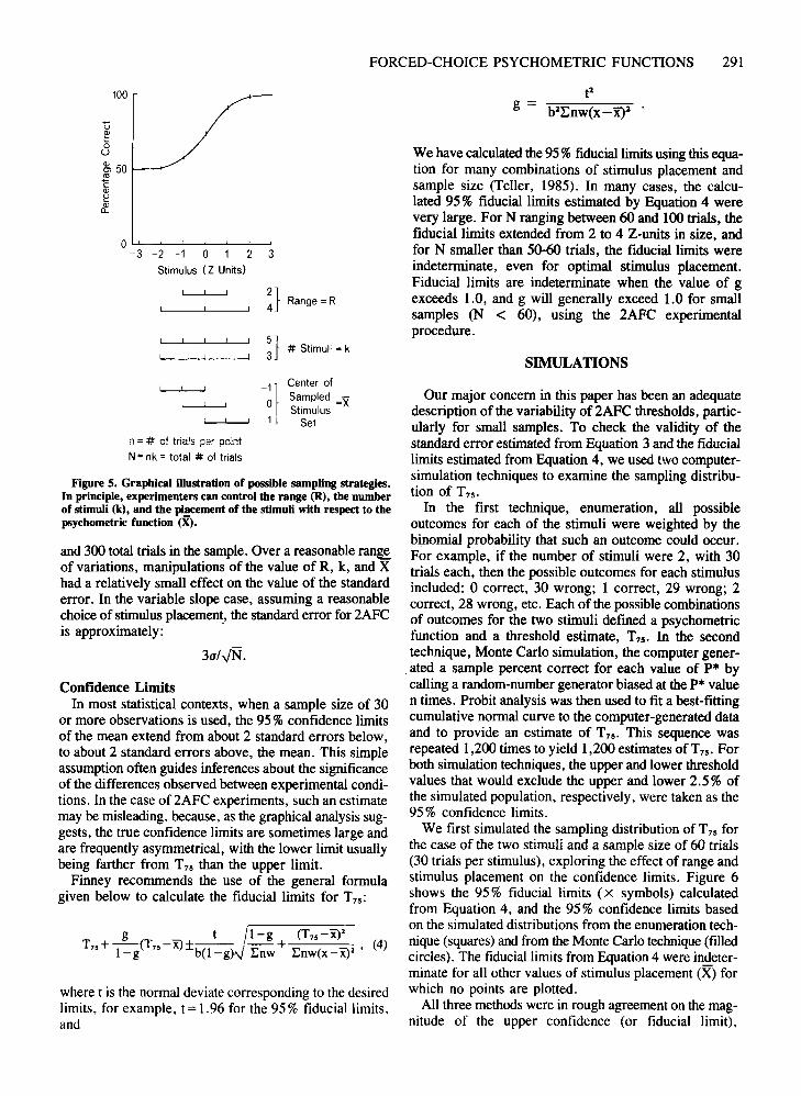
Sampling StrategiesClearly, the experimenter wishes to sample the stimu­

lus domain in a way that provides unbiased, minimum var­iance estimates of T75. In principle, the experimenter canchoose the range, the number of sampled stimuli, and theregion of the stimulus domain sampled with respect to thepsychometric function. To compare sampling strategies,we compute the standard error of T75 for different ranges(R), different numbers of stimuli (k), and different regionsof the stimulus domain, as specified by the center (X) ofthe sampled stimulus set. These choices are diagramedin Figure 5. Calculations were performed with 60, 120,

SE = lib1 (T75-X)1

Enw + Enw(x-X)l' (3)

10.0

gUJ...,~ 0.1cos

U5

0= Y-N.= 2AFC

where x is the weighted mean of the sampled stimulusarray, and lIEnw(x - X)1 is the variance of the slope.

Predictably, the most important parameter controllingthe magnitude of the standard error is sample size. UsingEquation 3, we calculated the standard error as a functionof the total number of trials (N) for one condition, whichwe call the standard case (see Figures lA and IB). For

0.01'----'-----'----'-----'1 10 100 1,000 10,000

Total Number of Trials

Figure 4. The standard error as a function of the total numberof trials for the standard case of Figure 1. The continuous lines showpredicted change if standard errors decreased as a function of.IN. The standard error of T75 estimated from 2AFC data is abouttwice the size of the standard error of T.o estimated from yes-notechnique, assuming the same value of a for both techniques.

FORCED-CHOICE PSYCHOMETRIC FUNCTIONS 291

3

100

Ow...-----'~--'-___J_._'____'_____J

-3 -2 -1 0 1 2

Stimulus (Z Units)

4

2} Range =R

~} # Stimuli = k

Center of

Sampled =XStimulus

Set

n = # of trials per point

N= nk = total # of trials

Figure S. Graphical illustration of possible sampling strategies.In principle, experimenters can control the range (R), the numberof stimuli (k), and the placement of the stimuli with respect to thepsychometric function 00.

and 300 total trials in the sample. Over a reasonable ran~of variations, manipulations of the value of R, k, and Xhad a relatively small effect on the value of the standarderror. In the variable slope case, assuming a reasonablechoice of stimulus placement, the standard error for 2AFCis approximately: .

3u/-.jN.

Confidence LimitsIn most statistical contexts, when a sample size of 30

or more observations is used, the 95 % confidence limitsof the mean extend from about 2 standard errors below,to about 2 standard errors above, the mean. This simpleassumption often guides inferences about the significanceof the differences observed between experimental condi­tions. In the case of2AFC experiments, such an estimatemay be misleading, because, as the graphical analysis sug­gests, the true confidence limits are sometimes large andare frequently asymmetrical, with the lower limit usuallybeing farther from T7S than the upper limit.

Finney recommends the use of the general formulagiven below to calculate the fiducial limits for T7S:

T g T t JI-g (T75 - X)'75+-1- ( 75-X)±b-(1) -r-+ E ( W' (4)-g -g ....nw nw x-x

where t is the normal deviate corresponding to the desiredlimits, for example. t =1.96 for the 95 % fiducial limits.and

We have calculated the 95 % fiducial limits using this equa­tion for many combinations of stimulus placement andsample size (Teller, 1985). In many cases, the calcu­lated 95 % fiducial limits estimated by Equation 4 werevery large. For N ranging between 60 and 100 trials, thefiducial limits extended from 2 to 4 Z-units in size, andfor N smaller than 50-60 trials, the fiducial limits wereindeterminate, even for optimal stimulus placement.Fiducial limits are indeterminate when the value of gexceeds 1.0, and g will generally exceed 1.0 for smallsamples (N < 60), using the 2AFC experimentalprocedure.

SIMULATIONS

Our major concern in this paper has been an adequatedescription of the variability of 2AFC thresholds, partic­ularly for small samples. To check the validity of thestandard error estimated from Equation 3 and the fiduciallimits estimated from Equation 4, we used 1'....0 computer­simulation techniques to examine the sampling distribu­tion of T7s •

In the first technique, enumeration, all possibleoutcomes for each of the stimuli were weighted by thebinomial probability that such an outcome could occur.For example, if the number of stimuli were 2, with 30trials each, then the possible outcomes for each stimulusincluded: 0 correct, 30 wrong; 1 correct, 29 wrong; 2correct, 28 wrong, etc. Each of the possible combinationsof outcomes for the two stimuli defined a psychometricfunction and a threshold estimate, T75 • In the secondtechnique, Monte Carlo simulation, the computer gener­

.ated a sample percent correct for each value of p* bycalling a random-number generator biased at the p* valuen times. Probit analysis was then used to fit a best-fittingcumulative normal curve to the computer-generated dataand to provide an estimate of T75 • This sequence wasrepeated 1,200 times to yield 1,200 estimates ofT75 • Forboth simulation techniques, the upper and lower thresholdvalues that would exclude the upper and lower 2.5 % ofthe simulated population, respectively, were taken as the95% confidence limits.

We first simulated the sampling distribution of T75 forthe case of the two stimuli and a sample size of 60 trials(30 trials per stimulus). exploring the effect of range andstimulus placement on the confidence limits. Figure 6shows the 95 % fiducial limits (X symbols) calculatedfrom Equation 4, and the 95 % confidence limits basedon the simulated distributions from the enumeration tech­nique (squares) and from the Monte Carlo technique (filledcircles). The fiducial limits from Equation 4 were indeter­minate for all other values of stimulus placement (X) forwhich no points are plotted.

All three methods were in rough agreement on the mag­nitude of the upper confidence (or fiducial limit),

292 McKEE, KLEIN, AND TELLER

x-----x CALCULATED VALUES. 0--0 ENUMERATED VALUES. -- SIMULATED VALUES

N =60. K-2 N =60. K =2

RANGE'2.0RANGE =1.5

. . .., ..~--

RANGE '2.5 RANGE·3.0

,/x.i->:-¥.

f-1.0 -0.5 0.5 1.0 1.5

Figure 6. Confidence limits of the estimated value ofT,. for N =60, k=2 for different ranges(R=1.5, 2.0, 2.5, 3.0) as a function ofstimulus placement as indicated by the center of sam­pled set 00. The dotted line (xl sbows the confidence limits calculated from equation (4).The dasbed line (0) shows the simulated confidence limits found with the enumeration tech­nique. The continuous line (e) shows the simulated confidence limits found with the MonteCarlo technique.

which hovered at a value of about twice the calculatedstandard error for values of X near the center of thepsychometric function or above it. The lower fiducial limitfrom Equation 4 was typically much larger than thesimulated values. We concluded that this equation failedto give an accurate estimate of the confidence limits ofsmall 2AFC samples.

Equation 4 is based on an approximation that could beinappropriate for small samples and a high value of C,for example, 0.5 for the 2AFC case. Finney (1971) statesthat well-behaved data almost always give a value of gsubstantially smaller than 1.0 and usually less than 0.4.For the 2AFC case, we found that the value of g gener­ally exceeds 0.4 when the total number of trials is lessthan 130, and often is greater than 1.0 even for optimallyplaced stimuli when N is less than 60 trials.

The patterns of results from the two simulation tech­niques were quite similar, although generally the MonteCarlo technique produced somewhat smaller values.' Theconfidence limits estimated by enumeration are a moreaccurate representation of the true characteristics of theunderlying sampling distribution of T75 • However, theenumeration approach sometimes led to counterintuitiveconclusions. Consider the confidence limits from theenumerations shown in the right-hand comer of Figure 6

for R=3 and X= 1.5. The true percents correct for thetwo stimuli falling at 0 and 3 corresponded to 75% and99.9%, respectively, and, therefore, the most commonvalue associated with the stimulus at 3 Z-units was 30correct, 0 wrong. Mathematically, 100% correct isinfinitelyfar from the center of a cumulative normal distri­bution. Thus, the psychometric function for this enumer­ated condition was often infinitely steep. The estimatedvalue of T75 was the stimulus value corresponding to theother percent correct, which in this case was 0, since thebest-fitting function frequently consisted of a vertical linethrough O. The residual variation in T75 depended onlyon those cases in which the percent correct at 3 Z-unitswas less than 100%, so the confidence limits estimatedby enumeration for this point were very small.

This peculiar case revealed a danger in small­sample-variable-slope estimation, particularly for k=2.As the number of trials per stimulus is decreased, thechance of infinitely steep functions is increased. If, forexample, only 10 trials had been used for each of twostimulus levels corresponding to true percents correct of58% and 92%, then more than 80% of the functionswouldbe infinitely steep, because one of the stimuli would haveproduced a percent equal to or below 50% or equal to100%. Infinitely steep psychometric functions contain lit-

FORCED-CHOICE PSYCHOMETRIC FUNCTIONS 293

N -150STANDARD ERROR -0.22STIMULI = H. o. 1)CONFIDENCE LIMITS:

-0.47. +0.42

-4.0 -3.5 -3.0 -2.5 -2.0 -1.5 -1.0

CUMULATIVE PERCENT-

N-60STANDARD ERROR -0.35STIMULI- (-1. O. 1)

CONFIDENCE LIMITS:-1.3. +0.7

-4.0 -3.5 -3.0 -2.5 -2.0 -1.5

CUMULATIVE PERCENT- 2.5

MEAN

'.

1.0

1.0

1.5

1.5

2.0

2.0

N-45STANDARD ERROR - 0.41STIMULI - H. O.1)CONFIDENCE LIMITS:

-3.2. +0.8

-4.0 -3.5 -3.0 -2.5 -2.0 -1.5

2.5 CUMULATIVE PERCENT-

MEAN

1.5 2.0

N-30STANDARD ERROR - 0.50STIMULI - H. O. 1)

CONFIDENCE LIMITS:-3.7.1.4

-4.0 -3.5 -3.0 -2.5 -2.0 -1.5

2.5 CUMULATIVE PERCENT_

MEAN

2.0

Figure 7. The simulated sampling distributions of tbe estimated value of T7. for tbe stan­dard case for four different values of N, tbe total number of trials. Distributions based on1,200 simulated values using tbe Monte Carlo technique. The curve drawn through tbe pointsis a normal distribution witb a standard deviation equal to tbe calculated standard error(Equation 3) for the indicated sample size. The vertical lines show ±l and ±2 standard er­rors. The arrows under the abscissas indicate tbe stimulus values that correspond to cu­mulative percentages of simulated values of 2.5%, 16%, 84%, and 97.5%. The arrow la­beled "mean" is the average of all simulated values falling between ±4Z-units.

tIe information about the location of the mean and shouldbe avoided, either by increasing the number of stimuliand the number of trials or by constraining the slope'supper limit. 3

Because of the substantial agreement between the twosimulation techniques, we used only the Monte Carlotechnique (l ,200 simulations) to explore other questionsrelated to sampling strategies. The influence of the total

number of trials N on the shape of the sampling distribu­tions of T7S is shown in Figure 7 for the standard case.We have plotted the number of simulated values fallingwithin intervals 0.25 Z-units wide for a range extendingover ±2 Z-units. The arrows on the abscissas, labeled"Mean," point to the average of all the simulated valuesof T7S falling between ±4 Z-units for each distribution.The curve superimposed on each set of points is a normal

294 McKEE, KLEIN, AND TELLER

distribution with a standard deviation equal to the standarderror calculated from Equation 3 for this sample size. Thevertical lines cutting through the normal curves demar­cate ±1 and ±2 calculated standard errors. On the abscissaof each graph, arrows have been drawn to show the valuethat includes ±34% of the simulated distribution and±47.5% of the stimulated distribution, that is, at thecumulative percentages of the simulated distributioncorresponding to 2.5%, 16%, 84%, and 97.5%. If thesampling distribution is normally distributed, the arrowsshould fall near the vertical lines denoting ± 1 and ±2standard errors, and clearly they do not for the three lowerdistributions.

Three trends were apparent in the simulated samplingdistributions as N decreased. First, the width of the dis­tributions increased; second, the confidence limits wereno longer equal to twice the calculated standard error; andthird, the distributions were asymmetrical. In short, thesimulations confirmed our qualitative observations basedon the graphical approach. For N = 150 trials, thesimulated sampling distribution is close to a normal distri­bution, but for N=6O, 45, or 30, the distributions arebadly skewed, a skew sufficient to produce a small biasin the mean of the distribution toward the negative side.The observed asymmetry is a property of 2AFC distri­butions, since the simulated sampling distribution forthresholds estimated from the yes-no psychometricfunctions is perfectly symmetrical and is well fit by a

normal curve even when the total number of trials (N)is as small as 60.

Sampling strategies (Figure 5) can markedly influenceboth the magnitude of the confidence limits and theirasymmetry. In an extended series of simulations of N = 60,we manipulated the range (R), number of stimuli (k), andthe center of the sampled set (X). The results of thesesimulations are plotted in Figure 8. Generally, thesimulated confidence interval is larger than ±2 standarderrors, which, for 60 trials, should be equal to about ±a.8Z-units.

Range had a relatively small effect on the size of thelimits, but sampling with a small range placed a strongconstraint on the placement of the stimuli. For the smallestrange, small shifts in the position of the stimuli led to arapid increase in the limits, whereas for the largest range,the limits remained roughly constant for large shifts inthe center of the sampled stimulus set. As expected,displacements of the center of the sampled stimulus settoward the high end of the psychometric function wererelatively innocuous, whereas equal displacements towardthe low end of the function typically produced large varia­bility in the estimated threshold.

For all ranges, the smallest and most symmetrical limitswere found with k=2. When a small number of stimuliwas used to estimate psychometric functions, the numberof trials per stimulus was obviously larger for k=2, withthe effect that the intrinsic binomial variability of each

RANGE-2.0

••• .0 •••

s-ecRANGE-1.5

RANGE-U

)/

I

N-eo

-1.0 -0.5 0 0.5 1.0 1.5 -1.5 -1.0 -0.5 0 0.5 1.0 1.5CENTER OF SAMPLED STIMULUS SET (~)

e

~ :321

o~----------

~ -12 -2:;, -3

i I::~--,-----,-~--......ul.""'":::I 5

Pl01-----------

-1

-2II: -3

~ -4.... -5~--...Io--'---'--........-..L...-.......

Figure 8. The confidencelimits of the estimated value of T7'based on Monte Carlo simu­lations of N=60 for four values of range. As a function of stimulus placement 00, thecontinuous line (e) shows the limits for k=2; the dotted line (0) shows the limits for k=3;the dashed line (6) shows the limits for k=5.

FORCED-CHOICE PSYCHOMETRIC FUNCTIONS 295

sampled point was smaller. Thus, curves with very shal­low slopes were less common the smaller the number oftested stimuli. This benefit diminished as the range in­creased. Because the chance of observing a psychomet­ric function with an infinitely steep slope is substantialfor k=2, a better strategy for small samples is the choiceof three to five stimuli and a large range.

Our results from the simulations led to the followingconclusions about the statistical properties of 2AFC psy­chometric functions:

(1) For N < 60, the sampling distribution of the esti­mate of T75 is not normally distributed, but is skewed,usually in a negative direction. The skew is sufficient tointroduce a small bias in the estimator.

(2) For small N, the probit analysis equations do notadequately characterize the standard error and the confi­dence limits associated with the estimate of T75.

(3) For small N, sampling with two stimulus values(k=2) will produce the smallest confidence interval, butthe probability of encountering samples with percentscorrect less than or equal to 50%, or equal to 100%, isquite high. Since such samples cannot provide an adequateestimate of the slope of the psychometric function, sam­pling with three stimuli (k= 3) is a better strategy.

(4) For small N, sampling with widely spaced stimuliwill generally yield more stable confidence intervals overa broader range of stimulus placements, whereas samplingwith closely spaced stimuli will make the choice of stimu­lus placement critical.

DISCUSSION

The statistical properties of thresholds estimated from2AFC methods are surprisingly poor, a fact that is notwidely recognized. We have argued here that thresholdestimates derived from 2AFC techniques are about twiceas variable as corresponding estimates derived from yes­no methods and that confidence limits are large, asym­metrical, and not readily predictable from conventionalstandard error formulas. All of these faults are exacer­bated for small samples. The confidence limits for T75in 2AFC experiments do not become well behaved untilNs of 100 or more trials are used. Two questions remain:Are these conclusions inescapable? Are there alternativeapproaches by which these characteristics can be mini­mized or avoided?

The Stimulus DomainThe importance of these conclusions obviously depends

on the steepness of the psychometric functions expected,the degree of accuracy sought in the estimate of T75, andthe number of trials available. Throughout the presentpaper, the stimuli, standard errors, and confidence limitsare scaled in units of a, the standard deviation of the un­derlying cumulative normal curve. When psychometricfunctions are steep in the stimulus domain (a is small),

the standard error and the confidence limits are cor­respondingly small in that domain, and a given error ofestimation of Tv, in Z-units becomes less serious. On theother hand, as psychometric functions become flatter orthe degree of accuracy needed becomes greater in thestimulus domain, the statistical properties ofestimates ofT75 become more important.

Experimental DesignSome practical guidelines for the design of 2AFC ex­

periments follow from the influence of various factors onthe magnitude of standard errors and confidence limits.In the typical case, the only factors the experimenter cancontrol exactly are Nand k; the range (R) and stimulusplacement (X) are defined with respect to T75 and a. Theoptimal placement of trials depends on how much infor­mation the experimenter brings to the experiment. Ifvalues of T75 and a are already rather well known,Figure 8 can be used as a guide to the optimal placementof trials for small samples. If the value of T75 is known,but the value of a is less well known, the range coveredby the stimuli should be broadened, because, as Finney(1971, p. 143) says, "a misjudgement causing the actualresponses to be a little closer to (T75) than was intendedmay be catastrophic, whereas responses a little wider apartthan intended will usually have less serious conse­quences."

IfT75is not known with any degree ofaccuracy-if onemust necessarily run the risk ofa large difference betweenthe center of the sample set (X) and T75-a larger num­ber of more widely spaced stimulus values must, ofcourse, be used, with the expectation that some of thestimuli will be essentially wasted. What is perhaps lessobvious is that when T75 is not known with any degreeof accuracu it is better to err in the direction of positivevalues of X, that is, in the direction of placing one's

. stimuli too high rather than too low. The asymmetries ofbinomial variability lead to the fact that standard errorsand confidence intervals change less for positive than fornegative shifts of equal magnitude.

Data Selection RulesAt the end of the experiment, the experimenter has a

new source of knowledge, the data themselves. In prac­tice, experimenters do not apply statistical analysis blindlyto data; rather, they apply ad hoc or explicit criteria toeach data set, discarding those data sets that do not yieldreasonable estimates of the threshold. For this reason, thesimulated distributions of threshold estimates will not bematched in practice.

Discarding of data obviously has disadvantages. In it­self, it is not a solution to the problem of small N, be­cause when data sets are discarded, trials are wasted. Inaddition, unless the criteria for discarding data are for­mally defined prior to the experiment, discarding dataopens the door to experimenter bias. It might be interest­ing to simulate the use of the 2AFC method of constant

296 McK~E, KLEIN, AND TELLER

stimuli, generating artificial data sets and using a seriesof formal criteria for the discarding of data. Some rulesfor discarding data (e.g., discard data sets that do not con­form to a previously designated goodness-of-fit criterion)may create a sampling distribution for small samples withmore favorable dispersion properties-smaller standarderrors and confidence intervals." It should be possible toseek out and specify data selection rules that provide anoptimum benefit/loss ratio, maximizing the goodness ofthe statisticaldistribution of estimates, while keeping smallthe number of worthwhile data sets discarded.

Staircase MethodsThe most popular strategy for estimating a threshold

from a small sample is the use of staircases or other adap­tive procedures (Cornsweet, 1962; Hall, 1981; Watson& Pelli, 1983; Watt & Andrews, 1981). Staircases haveone obvious advantage over the method of constantstimuli-the efficient use of trials when little is knownabout the location of the desired threshold. A well­designed staircase rule will usually place most of the trialsin the steeper part of the psychometric function rather thanfar in the tails. It is sometimes assumed, erroneously inour view, that because staircase estimates of thresholdsare efficient, they are always much less variable than anyestimate based on the method of constant stimuli. But stair­cases have no magical power. The accuracy of estimatesderived from staircases is constrained by the same fac­tors as is the accuracy of estimation from data collectedby the method of constant stimuli-the number of trials,binomial variability, and the shape of the psychometricfunction. The variability of estimates derived from stair­case data can never be less than the variability of esti­mates derived from the method of constant stimuli selectedfor the optimal deployment of trials.

This assertion can be supported on numerical as wellas logical grounds. Rose, Teller, and Rendleman (1970)used a computer simulation technique to generate stan­dard errors of estimation for 2AFC staircase. These simu­lated standard errors can be compared with the standarderrors estimated from Equation 3 in the present paper for

the 2AFC method of constant stimuli." A selected com­bination of parameters from the two studies, matched asclosely as possible in terms of stimulus spacing (step size)and number of trials, is listed in Table 1. As expected,the standard errors of the staircase estimates sometimesapproach, but are never smaller than, the standard errorsof estimates from the method of constant stimuli with op­timal placement of trials when comparable step sizes andnumber of trials are used.

Alternative Procedures When N Is SmallWe have only a few suggestions for alternative ap­

proaches in situations allowing fewer than 100 trials. Ifone can assume a cumulative normal function with theupper asymptote D= 100%, the threshold criterion canbe shifted from 75 % to 83%, where the intrinsic erroris minimal. This shift is not advisable if the upper aymp­tote is below 98 %, as is common with inattentive sub­jects. If the tested population is well characterized andthe slope of the psychometric function known, it mightbe reasonable to use a fixed slope approach, where theavailable data are used to estimate only the locationparameter. Any difference between the assumed fixedslope and the true slope of the tested individual may in­troduce a bias in the estimate, but this cost may be toler­able given the necessary imprecision inherent in the useof small N.

Instead of attempting to estimate a threshold with aninadequate number of trials, one could test each subjecton only a single stimulus value. On the basis of prior nor­mative data, that value could be chosen to be high on thepsychometric function, perhaps at 83 %, in the regionwhere the intrinsic error is smallest for average normalsubjects. The distribution of performance levels for nor­mal subjects could be established. An individual subject'sor patient's performance below the normal range at thatstimulus value would then indicate a deficit with respectto the normal population. An approach similar to this onehas been used recently to screen infants for possible visualdeficits (Dobson, Teller, Lee, & Wade, 1978; Fulton,Manning, & Dobson, 1978).

Table 1Comparison of Standard Errors for 2AFC Staircases and 2AFC Method of Constant Stimuli

2AFC Staircases (Rose et al., 1971) 2AFC Method of Constant Stimuli

Step Size Number of Number of SE Step Size Number of Optimal SE*(Z-units) Intervals Trials (Z-units) (Z-units) k Range Trials (Z-units)

0.26 10 50 0.30 0.25 5 1 50 0.33200 0.20 200 0.16

0.51 5 50 0.40 0.50 5 2 50 0.37200 0.26 200 0.18

0.64 4 50 0.40 0.66 5 2.5 50 0.40200 0.20 200 0.20

1.28 2 50 0.66 1.25 3 2.5 51 0.42200 0.20 201 0.21

2.56 50 0.97 2.50 2 2.5 50 0.49200 0.56 200 0.24

*For given values of range and k, the SE given is the minimum value found over all values of X; that is.the optimum placement of trials is chosen.

FORCED-CHOICE PSYCHOMETRIC FUNCTIONS 297

In summary, the statistical properties of forced-choicemethods are poorer than might be wished. Although a fewalternatives remain to be explored, we believe that thisvariability is largely unavoidable and will have to be takeninto account in the design and interpretation of forced­choice experiments.

We conclude with the reminder that statistical samplingfluctuations provide only one source of the variability inreal experiments, and that the minimization of othersources of bias and variability must be combined withstatistical theory in the design of experiments to be per­formed on real subjects.

REFERENCES

CORNSWEET, T. N. (1962). The staircase method in psychophysics.American Journal of Psychology, 75, 485-491.

DOBSON, Y., TELLER, D. Y., LEE, C. P., & WADE, B. (1978). A be­havioral method for efficient screening of visual acuity in young in­fants. I. Preliminary laboratory development. Investigative Ophthal­mologyand Visual Science, 17, 1142-1150.

FINNEY, D. J. (1971). Probitanalysis. Cambridge: The University Press.FULTON, A., MANNING, K., & DOBSON, V. (1978). A behavioral method

for efficient screening of visual acuity in young infants. 11. Clinicalapplication. Investigative Ophthalmology and Visual Science, 17,1151-1157.

HALL, J. L. (1981). Hybrid adaptive procedure for estimation of psycho­metric functions. Journal of the Acoustical Society ofAmerica, 69,1763-1769.

ROSE, R., TELLER, D. Y., & RENDLEMAN, P. (1970). Statistical proper­ties of staircase estimates. Perception & Psychophysics, 8,199-204.

TELLER, D. Y. (1985). Psychophysics of infant vision: Definitions andlimitations. In G. Gottlieb & N. Krasnegor (Eds.), Measurement ofaudition and vision in the first year ofpostnatal life: A methodologi­cal overview. Norwood, NJ: Ablex.

WATSON, A. B., & PELLI,D. G. (1983). QUEST: A Bayesian adaptivepsychometric method. Perception & Psychophysics, 33, 113-120.

WATT, R. J., & ANDREWS, D. P. (1981). APE: Adaptive probit estima­tion of psychometric functions. Current Psychological Reviews, 1,205-214.

NOTES

1. Qualitatively speaking, the intervals are too large because the ver­tical bars represent individual confidence intervals for n = 100 trials perpoint, whereas the confidence limits for T" should reflect the joint prob­ability of obtaining all three data points, with a total N of 300 (see ap­pendix for quantitative formulation).

2. The differences between the two techniques reflected differencesin programming strategies, choices usually made to prevent program

"crashes" during the long simulation runs. For example, in the enumer­ation approach, negative or zero slopes were replaced by a very smallSlope (0.001) in order to assign the estimated value of T" to the cor­rect tail of the distribution. In the Monte Carlo approach, a specialproblem arose in assigning a value to percents correct either equal to100% or equal to or below 50 %. Mathematically, these values lay in­finitely far from the center of a cumulative normal distribution. In theMonte Carlo simulations, these percentages were initially assigned avalue of 4 Z-units. Embedded in the probit analysis program was aniterative routine which oscillated between functions corresponding tothese initial values and functions based on much larger values. For theseextreme percentages, the program failed to converge, and after six iter­ations, the value of T" from the last estimated psychometric functionwas stored, and the program continued on to the next data set.

3. The probability of an infinite slope for k = 2 is high even for N = 60and stimuli placed near the center of the psychometric function. Thereis about a 30% chance that one of the two stimuli will fall at .5 or be­low or at 1.0 if the true percents correct = .58 and .92 (-lor +1 unit).If k = 3 and the tested stimuli cover the same range (-1, 0, 1), thereis only about a 6 % chance of an infinite slope.

4. Alternatively, constraints can be placed on the slopes. For exam­pIe, consider the case of 20 trials at each of the locations Z = -O. 5 andZ = + 1.5. Table 2 shows that confidence limits estimated by enumera­ation are -1.9 and +1.5. These enumerations were calculated with theslopes constrained to lie between 0 and 00. If the upper slope constraintwere strengthened to have the slope between 0 and 3, the confidencelimits would become -1.9 and 1.2. If the slope were further constrainedto be greater than .33, the confidence limits would become -1.35 and1.2. Thus, a fairly loose constraint on the slope is able to produce asignificant reduction in the size of the confidence interval.

5. Since the parameter of range is unspecified in staircase techniques,we have converted the units of both Rose et aI. and the present paperto "step size, " that is, to the spacing of adjacent stimuli along thestimulusdimension. Conversion of units was carried out as follows. Rose et aI.used a ramp psychometric function, and scaled the stimulus axis in termsof the interval I. - I, between the lower and upper ends of the ramp.Ancillary simulations showed that ramp and cumulative normal func­tions yielded quantitatively similar standard errors of estimation. In­spection of Rose et aI.'s assumptions and the normal table shows thatthe interval 10 - I. corresponds to 2.56 Z-units in our terms, Rose et al,used the number of intervals between 10- I. as their parameter of stimulusspacing. That is, if adjacent stimuli were so spaced as to fall at 10 andI.. the number of intervals between I., I. is 1 and the step size is 2.56Z-units; if stimuli fall at 10, I" and halfway between, the number ofintervals is 2 and the step size is 1.28 Z-units. In the parameter spaceof the present paper, the step size is the range divided by the quantity,k-I; thus, if k=3 and R=2, the step size is 1 Z-unit.

APPENDIX

Graphical AnalysisIn Figures 2 and 3, a qualitative graphical analysis was used

to determine confidence limits on the threshold estimate. These

Stimuli

Table 295CJ1> Confidence Limits

K = 2, R = 2.0, X = 0(-1,1)

K = 2, R = 2.0, X = .5(-0.5, 1.5)

N

1.96 SE (Equation 3)Finney (Equation 4)EnumerationMonte CarloGraphical Analysis

(Maximum Likelihood)Graphical Analysis

(chi-square)

40

-1.01, 1.01indeterminate-1.6, 1.0-1.4,0.8-1.4, 1.0

-1.2, 1.4

60

-.83, .83-3.0,0.7-1.0, 1.0-1.0,0.6-1.0, 1.0

-0.9, 1.0

40

-.93, .93indeterminate-1.9, 1.5-1.8, 1.3-1.7,1.5

-1.6, 1.5

60

-.76, .76-1.6, 0.7-1.1,1.5-0.9, 1.1-1.0, 1.5

-1.0, 1.5

298 McKEE, KLEIN, AND TELLER

where

where D and C are the upper and lower asymptotes. Thus, Equa­tion Al can be written as

(D-C)~P == -=- exp( -Z'I2)!::.Z, (A2)

.,J27r

The weighting function 11a'zi is precisely the weighting func­tion w, defined and tabulated by Finney (1971).

The optimal values for threshold and slope would be thosevalues that minimize chi-square. When the threshold or slopedeviate from the optimal values, the chi-square will increase.The threshold value that increases chi-square to 1.0 (allowingthe slope to adjust to a new optimal value) corresponds to the68% confidence limit. An increase in chi-square to 4 correspondsto the 95% confidence limit. One of us (Klein) has a probit anal­ysis program available that includes an option for printing outa two-dimensional array of values of chi-square for all valuesof threshold and slope.

A similar discussion applies when using the likelihood func­tion rather than chi-square, except that a change in the logarithmof the likelihood function is half the corresponding change inchi-square.

In Table 2, we compare the 95% confidence limits for severalstimulus locations and for several methods of analysis. The max­imum likelihood graphical analysis corresponds quite closely(within 15%) to the exact confidence limits given by the enumer­ations. The chi-square analysis is almost as good, with signifi­cant errors only for the case of 20 trials and stimuli at + 1 and-1 Z-units. Finney's formula, given by Equation 4, has a largedisagreement with the enumerations, as does +1.96 SE. Thus,maximum likelihood graphical analysis is a highly satisfactorymethod for estimating confidence limits.

(A3)

(AI)x' == E(POi - PEi)'lapi',i

where api' == PEi(l- PEi)/ni and PE is the underlying expectedprobability and POi is the observed probability. If the difference~p == PO-PE is small, then the numerator can be convertedto z-scores.

limits were obtained by shifting the position of a straight-linefit in such a way that the threshold was brought to an extremevalue, subject to the constraint that the line not lie outside theerror bars of any data point. A modification of the constraintbased on the chi-square function enables graphical analysis tohave quantitative validity.

The chi-square function can be written as

21rPEi(l- PEi)exp(Zi')

ni(D-C)'(Manuscript received October 29, 1982;

revision accepted for publication February 25, 1985.)