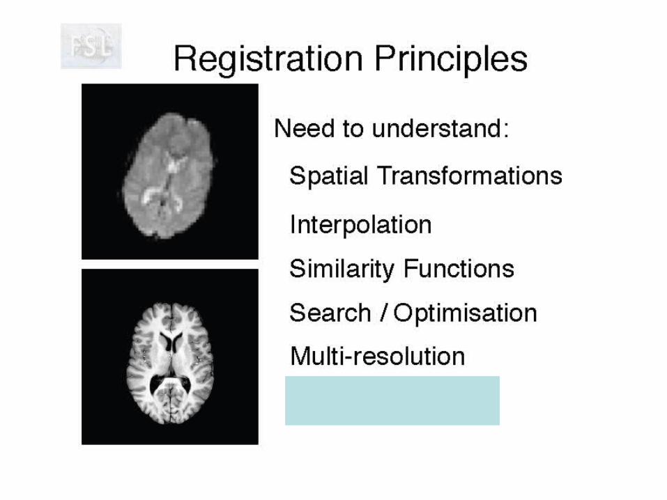
Statistical Parametric MappingStatistical Parametric Mapping

Lecture 11 - Chapter 13Head motion and correction

Textbook: Functional MRI an introduction to methods, Peter Jezzard, Paul Matthews, and Stephen Smith

Many thanks to those that share their MRI slides online

http://www.fmrib.ox.ac.uk/fsl/

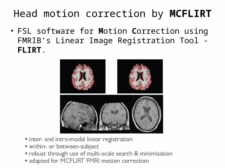
Head motion correction by MCFLIRT• FSL software for Motion Correction using FMRIB’s

Linear Image Registration Tool - FLIRT.

1

43

2

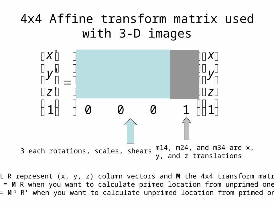
4x4 Affine transform matrix used with 3-D images

⎥⎥⎥⎥

⎦

⎤

⎢⎢⎢⎢

⎣

⎡

⎥⎥⎥⎥

⎦

⎤

⎢⎢⎢⎢

⎣

⎡=

⎥⎥⎥⎥

⎦

⎤

⎢⎢⎢⎢

⎣

⎡

11000343332312423222114131211

1'''

zyx

mmmmmmmmmmmm

zyx

m14, m24, and m34 are x, y, and z translations

3 each rotations, scales, shears

Let R represent (x, y, z) column vectors and M the 4x4 transform matrixR’ = M R when you want to calculate primed location from unprimed oneR = M-1 R’ when you want to calculate unprimed location from primed one

€

x 'y 'z'1

⎡

⎣

⎢ ⎢ ⎢ ⎢

⎤

⎦

⎥ ⎥ ⎥ ⎥=

1 0 0 Tx0 1 0 Ty0 0 1 Tz0 0 0 1

⎡

⎣

⎢ ⎢ ⎢ ⎢

⎤

⎦

⎥ ⎥ ⎥ ⎥

xyz1

⎡

⎣

⎢ ⎢ ⎢ ⎢

⎤

⎦

⎥ ⎥ ⎥ ⎥

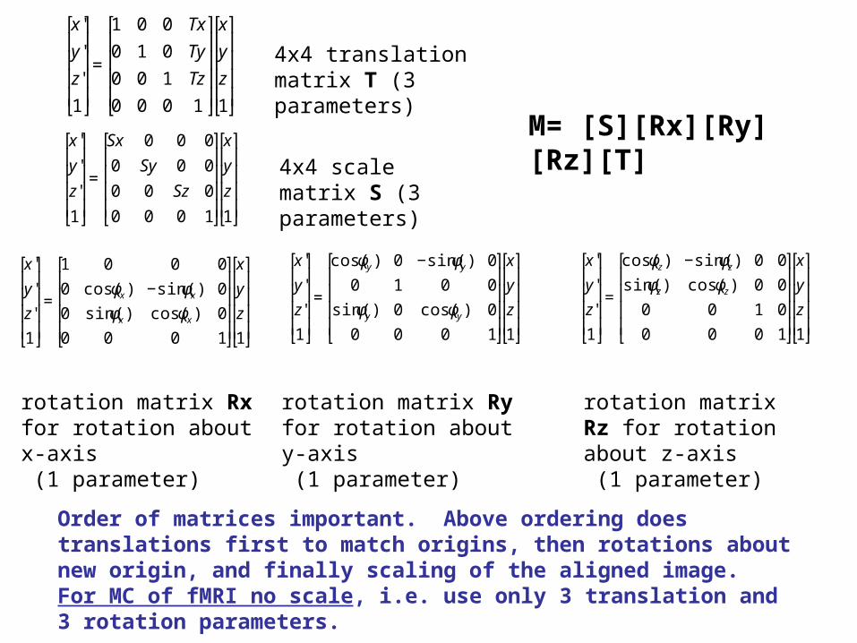
4x4 translation matrix T (3 parameters)

€

x 'y 'z'1

⎡

⎣

⎢ ⎢ ⎢ ⎢

⎤

⎦

⎥ ⎥ ⎥ ⎥=

1 0 0 00 cos(φx ) −sin(φx ) 00 sin(φx ) cos(φx ) 00 0 0 1

⎡

⎣

⎢ ⎢ ⎢ ⎢

⎤

⎦

⎥ ⎥ ⎥ ⎥

xyz1

⎡

⎣

⎢ ⎢ ⎢ ⎢

⎤

⎦

⎥ ⎥ ⎥ ⎥

4x4 scale matrix S (3 parameters)

€

x 'y 'z'1

⎡

⎣

⎢ ⎢ ⎢ ⎢

⎤

⎦

⎥ ⎥ ⎥ ⎥=

Sx 0 0 00 Sy 0 00 0 Sz 00 0 0 1

⎡

⎣

⎢ ⎢ ⎢ ⎢

⎤

⎦

⎥ ⎥ ⎥ ⎥

xyz1

⎡

⎣

⎢ ⎢ ⎢ ⎢

⎤

⎦

⎥ ⎥ ⎥ ⎥

€

x 'y 'z'1

⎡

⎣

⎢ ⎢ ⎢ ⎢

⎤

⎦

⎥ ⎥ ⎥ ⎥=

cos(φy ) 0 −sin(φy ) 00 1 0 0

sin(φy ) 0 cos(φy ) 00 0 0 1

⎡

⎣

⎢ ⎢ ⎢ ⎢

⎤

⎦

⎥ ⎥ ⎥ ⎥

xyz1

⎡

⎣

⎢ ⎢ ⎢ ⎢

⎤

⎦

⎥ ⎥ ⎥ ⎥

€

x 'y 'z'1

⎡

⎣

⎢ ⎢ ⎢ ⎢

⎤

⎦

⎥ ⎥ ⎥ ⎥=

cos(φz) −sin(φz) 0 0sin(φz) cos(φz) 0 0

0 0 1 00 0 0 1

⎡

⎣

⎢ ⎢ ⎢ ⎢

⎤

⎦

⎥ ⎥ ⎥ ⎥

xyz1

⎡

⎣

⎢ ⎢ ⎢ ⎢

⎤

⎦

⎥ ⎥ ⎥ ⎥

rotation matrix Rx for rotation about x-axis (1 parameter)

rotation matrix Ry for rotation about y-axis (1 parameter)

rotation matrix Rz for rotation about z-axis (1 parameter)

M= [S][Rx][Ry][Rz][T]

Order of matrices important. Above ordering does translations first to match origins, then rotations about new origin, and finally scaling of the aligned image. For MC of fMRI no scale, i.e. use only 3 translation and 3 rotation parameters.

1

43

2

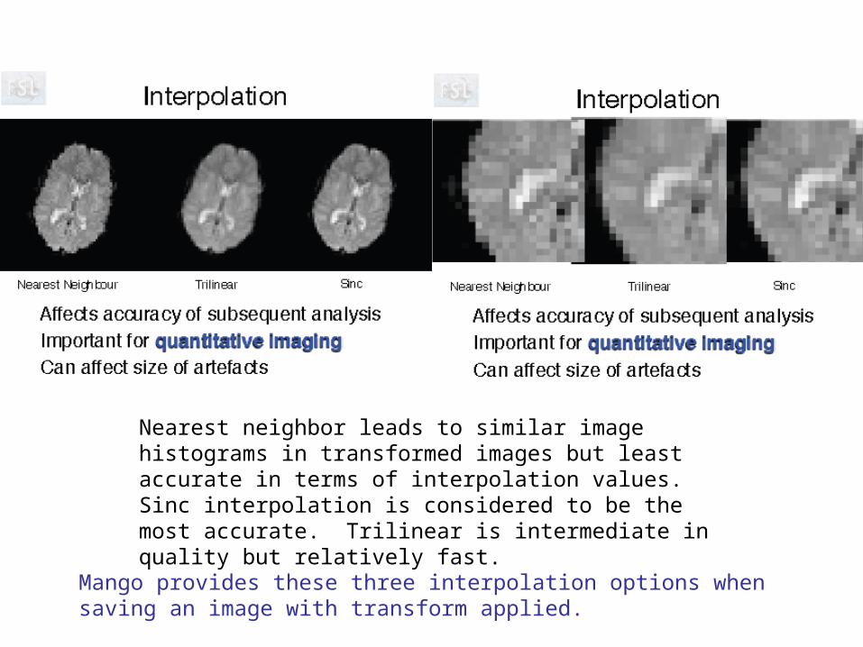
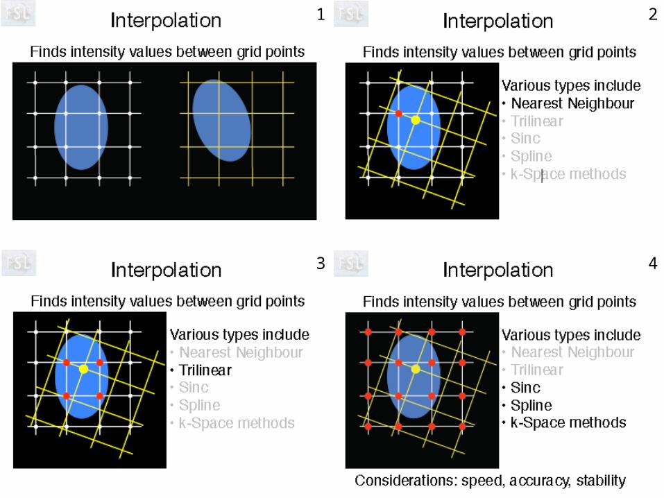
Mango provides these three interpolation options when saving an image with transform applied.

Nearest neighbor leads to similar image histograms in transformed images but least accurate in terms of interpolation values. Sinc interpolation is considered to be the most accurate. Trilinear is intermediate in quality but relatively fast.

1

43

2

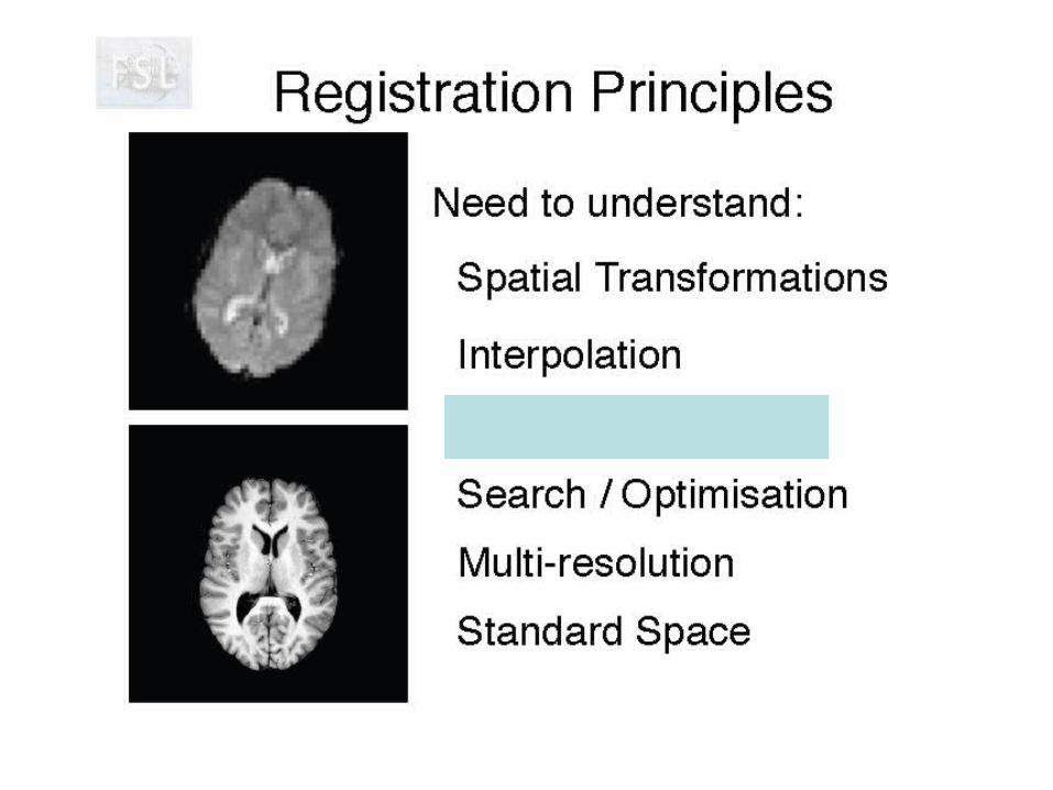
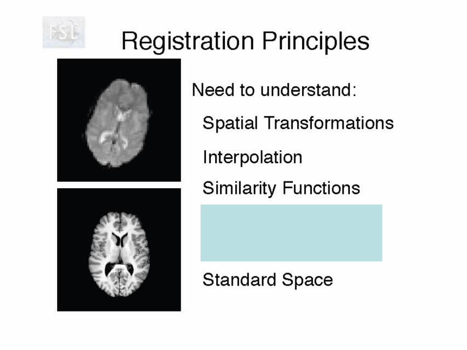
Motion Correction

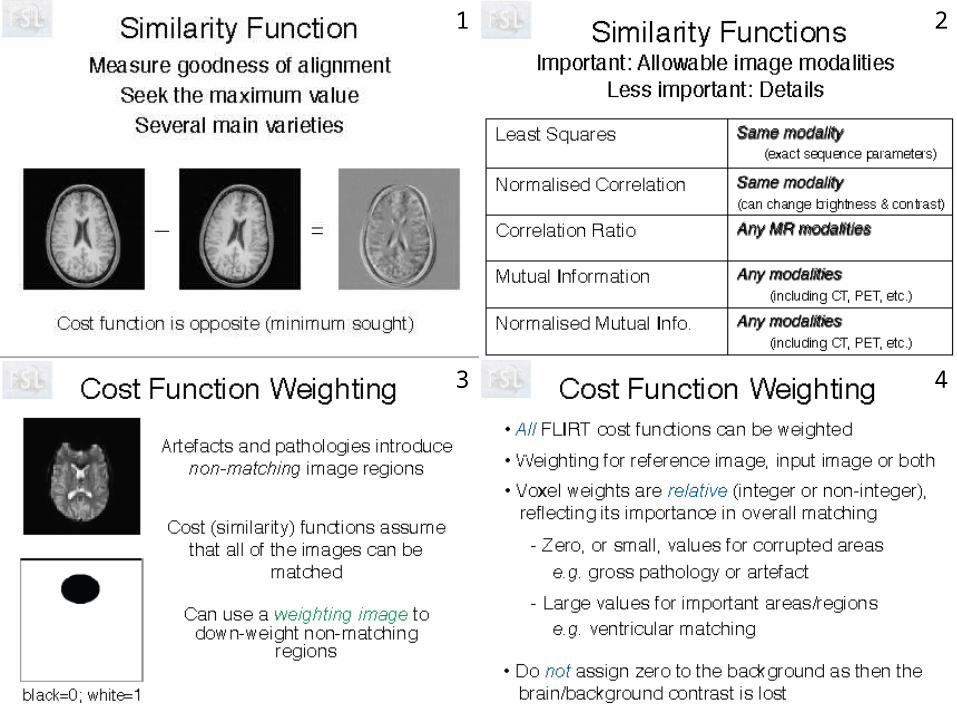
Same Modality

1

43

2

1

3

2

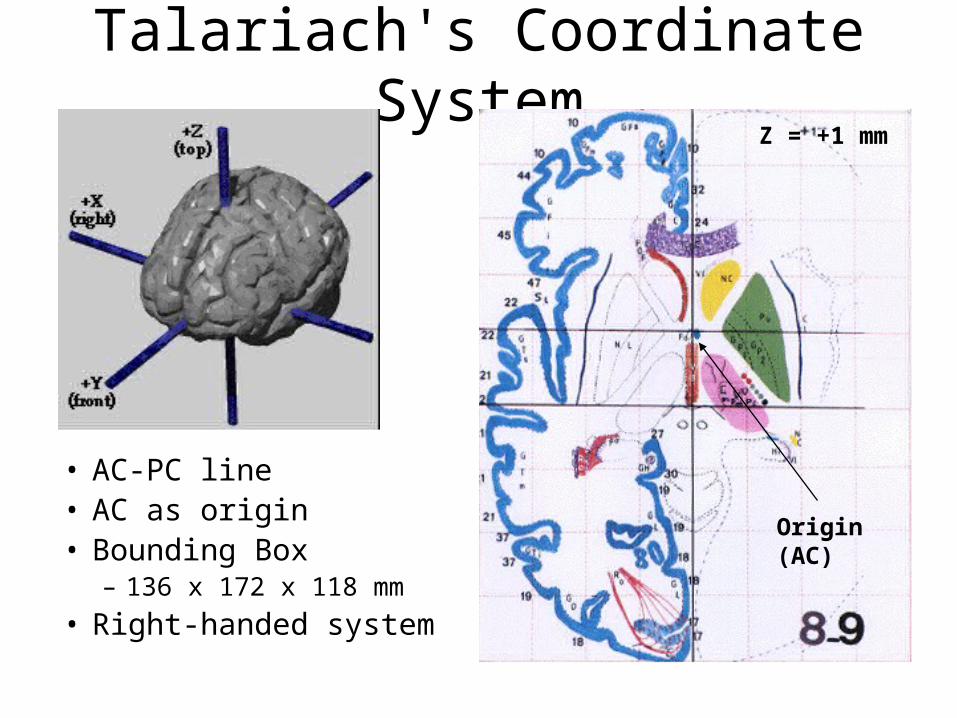
Talariach's Coordinate System

• AC-PC line• AC as origin• Bounding Box

– 136 x 172 x 118 mm• Right-handed system

Z = +1 mm

Origin(AC)

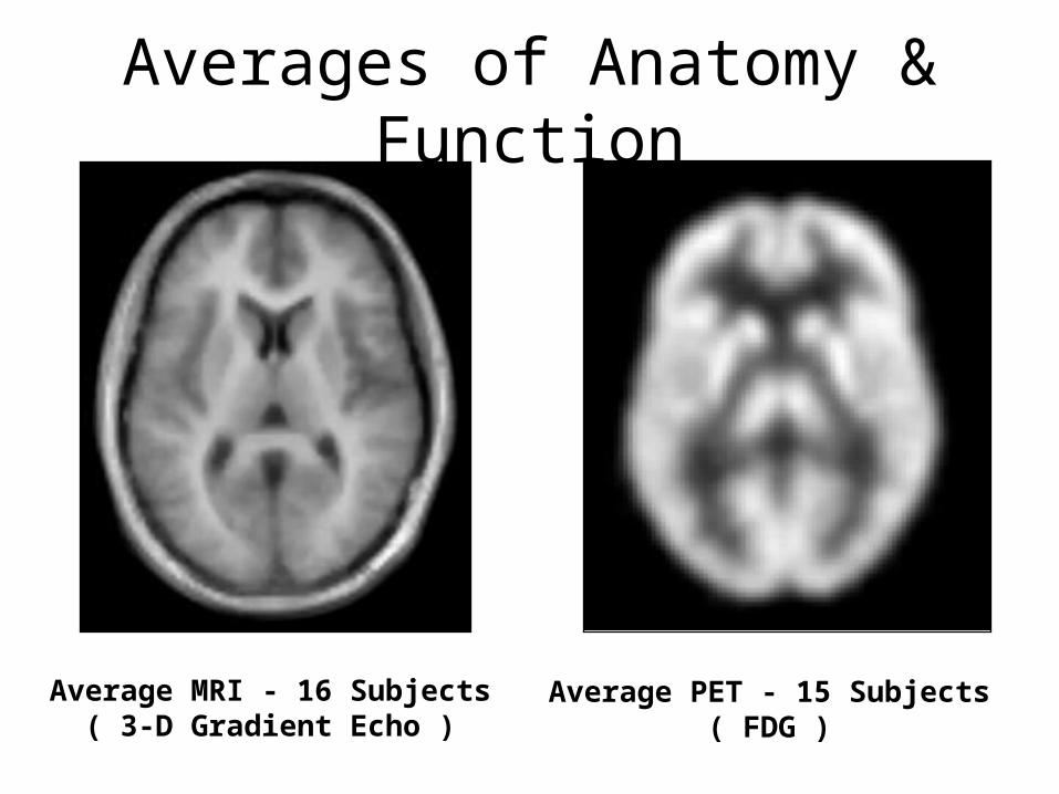
Averages of Anatomy & Function

Average MRI - 16 Subjects( 3-D Gradient Echo )

Average PET - 15 Subjects( FDG )

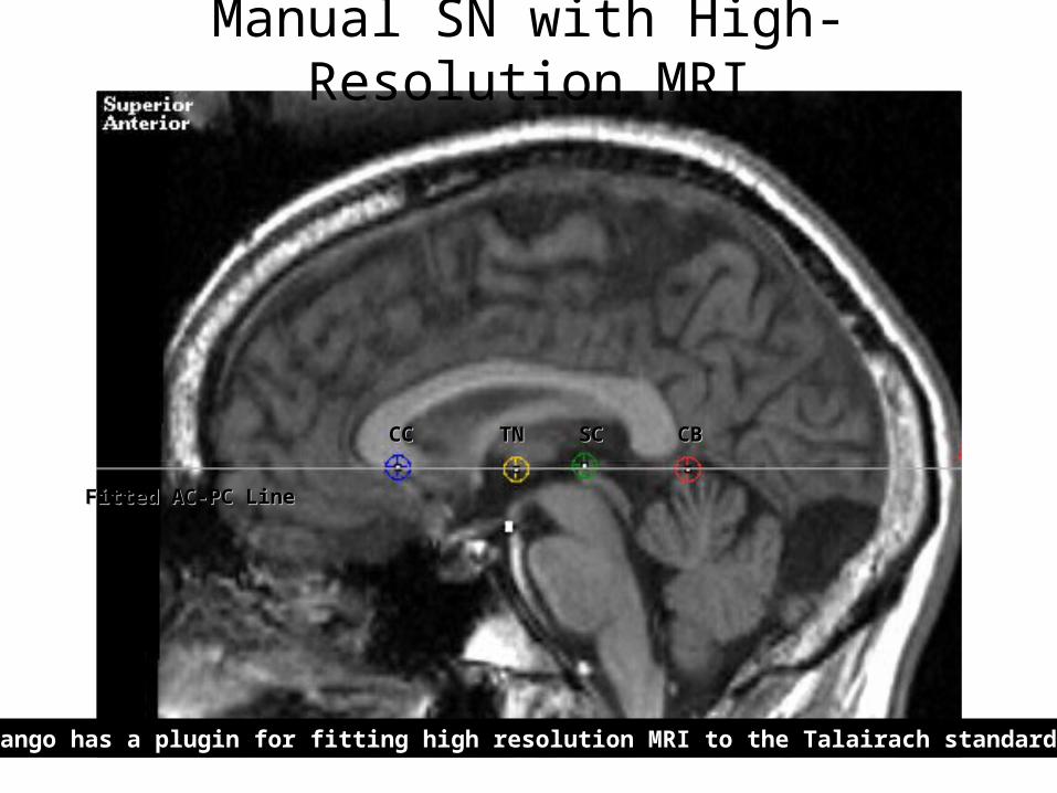
Fitted AC-PC LineFitted AC-PC Line

CCCC TNTN SCSC CBCB

Manual SN with High-Resolution MRI

Mango has a plugin for fitting high resolution MRI to the Talairach standard.Mango has a plugin for fitting high resolution MRI to the Talairach standard.

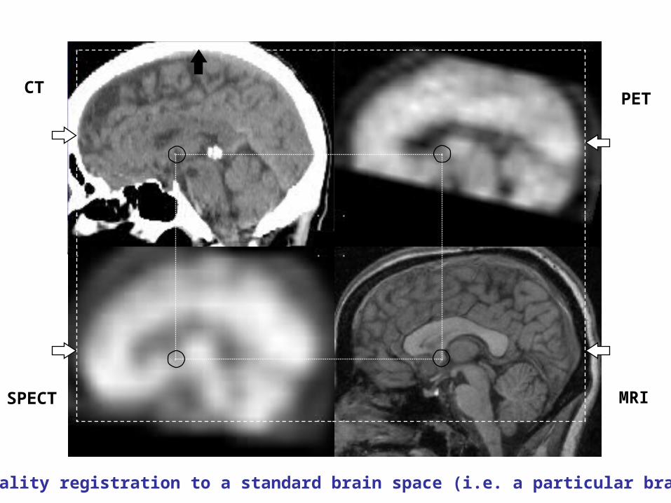
PET

SPECT MRI

CT

Multi-modality registration to a standard brain space (i.e. a particular brain atlas).

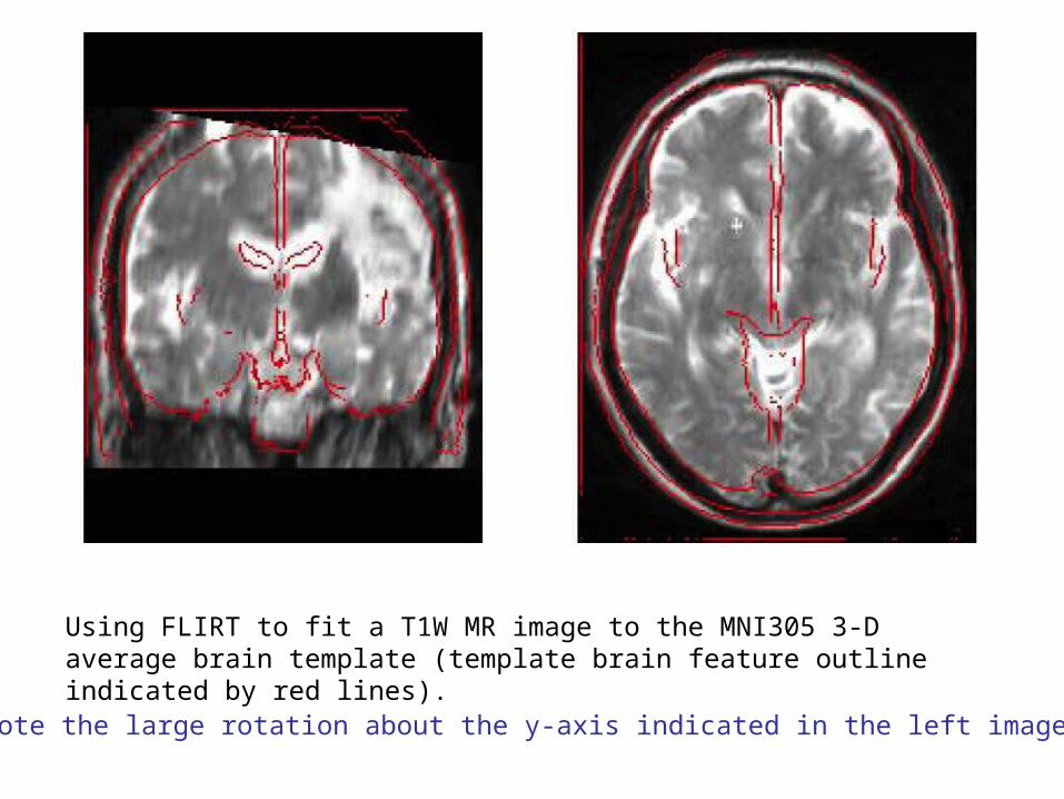
Using FLIRT to fit a T1W MR image to the MNI305 3-D average brain template (template brain feature outline indicated by red lines).

Note the large rotation about the y-axis indicated in the left image.

Atlas Based Registration of fMRI

MNI152 structural brain template is average of 152 3-D T1W images after affine registration.

MNI152structuralEPI

M1 M2

M= [M2][M1]

What is a 7 DOF transform?All three scales are identical to correct for possible differences in spatial calibrations.

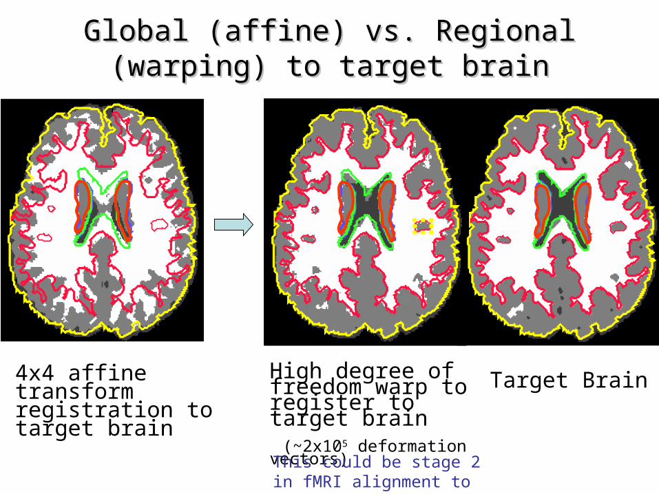
Global (affine) vs. Regional (warping) to target Global (affine) vs. Regional (warping) to target brainbrain

4x4 affine transform registration to target brain

High degree of freedom warp to register to target brain (~2x105 deformation vectors)

Target Brain

This could be stage 2 in fMRI alignment to atlas.

1

43

2

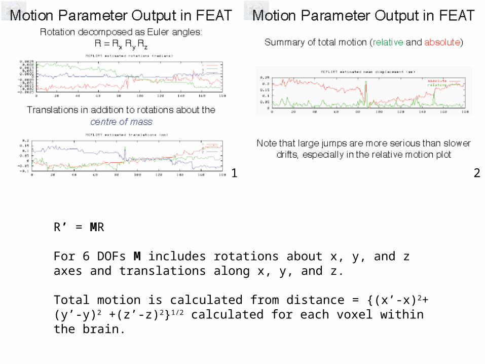
R’ = MR

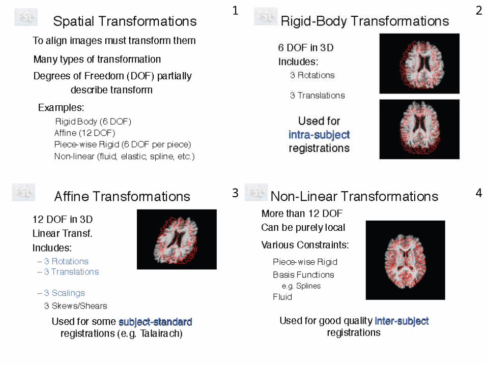
For 6 DOFs M includes rotations about x, y, and z axes and translations along x, y, and z.

Total motion is calculated from distance = {(x’-x)2+ (y’-y)2 +(z’-z)2}1/2 calculated for each voxel within the brain.

1 2

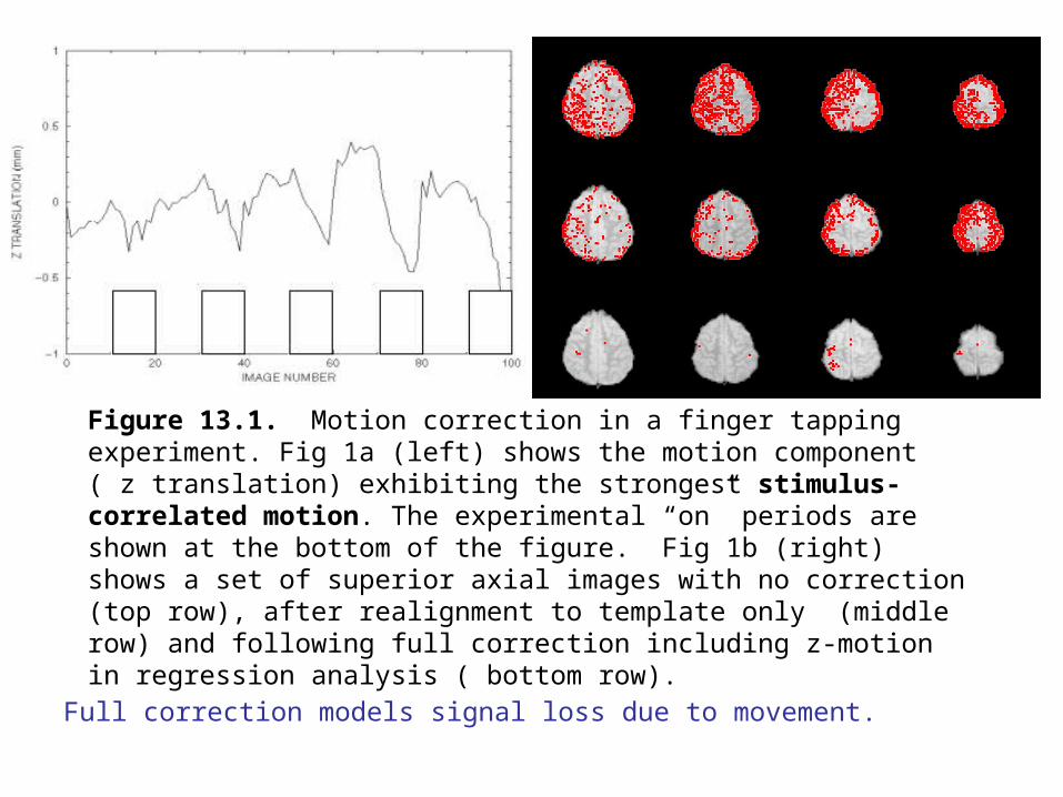
Figure 13.1. Motion correction in a finger tapping experiment. Fig 1a (left) shows the motion component ( z translation) exhibiting the strongest stimulus-correlated motion. The experimental “on” periods are shown at the bottom of the figure. Fig 1b (right) shows a set of superior axial images with no correction (top row), after realignment to template only (middle row) and following full correction including z-motion in regression analysis ( bottom row).

Full correction models signal loss due to movement.

Figure 13.2. Motion correction in a visual stimulation experiment. Fig 2a (left) shows the motion component ( z translation) exhibiting the strongest stimulus-correlated motion. The experimental “on” periods are shown at the bottom. Fig 2b (right) shows a set of superior axial images with no correction (top row), after realignment only (middle row) and following full correction( bottom row)

Figure 13.3. Two slices from a group activation map ( n=6) in schizophrenic patients before ( upper row) and after (lower row) group correction for subject motion.

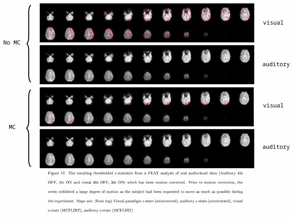
No MC

MC

visual

visual

auditory

auditory

http://www.fmrib.ox.ac.uk/fsl/