Louisiana State UniversityLSU Digital Commons

LSU Doctoral Dissertations Graduate School

2004

Statistical models and genetic evaluation ofbinomial traitsJose Lucio GuerraLouisiana State University and Agricultural and Mechanical College, jguerr2@lsu.edu

Follow this and additional works at: https://digitalcommons.lsu.edu/gradschool_dissertations

Part of the Animal Sciences Commons

This Dissertation is brought to you for free and open access by the Graduate School at LSU Digital Commons. It has been accepted for inclusion inLSU Doctoral Dissertations by an authorized graduate school editor of LSU Digital Commons. For more information, please contactgradetd@lsu.edu.

Recommended CitationGuerra, Jose Lucio, "Statistical models and genetic evaluation of binomial traits" (2004). LSU Doctoral Dissertations. 3032.https://digitalcommons.lsu.edu/gradschool_dissertations/3032

STATISTICAL MODELS AND GENETIC EVALUATION OF BINOMIAL TRAITS

A Dissertation

Submitted to the Graduate Faculty of the Louisiana State University and

Agricultural and Mechanical College in partial fulfillment of the

requirements for the degree of Doctor of Philosophy

in

The Interdepartmental Program in Animal and Dairy Sciences

by José Lúcio Lima Guerra

B.S., Louisiana State University, 1998 M.S., Louisiana State University, 2000

August 2004

ii

Dedication

This manuscript is dedicated to the memory of my mother who unfortunately was

taken from this world before the completion of this degree. Her life was an example of

how hard work and strong belief could make all things possible. She always had faith in

me and believed that I could do anything I set my mind to. To Maria Magnolia Lima

Guerra (March, 2004).

iii

Acknowledgements

I would like to express my gratitude to my major professor Dr. Donald E. Franke

for his guidance, encouragement and support in the pursuit of this degree and in the

preparation of this dissertation. It has been both a pleasure and honor to share with him

ideas and meaningful discussions on many subjects related to my research and program

of study. Also, the author wishes to express his gratitude towards his parents who have

supported him through the completion of his degree.

The author wishes to express his profound gratitude towards his wife Maria

Garcia Sole Guerra for her help and support. Also his daughters Daniela and Maria

Guerra were a great pleasure for the author during completion of this doctorate program.

Special thanks goes to his aunt, Dr. Maria da Guia Silva Lima, who has inspired

the author in the pursuit of science from an early age. Also, the author would like to

thank the staff and colleagues in the Department of Animal Sciences who contributed

towards the completion of his Ph.D. program.

The writer wishes to acknowledge the support of many friends acquired while in

Louisiana: Mert Deger, Ignacio Pellon, and Andrés Harris.

The author sends his gratitude to all his nephews and his niece. The author

wishes to send his heartfelt gratitude to his parents and brothers for always being there

for him and believing in him. Without the help of God this work would never be done.

iv

Table of Contents

Dedication ……………………………………………………………………….ii

Acknowledgments ……………………………………………………………...iii

List of Tables ……………………………………………………………….......vi

List of Figures …………………………………………………………………viii

Abstract ………………………………………………………………………....ix

Chapter I. Introduction ..………………………………………………………...1

Chapter II. Literature Review …………………………………………………..3 Response Traits in Animal Production ………………………………….3 Threshold Traits ………………………………………………………....3 The Generalized Linear Model ………………………………………….5 Statistical Models in Animal Breeding ……..…………………………...8

Estimation of Variance Components …………………………………..13 Animal vs. Sire Models for Categorical Genetic Analysis ..…………...20

Heritability Estimates for Fitness Traits ……………………………….21 Linear vs. Nonlinear Models …………………..……………………....23 The Normal Approximation to the Binomial Distribution …………….24 Crossbreeding ………………………………………………………….24 Breed Effects for Categorical Traits …………………………………...27

Chapter III. Material and Methods …….……………………………………....29 Source of the Data ………….…………………………………………..29 Management of Cattle .…………………………………………………32 Fitness Traits …………………….……………………………………..33 Statistical Models for Heritability ……....……………...………………33 Heritability Estimation ………………………………..………………..35 Estimation of Breeding Values ……………………….………………..37 Predicted Performance for Crossbreeding Systems……………..…….....37 Chapter IV. Results and Discussion ………………………….…………….....38 Family Structure of Sires and Descriptive Statistics ….…………….....38

Heritability Estimates from Linear and Non-linear Models …………...39 Comparison and Description of Expected Progeny Differences ……………………………………………………………..48 Predicted Calving Rate and Calf Survival Rate for Various Mating Systems ………………………………………………………….……..53

v

Chapter V. Summary and Implications ………………………………………..58 References ……………………………………………………………………...59

Appendix Fertility, Survival Rates and The SAS Program to Estimate Genetic Parameters ………………………………………………………….67

Vita ……………………………………………………………….…………….79

vi

List of Tables

2.1 List of distributions and link functions .…………………………………6

2.2 Heritability estimates for calving rate and calf survival ………..……...23

3.1 Mating systems and breed composition of dams over five generations .31

4.1 Cumulative distribution of sire family size …..………………………..38

4.2 Distribution of calving rate (CR) and calf survival (CS) records and mean performance by mating system and breed of sire ……………………...39

4.3 Quasi-likelihood estimates of sire component of variance (sirevar) and error

variance (error) ………………………………………………………...40

4.4 Average of 10,000 estimates from the independence chain sampling of the posterior distribution of the sire component of variance (sirevar) and error variance (error) ………………………………………………………...40

4.5 Descriptive statistics for the posterior distribution of heritability from the kernel density procedure ………………………………………….........45

4.6 The deviance and scaled deviance of the major models used to analyze

calving rate (CR) and calf survival (CS) …...………………………….47

4.7 Cumulative distribution of sire breeding values for calving rate and calf survival estimated with the logistic model ..…………………..…….....49

4.8 Cumulative distribution of sire breeding values for calving rate and calf

survival estimated with the normal model …………………………......50

4.9 Cumulative distribution of sire breeding values for calving rate and calf survival estimated with the probit model .……….…………………......50

4.10 Cumulative distribution of sire breeding values for calving rate and calf survival estimated with the transformed logistic model …………….…50

4.11 Cumulative distribution of sire breeding values for calving rate and calf survival estimated with the transformed probit model ……...…………51

4.12 Spearman rank correlation between sire EPD values for calving rate from all models ……………….………………………….………………….51

4.13 Spearman rank correlation between sire EPD values for calf survival from

all models ……………………………………………………….……..51

vii

4.14 Least squares means (LSM) for breed of sire EPDs for daughter calving rate (CR) and calf survival (CS) ..…………………………………….55

4.15 Direct and maternal breed additive and nonadditive genetic effects for calving rate and calf survival ………………………………………...56

4.16 Predicted calving rate and calf survival for major mating systems ….57

viii

List of Figures

4.1 Posterior density estimates of heritability. Calving rate estimates are to the left and calf survival estimates are to the right. From the top to the bottom the models represented are the logistic, normal, and probit. …………..42

4.2 Posterior density estimates of heritability after adjustments are applied. Calving rate estimates are to the right and calf survival estimates are to the left. From the top to the bottom the models represented are the logistic and probit. …………………………………………………………………..43

4.3. Distribution of the EPDs for calving rate (left) and calf survival (right), a normal distribution is superimposed. …………………………………..53

ix

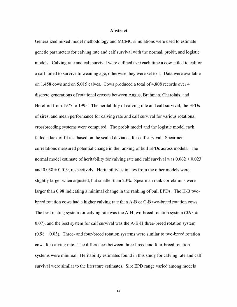
Abstract

Generalized mixed model methodology and MCMC simulations were used to estimate

genetic parameters for calving rate and calf survival with the normal, probit, and logistic

models. Calving rate and calf survival were defined as 0 each time a cow failed to calf or

a calf failed to survive to weaning age, otherwise they were set to 1. Data were available

on 1,458 cows and on 5,015 calves. Cows produced a total of 4,808 records over 4

discrete generations of rotational crosses between Angus, Brahman, Charolais, and

Hereford from 1977 to 1995. The heritability of calving rate and calf survival, the EPDs

of sires, and mean performance for calving rate and calf survival for various rotational

crossbreeding systems were computed. The probit model and the logistic model each

failed a lack of fit test based on the scaled deviance for calf survival. Spearmen

correlations measured potential change in the ranking of bull EPDs across models. The

normal model estimate of heritability for calving rate and calf survival was 0.062 ± 0.023

and 0.038 ± 0.019, respectively. Heritability estimates from the other models were

slightly larger when adjusted, but smaller than 20%. Spearman rank correlations were

larger than 0.98 indicating a minimal change in the ranking of bull EPDs. The H-B two-

breed rotation cows had a higher calving rate than A-B or C-B two-breed rotation cows.

The best mating system for calving rate was the A-H two-breed rotation system (0.93 ±

0.07), and the best system for calf survival was the A-B-H three-breed rotation system

(0.98 ± 0.03). Three- and four-breed rotation systems were similar to two-breed rotation

cows for calving rate. The differences between three-breed and four-breed rotation

systems were minimal. Heritability estimates found in this study for calving rate and calf

survival were similar to the literature estimates. Sire EPD range varied among models

x

but was less for the normal model. Predicted performance for mating systems is possible

with estimates of genetic effects.

1

Chapter I

Introduction

Calving rate and calf survival have a binomial distribution and are often called

“all or none” traits. Cows calve or they fail to calve in a specific calving season. A

newborn calf may or may not survive to weaning. These two fitness traits contribute

greatly to reproduction, arguably the most important trait in beef cattle production.

Variation in calving rate or calf survival is said to exist on an unobserved continuous

scale that becomes visible when this underlying scale crosses a threshold. Estimates of

additive genetic variance for calving rate and calf survival are relatively small compared

to phenotypic variance, resulting in heritability estimates less than 15 percent (Koots et

al., 1994; Doyle et al., 2000). Concerns when estimating heritability of binomial traits

include the correct model to use and whether to transform the binomial data to a

continuous scale.

Breeding values for growth, maternal milk, and carcass traits are printed on sire

and cow registration certificates and published by breed associations. Breeding values are

also published for scrotal circumference, a trait related to fertility, and for calving ease, a

trait related to calf survival; but no estimates of breeding value are published for cow or

sire fertility or for calf survival. One of the reasons for this situation is the relatively low

heritability estimates for calving rate and calf survival and the prediction of relatively

small breeding values with low accuracies. The majority of heritability estimates and

breeding values for fitness traits in the literature traits have been estimated from purebred

cattle data.

2

Dickerson (1970) stated that efficient production in any species depends on

reproduction and maternal ability of females and on growth of progeny. Melton (1995)

reported that reproduction of beef cattle was 3.2 times more important than growth or

carcass traits. Doyle et al. (2000) suggested that a goal of every beef cattle enterprise

should be to wean a live calf annually from each cow in the herd, which depends on

reproduction of the cow and survival of the calf.

Differences between breeds for calving rate and calf survival have been reported

(Cartwright et al., 1964; Turner et al., 1968; Williams et al., 1990). Williams et al.

(1991) demonstrated that breed direct and maternal additive and non-additive genetic

effects could be partitioned for reproductive traits and that these effects could be used to

predict mean performance for various crossbred types. Because of the importance of cow

fertility and offspring survival in beef cattle, the objectives of this study were:

1. To estimate the heritability of calving rate and calf survival using normal, logistic,

and probit models,

2. To predict sire breeding values for daughter calving rate and calf survival,

3. To predict calving rate and calf survival for various rotational crossbreeding

systems with the use of direct and maternal breed additive and non-additive

genetic effects.

3

Chapter II

Literature Review

Response Traits in Animal Production

Response traits in animal production can be expressed on a continuous scale or as

categorical traits. Production traits such as growth rate, body weight, carcass weight,

ribeye area, Warner-Bratzler shear force, etc, are generally expressed on a continuous

scale and are assumed to be normally distributed. Fitness traits such as calving rate,

calving ease, and calf survival are examples of categorical traits.

Threshold Traits

Many categorical, or threshold, traits are assumed to be under polygenic control

and random environmental effects (Falconer, 1989). Most biological traits and diseases

have this type of inheritance, often called multifactorial inheritance (Anderson and

Georges, 2004). An underlying, continuous distribution (liability) is assumed. Extensive

work has been reported on analysis of discrete data in animal breeding (Wright, 1934;

Gianola, 1982; Gianola and Foulley, 1983, and others).

Models for analyzing continuous responses are often said to be inadequate for

categorical responses (Thompson, 1979; Gianola, 1982; Koch et al., 1990; Ramizez-

Valverde et al., 2001). Generally a transformation of the categorical trait is performed or

a model for continuous data is applied to the binomial trait.

In the beginning of the twentieth century, Weinberg proposed methods to separate

genetic and environmental components of variance (Dempster and Lerner, 1950). Dr. J.

L. Lush proposed the term “heritability” for the proportion of phenotypic variance that is

due to genetic variance. Heritability that is presented today in the literature is the additive

4

heritability, that portion of the phenotypic variance due to additive genetic variance.

Most applications of the concept of heritability refer to continuously varying traits that

follow a normal distribution on the observed phenotypic scale. However, the heritability

concept can be applied to binary traits that are expressed phenotypically or observed in an

“all or none” fashion.

Wright (1934) indicated that for a discontinuous trait to be exposed, a threshold

point on the underlying continuous scale (liability scale) must be crossed. Liability is

influenced by environmental factors and by many genes that have small additive effects

(Dempster and Lerner, 1950). Wright (1934) also proposed a transformation for

discontinuous data to a continuous scale. Bliss in 1935 reintroduced Wright’s

transformation as a “probit” transformation and the name gained wide acceptance in the

scientific community (Agresti, 2002).

Environmental effects are assumed to be independent of additive genetic effects

and to be normally distributed. Gianola (1982) suggested that genetic and environmental

effects are not statistically independent on the observed binomial scale (p-scale). The

probit transformation from a binomial scale to the underlying liability scale is well

known in the animal breeding literature (Dempster and Lerner 1950; Van Vleck, 1972;

Gianola, 1982). A simulation study of this transformation was found to produce slight

overestimates of heritability when paternal half-sib data were used (Van Vleck, 1972;

Gianola, 1982).

The link between the liability and the observed scale can be accomplished with

the cumulative normal distribution function. In the case of a binomial phenotype such as

calving rate or calf survival, the average frequency of ones is the point where the

5

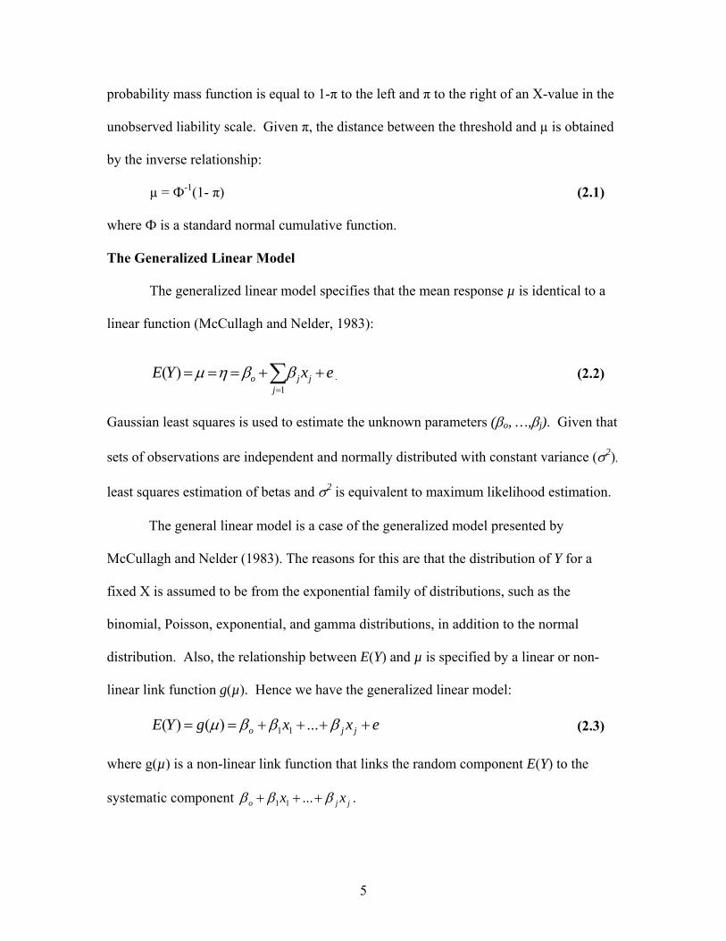
probability mass function is equal to 1-π to the left and π to the right of an X-value in the

unobserved liability scale. Given π, the distance between the threshold and µ is obtained

by the inverse relationship:

µ = Ф-1(1- π) (2.1)

where Ф is a standard normal cumulative function.

The Generalized Linear Model

The generalized linear model specifies that the mean response µ is identical to a

linear function (McCullagh and Nelder, 1983):

∑=

++===1

)(j

jjo exYE ββηµ . (2.2)

Gaussian least squares is used to estimate the unknown parameters (βo, …,βj). Given that

sets of observations are independent and normally distributed with constant variance (σ2),

least squares estimation of betas and σ2 is equivalent to maximum likelihood estimation.

The general linear model is a case of the generalized model presented by

McCullagh and Nelder (1983). The reasons for this are that the distribution of Y for a

fixed X is assumed to be from the exponential family of distributions, such as the

binomial, Poisson, exponential, and gamma distributions, in addition to the normal

distribution. Also, the relationship between E(Y) and µ is specified by a linear or non-

linear link function g(µ). Hence we have the generalized linear model:

exxgYE jjo ++++== βββµ ...)()( 11 (2.3)

where g(µ) is a non-linear link function that links the random component E(Y) to the

systematic component jjo xx βββ +++ ...11 .

6

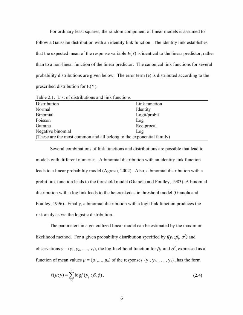
For ordinary least squares, the random component of linear models is assumed to

follow a Gaussian distribution with an identity link function. The identity link establishes

that the expected mean of the response variable E(Y) is identical to the linear predictor, rather

than to a non-linear function of the linear predictor. The canonical link functions for several

probability distributions are given below. The error term (e) is distributed according to the

prescribed distribution for E(Y).

Table 2.1. List of distributions and link functions Distribution Link function Normal Identity Binomial Logit/probit Poisson Log Gamma Reciprocal Negative binomial Log (These are the most common and all belong to the exponential family) Several combinations of link functions and distributions are possible that lead to

models with different numerics. A binomial distribution with an identity link function

leads to a linear probability model (Agresti, 2002). Also, a binomial distribution with a

probit link function leads to the threshold model (Gianola and Foulley, 1983). A binomial

distribution with a log link leads to the heteroskedastic threshold model (Gianola and

Foulley, 1996). Finally, a binomial distribution with a logit link function produces the

risk analysis via the logistic distribution.

The parameters in a generalized linear model can be estimated by the maximum

likelihood method. For a given probability distribution specified by f(yi ;βj, σ2) and

observations y = (y1, y2, . . ., yn), the log-likelihood function for βj and σ2, expressed as a

function of mean values µ = (µ1,…, µn) of the responses {y1, y2, . . . , yn}, has the form

),;(log);(1

φβµ i

n

iyfy ∑

=

=l . (2.4)

7

The maximum likelihood estimates of the parameters βj can be derived by an iterative

weighted least-square procedure as demonstrated by Nelder and Wedderburn (1972).

Detailed information about the iterative algorithm and asymptotic properties of the

parameter estimates can be found in McCullagh and Nelder (1983).

Analogous to the residual sum of squares in linear regression, the goodness-of-fit

of a generalized linear model can be measured by the deviance (D),

D = );(^

fyl µ - );(

^

ryl µ (2.5)

where );(^

fyl µ is the maximum likelihood achievable for an exact fit (full model) and

);(^

ryD µ is the log-likelihood function calculated for the estimated parameters βj

(reduced model). The full model has as many parameters as there are observations, hence

a lack of fit test for a model against the data can be composed based on likelihood

methodology. The difference in the likelihoods between the full and reduced model has

as many degrees of freedom as the numbers of observations in the data minus the number

of parameters in the reduced model. The deviance can be used as a 2χ statistic to test the

goodness of fit of a model (Littell et al., 1996; Royall, 2000). Generalized linear models

also have an extra-dispersion parameter ө. This extra-dispersion parameter is the

deviance divided by the number of observations. Ideally ө = 1, but if it is substantially

different from 1 the deviance should be adjusted by the ө (Littell et al., 1996). This

measure is called scaled-deviance. The deviance and scaled deviance are used in a

similar manner.

8

The deviance or the scaled deviance can be also used to compose a likelihood

ratio test for nested models. The deviance of several cases of the generalized linear

model (logistic, Poison, and probit) can be calculated with PROC GENMOD (SAS) and

the GLIMMIX macro (SAS). The generalized linear model can be expanded into a

generalized mixed model. The generalized mixed model has conditional interpretations

and for this reason is said to be a subject specific model instead of a population average

model. The probit-normal and logistic-normal models are the most popular forms of the

generalized mixed models; both models are non-linear (Agresti, 2002).

Statistical Models in Animal Breeding

The approach that put together the principles of the generalized linear model,

quasi-likelihood, and the idea of random effects was very important for statistical

modeling of binary data (Breslow and Clayton, 1993). Quasi-likelihood methodology is

used by computer software to fit the non-linear cases of the generalized linear model in

order to model binary data (Weddenburn, 1974; McCullagh and Nelder, 1983).

It is difficult to compare models for binary data with models for continuous data

because the models are in different numeric scales (Littell et al., 1996; Matos, 1997b).

Different mathematical models refer to models with different link functions. Different

distribution functions are assumed for the response trait and different link functions

contribute to the problem of comparing mathematical models in different numeric scales.

The logistic, normal, and threshold models are the most frequent mathematical models

used in animal breeding. These models have different structural components. Different

structural components account for different sources of variation and lead to different

biological models such as permanent and temporary environmental effects, e.g. the

9

repeatability model, sire model, and animal model. Statistical models refer to different

sets of assumptions such as Poisson regression, logistic regression, and negative binomial

regression. However, there are statistical models that produce heritability estimates that

have no biological interpretation. Littell et al. (1996) cited the logistic model as an

example of this. On the other hand the logistic model has some specific applications in

human genetics and in molecular genetics because its numerics are in the logistic scale,

e.g. the logarithmic of the odds scale or the lod-score. The lod-score is used to imply

linkage of molecular markers with a phenotype (Weir, 1996; Page et al., 1998). Logistic

regression coefficients for fixed and random effects are in the lod-scale (logistic scale)

and these values could be used to imply linkage (association) of a genetic or

environmental factor with a phenotype. The estimated values have to be inside a range set

for statistically detecting linkage. If the lod-score of a genetic factor or environmental

factor is above 3 or below -2 the linkage or association is said to be statistically

significant (Weir, 1996; Page et al., 1998). Lod-scores below -2 indicate association with

the absence of the phenotype of interest. Lod-scores larger than 3 suggest there is

association with the phenotype of interest. For a fertility trait, large positive values are

associated with cows that calve and large negative values are associated with cows failing

to calve.

The traditional threshold model (probit) postulates that a linear model with a non-

linear relationship between the observed and underlying scale describes the underlying

variable called liability (Gianola and Foulley, 1983). Thus, we have a generalized linear

model linked to the binomial trait with a probit link function (GLMMp). The GLMMp is

equivalent to the Maximum A Posteriori, or MAP procedure suggested by Gianola and

10

Foulley (1983). The GLMMp can be implemented in SAS with the help of the

GLIMMIX macro.

In a regular liner model the variance is assumed to be independent of the mean

since the Gaussian distribution is used. This is not true when the response is binary. The

variance of a binary trait is a function of the average. So, the assumed initial conditions

or the statistical model used in linear modeling do not describe properly the nature of

binary data. However, from probability theory it is known that under asymptotic

conditions the Gaussian (normal) distribution approximates the binomial distribution

(central limit theorem).

An important step when fitting linear or non-linear models to animal breeding

data is the use of pedigree information. This information is used to build the additive

genetic covariance, or A matrix (Wright, 1922). The additive genetic covariance matrix

expresses the genetic relationship between individuals (Covij) (off-diagonal) and of an

individual with itself (Covii) (main-diagonal). The additive genetic covariance matrix is

also called a numerator relationship matrix. It is symmetrical and its diagonal element

for animal i (Covii) is equal to 1 + Fi, where Fi is the inbreeding coefficient of animal i

(Wright, 1922). The off-diagonal elements are equal to Covij, the numerator for the

genetic relationship coefficient equation, thus the name numerator matrix is derived from

this property. The diagonal element represents twice the probability that two gametes

taken at random from animal i will carry identical alleles by descent.

The algorithm to include all the pedigree information, heritability, and some

known fixed sources of variation into ranking of sires based on the sire’s genetic merit

was proposed by Henderson (1952). An easy strategy for finding the inverse of the

11

relationship matrix was also developed by Henderson (1976). The A matrix is then

incorporated into mixed model equations which when solved yield animal breeding

values (Henderson, 1984). The solutions for the sires are the sire expected progeny

differences (EPDs). Expected Progeny Differences may be used to estimate how future

progeny of a sire will compare to progeny of other sires within a population. Expected

Progeny Differences are expressed as deviations from the population average. When

sires are unrelated, the model reduces to simply assuming sire as a random component in

statistical software such as SAS plus fixed sources of variation. Henderson’s procedure

to estimate random and fixed effects at the same time has a valid theoretical basis

(Harville, 1976). The methodology is commonly known as mixed model estimation

(MME) because fixed effects (herd, year, and breed) and random effects (animal,

temporary and permanent environmental effects) can be estimated simultaneously. The

procedure has gained acceptance and has been applied to a wide variety of statistical

problems.

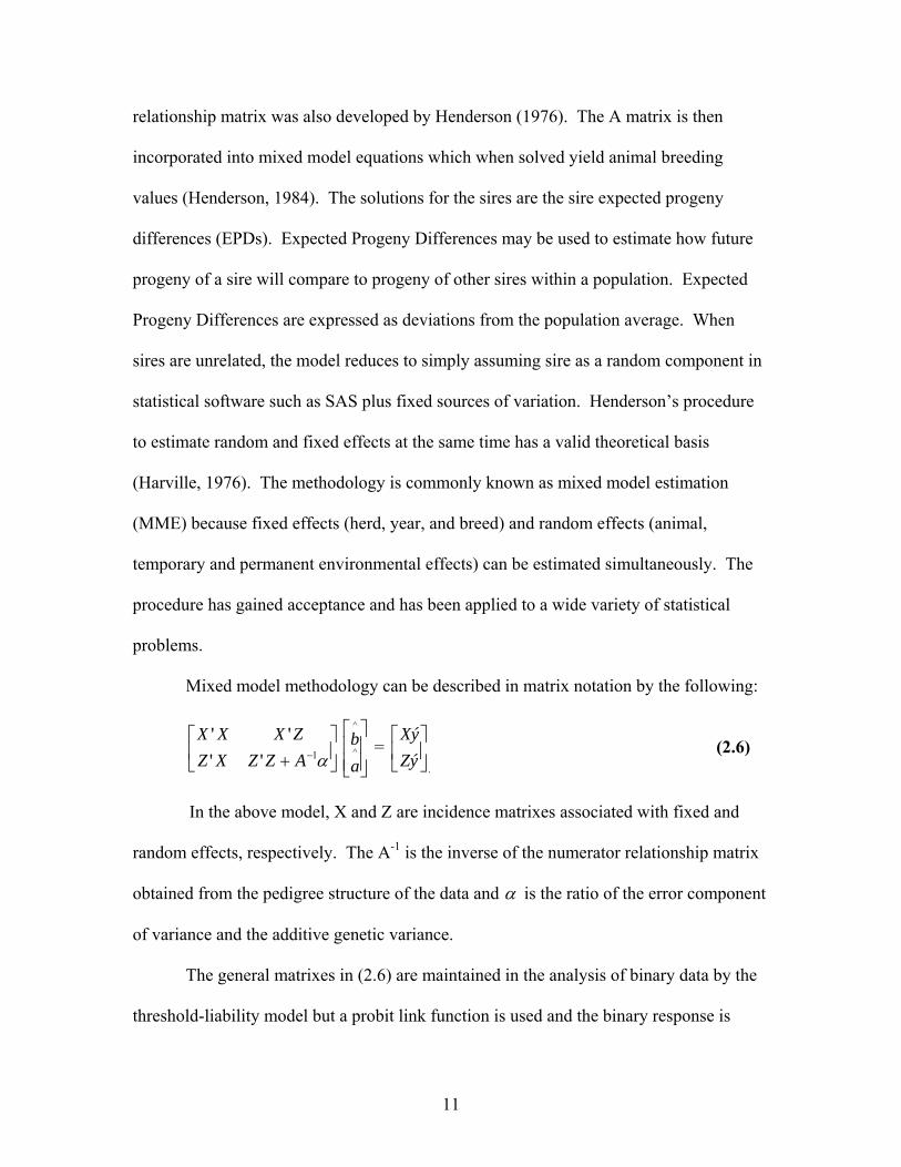
Mixed model methodology can be described in matrix notation by the following:

⎥⎦

⎤⎢⎣

⎡+ − α1''''AZZXZZXXX

⎥⎥⎦

⎤

⎢⎢⎣

⎡^

^

ab =

.⎥⎦

⎤⎢⎣

⎡ZýXý

(2.6)

In the above model, X and Z are incidence matrixes associated with fixed and

random effects, respectively. The A-1 is the inverse of the numerator relationship matrix

obtained from the pedigree structure of the data and α is the ratio of the error component

of variance and the additive genetic variance.

The general matrixes in (2.6) are maintained in the analysis of binary data by the

threshold-liability model but a probit link function is used and the binary response is

12

correctly assumed to follow a binomial distribution (Wright, 1934; Gianola, 1982;

Gianola and Foulley, 1983). The residual variance is not known hence it is assumed to be

1 (Heringstad et al., 2003). One of the reasons to use the probit 1, e.g. setting the residual

variance equal to 1, is convenience (Lush, 1948).

When a logistic model is used, a correction factor of pi-squared divided by 3 is

used because this is assumed to be the variance of a logistic distribution (Southey et al.,

2003). However, this is not the correct form of the variance of the logistic distribution.

The form of the variance is pi-squared multiply by b squared divided by 3; b is the

standard deviation of the logistic distribution which is assumed to be 1 (Southey et al.,

2003). The logistic model in its original logit scale should not be used to estimate

heritability since its real basis is difficult to interpret (Littell et al., 1996). Nowadays the

assumptions of fixed residual variances can be relaxed because of the quasi-likelihood

algorithm (McCullagh and Nelder, 1983).

The practice of using correction factors in non-linear models could be equivalent

to transforming a transformation when undesirable results are achieved. Non-linear

models have specific usage without the need of correction factors. When lod-scores are

used in molecular genetics, results are interpreted without a correction factor for the

observed logit, e.g. lod-score scale (Page et al., 1998). The probit model assumes an

underlying normal distribution. Its values are in the z-score scale, e.g. in the cumulative

normal scale. However, the two models have different interpretations as the logit is used

to imply linkage and the probit is used in the estimation of the underlying liability of a

trait.

13

Estimation of Variance Components

In statistical terminology, the second moment statistics are variances and

covariances. It is assumed that second moment statistics (variances) are less reliable than

the first moment statistics (averages). Since many statistics used in animal genetics are

computed from the variances and covariances (heritability, genetic correlation and

repeatability), these statistics should be estimated with large samples and with

appropriate analytical tools (statistical algorithms). There are currently several methods

to estimate (co)variances, and the search of better algorithms to accurately estimate

(co)variances has been an important area in animal breeding. Some of the common

methods for variance component estimation include the traditional analysis of variance

(ANOVA) methods such as Henderson’s methods 1, 2, 3, and 4, minimum-norm-

quadratic unbiased estimation (MINQUE), maximum likelihood estimation (ML),

restricted maximum likelihood estimation (REML) and derivative free restricted

maximum likelihood estimation (Harville, 1977; Henderson, 1984; Meyer, 1989; 1991).

Estimation of variance components in ANOVA is performed with ordinary least

squares. The estimated least square mean from the data is set to be equal to the derived

expression of their expected values. The variance components are then derived as if an

equation system is being solved. The traditional analysis of variance requires the sample

data to be balanced, e.g. similar sample sizes among the fixed effects. Unfortunately,

field data are often unbalanced. On the other hand, ML and REML estimators do not

require the data to be in a specific design or have balanced fixed effects.

Restricted maximum likelihood (REML) was introduced by Thompson (1962)

and expanded by Patterson and Thompson (1971). It has been reported that REML is

14

marginally sufficient, consistent, efficient, and asymptotically normal (Harville, 1977).

These statistical properties lead to utilization of all information in the best way possible.

The past decade has seen an increase in the usage of restricted maximum likelihood

(REML) as the method of choice for analyzing genetic data. In the case of REML, the

increased level of computing power is not the major force behind the popularization, but

rather the increased number of algorithms that benefit from specific data structure and

numerical techniques such as sparse matrix algorithms (Meyer, 1989). The restricted

maximum likelihood methodology partitions the likelihood function into two parts. One

part does not contain fixed effects and it works on the likelihood of linear functions of the

data vector. These functions are called error contrasts or the part of the likelihood

function that is independent of the fixed effects (Patterson and Thompson, 1971). The

main difference between ML and REML is that when REML is used it utilizes the

likelihood of the linear function instead of the likelihood of the vector of observations.

The major advantage of REML is that negative components of variance are not possible

while in maximum likelihood a negative component is possible. This has been referred

to as a theoretical prior and it was implied that REML is naturally a Bayesian method of

estimation (Gianola and Fernando, 1986).

In non-linear models there is an association (dependence) between the marginal

expectation of the data and the variance of the random effects (Zeger et al., 1988; Moreno

et al., 1997). This conclusion suggests that the estimators of fixed effects and the

variance components are not asymptotically orthogonal, e.g. the fixed and random effects

are not independent, even in large samples. On the other hand this problem does not exist

in the Gaussian model (Moreno et al., 1997).

15

The nonconjugate Bayesian analysis of variance components (NBVC) was

described by Wolfinger and Kass (2000). The nonconjugate Bayesian analysis of

variance components estimates the posterior distribution of the parameters (heritability)

with the independence chain algorithm that employs Markov Chain Monte Carlo

(MCMC) methodology. The nonconjugate Bayesian analysis of variance uses non-

informative priors, e.g. priors that reflect ignorance. These priors have been investigated

extensively (Jeffreys, 1961). Thus, for a question of invariance and for the sake of

inference with accepted frequentist characteristics, Jeffreys’ priors are used in the NBVC

(Wolfinger and Kass, 2000). Jeffreys’ rule for determining a prior is to use a prior that is

equivalent to the square root of the determinant of the Fisher information matrix. The

Fisher information matrix is the observed inverse of the asymptotic variance matrix

evaluated at the final covariance parameter estimate, e.g. at convergence. The Fisher

information matrix is 2 times the Hessian matrix and the elements of the Hessian matrix

are second derivatives of a gradient function. In a surface grid of X and Y a gradient

function would be associated with the slope of the surface toward a maximum. This

technique has an application in the statistical concept of maximum likelihood.

The nonconjugate Bayesian analysis of variance components have advantages

over regular Bayesian inference that uses a Gibbs sampling scheme. First, NBVC

methodology is easy to use and is available in SAS software. Second, the NBVC

methodology in SAS minimizes demands made on the user to monitor the simulation, e.g.

it automatically performs a statistical control over the sampling algorithm with a constant

check of the posterior distribution. This type of check was called convergence

diagnostics (Heringstad et al., 2001; 2003). The diagnostic procedure was intended to

16

guarantee a ± 0.05 accuracy. The same level of accuracy was adopted in the NBVC by

Wolfinger and Kass (2000) and Heringstad et al. (2001; 2003). The NBVC produces a

random sample of variance components given the initial model (logistic, normal, or

threshold). This procedure is repeated independently ten thousand times and the first and

second moment statistics computed and stored. This new dataset is a random sample of

the posterior distribution of variance components, which are used to estimate heritability.

This sampling scheme is referred as an independent chain in MCMC terminology

(Wolfinger and Kass, 2000). Wolfinger and Kass (2000) performed a kernel density

estimation of the random sample generated by the MCMC methodology. The kernel

density estimation was performed with PROC KDE in SAS. PROC KDE approximates a

hypothesized probability density function of observed data. A known density function

(kernel) is averaged across the observed data points. The result is a smooth

approximation of the hypothesized probability density function (variance components

ratio: heritability). PROC KDE uses a Gaussian function as the kernel (SAS, 2000). The

NBVC estimation proposed by Wolfinger and Kass (2000) is a MCMC generation of a

random sample of variance component estimates given the observed data. These

estimates are used in a kernel density estimation to infer the density of the posterior mass

function of variance components or of the genetic parameters, such as heritability. In

animal science literature MCMC algorithms are referred to as Monte Carlo simulation

(Phocas and Laloe, 2003). Finally, NBVC allows one without enough statistical

information to benefit from the Bayesian inference. Bayesian inference is useful to

estimate confidence intervals for variance components and for ratios of variance

components such as heritability. The statistical methodology used in the NBVC is an

17

alternative to restricted maximum likelihood estimation of variance components

(Wolfinger and Kass, 2000). The Monte-Carlo simulation methods in animal breeding

have replaced normal approximations of a posterior distribution by numerical integration

(Matos et al., 1993).

Gibbs sampling is also a MCMC algorithm that is used in animal breeding

studies. Gibbs sampling is difficult to implement if the full posterior distributions of

unbalanced datasets have to be simulated (Wolfinger and Kass, 2000). The hypothesized

posterior distribution of the parameter of interest needs to be spherical, symmetrical, and

sharp to be considered precise (Bernardo and Smith, 2002).

Resampling has been used to generate the posterior distribution of variance

components in several studies. Evans et al. (1999), Doyle et al. (2000), and Eler et al.

(2002) used resampling and found that the resulting posterior distributions of heritability

for heifer pregnancy were not spherical, symmetrical, or sharp. Heringstad et al. (2001;

2003) used Gibbs sampling and found spherical, symmetrical, and sharp posterior

distributions. Donoghue et al. (2004) used Gibbs sampling but did not report the shape of

posterior distribution. Heringstad et al. (2001; 2003) investigated clinical mastitis. The

trait of interest in the study by Donoghue et al. (2004) was fertility by artificial

insemination. Both of the traits were binomially distributed.

Method R is a recent method to estimate variance components. The fundamental

principle of method R is that as the amount of information between analysis increases,

the covariance between the predictions made by each analysis remains constant and

equals the variance of the previous (less accurate) prediction. Method R is used with

18

large data sets. Method R is often used with resampling (Evans et al., 1999; Doyle et al.,

2000; Eler et al., 2002).

Statistical models to estimate the variance components of threshold traits must be

carefully evaluated. In binary responses the relative input from non-additive genetic

variance compared with the total genetic variance on the observed scale increases as

heritability increases and as the frequency of the observed binary response deviates from

50 percent (Dempster and Lerner, 1950). Thus, the results are not independent of initial

conditions. The variance of the binomial distribution is a function of the mean.

Heritability will chance as the frequency of the binary trait of interest changes; since

heritability is a function of the variance components. The additive variance for

individuals in the threshold scale may not be estimable. Even though individuals may

have high genetic value (high liability values), this cannot be observed since only the p-

scale is observed, and it is limited by the all or none expression of the binomial

phenotype (Robertson and Lerner, 1949). Environmental sources of variation could go

unnoticed in the p-scale because this scale obscures the finer degrees of measurable

variation. The natural solution for these problems is to transform the p-scale and estimate

variance components in the transformed scale.

Dempster and Lerner (1950) recommended an adjustment that uses the height of

the ordinate of the normal distribution at the threshold value that separates the binary data

into the 1 or 0 groups. This adjustment simply proposes the multiplication of heritability

by (p(1-p))/z2 where z is the height of the ordinal estimated with the mass function of the

normal distribution at z and z is the z-score associated with the probability (p) from the

binary data being analyzed. This transformation was determined to be applicable for

19

half-sib designs but not very efficient in parent-offspring designs (Van Vleck, 1972). A

numerical example of how to use these formulae was given by Milagres et al. (1979).

The model described above is the probit, or threshold model. Non-linear models in

animal breeding that take into account the binary nature of the data were introduced in

order to estimate heritability based on an underlying normal scale because of the

difficulties associated with the p-scale (Gianola and Foulley, 1983). In spite of their

desirable theoretical properties, non-linear models have not become widely implemented

for genetic analysis because they are more complicated and computationally more

demanding. Non-linear models are used in animal breeding as replacements for linear

models (Meijering and Gianola, 1985; Matos et al., 1997a; Abdel-Azim et al., 1999;

Varona et al., 1999).

Foulley (1992) suggested that heritability calculated from the underlying normal

distribution (liability) should not be used for computing expected rates of genetic

improvement for binomial traits. Categorical traits are apparently more responsive to

family selection than individual selection (Falconer, 1989). Also, because of an

asymmetrical response to section (Foulley, 1992), heritability of binary traits is more

elusive regardless of the statistical model used. The estimation of heritability in the

underlying scale may ultimately establish that the p-scale can be used satisfactorily and

could lead to realistic results from family selection (Robertson and Lerner, 1949). The

probit transformation can be thought of as a diagnostic for heritability in the p-scale and

as a tool to determine what variables influence the underlying unobserved stochastic

process (liability) of phenotypical expression of a binary trait. Higher estimates of

heritability in the underlying scale could mean that there are environmental factors that

20

influence the binary trait and they are not accounted for in the statistical analysis

(Falconer, 1965).

Genetic evaluation of sires assumes that the variance components are known and

that heritability estimates are available, even if incorrect (Gianola and Foulley, 1986).

The empirical true BLUP cannot be calculated since we actually never know the true

variance components. A good statistical model for animal evaluation should produce

theoretically correct results. It would not be reasonable to use a statistical model that

produces confidence intervals for heritability whose interval includes values greater than

one or smaller than zero. Some theoretical criteria can be established to compare models

that are not in the same numeric scale. The posterior distribution of heritability between

two traits can be compared regardless of the numerical scale that is being used to estimate

this statistic. However comparing the heritability from different scales is more difficult

because these scales represent different numerical realities that are different and may be

incomparable (Phocas and Laloe, 2003). However, the density of posterior distributions

can be compared, avoiding the problem of using the heritability estimates from these

various scales as criteria. Heringstad et al. (2001; 2003) considered posterior

distributions that were sharper, more spherical, and more symmetrical as more precise.

Animal versus Sire Models for Categorical Genetic Analysis

Moreno et al. (1997) discussed the inadequacy of the animal model to estimate

genetic parameters such as heritability for traits on the binomial scale. Several authors

recommended using a sire model rather than an animal model to estimate genetic

parameters for binomial traits (Heringstad et al., 2003; Phocas and Laloe, 2003). Using

84,820 observations from the American Gelbvieh Association, Ramizez-Valverde et al.

21

(2001) compared linear sire models with linear animal models and non-linear sire models

with non-linear animal models under several scenarios. When the progeny number per

sire was less than 50, the use of a threshold sire model decreased the overall predictive

ability by 2%. As the number of progeny per sire increased, the difference in predictive

ability between a sire and an animal model and between linear and non-linear models

became nonexistent. Other studies estimating genetic parameters found no clear

incentive for using non-linear models over linear models (Varona et al., 1999). However,

the use of multivariate models may be more useful than a non-linear model to estimate

genetic parameters (Verona et al., 1999; Ramizez-Valverde et al., 2001).

Heritability Estimates for Fitness Traits

Koots et al. (1994) reported adjusted averages of heritability from a number of

published estimates. The heritability estimates reviewed by Koots et al. (1994) were

obtained using a probit model. Adjusted averages were considered better estimates than

unadjusted averages. Koots et al. (1994) reported the average adjusted heritability of

calving rate (n = 24) and calf survival (n = 4) to be 0.170 ± 0.015 and 0.06 ± 0.009,

respectively. Koots et al. (1994) concluded that heritability estimates for fitness traits

were limited and were generally low (0.00 – 0.20). They reported the average heritability

of heifer pregnancy to be 0.05 ± 0.01. Snelling et al. (1996) estimated the heritability of

heifer pregnancy to be 0.21 ± .11. Doyle et al. (1996) estimated the heritability of heifer

pregnancy to be 0.30 (no standard errors were reported). The higher heritability values

recently reported for heifer pregnancy may be attributed to the analytical procedures

adopted which may or may not be more appropriate for handling categorical data

(Snelling et al., 1996). Evans et al. (1999) estimated heritability of heifer pregnancy to

22

be 0.138 ± 0.080. Doyle et al. (2000) estimated heritability of heifer pregnancy,

subsequent rebreeding, and of a cow’s ability to stay in the herd to be 0.270 ± 0.170,

0.170 ± 0.013, and 0.090 ± 0.008, respectively. Eler et al. (2002) estimated heritability

for heifer pregnancy to be 0.570 ± 0.010. Also, a confidence interval was estimated to be

0.410 – 0.750. The heritability of heifer pregnancy should be higher than the heritability

of calving rate in mature cows because heifers that do not calve are often culled after two

subsequent failures. Culling non-fertile females reduces the genetic variation for fertility

(Evans et al., 1999).

A new trend for analysis of binomial traits such as fertility is to combine one or

more continuous traits with the fertility trait in a multivariate analysis. This is referred as

continuous measures of fertility (Donoghue et al., 2004). Martinez et al. (2003) used a

data set with 7,003 records and reported heritability estimates for pregnancy status

following the first breeding season (PR1), calving status following the first breeding

season (CR1), and weaning status following the first breeding season (WR1). In this

study, the estimates of heritability for PR1, CR1, and WR1 on the observed multivariate

scale were 0.14, 0,14, and 0.12 respectively. Using data from the Brazilian institute of

Zootecnology in the Sertãozinho Experimental Station, heritability was estimated in the

multivariate scale for overall calving success (CS), calving success at the first mating

(CS1), and calving success of the second mating given that the heifer calved during the

first mating opportunity (CS2). The number of observations associated with CS, CS1,

and CS2 were 947, 926, 601 and the heritability estimates on the multivariate observed

scale were 0.11 ± 0.03, 0.04 ± 0.06, and 0.10 ± .07 respectively (Mercadante et al., 2003).

The correlated trait used by Mercadante et al. (2003) was yearling weight. Heritability

23

estimates reported by Mercadante et al. (2003) and Martinez et al. (2003) were similar to

the weighted average heritability estimates reported by Koots et al. (1994). Thus,

heritability estimates of binary traits in the multivariate normal scale (continuous

heritability) appear to be in same range as the univariate estimates of heritability using a

probit model. Some of the heritability estimates for cow fertility reported in the literature

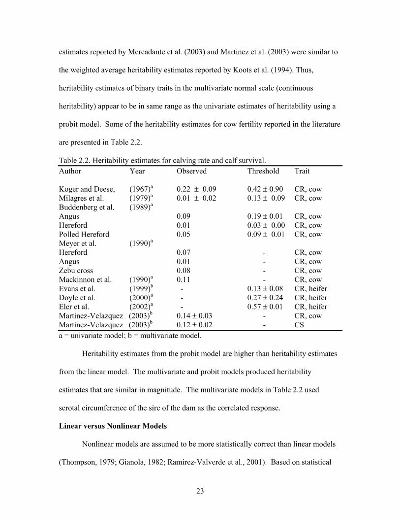
are presented in Table 2.2.

Table 2.2. Heritability estimates for calving rate and calf survival. Author Year Observed Threshold Trait Koger and Deese, (1967)a 0.22 ! 0.09 0.42 ! 0.90 CR, cow Milagres et al. (1979)a 0.01 ! 0.02 0.13 ! 0.09 CR, cow Buddenberg et al. (1989)a Angus 0.09 0.19 ! 0.01 CR, cow Hereford 0.01 0.03 ! 0.00 CR, cow Polled Hereford 0.05 0.09 ! 0.01 CR, cow Meyer et al. (1990)a Hereford 0.07 - CR, cow Angus 0.01 - CR, cow Zebu cross 0.08 - CR, cow Mackinnon et al. (1990)a 0.11 - CR, cow Evans et al. (1999)b - 0.13 ! 0.08 CR, heifer Doyle et al. (2000)a - 0.27 ! 0.24 CR, heifer Eler et al. (2002)a - 0.57 ! 0.01 CR, heifer Martinez-Velazquez (2003)b 0.14 ! 0.03 - CR, cow Martinez-Velazquez (2003)b 0.12 ! 0.02 - CS a = univariate model; b = multivariate model.

Heritability estimates from the probit model are higher than heritability estimates

from the linear model. The multivariate and probit models produced heritability

estimates that are similar in magnitude. The multivariate models in Table 2.2 used

scrotal circumference of the sire of the dam as the correlated response.

Linear versus Nonlinear Models

Nonlinear models are assumed to be more statistically correct than linear models

(Thompson, 1979; Gianola, 1982; Ramirez-Valverde et al., 2001). Based on statistical

24

theory, nonlinear models capture more of the variance in binomial traits than linear

models. Researchers in general expected that non-linear models would lead to increased

response from selection, because they describe more correctly the structure of the data

(Meijering and Gianola, 1985; Matos et al., 1997a; Abdel-Azim et al., 1999). However,

this expectation has not been realized. Non-linear models have failed to be superior to

linear model for analyzing discrete livestock data (Meijering, 1985; Weller et al., 1988;

Olensen et al., 1994; Varona et al., 1999; Ramizez-Valverde et al., 2001; Martínez-

Velázquez et al., 2003).

The Normal Approximation to the Binomial Distribution

The distributions of many natural phenomena are at least approximately normally

distributed. For binary data, as long as the binomial probability histogram is not too

skewed the normal distribution is expected to approximate the binary trait (Devore,

2000). This phenomenon is in part responsible for the inability of non-linear models to

produce results that are superior to the results obtained by regular linear model in animal

breeding. As sample size and the number of samples increase the normal distribution

approximates the binomial distribution. This is also called the central limit theorem.

Crossbreeding

Brahman cattle were introduced in Louisiana after the American civil war as a

better alternative to the work oxen in the sugar cane plantations. In Texas the Brahman

cattle were used for crossing with the native cattle. Resistance to tick infestation was one

of the advantages noted by early producers. Crossbreeding research in the early twentieth

century was directed toward heterosis and the comparison of hybrid (Brahman) cattle and

their purebred contemporaries. This fundamental principle was observed by Black et al.

25

(1934) and ever since crossbreeding research has been aimed at identifying and

quantifying effects associated with specific breed and the interaction between specific

breeds (Wyatt and Franke, 1986).

Systematic crossbreeding allows for production, incorporation, and evaluation of

primary traits in a population (Willham, 1970). By knowing the genetic effects of breeds

and their crosses optimal crossbreeding schemes can be designed to meet local demands.

Rotational crossbreeding is an effective method to maintain heterosis and to produce

replacement females. Crossbreeding schemes can be further improved by knowing the

combining value of specific sire by breed of dam crosses. The breeding value of a sire

given the breed composition of the dams that are exposed to this sire can be estimated in

multiple-breed evaluation. Generally, commercial beef breeders benefit from breed

differences, additive variation, and heterosis in order to maximize economic value of

commercial progeny (Hayes et al., 2002). Crossbreeding is universally accepted as a tool

for improvement of production efficiency, which is accomplished through the effects of

heterosis (Turner et al., 1969; Cundiff, 1970; Koger et al., 1973; Cundiff et al., 1974;

Koger et al., 1975; Spelbring et al., 1977; Franke, 1980; Long, 1980; Turner, 1980; Olson

et al., 1985; Gregory et al., 1991; Williams et al., 1991; Franke et al., 2001). For beef

cattle, two types of heterosis are important: the heterosis expressed in the performance of

a calf (direct) and the heterosis expressed in the crossbred dam (maternal). Heterosis in a

broad sense results from the interaction of genes coming from parents of different breeds.

The interaction among the genes producing heterosis can be classified as dominance or

interallelic interaction. Crossbreeding is a tool used by the animal breeder to exploit

26

theses types of nonadditive genetic effects (Gregory et al., 1991). Crossbreeding benefits

from the maintenance of an acceptable level of heterosis in the terminal animals.

Sprague and Tatum in 1942 presented methods to estimate general and specific

combining ability in a diallel experiment by subtracting a breed average from the overall

average. This method was generalized to produce combining ability effects. Later

equations were used to refer to each individual breed effect, breed combination, and

heterotic effect (Dickerson, 1973). Koger et al. (1975) estimated heterosis with partial

regression coefficients representing fractions of the genotype. It was a natural step to

incorporate these concepts into multiple regression analysis using adjustments for the

genetic expectation of the breed combinations. A design matrix associated with the

regression coefficients that were not orthogonal and in fact exhibited liner dependency

was introduced later to account for the breed combinations (Koger et al., 1975).

Traditionally, one of the breeds used in the part of the analysis to estimate direct and

maternal additive genetic effects is omitted and the resulting partial regression

coefficients are expressed as deviations from the breed that is omitted (Koger et al.,

1975). The partial regression coefficients associated with direct and maternal breed

effects can be interpreted as the influence of the additive genetic effects of a breed

compared to the breed that is omitted from the analysis, and the partial regression

coefficients associated with heterozygosity as the effect of combinations of genes from

two breeds, or an indication of direct or maternal heterosis (Eisen et al., 1983).

Performance of crossbreeding systems depends on the amount of genetic merit in

the purebred populations that are crossed (Hayes et al., 2002). Balancing all the issues in

a multiple breed evaluation and exploiting all the parameters that are estimated remains a

27

challenging task. One difficulty is balancing the long term benefits associated with

additive values and the short terms gains associated with heterosis. It is recognized by

breeders that the efficiency of production in beef cattle is improved more quickly by

exploiting variation already in existence among breeds than by selecting within a breed

group for several generations (Cartwright, 1970; Nuñez-Dominguez et al., 1991). The

characterization of breeds and their merit regarding reproductive performance is the pillar

upon which animal breeders build a sound beef production system. The knowledge of

direct and heterosis effects is of crucial importance to build crossbreeding systems for

existing markets (Franke et al., 2001).

Breed Effects for Categorical Traits

Higher calving rate for crossbreed cows than for straightbred is often reported in

the literature (Gaines et al., 1966; Turner et al., 1968; Cundiff, 1970; Long, 1980;

Williams et al., 1990). Williams et al. (1990) using 4,596 cow exposures found that

Brahman cows had a lower calving rate than Angus, Charolais and Hereford. Williams

et al. (1990) found that the two-breed H-B (Hereford x Brahman) had a higher calving

rate than Angus-Brahman or Charolais-Brahman two-breed rotation schemes. Two-,

three- and four-breed rotational crossbreeding systems were superior to the straightbred

for calf survival. These results were consistent with those observed by others (Cartwright

et al., 1964; Long, 1980; Comerford et al., 1987). The prediction of crossbreeding

system performance is generally performed with the ESTIMATE statement in the general

linear model (GLM) procedure in SAS (Williams et al. 1991; SAS, 2000).

28

The Brahman direct effect was found to decrease calving rate and calf survival to

weaning age (-9.5 ± 4.0 and -11.8 ± 4.4%). However, the maternal effect of Brahman

was found to positively influence survival to weaning age (Williams et al., 1991).

In recent years crossbreeding programs throughout subtropical regions of the

United States have changed as a result of price discounts for steer calves showing

distinctive Brahman influence (Olson et al., 1993). In general the changes were to

replace Brahman (Bos indicus) with Bos taurus bulls. This incentive to decrease the

percentage of Brahman in the overall composition of a multibreed population could be

problematic with respect to other traits such as birth weight, average daily gain and 205-d

weight, since it has been reported that breed combinations which included Brahman

crosses had a positve direct heterosis for birth weight, average daily gain, and 205-d

weight (Franke et al., 2001).

29

Chapter III

Materials and Methods

Data for this study were collected at the LSU Agricultural Center Central Station,

Baton Rouge. The geographical coordinates for the station are as follows: Latitude

30o31’N; and Longitude 90o08’W. The land area is 10.6 m above the sea level. The

average high and low daily temperatures are 23o and 13oC, respectively, average

maximum and minimum daily relative humidity are 88 and 54%, respectively, and

average annual rainfall is 147 cm. These climatic statistics can be used to classify the area

as subtropical.

Source of the Data

Due to their contribution to the beef cattle industry in Louisiana and The Gulf

Coast Region, the Angus (A), Brahman (B), Charolais (C), and Hereford (H) breeds were

chosen for evaluation. Combinations of theses breeds formed three two-breed (A-B, C-

B, H-B), three three-breed (A-C-B, A-H-B, C-H-B), and one four-breed (A-B-C-H)

rotational crossbreeding system. Because of the recognized combining ability of B

(Turner and McDonald, 1969), breed combinations were limited to those that included B.

Each rotational system started with B first-cross cows. In the first generation, backcross

calves were produced in the two-breed combination system and thee-breed-cross calves

were produced in the three- and four-breed combination systems. One breed of sire was

used in each rotation combination per generation to allow evaluation of more breed

combinations. In order to simulate as much as possible a commercial operation, B sires

were used last in the rotation scheme within each crossbreeding system. Purebred calves

30

from A, B, C, and H were produced each of the first four generations by the same sires

that produced crossbred calves.

Each generation lasted 5 years. All sound heifers in the straightbred and rotational

groups were saved each year and accumulated over a four-year period (four calf crops).

Cows in each generation were sold when they weaned calves at the end of the four-year

period. Heifers born in the first four years of a generation became replacement females

for the next generation. These females (yearlings, and 2-, 3- and 4-year olds) were mated

in the first year of a generation to produce calves in the first year of the next generation.

Accumulating females in this manner resulted in non-overlapping generations. The

mating scheme for each breed group is given in Table 3.1. There are fewer records for

calving rate because some cows that were purchased had unknown parentage. However,

the sires of the calves were known and these calves were used in the calf survival

analysis.

In the last year of generation 4 and the year between generation 4 and generation

5, straightbred cows were mated to produce AxB, BxA, BxC, CxB, HxB, and BxH first-

cross females to use in generation 5. In generation 5, straightbred cows were mated to

produce first cross calves (AxB, BxA, AxH, HxA, BxC, CxB, HxB, and BxH). First-

cross cows produced in generation 4 were mated to Gelbvieh and Simmental sires to

produce three-breed cross calves. Rotation cows were mated to sire breeds to continue the

rotation system or to Gelbvieh or Simmental sires to produce terminal-rotational calves.

31

Table 3.1. Mating systems and breed composition of dams over five generations. 1970 to 73 1975 to 79 1980 to 1984 1985 to 1989 1989 to 1995 Breed type Gen 1 Gen 2 Gen 3 Gen 4 Gen 5 Straightbreds Angus (A) A x A A x A A x A AxA, BxA BxA, HxA Brahman (B) B x B B x B B x B BxB, AxB, CxB, AxB, CxB, HxB HxB Charolais (C) CxC CxC CxC CxC, BxC, BxC Hereford (H) HxH HxH HxH HxH, BxH BxH, AxH Rotational combination A–B A x A1B1 BxA3B1 AxB5A3 BxA11B5 AxB21A11, GxB21A11, SxB21A11 B–C C x C1B1 BxC3B1 CxB5C3 BxC11B5 CxB21C11, GxB21C11, SxB21C11 B–H HxB1H1 BxH3B1 HxB5H3 BxH11B5 HxB21H11, GxB21H11, SxB21H11 A–B – C CxA1B1 AxC2B1A1 BxA5C2B1 CxB9A5C2 AxC18B9A5 GxC18B9A5 SxC18B9A5 A–B–H AxH1B1 HxA2B1H1 BxH5A2B1 AxB9H5A2 HxA18B9H5 GxA18B9H5 SxA18B9H5 B–C–H CxH1B1 HxC2B1H1 BxH5C2B1 CxB9H5C2 HxC18B9H5 GxC18B9H5 SxC18B9H5 A–B–C–H HxB1A1 CxH2A1B1 BxC4H2A1B1 AxB9C4H2A1 HxA17B9C4H2 GxA17B9C4H2 SxA17B9C4H2 F1 cows F1 A–B GxA1B1,SxA1B1 F1 C–B GxC1B1,SxC1B1 F1 H–B GxH1B1,SxH1B1 Note: Sire breeds listed first in each mating. A=Angus, B=Brahman, C=Charolais, H=Hereford, G=Gelbvieh, S=Simmental.

32

Management of Cattle

Cows were assigned randomly to a particular breeding herd on the basis of age

and breed-type. An individual herd was composed of 25 to 30 straightbred and crossbred

females for single-sire mating. Sires were acquired from purebred producers in sample as

many bulls as possible. All bulls were dewormed and had to pass a breeding soundness

examination prior to the start of each breeding season. A 75-d breeding season was used

each year, starting on April 15.

A large animal veterinarian assigned by the LSU School of Veterinary Medicine

was responsible for all herd health matters. The herd-health program included

preventative vaccinations for cows, bulls, and calves and the control of external and

internal parasites.

All calves were weaned the 1st wk in October at an average age of 220 d. Cows

were pregnancy tested in October and were culled only for failing to produce a calf in

two consecutive years, structural unsoundness or reproductive abnormalities. No

selection pressure was placed on replacement heifers for growth performance.

Cows were grazed on common Bermuda (Cynodon dactylon) and dallisgrass (Paspalum

dilatatum) pastures during the summer. Louisiana S-1 white clover (triflorum repens)

was available for grazing during the spring. Cows were wintered on native hay, fortified

blackstrap molasses (32% crude protein) and overseeded ryegrass (Lolium multiflorum).

Ad libitum intake of forages and supplemental feedstuffs during the winter was managed

to meet the national research council of beef requirements.

33

Fitness Traits

Calving rate (CR) was coded as 0 if a cow failed to calve and 1 if the cow calved.

Calf survival was coded as 0 if a calf failed to survive to weaning age and 1 if a calf

survived to weaning age. A design matrix containing information regarding the cow

direct and maternal breed additive and nonadditive genetic effects was constructed

following the procedures of Williams et al. (1991), except in this study the cow was the

direct animal effect for calving rate. Williams et al. (1991) identified calf as the direct

animal effect and the dam as the maternal effect.

A design matrix containing information regarding the calf direct and maternal

breed additive and nonadditive genetic effects was also constructed for analysis of calf

survival. Each design matrix was added to the respective data set and modeled as

continuous variables. Eisen et al. (1983) gave biological interpretations of regression

coefficients resulting from the analysis. It is expected that these procedures would

account for any heterogeneity of variance.

Calf birth weight, calf sex, and January cow weight ware available as

complementary information for calf survival. The mean CR and CS were obtained for

mating systems and for breed of sire groups of daughters.

Statistical Models for Heritability

A generalized linear sire model was used to estimate heritability following the

recommendations of several authors (Moreno et al., 1997; Hagger and Hofer, 1989;

Heringstad et al., 2003). The generalized linear sire model was run separately for CR and

CS and after being linked to the observed (binomial), probit, or the logistic scale.

Random effects were introduced using numerical techniques of Weddenburn (1974),

34

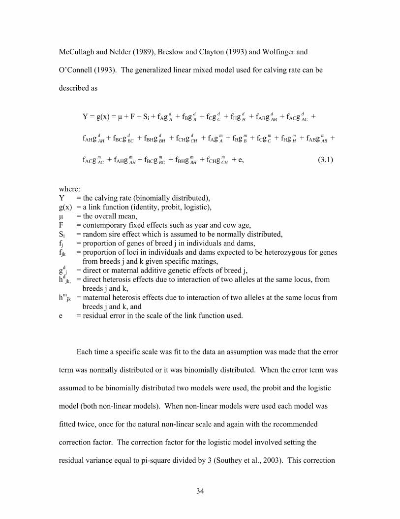
McCullagh and Nelder (1989), Breslow and Clayton (1993) and Wolfinger and

O’Connell (1993). The generalized linear mixed model used for calving rate can be

described as

Y = g(x) = µ + F + Si + fAg dA + fBg d

B + fCg dC + fHg d

H + fABg dAB + fACg d

AC +

fAHg dAH + fBCg d

BC + fBHg dBH + fCHg d

CH + fAg mA + fBg m

B + fCg mC + fHg m

H + fABg mAB +

fACg mAC + fAHg m

AH + fBCg mBC + fBHg m

BH + fCHg mCH + e, (3.1)

where: Y = the calving rate (binomially distributed), g(x) = a link function (identity, probit, logistic), µ = the overall mean, F = contemporary fixed effects such as year and cow age, Si = random sire effect which is assumed to be normally distributed, fj = proportion of genes of breed j in individuals and dams, fjk = proportion of loci in individuals and dams expected to be heterozygous for genes from breeds j and k given specific matings, gd

j = direct or maternal additive genetic effects of breed j, hd

jk, = direct heterosis effects due to interaction of two alleles at the same locus, from breeds j and k,

hmjk = maternal heterosis effects due to interaction of two alleles at the same locus from

breeds j and k, and e = residual error in the scale of the link function used.

Each time a specific scale was fit to the data an assumption was made that the error

term was normally distributed or it was binomially distributed. When the error term was

assumed to be binomially distributed two models were used, the probit and the logistic

model (both non-linear models). When non-linear models were used each model was

fitted twice, once for the natural non-linear scale and again with the recommended

correction factor. The correction factor for the logistic model involved setting the

residual variance equal to pi-square divided by 3 (Southey et al., 2003). This correction

35

factor assumes that the standard deviation of the logistic distribution equals to 1. This

could be an attempt to make the logistic distribution resemble the normal distribution

(thus making it more biologically interpretable). The correction factor used in the probit

model involved setting the residual variance equal to 1 (Heringstad et al., 2003).

In the first step, let ø = the vector of all unknown variance components (G, R) in

the generalized mixed model. G and R can be estimated if the mixed model matrix

system is solved iteratively to a convergence point. The GLIMMIX macro in SAS

estimates a (quasi) likelihood function L(ø) and the Fisher information matrix. During

the second step, the posterior distribution for ø given the data (y) was assumed to be

P(ø|y) = L(ø)*π(ø). The likelihood of the data given G and R is L(ø). The quasi-

likelihood of estimated function given ø was used for L(ø) (at convergence in

GLIMMIX) and π(ø) = prior knowledge (Fisher information matrix). The likelihood

information L(ø) and the prior information π(ø) are mixed to form the posterior

distribution P(ø|y). As the sample size of the data set increases the likelihood of the data

overwhelms the prior information.

Heritability Estimation

Estimation of variance components and subsequent heritability estimation was

conducted in a Bayesian frame work using the nonconjugate analysis of variance

(NBVC) methodology. In order to keep good frequentist behavior a Jeffrey prior was

used (Wolfinger and Kass, 2000). Using the GLIMMIX procedure the Bayesian

approach provides an easy to use alternative to restricted maximum likelihood estimation

(Wolfinger and Kass, 2000). Each time Model 3.1 was fit in the NBVC analysis the data

served as an initial prior for the independence sampling algorithm. The analysis is

36

performed with the PRIOR statement. The posterior analysis is performed after the

statistical algorithm (REML) used by the GLIMMIX macro converges. The default of

the sampling-based Bayesian analysis in SAS is to assume a Jeffreys’ prior and an

independence chain algorithm in order to generate the posterior sample (SAS, 2000).

After the final estimates of variance components and fixed effects are calculated, the

independence chain generates a pseudo-random proposal for the variance components

and fixed effects from a convenient base distribution. This distribution is chosen to be as

close as possible to the true posterior. This possible posterior function is determined

given all the observed data. Thus, the variance components proposed are conditioned on

all the observed data. The inverted gamma distribution is used as a posterior function. In

the first moment of the chain the initial value is the final estimates of GLIMMIX. New

values are proposed for fixed and random effects. GLIMMIX scores these new values

automatically as acceptable or not (acceptance rate) according to scores calculated from

the inverted gamma distribution. If the values are not acceptable a duplicate of the

previous values is entered into the chain and a new random value is proposed and scored.

If the second value was not accepted, the final estimates of random and fixed effects are

repeated and a new value is proposed as a third value. This process continues until the

sample size requested is achieved. In this research the sample size used was 10,000

pseudo-random samples of the variance components and fixed effects. Ten thousand was

used because the posterior mean of heritability is estimated with standard deviation

1/100th that of the parameter. This provides two decimal places of accuracy. The 10,000

values accepted by GLIMMIX are observations from the joint posterior distribution of

the sire and error variance as well as fixed effects (Wolfinger and Kass, 2000).

37

Heritability was estimated in the random sample of each posterior distribution and

stored in a separate data set. With the GLIMMIX macro 10,000 different estimates of the

posterior heritability were calculated for each statistical model for each trait of interest.

PROC KDE was used to approximate the final hypothesized probability mass function of

heritability. A posterior smooth function was computed for each mathematical model

with the kernel density estimation procedure of PROC KDE (SAS, 2000). The

descriptive statistics of this final distribution was calculated and graphed.

The graphs and descriptive statistics allow one to visualize the full impact of the

correction factors and the impact of the assumptions of a linear versus non-linear models.

Estimation of Breeding Value

Model 3.1 was fit to the data again without the continuous variables for direct and

maternal breed additive and nonadditive genetic effects to predict sire Expected Progeny

Differences (EPDs) for daughter calving rate and calf survival. The EPDs were predicted

with logistic, normal, and probit models. Spearman rank correlations between the EPDs

from different models were computed.

Predicted Performance for Crossbreeding Systems

Expected mean performance for CR and CS for straightbred and rotational breed

combinations were computed with ESTIMATE statements in the GLIMMIX macro (SAS,

2000). These mean performance values were computed using the estimated direct and

maternal breed additive and nonadditive genetic effects described in Model 3.

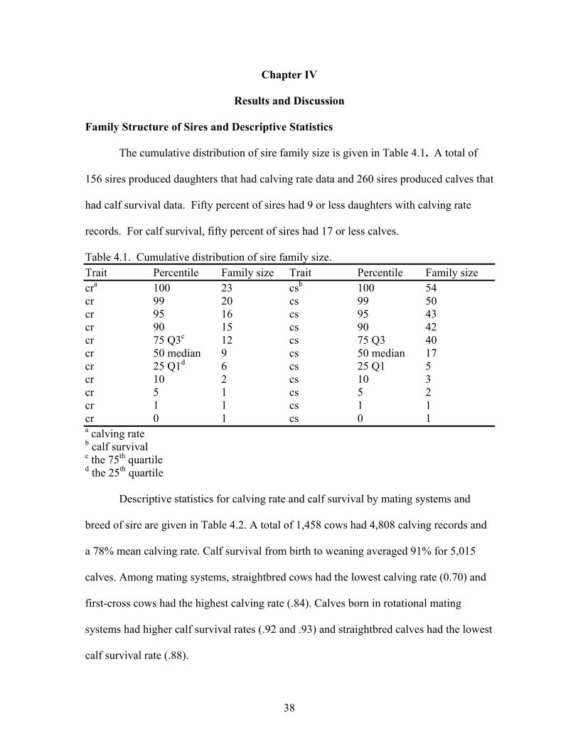
38

Chapter IV

Results and Discussion

Family Structure of Sires and Descriptive Statistics

The cumulative distribution of sire family size is given in Table 4.1. A total of

156 sires produced daughters that had calving rate data and 260 sires produced calves that

had calf survival data. Fifty percent of sires had 9 or less daughters with calving rate

records. For calf survival, fifty percent of sires had 17 or less calves.

Table 4.1. Cumulative distribution of sire family size. Trait Percentile Family size Trait Percentile Family size cra 100 23 csb 100 54 cr 99 20 cs 99 50 cr 95 16 cs 95 43 cr 90 15 cs 90 42 cr 75 Q3c 12 cs 75 Q3 40 cr 50 median 9 cs 50 median 17 cr 25 Q1d 6 cs 25 Q1 5 cr 10 2 cs 10 3 cr 5 1 cs 5 2 cr 1 1 cs 1 1 cr 0 1 cs 0 1 a calving rate b calf survival c the 75th quartile d the 25th quartile

Descriptive statistics for calving rate and calf survival by mating systems and

breed of sire are given in Table 4.2. A total of 1,458 cows had 4,808 calving records and

a 78% mean calving rate. Calf survival from birth to weaning averaged 91% for 5,015

calves. Among mating systems, straightbred cows had the lowest calving rate (0.70) and

first-cross cows had the highest calving rate (.84). Calves born in rotational mating

systems had higher calf survival rates (.92 and .93) and straightbred calves had the lowest

calf survival rate (.88).

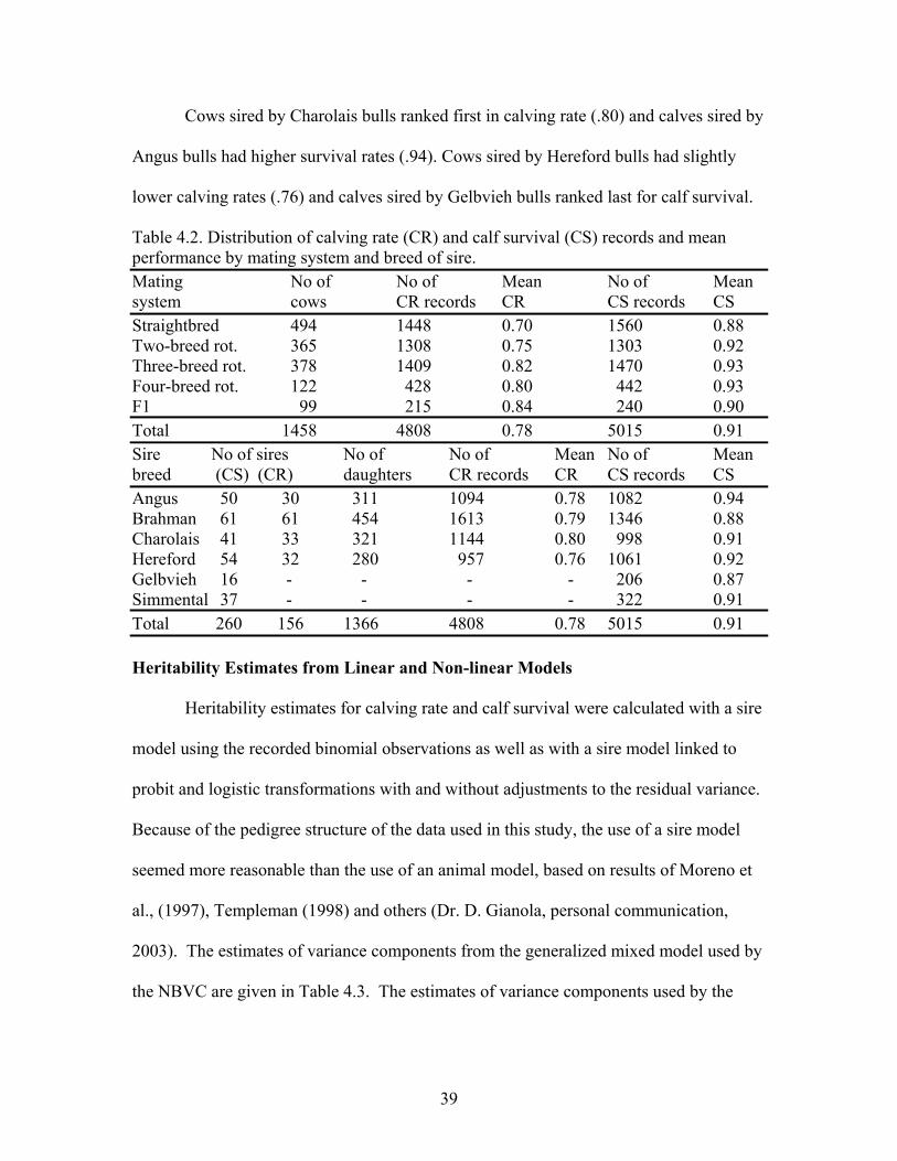
39

Cows sired by Charolais bulls ranked first in calving rate (.80) and calves sired by

Angus bulls had higher survival rates (.94). Cows sired by Hereford bulls had slightly

lower calving rates (.76) and calves sired by Gelbvieh bulls ranked last for calf survival.

Table 4.2. Distribution of calving rate (CR) and calf survival (CS) records and mean performance by mating system and breed of sire. Mating No of No of Mean No of Mean system cows CR records CR CS records CS Straightbred 494 1448 0.70 1560 0.88 Two-breed rot. 365 1308 0.75 1303 0.92 Three-breed rot. 378 1409 0.82 1470 0.93 Four-breed rot. 122 428 0.80 442 0.93 F1 99 215 0.84 240 0.90 Total 1458 4808 0.78 5015 0.91 Sire No of sires No of No of Mean No of Mean breed (CS) (CR) daughters CR records CR CS records CS Angus 50 30 311 1094 0.78 1082 0.94 Brahman 61 61 454 1613 0.79 1346 0.88 Charolais 41 33 321 1144 0.80 998 0.91 Hereford 54 32 280 957 0.76 1061 0.92 Gelbvieh 16 - - - - 206 0.87 Simmental 37 - - - - 322 0.91 Total 260 156 1366 4808 0.78 5015 0.91 Heritability Estimates from Linear and Non-linear Models

Heritability estimates for calving rate and calf survival were calculated with a sire

model using the recorded binomial observations as well as with a sire model linked to

probit and logistic transformations with and without adjustments to the residual variance.

Because of the pedigree structure of the data used in this study, the use of a sire model

seemed more reasonable than the use of an animal model, based on results of Moreno et

al., (1997), Templeman (1998) and others (Dr. D. Gianola, personal communication,

2003). The estimates of variance components from the generalized mixed model used by

the NBVC are given in Table 4.3. The estimates of variance components used by the

40

PROC KDE to compute the density of the posterior distribution of heritability are given

in Table 4.4.

Table 4.3. Quasi-likelihood estimates of sire component of variance (sirevar) and error variance (error). Model Model Model Model Model normal threshold(th) logistic(log) th/adjusted log/adjusted Calving rate Sirevar 0.0022* 0.0357* 0.0101* 0.0354* 0.1014*

Error 0.1547 0.9737 0.9710 1.0000 3.2865 Heritability 0.0560 0.1343 0.3782 0.1378 0.1197 Calf survival Sirevar 0.0006* 0.0320* 0.1235* 0.0320* 0.1235*

Error 0.0759 0.9739 0.9478 1.0000 3.2865 Heritability 0.0301 0.1312 0.4640 0.1240 0.1448 Heritability = 4*sirevar/(sirevar + error); *P<0.05. Table 4.4. Average of 10,000 estimates from the independence chain sampling of the posterior distribution of sire component of variance(sirevar) and error variance (error). Model Model Model Model Model normal threshold(th) logistic(log) th/adjusted log/adjusted Calving rate Sirevar 0.0024 0.0357 0.0106 0.0357 0.1068

Error 0.1548 0.9739 0.9711 1.0000 3.2865 Heritability 0.0610 0.1465 0.3962 0.1378 0.1197 Calf survival Sirevar 0.0007 0.0354 0.1360 0.0354 0.1360

Error 0.0760 0.9409 0.9349 1.0000 3.2865 Heritability 0.0365 0.1450 0.5079 0.1367 0.1589 Heritability = 4*sirevar/(sirevar + error); *P<0.05.

There is very little difference between the estimates in Table 4.3 and 4.4 which

indicates only a slight prior influence of the Fisher information matrix. The sire

component of variance was significantly different from zero in all statistical models. The

NBVC procedure of Wolfinger and Kass (2000) was needed to estimate the posterior

distribution of heritability for calving rate and calf survival for the logistic and logistic

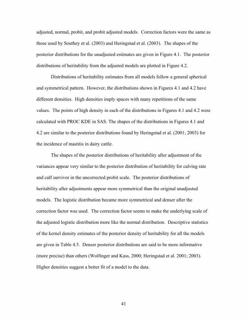
41

adjusted, normal, probit, and probit adjusted models. Correction factors were the same as

those used by Southey et al. (2003) and Heringstad et al. (2003). The shapes of the

posterior distributions for the unadjusted estimates are given in Figure 4.1. The posterior

distributions of heritability from the adjusted models are plotted in Figure 4.2.

Distributions of heritability estimates from all models follow a general spherical

and symmetrical pattern. However, the distributions shown in Figures 4.1 and 4.2 have

different densities. High densities imply spaces with many repetitions of the same

values. The points of high density in each of the distributions in Figures 4.1 and 4.2 were

calculated with PROC KDE in SAS. The shapes of the distributions in Figures 4.1 and

4.2 are similar to the posterior distributions found by Heringstad et al. (2001; 2003) for

the incidence of mastitis in dairy cattle.

The shapes of the posterior distributions of heritability after adjustment of the

variances appear very similar to the posterior distribution of heritability for calving rate

and calf survivor in the uncorrected probit scale. The posterior distributions of

heritability after adjustments appear more symmetrical than the original unadjusted

models. The logistic distribution became more symmetrical and denser after the

correction factor was used. The correction factor seems to make the underlying scale of

the adjusted logistic distribution more like the normal distribution. Descriptive statistics

of the kernel density estimates of the posterior density of heritability for all the models

are given in Table 4.5. Denser posterior distributions are said to be more informative

(more precise) than others (Wolfinger and Kass, 2000; Heringstad et al. 2001; 2003).

Higher densities suggest a better fit of a model to the data.

42

Densi t y

0

1

2

3

her i t abi l i t y

0. 0 0. 1 0. 2 0. 3 0. 4 0. 5 0. 6 0. 7 0. 8 0. 9 1. 0 1. 1

Densi t y

0. 0

0. 1

0. 2

0. 3

0. 4

0. 5

0. 6

0. 7

0. 8

0. 9

1. 0

1. 1

1. 2

1. 3

1. 4

1. 5

1. 6

1. 7

1. 8

1. 9

her i t abi l i t y

0. 0 0. 1 0. 2 0. 3 0. 4 0. 5 0. 6 0. 7 0. 8 0. 9 1. 0 1. 1 1. 2 1. 3

Densi t y

0

1

2

3

4

5

6

7

8

9

10

11

12

13

14

15

16

17

her i t abi l i t y

0. 00 0. 02 0. 04 0. 06 0. 08 0. 10 0. 12 0. 14 0. 16 0. 18 0. 20 0. 22 0. 24

Densi t y

0

1

2

3

4

5

6

7

8

9

10

11

12

13

14

15

16

17

18

19

20

her i t abi l i t y

0. 00 0. 01 0. 02 0. 03 0. 04 0. 05 0. 06 0. 07 0. 08 0. 09 0. 10 0. 11 0. 12 0. 13 0. 14

Densi t y

0

1

2

3

4

5

6

7

8

her i t abi l i t y

0. 00 0. 05 0. 10 0. 15 0. 20 0. 25 0. 30 0. 35 0. 40 0. 45

Densi t y

0

1

2

3

4

5

6

7

her i t abi l i t y

0. 00 0. 05 0. 10 0. 15 0. 20 0. 25 0. 30 0. 35 0. 40 0. 45 0. 50

Figure 4.1. Posterior density estimates of heritability. Calving rate estimates are to the left and calf survival estimates are to the right. From the top to the bottom the models represented are the logistic, normal, and probit.

CR, logistic CS, logistic

CR, normal CS, normal

CR, probit CS, probit

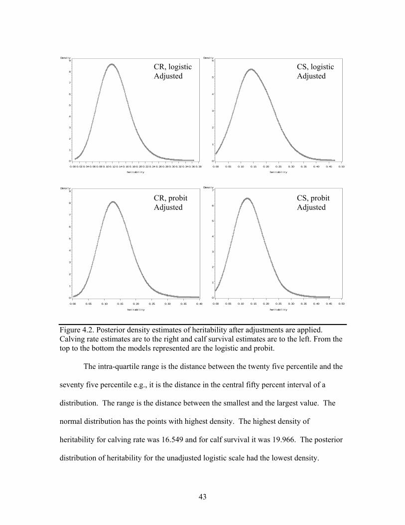
43

Densi t y

0

1

2

3

4

5

6

7

8

9

her i t abi l i t y

0. 00 0. 02 0. 04 0. 06 0. 08 0. 10 0. 12 0. 14 0. 16 0. 18 0. 20 0. 22 0. 24 0. 26 0. 28 0. 30 0. 32 0. 34 0. 36 0. 38

Densi t y

0

1

2

3

4

5

6

her i t abi l i t y

0. 00 0. 05 0. 10 0. 15 0. 20 0. 25 0. 30 0. 35 0. 40 0. 45 0. 50

Densi t y

0

1

2

3

4

5

6

7

8

9

her i t abi l i t y

0. 00 0. 05 0. 10 0. 15 0. 20 0. 25 0. 30 0. 35 0. 40

Densi t y

0

1

2

3

4

5

6

7

her i t abi l i t y

0. 00 0. 05 0. 10 0. 15 0. 20 0. 25 0. 30 0. 35 0. 40 0. 45 0. 50

Figure 4.2. Posterior density estimates of heritability after adjustments are applied. Calving rate estimates are to the right and calf survival estimates are to the left. From the top to the bottom the models represented are the logistic and probit.

The intra-quartile range is the distance between the twenty five percentile and the

seventy five percentile e.g., it is the distance in the central fifty percent interval of a

distribution. The range is the distance between the smallest and the largest value. The

normal distribution has the points with highest density. The highest density of

heritability for calving rate was 16.549 and for calf survival it was 19.966. The posterior

distribution of heritability for the unadjusted logistic scale had the lowest density.

CR, logisticAdjusted

CS, logisticAdjusted

CR, probit Adjusted

CS, probit Adjusted

44

Calving rate had the lowest intra-quartile range and range of the posterior distribution of

heritability under the normal model at 0.066 and 0.400. Calf survival had the lowest

intra-quartile and range of the posterior distribution of heritability under the normal

model at 0.085 and 0.490.

Heritability was estimated most precisely by the normal model and with least

precision by the unadjusted logistic model. The normal model was more precise because

its posterior distributions were denser than the posterior distributions from the other

models. The posterior distributions of the logistic and the threshold models for calf

survival were less dense than the other models.

The logistic model estimate of heritability, mode and confidence interval for

calving rate ( ± standard error) was 0.390 ± 0.130, 0.370, and 0.160 – 0.670, whereas the

corrected logistic model estimates of heritability, mode and confidence interval for

calving rate ( ± standard error) were 0.130 ± 0.045, 0.12, and 0.048 – 0.221. The logistic

model estimate of heritability, mode and confidence interval for calf survival (± standard

error) was 0.500 ± 0.200, 0.460, and 0.110 – 0.912, whereas the corrected logistic model

estimate of heritability, mode and confidence interval for calf survival ( ± standard error)

was 0.160 ± 0.070, 0.140, and 0.034 – 0.311, respectively.

The correction factor used in the logistic model improved the descriptive statistics

of the posterior distribution of heritability. The estimates of heritability from the probit

and adjusted probit models are similar to the estimates of heritability from the adjusted

logistic model. Agresti (2000) stated that the residual variance of the probit model is

naturally 1, unless severe over-dispersion or under-dispersion is present in the data. Thus

it appears that adjusting the residual variance of the probit model to 1 had minimal effect

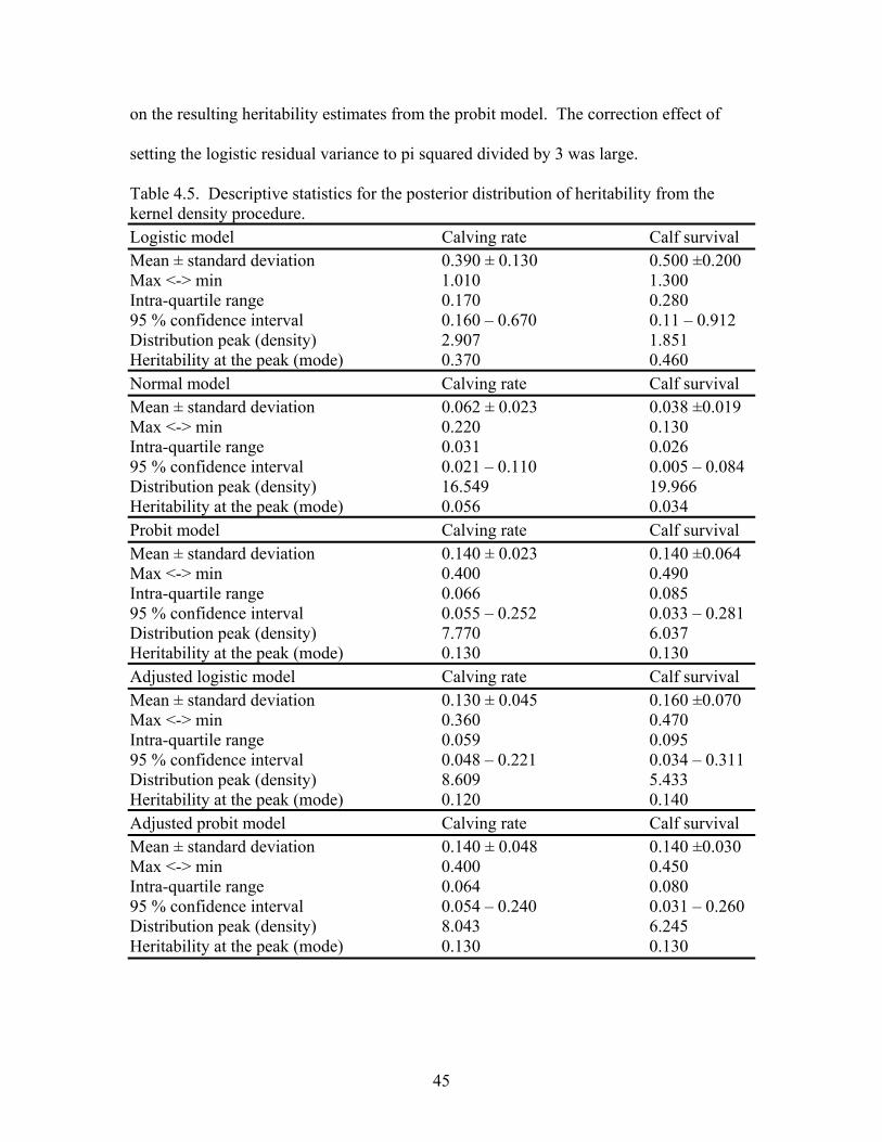
45

on the resulting heritability estimates from the probit model. The correction effect of

setting the logistic residual variance to pi squared divided by 3 was large.

Table 4.5. Descriptive statistics for the posterior distribution of heritability from the kernel density procedure. Logistic model Calving rate Calf survival Mean ± standard deviation 0.390 ± 0.130 0.500 ±0.200 Max <-> min 1.010 1.300 Intra-quartile range 0.170 0.280 95 % confidence interval 0.160 – 0.670 0.11 – 0.912 Distribution peak (density) 2.907 1.851 Heritability at the peak (mode) 0.370 0.460 Normal model Calving rate Calf survival Mean ± standard deviation 0.062 ± 0.023 0.038 ±0.019 Max <-> min 0.220 0.130 Intra-quartile range 0.031 0.026 95 % confidence interval 0.021 – 0.110 0.005 – 0.084 Distribution peak (density) 16.549 19.966 Heritability at the peak (mode) 0.056 0.034 Probit model Calving rate Calf survival Mean ± standard deviation 0.140 ± 0.023 0.140 ±0.064 Max <-> min 0.400 0.490 Intra-quartile range 0.066 0.085 95 % confidence interval 0.055 – 0.252 0.033 – 0.281 Distribution peak (density) 7.770 6.037 Heritability at the peak (mode) 0.130 0.130 Adjusted logistic model Calving rate Calf survival Mean ± standard deviation 0.130 ± 0.045 0.160 ±0.070 Max <-> min 0.360 0.470 Intra-quartile range 0.059 0.095 95 % confidence interval 0.048 – 0.221 0.034 – 0.311 Distribution peak (density) 8.609 5.433 Heritability at the peak (mode) 0.120 0.140 Adjusted probit model Calving rate Calf survival Mean ± standard deviation 0.140 ± 0.048 0.140 ±0.030 Max <-> min 0.400 0.450 Intra-quartile range 0.064 0.080 95 % confidence interval 0.054 – 0.240 0.031 – 0.260 Distribution peak (density) 8.043 6.245 Heritability at the peak (mode) 0.130 0.130

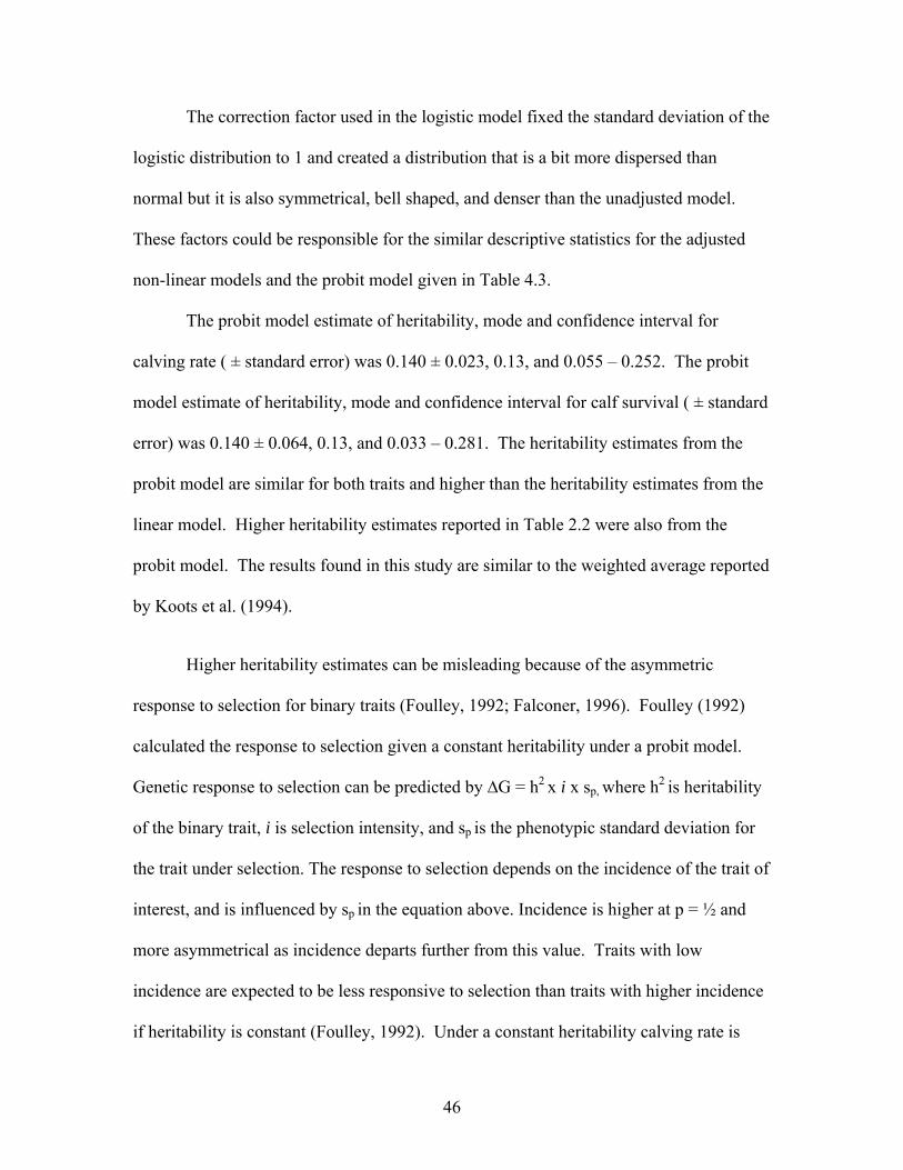
46

The correction factor used in the logistic model fixed the standard deviation of the

logistic distribution to 1 and created a distribution that is a bit more dispersed than

normal but it is also symmetrical, bell shaped, and denser than the unadjusted model.

These factors could be responsible for the similar descriptive statistics for the adjusted

non-linear models and the probit model given in Table 4.3.

The probit model estimate of heritability, mode and confidence interval for

calving rate ( ± standard error) was 0.140 ± 0.023, 0.13, and 0.055 – 0.252. The probit

model estimate of heritability, mode and confidence interval for calf survival ( ± standard

error) was 0.140 ± 0.064, 0.13, and 0.033 – 0.281. The heritability estimates from the

probit model are similar for both traits and higher than the heritability estimates from the

linear model. Higher heritability estimates reported in Table 2.2 were also from the

probit model. The results found in this study are similar to the weighted average reported

by Koots et al. (1994).

Higher heritability estimates can be misleading because of the asymmetric

response to selection for binary traits (Foulley, 1992; Falconer, 1996). Foulley (1992)

calculated the response to selection given a constant heritability under a probit model.

Genetic response to selection can be predicted by ∆G = h2 x i x sp, where h2 is heritability

of the binary trait, i is selection intensity, and sp is the phenotypic standard deviation for

the trait under selection. The response to selection depends on the incidence of the trait of

interest, and is influenced by sp in the equation above. Incidence is higher at p = ½ and

more asymmetrical as incidence departs further from this value. Traits with low

incidence are expected to be less responsive to selection than traits with higher incidence

if heritability is constant (Foulley, 1992). Under a constant heritability calving rate is

47

expected to be more responsive to selection than calf survival because a cow failing to

calf is more frequent than a calf failing to survive to weaning age. It is more reasonable

to be more conservative and more precise with the linear model estimates since response

to selection will be realized in the observed scale.

The normal model estimate of heritability, mode and confidence interval for

calving rate ( ± standard error) was 0.062 ± 0.023, 0.056, and 0.021 – 0.110 and the

normal model estimate of heritability, mode and confidence interval for calf survival ( ±

standard error) was 0.038 ± 0.019, 0.034, and 0.005 – 0.084.

Deviances and scaled deviances of each of the models were computed and are

recorded in Table 4.6. The deviance is a likelihood ratio test for the fit of each model to

the data compared to a complete model. The logistic and the probit models failed to fit

the data for calf survival, but did fit the data for calving rate. When ө is substantially

different from one, the likelihood ratio test was based on the scaled-deviance. The

scaled-deviance is the deviance divided by ө (Littlell, et al., 1996).

Table 4.6. The deviance and scaled deviance of the models used to analyze calving rate (cr) and calf survival (cs). Models (model 3.1) ө Deviance Scaled Deviance df A: normal (cr) 0.1533 720.9173** 4701.9828 3728

B: probit (cr) 0.9868 4466.8618 4526.6271 3728 C: logistic (cr) 0.9710 4534.6673 4670.2364 3728 D: normal (cs) 0.0730 348.0823** 4770.0302 4790 E: probit (cs) 1.1722 2704.6380** 2136.7096** 4790 F: logistic (cs) 1.0619 2705.4990** 2327.4911** 4790

Using the scaled deviance (because ө was different from 1), the normal model fit

both the CR and CS data. Based on the density of sampled heritability estimates with the

normal model for both CR and CS, and the fit of the scaled deviance of the normal model

48

for both traits, heritability estimates from the normal model appear to be more reasonable

and applicable than the heritability estimates from the other models.

Comparison and Description of Expected Progeny Differences

Sire EPDs for daughter calving rate and for calf survival are given in appendix A

and B in the normal scale because it is assumed to be more precise with these data. The

cumulative distributions of EPDs for calving rate from the logistic, normal and probit

models are shown in Tables 4.7, 4.8 and 4.9. These distributions clearly show that EPDs

from the logistic model have a greater range than other models. In fact, the range of EPDs

from the logistic model for calving rate (-.38 to +.48) and calf survival (-.76 to +.77) are

biologically unrealistic. EPDs were calculated to compare sires for possible selection in a

breeding program. A sire with an EPD of .77 for calf survival would be expected to sire

progeny that had a 153 % greater survival rate than a sire with an EPD for progeny

survival rate of -.76. This result is not reasonable nor is it biologically possible. Since

EPDs are estimated as deviations from the mean, an EPD of +.77 for calf survival is not

reasonable for a calf survival mean of 91 percent. Even the transformed scales resulted in

slightly out of range EPDs for reasonable interpretation.

The values given in Table 4.7 are expressed in the logistic scale or the lod-score

scale. None of these scores is higher than 3 or smaller than -2, indicating that sire EPDs

are not closely associated with calving rate and calf survival, based on the interpretation

given by Weir (1996). This is not unexpected as heritability estimates were relatively

low, meaning that the environmental portion of phenotypic variance accounts for a much

larger proportion of the phenotypic variance than genetic variance.

49

The distribution of sire EPDs in Table 4.8 obtained from the normal model

appears more biologically acceptable in that the ranges are more realistic. A sire with an

EPD for calving rate of 0.09 is expected to sire daughters with a 15% higher probability

of calving than a sire with an EPD of -0.06.

The cumulative distribution of sire breeding values from the probit model is given

in Table 4.9. Values in Table 4.9 are expressed as z-scores. The z-scores can only be

interpreted if the z-transformation is applied to them. After transforming sire EPDs from

the logistic scale (elod-score/1+elod-score) and probit scale (converting the EPDs from the

probit model with a table with z-scores) and after subtracting the mean from each value

in each of the scales, adjusted sire EPDs are given in Tables 4.10 and 4.11. The

magnitude of differences between the EPDs in Tables 4.10 and 4.11 is largely

unimportant. More computations were necessary with non-linear models to obtain results

similar to those obtained with a regular linear model. With large data sets such as those

from breed associations, the linear model should be considered more practical (Pochas

and Laloe, 2003).

Table 4.7. Cumulative distribution of sire breeding values for calving rate and calf survival estimated with the logistic model. trait percentile EPD trait percentile EPD cr 100 0.46 cs 100 0.77 cr 99 0.44 cs 99 0.67 cr 95 0.29 cs 95 0.50 cr 90 0.22 cs 90 0.38 cr 75 Q3 0.10 cs 75 Q3 0.16 cr 50 median 0.01 cs 50 median 0.04 cr 25 Q1 -0.11 cs 25 Q1 -0.20 cr 10 -0.23 cs 10 -0.40 cr 5 -0.31 cs 5 -0.54 cr 1 -0.38 cs 1 -0.76

50

Table 4.8. Cumulative distribution of sire breeding values for calving rate and calf survival estimated with the normal model. trait percentile EPD trait percentile EPD cr 100 0.06 cs 100 0.03 cr 99 0.05 cs 99 0.03 cr 95 0.03 cs 95 0.02 cr 90 0.03 cs 90 0.01 cr 75 Q3 0.01 cs 75 Q3 0.00 cr 50 median 0.00 cs 50 median 0.00 cr 25 Q1 -0.01 cs 25 Q1 -0.00 cr 10 -0.03 cs 10 -0.01 cr 5 -0.04 cs 5 -0.02 cr 1 -0.05 cs 1 -0.04 Table 4.9. Cumulative distribution of sire breeding values for calving rate and calf survival estimated with the probit model. trait percentile EPD trait percentile EPD cr 100 0.26 cs 100 0.33 cr 99 0.26 cs 99 0.31 cr 95 0.17 cs 95 0.21 cr 90 0.12 cs 90 0.17 cr 75 Q3 0.05 cs 75 Q3 0.07 cr 50 median 0.00 cs 50 median 0.02 cr 25 Q1 -0.06 cs 25 Q1 -0.08 cr 10 -0.13 cs 10 -0.18 cr 5 -0.17 cs 5 -0.23 cr 1 -0.22 cs 1 -0.34 progeny differences for calving rate estimated by the transformed non-linear models are

Table 4.10. Cumulative distribution of sire breeding values for calving rate and calf survival estimated with the transformed logistic model. trait percentile EPD trait percentile EPD cr 100 0.10 cs 100 0.18 cr 99 0.10 cs 99 0.16 cr 95 0.06 cs 95 0.12 cr 90 0.04 cs 90 0.09 cr 75 Q3 0.02 cs 75 Q3 0.04 cr 50 median 0.00 cs 50 median 0.01 cr 25 Q1 -0.02 cs 25 Q1 -0.05 cr 10 -0.05 cs 10 -0.10 cr 5 -0.06 cs 5 -0.13 cr 1 -0.08 cs 1 -0.18

51

Table 4.11. Cumulative distribution of sire breeding values for calving rate and calf survival estimated with the transformed probit model. trait percentile EPD trait percentile EPD cr 100 0.11 cs 100 0.13 cr 99 0.10 cs 99 0.12 cr 95 0.07 cs 95 0.08 cr 90 0.05 cs 90 0.06 cr 75 Q3 0.02 cs 75 Q3 0.02 cr 50 median 0.00 cs 50 median 0.00 cr 25 Q1 -0.02 cs 25 Q1 -0.03 cr 10 -0.05 cs 10 -0.07 cr 5 -0.07 cs 5 -0.09 cr 1 -0.09 cs 1 -0.14

Spearman correlations are given in Tables 4.12 and 4.13. These correlations

detect the degree of dissimilar rankings. All correlations were .98 or above. Weller et al.

(1988) found correlations of .98 or above between breeding values predicted by linear

and threshold models for calf mortality. Heringstad et al. (2003) also found correlations

of .99 between breeding values predicted by linear and threshold models for calving ease.

Table 4.12. Spearman rank correlations between sire EPD values for calving rate from all models. nepd lepd pepd tlepd tpepd

Linear EPDs (nepd) 1.00 0.99 0.99 0.99 0.99 Logistic EPDs (lepd) 0.99 1.00 0.99 0.99 0.99 Probit EPDs (pepd) 0.99 0.99 1.00 0.99 0.99 Transformed logistic (tlepd) 0.99 0.99 0.99 1.00 0.99 Transformed probit (tpepd) 0.99 0.99 0.99 0.99 1.00

Table 4.13. Spearman rank correlations between sire EPD values for calf survival from all models. nepd lepd pepd tlepd tpepd

Linear EPDs (nepd) 1.00 0.98 0.98 0.98 0.98 Logistic EPDs (lepd) 0.98 1.00 0.99 0.99 0.99 Probit EPDs (pepd) 0.98 0.99 1.00 0.99 0.99 Transformed logistic (tlepd) 0.98 0.99 0.99 1.00 0.99 Transformed probit (tpepd) 0.98 0.99 0.99 0.99 1.00

Very high positive correlations were observed between EPDs from all models.

This means that the transformations used with the logistic and probit models resulted in

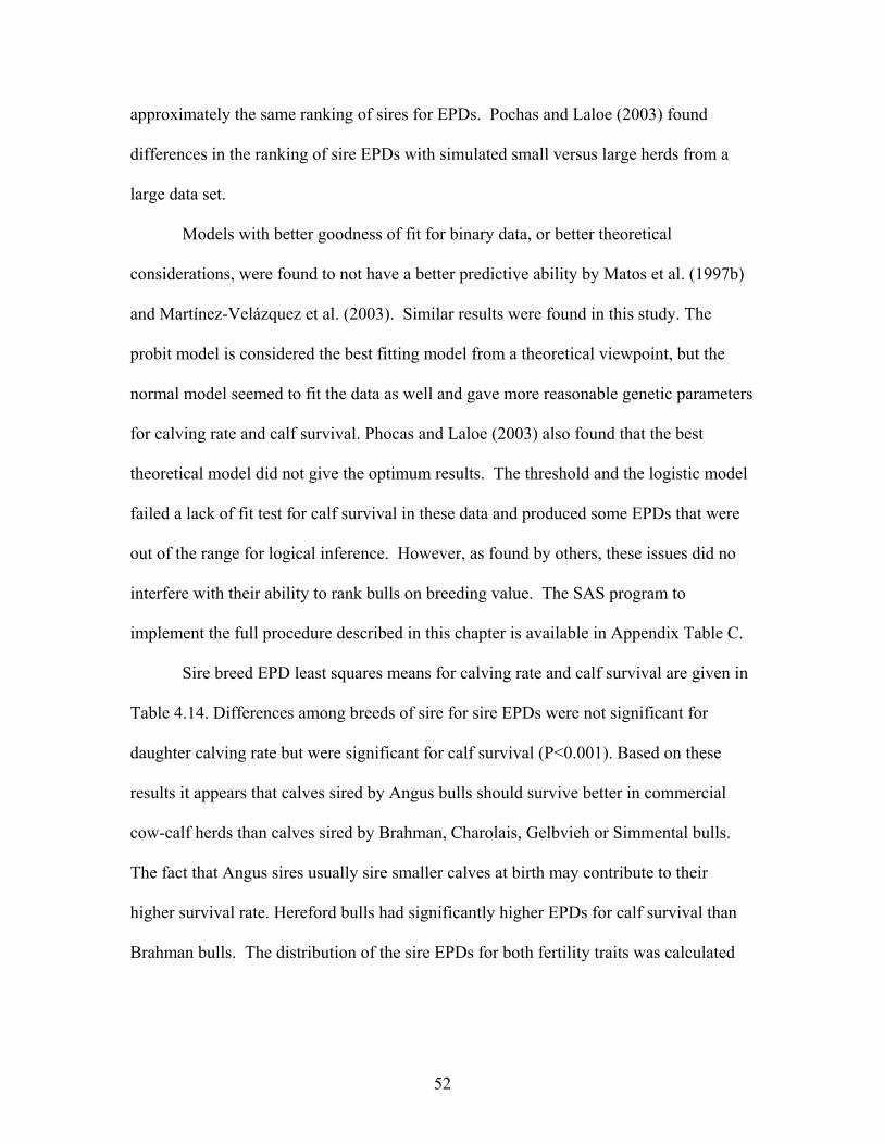
52

approximately the same ranking of sires for EPDs. Pochas and Laloe (2003) found

differences in the ranking of sire EPDs with simulated small versus large herds from a

large data set.

Models with better goodness of fit for binary data, or better theoretical

considerations, were found to not have a better predictive ability by Matos et al. (1997b)

and Martínez-Velázquez et al. (2003). Similar results were found in this study. The

probit model is considered the best fitting model from a theoretical viewpoint, but the

normal model seemed to fit the data as well and gave more reasonable genetic parameters

for calving rate and calf survival. Phocas and Laloe (2003) also found that the best

theoretical model did not give the optimum results. The threshold and the logistic model

failed a lack of fit test for calf survival in these data and produced some EPDs that were

out of the range for logical inference. However, as found by others, these issues did no

interfere with their ability to rank bulls on breeding value. The SAS program to

implement the full procedure described in this chapter is available in Appendix Table C.

Sire breed EPD least squares means for calving rate and calf survival are given in

Table 4.14. Differences among breeds of sire for sire EPDs were not significant for

daughter calving rate but were significant for calf survival (P<0.001). Based on these

results it appears that calves sired by Angus bulls should survive better in commercial

cow-calf herds than calves sired by Brahman, Charolais, Gelbvieh or Simmental bulls.

The fact that Angus sires usually sire smaller calves at birth may contribute to their

higher survival rate. Hereford bulls had significantly higher EPDs for calf survival than

Brahman bulls. The distribution of the sire EPDs for both fertility traits was calculated

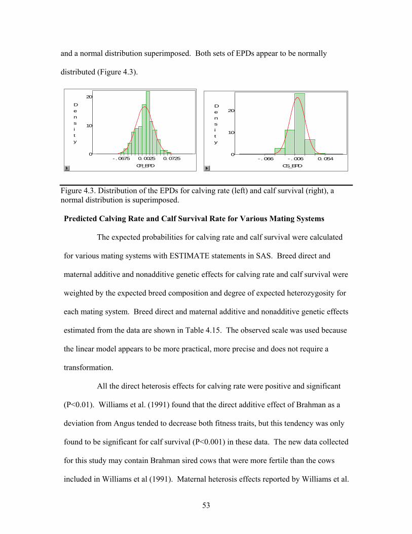
53

and a normal distribution superimposed. Both sets of EPDs appear to be normally

distributed (Figure 4.3).

- . 0675 0. 0025 0. 0725

CR_EPD

0

10

20

Density

- . 066 - . 006 0. 054

CS_EPD

0

10

20Density

Figure 4.3. Distribution of the EPDs for calving rate (left) and calf survival (right), a normal distribution is superimposed. Predicted Calving Rate and Calf Survival Rate for Various Mating Systems The expected probabilities for calving rate and calf survival were calculated

for various mating systems with ESTIMATE statements in SAS. Breed direct and

maternal additive and nonadditive genetic effects for calving rate and calf survival were

weighted by the expected breed composition and degree of expected heterozygosity for

each mating system. Breed direct and maternal additive and nonadditive genetic effects

estimated from the data are shown in Table 4.15. The observed scale was used because

the linear model appears to be more practical, more precise and does not require a

transformation.

All the direct heterosis effects for calving rate were positive and significant

(P<0.01). Williams et al. (1991) found that the direct additive effect of Brahman as a

deviation from Angus tended to decrease both fitness traits, but this tendency was only

found to be significant for calf survival (P<0.001) in these data. The new data collected

for this study may contain Brahman sired cows that were more fertile than the cows

included in Williams et al (1991). Maternal heterosis effects reported by Williams et al.

54

(1991) are equivalent to direct heterosis effects in this study. The only effects that

influenced calf survival positively and significantly were the maternal heterosis effects

of A-B and B-H (P<0.01). The direct A-B heterosis effect had the largest influence

(0.2452 ± 0.0387; P<0.01) on calving rate and the A-B maternal heterosis effect had the

largest effect on calf survival (0.0842 ± 0.0268; P<0.01). These results are consistent

with those of Comerford et al. (1987), and highlight the importance of the Brahman

breed in the Gulf Coast Region.

Predicted probabilities for calving rate and calf survival for various mating

systems are given in Table 4.16. The poorest mating system for calving rate and calf

survival was the straightbred Brahman (0.57 ± 0.02 and 0.81 ± 0.01, respectively). The

lower calving rate and calf survival of Brahman has been observed by others (Turner et

al., 1968; Cundiff, 1970; Long, 1980; Williams et al., 1990). The best mating system for

calving rate was the A-H two-breed rotation system (0.93 ± 0.07), and the best system

for calf survival was the A-B-H three-breed rotation system (0.98 ± 0.03). The A-B-H

rotation system had a high probability for calving rate (0.88 ± 0.03) and the highest

probability for calf survival, making it one of the better mating systems in these data.

The H-B two-breed rotation cows had a higher calving rate than A-B or C-B

two-breed rotation cows as was reported by Williams et al. (1991). Three- and four-

breed rotation systems had slightly lower predicted calving rate than two-bred rotation

systems, however two-breed rotation systems had slightly lower calf survival rates than

three- and four-breed rotation systems. Williams et al. (1991) reported non-significant

differences among two-, three- and four-breed rotation systems for calving rate.

Crossbreds derived from various breed combinations that do not include

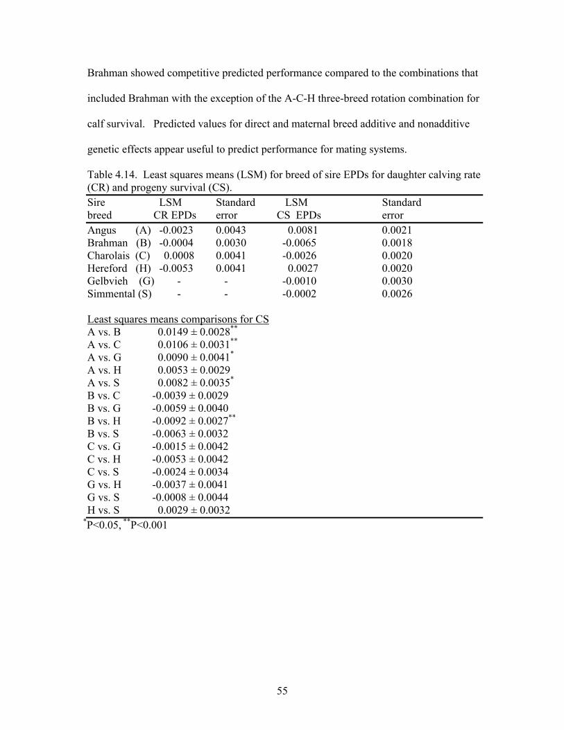
55

Brahman showed competitive predicted performance compared to the combinations that

included Brahman with the exception of the A-C-H three-breed rotation combination for

calf survival. Predicted values for direct and maternal breed additive and nonadditive

genetic effects appear useful to predict performance for mating systems.

Table 4.14. Least squares means (LSM) for breed of sire EPDs for daughter calving rate (CR) and progeny survival (CS). Sire LSM Standard LSM Standard breed CR EPDs error CS EPDs error Angus (A) -0.0023 0.0043 0.0081 0.0021 Brahman (B) -0.0004 0.0030 -0.0065 0.0018 Charolais (C) 0.0008 0.0041 -0.0026 0.0020 Hereford (H) -0.0053 0.0041 0.0027 0.0020 Gelbvieh (G) - - -0.0010 0.0030 Simmental (S) - - -0.0002 0.0026 Least squares means comparisons for CS A vs. B 0.0149 ± 0.0028**

A vs. C 0.0106 ± 0.0031** A vs. G 0.0090 ± 0.0041* A vs. H 0.0053 ± 0.0029 A vs. S 0.0082 ± 0.0035* B vs. C -0.0039 ± 0.0029 B vs. G -0.0059 ± 0.0040 B vs. H -0.0092 ± 0.0027** B vs. S -0.0063 ± 0.0032 C vs. G -0.0015 ± 0.0042 C vs. H -0.0053 ± 0.0042 C vs. S -0.0024 ± 0.0034 G vs. H -0.0037 ± 0.0041 G vs. S -0.0008 ± 0.0044 H vs. S 0.0029 ± 0.0032

*P<0.05, **P<0.001

56

Table 4.15. Direct and maternal breed additive and nonadditive genetic effects for calving rate and calf survival.

Breed Calving Calf sourcea rate ± SD survival ± SD Direct effects Brahman (B) -0.0767 ± 0.0579 -0.1279 ± 0.0337**

Charolais (C) 0.0430 ± 0.0590 -0.0429 ± 0.0459 Hereford (H) -0.0080 ± 0.0591 -0.0339 ± 0.0334 Gelbvieh (G) - -0.1450 ± 0.0640**

Simmental (S) - -0.0893 ± 0.0650 Direct heterosis effects AB 0.2452 ± 0.0387** 0.0123 ± 0.0264 AC 0.1660 ± 0.0671** -0.0801 ± 0.0833 AH 0.2104 ± 0.0607** -0.0041 ± 0.0382 BC 0.1787 ± 0.0413** 0.0116 ± 0.0334 BH 0.1995 ± 0.0399** 0.0044 ± 0.0302 CH 0.1663 ± 0.0646** 0.0574 ± 0.0791 Maternal effects Brahman (B) -0.0406 ± 0.0516 -0.0230 ± 0.0311 Charolais (C) -0.0168 ± 0.0537 0.0114 ± 0.0480 Hereford (H) 0.0334 ± 0.0564 0.0020 ± 0.0348 Maternal heterosis effects AB -0.0580 ± 0.0368 0.0842 ± 0.0268** AC -0.0565 ± 0.0728 -0.0227 ± 0.0672 AH -0.0707 ± 0.0663 0.0020 ± 0.0325 BC -0.0234 ± 0.0392 0.0839 ± 0.0497 BH -0.0146 ± 0.0406 0.0151 ± 0.0297** CH -0.0186 ± 0.0652 -0.0174 ± 0.0714 aBreed direct and maternal genetic effects expressed as deviation from Angus. *P < 0.05, **P < 0.01. It is more complex to manage three-breed and four-breed rotational systems than

two-breed rotational systems. The differences between rotational crossbreeding systems

appear to be small. The differences between two-, three-, and four-breed rotational

systems and the straightbred systems are larger for calving rate than for calf survival. In

order to improve fertility, commercial herds could use a two-breed rotational system or

purchase replacement females that are crossbred. The standard errors of the predictions

57

for the two-, three-, and four-breed rotational systems are larger than the standard errors

of the straightbreds.

Table 4.16. Predicted calving rate and calf survival for major mating systems Mating Predicted Predicted system CR ± Std. Err. CS ± Std. Err Straightbred Angus (A) 0.69 ± 0.02 0.91 ± 0.01 Brahman (B) 0.57 ± 0.02 0.81 ± 0.01 Charolais (C) 0.71 ± 0.02 0.88 ± 0.01 Hereford (H) 0.71 ± 0.02 0.88 ± 0.01 Two-breed rotation combinations A-B 0.85 ± 0.04 0.86 ± 0.03 A-C 0.86 ± 0.07 0.82 ± 0.09 A-H 0.93 ± 0.07 0.89 ± 0.04 B-C 0.83 ± 0.04 0.88 ± 0.04 B-H 0.88 ± 0.04 0.87 ± 0.02 C-H 0.90 ±0.07 0.93 ± 0.08 Three-breed rotation combinations A-B-C 0.83 ± 0.04 0.92 ± 0.07 A-B-H 0.88 ± 0.03 0.98 ± 0.03 B-C-H 0.84 ± 0.04 0.89 ± 0.05 A-C-H 0.87 ± 0.07 0.84 ± 0.06 Four-breed rotation combination A-B-C-H 0.81 ± 0.03 0.91 ± 0.01

58

Chapter V

Summary and Implications

Genetic evaluation for calving rate and calf survival was conducted with

linear and non-linear statistical models. The linear (normal) model was more precise and

required fewer manipulations (transformations) than non-linear models. Computer

software for linear models is easier to obtain and to manipulate than software for non-

linear models. In SAS, a macro was used in order to fit non-linear models. A linear

model appeared to be more practical and produced heritability estimates that were more

applicable to industry. The normal linear model appeared optimum for predicting

biologically sound EPDs for calving rate and calf survival.

The EPDs for both traits appears to be normally distributed as expected. Not

calculating EPDs for economically relevant fertility traits means that direct improvement

for the trait is not being achieved. Both traits were lowly heritable but the sire

component of variance was statistically different from zero. Slow but positive genetic

improvement in calving rate and calf survival could be made.

Two breed rotational combinations had higher predicted calving rate

performance than three- or four-breed rotation combinations. Three-breed rotational

combinations tended to have a higher predicted performance for calf survival. Calculation

of direct and maternal breed additive and nonadditive genetic effects for all breeds in

Louisiana could lead to predicted performance of breeds and combinations not evaluated

as purebreds or as crossbreds. Thus, identification of the better breeds and breed

combinations could be identified for this environment.

59

References

Abdel-Azim, G. A. and P. J. Berger. 1999. Properties of threshold model predictions. J. Anim. Sci. 77:582. Agresti, A. 2002. Categorical Data Analysis. John Wiley & Sons, Inc. New York. Anderson, L., and M. Georges. 2004. Domestic-animal genomics: deciphering the genetics of complex traits. Nature 5:202. Bernardo, J. M., and A. F. M. Smith. 2002. Bayesian Theory. John Wiley & Sons, New

York. Black, W. H., and, J. L. Lush. 1934. Beef production and quality as influenced by crossing Brahman with Hereford and Shorthorn cattle. U.S. Dept. Agr. Tech. Bull. 417. Breslow, N. R. and D. G. Clayton. 1993. Approximate inference in generalized linear mixed models. J. Amer. Stat. Assoc. 88:9. Cartwright, T. C., G. F. Ellis, Jr., W. E. Kruse, and E. K. Croch. 1964. Hybrid vigor in Brahman-Hereford crosses. Texas Agric. Exp. Sta. Tech. Monogr. 1, College Station. Comerford, J. S., J. K. Bertrand, L. L. Benyshek, and M. H. Johnson. 1987. Reproductive rates, birth weight, calving ease and 24-H calf survival in a four- breed rotational system among Simmental, Limousin, Polled Hereford and Brahman beef cattle. J. Anim Sci. 64:65. Cundiff, L. V. 1970. Selection criteria for beef cattle of the future. J. Anim. Sci. 30:694. Cundiff, L. V., K. E. Gregory, and R. M. Koch. 1974. Effects of heterosis on reproduction in Hereford, Angus, and Shorthorn cattle. J. Anim. Sci. 38:711. Curnow, R. N., and C. Smith. 1975. Multifactorial models for familial diseases in man. J. Roy. Statist. Soc. A. 138:375. Dempster, E. R., and I. M. Lerner. 1950. Heritability of threshold characters. Genetics 35:212. Devore, J. L. 2000. Probability and Statistics for Engineering and the Sciences. ITP Publishing, Inc. California. Dickerson, G. E. 1970. Efficiency of animal production-modeling the biological components. J. Anim. Sci. 30:1032.

60

Dickerson, G. E. 1973. Inbreeding and heterosis in animals. IN: Proc. Amer. Breed. and Genet. Symposium in honor of J. L. Lush, p. 54, ASA, ADSA and PSA. Champaign, IL. Donoghue, K. A., R. Rekaya, J. K. Bertrand, and I. Misztal. 2004. Threshold-linear analysis of measures of fertility in artificial insemination data and days to calving in beef cattle. J. Anim. Sci. 82:987. Doyle, S. P., R. D. Green, B. L. Golden, G. L. Mathiews, C. R. Comstocks, and D. G. LeFever. 1996. Genetic parameter estimates for pregnancy rate and subsequent rebreeding rate in Angus cattle. J. Anim. Sci. 74 (Suppl.1):117 (Abstr.). Doyle, S. P., B. L. Golden, R. D. Green, and J. S. Brinks. 2000. Additive

geneticparameter estimates for heifer pregnancy and subsequent reproductive performance in Angus females. J. Anim. Sci. 78:2091.

Eler, J. P., J. A. II V. Silva, J. B. S. Ferraz, F. Dias, H. N. Oliveira, J. L. Evans, and B. L. Golden. 2002. Genetic evaluation of the probability of pregnancy at 14 months for Nellore heifers. J. Anim. Sci. 80:951. Eisen, E. J., G. Horstgen-Scwark, A. M. Saxton, and T. R. Bandy. 1983. Genetic interpretation and analysis of diallel crosses with animals. Theor. Appl. Genet. 65:17. Evans, J. L. B. L. Golden, R. M. Bourdon, and K. L. Long. 1999. Additive genetic relationship between heifer pregnancy and scrotal circumference in Hereford cattle. J. Anim. Sci. 77:2621. Falconer, D. S. 1965. The inheritance of liability to certain diseases estimated from the incidence among relatives. Ann. Human Genetics. 29:51. Falconer, D. S. 1989. Introduction to Quantitative Genetics. Longman, Londom. Foulley, J. L. 1992. Prediction of selection response for threshold dichotomous traits. Genetics 132:1187. Franke. D. E. 1980. Breed and heterosis effects of American Zebu Cattle. J. Anim. Sci. 48:83. Franke, D. E., O. Habet, L. C. Tawah, A. R. Williams, and S. M. DeRouen. 2001. Direct and maternal genetic effects on birth and weaning traits in multibreed cattle and predicted performance of breed crosses. J. Anim. Sci. 79:1713.

61

Gaines, J. A., W. H. McClure, D. W. Vogot, R. C. Carter, and C. M. Kincaid. 1966. Heterosis from crosses among British breeds of beef cattle: Fertility and calf performance to weaning. J. Anim. Sci. 25:5. Gianola. D. 1982. Theory and analysis of threshold characters. J. Anim. Sci. 54:1079. Gianola D., and R. L. Fernando. 1986. Bayesian methods in animal breeding theory. J. Anim. Sci. 63:217. Gianola, D., and J. L. Foulley. 1983. Sire evaluation for ordered categorical data with a threshold model. Genet. Sel. Evol. 15:201. Gianola, D., and J. L. Foulley. 1996. Statistical analysis of ordered categorical data via a structured heteroskedastic threshold model. Genet. Sel. Evol. 28:249. Gregory, K. E., L. V. Cundiff, and R. M. Koch. 1991. Breed effects and heterosis in advanced generations of composite populations on actual weight, adjusted weight, hip height, and condition scores of beef cows. J. Anim. Sci. 73:1742. Hagger, C., and A. Hofer. 1989. Correlations between breeding values of dairy dairy sires for frequency of dystocia evaluated by a linear and non linear method. J. Anim. Sci. 67(suppl.1)(Abstr.). Harville, D. A. 1976. Extension of the Gauss-Markov theorem to include the estimation

of random effects. Ann. of Stat. 2:384. Harville, D. A. 1977. Maximum likelihood approach to variance component estimation and to related problems. J. Am. Stat. Assoc. 72:320. Hayes, B., R. K. Shepherd, and S. Newman. 2002. Look ahead mate selection schemes for multi-breed beef populations. Anim. Sci. 74:13. Henderson, C. R. 1952. Specific and General Combining Ability. IN: John W. Gowen (ed.) Heterosis. Iowa State College Press, Ames, Iowa. Henderson, C. R. 1976. A simple method for computing the inverse of a numerator relationship matrix used in predicting of breeding values. Biometrics 32: 69. Henderson, C. R. 1984. Application of Linear Models in Animal Breeding. University of

Guelph, Canada. Heringstad, B., D. Gianola, G. Klemetsdal, and K. A. Weigel. 2001. Bayesian analysis of liability of clinical mastitis in Norwegian cattle with a threshold model: effects of data sampling method. J. Dairy Sci. 84:2346.

62

Heringstad, B., R. Rekaya, D. Gianola, G. Klemetsdal, and K. A. Weigel. 2003. Genetic change for clinical mastitis in Norwegian cattle: a threshold model analysis. J. Dairy Sci. 86:369. Jeffreys, H. 1961. Theory of Probability. Oxford: Clarendom Press. Koch, C. G., G. J. Carr, M. E. Strokes, and T. J. Uryniak. 1990. Categorical Data Analysis, in Statistical Methodology in Pharmaceutical Sciences. Ed. D. A. Berry. New York: Marcel Dekkel Inc., 391. Koger, M., T. J. Cunha, and A. C. Warnick (Eds). 1973. Crossbreeding Beef Cattle, Series 2. University of Florida Press, Gainesville. Koger, M., F. M. Peacock, W. G. Kirk, and J. R. Crockett. 1975. Heterosis effects on the weaning performance of Brahman x Shorthorn calves. J. Anim. Sci. 40:826. Koots, K. R., J. P. Gibson, C. Smith, and J. S. Wilton. 1994. Analyses of published genetic parameter estimates for beef production traits. 1. Heritability. Anim. Breed. Abstr. 62:309. Littell, R. C., G. A. Milliken, W. W. Shroup, and R. D. Wolfinger. 1996. SAS Systems for Mixed Models. SAS Inst. Inc. Cary NC. Long, C. R. 1980. Crossbreeding in beef production: Experimental results. J. Anim. Sci. 51:1197. Lush, J. L. 1948. The Genetics of Populations. Iowa State University, Ames. Martínez-Velázquez, G. K. E. Gregory, G. L. Bennett, L. D. Van Vleck. 2003. Genetic relationships between scrotal circumference and female reproductive traits. J. Anim. Sci. 81:395. Matos, C. A. P., Ritter, C. D. Gianola, D. L. Thomas. 1993. Baysian analysis of lamb survival using Monte Carlo numerical integration with importance sampling. J. Anim. Sci. 71:2047. Matos, C. A. P., D. L. Thomas, D. Gianola, M. Perez-Encisco, and L. D. Young. 1997a. Genetic analysis of discrete reproductive traits in sheep using linear and non-linear models. I. Estimation of genetic parameters. J. Anim. Sci. 75:76.

63

Matos, C. A. P., D. L. Thomas, D. Gianola, M. Perez-Encisco, and L. D. Young. 1997b. Genetic analysis of discrete reproductive traits in sheep using linear and non-linear models. II. Goodness of fit and predictive ability. J. Anim. Sci. 75:76. McCullagh, P. and J. A. Nelder. 1989. Generalized Linear Models. Chapman and Hall, London. Meijering, A., and D. Gianola. 1985. Linear versus non-linear methods of sire evaluations for categorical traits: A simulation study. Genet. Sel. Evol. 17:115. Melton, B. E. 1995. Conception to consumption: The economics of genetic improvement. Proc. Beef Improvement Federation 27th research Symposium and annual meeting, Sheridan, WY. Pp. 40. Mercadante, M. E. Z., I. U. Packer, A. G. Razook, J. N. S. G. Cyrillo, and L. A. Figueiredo. 2003. Direct and correlated responses to selction for yearling weight on reproductive performance of Nelore cows. J. Anim. Sci. 81:376. Meyer, K. 1989. Restricted maximum likelihood to estimate variance components for animal models with several random effects using a derivative free algorithm. Genet. Sel. Evol. 21:317. Meyer, K. 1991. Estimating variances and covariances from multivariate animal models by restricted maximum likelihood. Genet. Sel. Evol. 23:67. Milagres, C., E. U. Dillard, and O. W. Robinson. 1979. Heritability estimates for some measures of reproduction in Hereford heifers. J. Anim. Sci. 49:668. Moreno, C., D. Sorensen, L. A. García-Cortés, L. Varona, and J. Altarriba. 1997. On biased inferences about variance components in the binary threshold model. Genet. Sel. Evol. 29:145 Nelder, J. A., and R. W. M. Wedderburn. 1972. Generalised linear models. J. Roy. Stat. Soc. Stat. Soc. 135:370. Nuñez-Dominguez, R., L. V. Cundiff, G. E. Dickerson, K. E. Gregory, and R. M. Koch. 1991. Lifetime production of beef heifers calving first at two vs three years of age. J. Anim. Sci. 69:3467. Olesen, I., M. Perez-Enciso, D. Gianola, and D. L. Thomaz. 1994. A comparison of normal and nonnormal mixed models for number of lambs born in Norwegian sheep. J. Anim. Sci. 72:1166.

64

Olson, T. A., Anke van Dijk, M. Koger, D. D. Hargrove, and D. E. Franke. 1985. Additive and heterosis effects on preweaning traits, maternal ability and reproduction from crossing of he Angus and Brown Swiss breeds in Florida. J. Anim. Sci. 61:1121. Page, G. P., I. A. Christopher, and E. Boerwinkle. 1998. The quantitative LOD score: test and sample size for exclusion and linkage of quantitative traits in human sibships. Am. J. Hum. Genet. 62:962. Patterson, H. D. and R. Thompson. 1971. Recovery of inter-block information when block sizes are unequal. Biometrika 58:545. Phocas, F., and D. Laloe. 2003. Evaluation models and genetic parameters for calving difficulty in beef cattle. J. Anim. Sci. 81:933. Ramirez-Valverde, R., I. Miztal, and J. K. Bertrand. 2001. Comparison of threshold vs linear and animal vs sire models for predicting direct and maternal genetic effects on calving difficulty in beef cattle. J. Anim. Sci. 79:333. Robertson, A., and I. L. Lerner. 1949. The heritability of all-or-none traits: viability of poultry. Genetics 34:395. Royall. R. 2000. Statistical Evidence: a Likelihood Paradigm. Chapman & Hall/CRC. London. SAS®. 2000. SAS/STAT® User’s Guide. (release 8.02) SAS® Inst. Inc., Cary, NC. Shao, J. 1993. Linear model selection by cross validation. J. Am. Stat. Assoc. 88:486 Snelling, W. M., M. D. MacNeil, and B. L. Golden. 1996. Application of continuous and binary trait methods to reproductive measures of Hereford cattle. J. Anim. Sci. 74(suppl.1):115 (Abstr). Southey, B. R., S. L. Rodriguez-Zas, and K. A. Leymaster. 2003. Discrete time survival analysis of lamb mortality in a terminal sire composite population.. J. Anim. Sci. 81:1399. Spelbring, M. C., J. G. Martin, and K. J. Drewry. 1977. Maternal productivity of crossbred Angus X Milking Shorthorn cows. II. Cow reproduction and longevity. J Anim. Sci. 45:976. Thompson, W. A. 1962. The problem of negative estimates of variance components. Ann. Math. Stat. 33:272. Thompson, R. 1979. Sire evaluation. Biometrics. 35:111.

65

Turner, J. W., B. R. Farthing, and G. L. Roberson. 1968. Heterosis in reproductive performance of beef cows. J. Anim. Sci. 27:336. Turner, J. W. 1980. Genetic consequences of crossbreeding. J. Anim. Sci. 30:690. Turner, J. W., R. P. McDonald. 1969. Mating type comparison among crossbred beef cattle for preweaning traits. J. Anim. Sci. 29:389. Van Vleck, L. D. 1972. Estimation of heritability of threshold characters. J. Dairy Sci. 55:218. Varona, L. I. Misztal, and J. K. Bertrand. 1999. Threshold-linear versus linear-linear analysis of birth weight and calving ease using an animal model. J. Anim. Sci. 77:2003. Weir, B. S. 1996. Genetic Data Analysis II. Sinauer Inc. Publishers, Massachusetts. Wedderburn, R. W. M. 1974. Quasilikelihood methods, generalised linear models, and the Gauss-Newton method. Biometrika. 61:339. Weller, J. I., I. Misztal, and D. Gianola. 1998. Genetic analysis of dystocia and calf mortality in Israeli-Holsteins by threshold and linear models. J. Dairy. Sci. 71:2491. Wilham, R. L. 1970. Genetic consequences of crossbreeding. J. Anim. Sci. 30:690. Williams, A. R., D. E. Franke, A. M. Saxton, and J. W. Turner. 1990. Two, three- and four-breed rotational crossbreeding of beef cattle: reproductive traits. J. Anim. Sci. 68:1536. Williams, A. R., D. E. Franke, and A. M. Saxton. 1991. Genetic effects for reproductive traits in beef cattle and predicted performance. J. Anim. Sci. 69:531 Wright, S. 1922. Coefficients of inbreeding and relationship. American Naturalist 56:330. Wright, S. 1934. An analysis of variability in number of digits in a inbred strain of guinea pigs. Genetics 19: 506. Wolfinger, R. D. and R. E. Kass. 2000. Nonconjugate Bayesian analysis of variance components models. Biometrics. 56: 768. Wyatt, W. E., and D. E. Franke. 1986. Estimation of direct and maternal additive and heterotic effects for preweaning growth traits in cattle breeds represented in the southern region. Southern Cooperative Series Bull. 310. Louisiana Agric. Exp. Sta., Baton Rouge.

66

Zeger, S. L. and R. M. Karin. 1991. Generalized linear models with random effects: a Gibbs sampler approach. J. Am. Statist. Assoc. 44:1049.

67

Appendix : Fertility, Survival Rates, and The SAS Program to Estimate Genetic

Parameters

Appendix Table A. Expected progeny differences of sires for calving rate predicted from a normal model. Sire CRa EPDb StdErrc 10001 Angus 0.0415 0.0422 10003 Angus 0.0166 0.0385 10010 Angus 0.0117 0.0381 10013 Angus -0.0238 0.0419 10020 Angus 0.0203 0.0434 10047 Angus -0.0370 0.0383 10055 Angus -0.0142 0.0365 10068 Angus -0.0184 0.0392 10087 Angus -0.0484 0.0387 10100 Angus -0.0150 0.0438 10101 Angus -0.0033 0.0364 10121 Angus 0.0461 0.0380 10139 Angus 0.0079 0.0391 10161 Angus -0.0167 0.0460 10194 Angus -0.0238 0.0353 10264 Angus 0.0116 0.0400 10273 Angus -0.0030 0.0365 10305 Angus 0.0270 0.0363 10327 Angus -0.0367 0.0374 10348 Angus 0.0108 0.0395 10368 Angus -0.0336 0.0382 10386 Angus 0.0240 0.0429 10416 Angus 0.0050 0.0351 10428 Angus 0.0372 0.0395 10586 Angus -0.0012 0.0355 10673 Angus 0.0192 0.0389 15007 Angus -0.0543 0.0429 17222 Angus -0.0235 0.0360 17864 Angus 0.0332 0.0363 18219 Angus -0.0288 0.0380 20004 Brahman -0.0285 0.0402 20006 Brahman -0.0066 0.0460 20022 Brahman 0.0154 0.0409 20023 Brahman 0.0028 0.0464 20034 Brahman -0.0231 0.0416 20038 Brahman -0.0110 0.0349 20054 Brahman 0.0168 0.0398 20075 Brahman 0.0004 0.0454 20101 Brahman 0.0000 0.0467

68

20111 Brahman 0.0346 0.0344 20116 Brahman -0.0021 0.0364 20134 Brahman 0.0063 0.0408 20136 Brahman -0.0032 0.0401 20171 Brahman 0.0338 0.0380 20176 Brahman -0.0015 0.0455 20179 Brahman 0.0128 0.0359 20182 Brahman 0.0015 0.0453 20204 Brahman -0.0417 0.0382 20223 Brahman 0.0073 0.0386 20226 Brahman -0.0117 0.0387 20227 Brahman 0.0017 0.0464 20229 Brahman 0.0143 0.0375 20233 Brahman -0.0069 0.0465 20248 Brahman -0.0088 0.0392 20251 Brahman 0.0217 0.0388 20269 Brahman 0.0051 0.0461 20311 Brahman 0.0232 0.0392 20315 Brahman 0.0107 0.0386 20321 Brahman 0.0066 0.0460 20324 Brahman -0.0137 0.0395 20355 Brahman 0.0067 0.0409 20403 Brahman 0.0035 0.0367 20464 Brahman -0.0109 0.0327 20510 Brahman -0.0009 0.0454 20557 Brahman 0.0109 0.0459 20586 Brahman -0.0039 0.0449 20615 Brahman -0.0311 0.0429 20694 Brahman 0.0260 0.0404 20778 Brahman -0.0102 0.0455 20785 Brahman -0.0346 0.0389 20823 Brahman -0.0446 0.0392 20826 Brahman -0.0164 0.0406 20830 Brahman -0.0290 0.0361 20839 Brahman 0.0171 0.0428 20853 Brahman -0.0208 0.0435 20863 Brahman 0.0161 0.0424 20869 Brahman 0.0097 0.0417 20893 Brahman -0.0518 0.0413 20924 Brahman -0.0070 0.0409 20926 Brahman 0.0359 0.0385 20927 Brahman 0.0310 0.0382 20930 Brahman 0.0177 0.0431 20931 Brahman 0.0316 0.0378 20951 Brahman 0.0262 0.0384 20962 Brahman -0.0436 0.0402

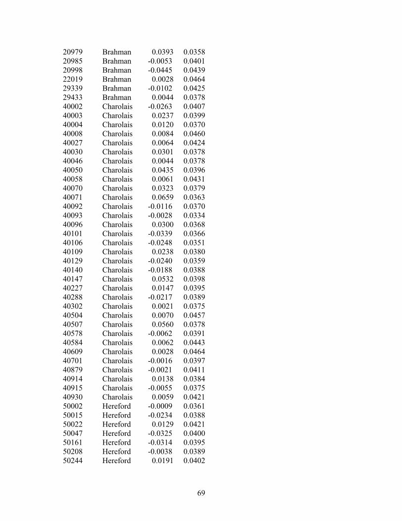
69

20979 Brahman 0.0393 0.0358 20985 Brahman -0.0053 0.0401 20998 Brahman -0.0445 0.0439 22019 Brahman 0.0028 0.0464 29339 Brahman -0.0102 0.0425 29433 Brahman 0.0044 0.0378 40002 Charolais -0.0263 0.0407 40003 Charolais 0.0237 0.0399 40004 Charolais 0.0120 0.0370 40008 Charolais 0.0084 0.0460 40027 Charolais 0.0064 0.0424 40030 Charolais 0.0301 0.0378 40046 Charolais 0.0044 0.0378 40050 Charolais 0.0435 0.0396 40058 Charolais 0.0061 0.0431 40070 Charolais 0.0323 0.0379 40071 Charolais 0.0659 0.0363 40092 Charolais -0.0116 0.0370 40093 Charolais -0.0028 0.0334 40096 Charolais 0.0300 0.0368 40101 Charolais -0.0339 0.0366 40106 Charolais -0.0248 0.0351 40109 Charolais 0.0238 0.0380 40129 Charolais -0.0240 0.0359 40140 Charolais -0.0188 0.0388 40147 Charolais 0.0532 0.0398 40227 Charolais 0.0147 0.0395 40288 Charolais -0.0217 0.0389 40302 Charolais 0.0021 0.0375 40504 Charolais 0.0070 0.0457 40507 Charolais 0.0560 0.0378 40578 Charolais -0.0062 0.0391 40584 Charolais 0.0062 0.0443 40609 Charolais 0.0028 0.0464 40701 Charolais -0.0016 0.0397 40879 Charolais -0.0021 0.0411 40914 Charolais 0.0138 0.0384 40915 Charolais -0.0055 0.0375 40930 Charolais 0.0059 0.0421 50002 Hereford -0.0009 0.0361 50015 Hereford -0.0234 0.0388 50022 Hereford 0.0129 0.0421 50047 Hereford -0.0325 0.0400 50161 Hereford -0.0314 0.0395 50208 Hereford -0.0038 0.0389 50244 Hereford 0.0191 0.0402

70

50251 Hereford 0.0051 0.0409 50366 Hereford 0.0086 0.0380 50368 Hereford -0.0667 0.0388 50411 Hereford -0.0056 0.0417 50419 Hereford 0.0377 0.0394 50423 Hereford -0.0088 0.0374 50459 Hereford 0.0099 0.0417 50463 Hereford -0.0395 0.0404 50601 Hereford 0.0117 0.0377 50631 Hereford 0.0026 0.0379 50635 Hereford -0.0418 0.0385 50700 Hereford 0.0076 0.0407 50738 Hereford 0.0169 0.0404 50767 Hereford -0.0099 0.0464 50789 Hereford -0.0359 0.0368 50849 Hereford -0.0010 0.0417 50933 Hereford 0.0153 0.0396 51107 Hereford 0.0265 0.0400 55101 Hereford -0.0244 0.0411 55133 Hereford 0.0213 0.0357 56105 Hereford 0.0050 0.0415 56138 Hereford -0.0074 0.0417 56144 Hereford 0.0040 0.0418 58212 Hereford -0.0175 0.0392 59221 Hereford -0.0238 0.0419

a, b, c = The breed of the cow exposed to the sire, expected progeny difference, and standard error or prediction error variance, respectively.

71

Appendix Table B. Expected progeny differences of sires for calf survival predicted from a normal model. Sire CSa EPDb StdErrc 10001 Angus 0.0048 0.0296 10003 Angus 0.0154 0.0304 10005 Angus 0.0041 0.0299 10010 Angus 0.0169 0.0296 10013 Angus -0.0042 0.0311 10020 Angus 0.0072 0.0310 10025 Angus 0.0038 0.0337 10047 Angus 0.0253 0.0281 10055 Angus -0.0001 0.0274 10068 Angus 0.0165 0.0273 10069 Angus 0.0147 0.0312 10084 Angus 0.0110 0.0331 10087 Angus -0.0006 0.0274 10100 Angus 0.0116 0.0323 10101 Angus 0.0006 0.0270 10111 Angus 0.0014 0.0340 10121 Angus 0.0039 0.0282 10139 Angus 0.0165 0.0286 10161 Angus 0.0037 0.0340 10194 Angus 0.0343 0.0266 10264 Angus 0.0230 0.0291 10273 Angus 0.0147 0.0285 10305 Angus 0.0312 0.0267 10313 Angus -0.0086 0.0330 10327 Angus 0.0180 0.0276 10348 Angus 0.0025 0.0284 10362 Angus 0.0013 0.0337 10368 Angus 0.0036 0.0305 10386 Angus 0.0020 0.0322 10416 Angus -0.0078 0.0258 10428 Angus 0.0192 0.0283 10437 Angus -0.0088 0.0307 10547 Angus 0.0018 0.0337 10586 Angus 0.0199 0.0287 10671 Angus 0.0024 0.0337 10673 Angus 0.0393 0.0289 10750 Angus -0.0026 0.0316 10779 Angus -0.0289 0.0301 10791 Angus 0.0060 0.0323 10792 Angus -0.0135 0.0321 10826 Angus 0.0204 0.0322 11375 Angus 0.0028 0.0340 15007 Angus 0.0234 0.0301

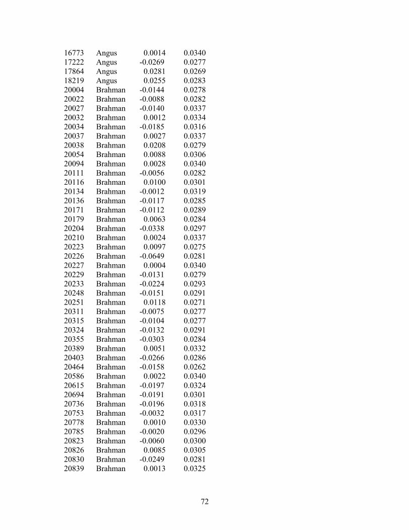
72

16773 Angus 0.0014 0.0340 17222 Angus -0.0269 0.0277 17864 Angus 0.0281 0.0269 18219 Angus 0.0255 0.0283 20004 Brahman -0.0144 0.0278 20022 Brahman -0.0088 0.0282 20027 Brahman -0.0140 0.0337 20032 Brahman 0.0012 0.0334 20034 Brahman -0.0185 0.0316 20037 Brahman 0.0027 0.0337 20038 Brahman 0.0208 0.0279 20054 Brahman 0.0088 0.0306 20094 Brahman 0.0028 0.0340 20111 Brahman -0.0056 0.0282 20116 Brahman 0.0100 0.0301 20134 Brahman -0.0012 0.0319 20136 Brahman -0.0117 0.0285 20171 Brahman -0.0112 0.0289 20179 Brahman 0.0063 0.0284 20204 Brahman -0.0338 0.0297 20210 Brahman 0.0024 0.0337 20223 Brahman 0.0097 0.0275 20226 Brahman -0.0649 0.0281 20227 Brahman 0.0004 0.0340 20229 Brahman -0.0131 0.0279 20233 Brahman -0.0224 0.0293 20248 Brahman -0.0151 0.0291 20251 Brahman 0.0118 0.0271 20311 Brahman -0.0075 0.0277 20315 Brahman -0.0104 0.0277 20324 Brahman -0.0132 0.0291 20355 Brahman -0.0303 0.0284 20389 Brahman 0.0051 0.0332 20403 Brahman -0.0266 0.0286 20464 Brahman -0.0158 0.0262 20586 Brahman 0.0022 0.0340 20615 Brahman -0.0197 0.0324 20694 Brahman -0.0191 0.0301 20736 Brahman -0.0196 0.0318 20753 Brahman -0.0032 0.0317 20778 Brahman 0.0010 0.0330 20785 Brahman -0.0020 0.0296 20823 Brahman -0.0060 0.0300 20826 Brahman 0.0085 0.0305 20830 Brahman -0.0249 0.0281 20839 Brahman 0.0013 0.0325

73

20853 Brahman -0.0023 0.0308 20863 Brahman -0.0005 0.0306 20869 Brahman 0.0059 0.0326 20893 Brahman 0.0101 0.0302 20924 Brahman -0.0046 0.0280 20926 Brahman -0.0286 0.0276 20927 Brahman -0.0072 0.0281 20930 Brahman 0.0021 0.0314 20931 Brahman 0.0186 0.0304 20951 Brahman -0.0343 0.0302 20962 Brahman -0.0276 0.0308 20979 Brahman 0.0278 0.0286 20985 Brahman 0.0074 0.0313 20998 Brahman -0.0044 0.0328 22019 Brahman 0.0011 0.0340 29339 Brahman -0.0179 0.0281 29433 Brahman 0.0040 0.0273 40002 Charolais -0.0195 0.0298 40003 Charolais -0.0090 0.0285 40004 Charolais 0.0076 0.0271 40006 Charolais 0.0035 0.0337 40008 Charolais -0.0155 0.0330 40010 Charolais 0.0037 0.0340 40024 Charolais 0.0033 0.0340 40025 Charolais -0.0113 0.0340 40027 Charolais -0.0358 0.0305 40030 Charolais -0.0549 0.0277 40035 Charolais -0.0087 0.0335 40046 Charolais -0.0166 0.0277 40050 Charolais 0.0074 0.0276 40051 Charolais 0.0053 0.0332 40058 Charolais 0.0100 0.0310 40068 Charolais -0.0080 0.0302 40070 Charolais 0.0019 0.0301 40071 Charolais 0.0132 0.0297 40092 Charolais 0.0040 0.0277 40093 Charolais 0.0347 0.0269 40096 Charolais 0.0071 0.0283 40101 Charolais -0.0366 0.0264 40106 Charolais 0.0165 0.0273 40109 Charolais -0.0130 0.0273 40125 Charolais 0.0040 0.0314 40129 Charolais -0.0146 0.0268 40140 Charolais -0.0262 0.0266 40147 Charolais 0.0019 0.0302 40227 Charolais -0.0411 0.0279

74

40288 Charolais 0.0249 0.0307 40302 Charolais -0.0098 0.0291 40504 Charolais 0.0006 0.0340 40507 Charolais 0.0163 0.0303 40578 Charolais 0.0098 0.0284 40584 Charolais 0.0104 0.0326 40701 Charolais 0.0206 0.0283 40879 Charolais 0.0029 0.0310 40914 Charolais -0.0033 0.0285 40915 Charolais 0.0069 0.0283 40930 Charolais 0.0018 0.0309 50001 Hereford 0.0033 0.0337 50002 Hereford -0.0136 0.0289 50008 Hereford 0.0000 0.0312 50015 Hereford 0.0202 0.0275 50022 Hereford 0.0128 0.0313 50024 Hereford 0.0061 0.0335 50036 Hereford 0.0120 0.0289 50040 Hereford 0.0008 0.0340 50042 Hereford 0.0064 0.0335 50046 Hereford 0.0010 0.0340 50047 Hereford -0.0339 0.0295 50067 Hereford 0.0099 0.0293 50102 Hereford 0.0068 0.0330 50131 Hereford 0.0268 0.0303 50144 Hereford -0.0012 0.0324 50149 Hereford -0.0127 0.0315 50161 Hereford 0.0028 0.0310 50208 Hereford 0.0181 0.0274 50214 Hereford -0.0151 0.0317 50232 Hereford -0.0063 0.0332 50244 Hereford 0.0015 0.0312 50251 Hereford 0.0204 0.0307 50366 Hereford 0.0049 0.0281 50368 Hereford -0.0026 0.0278 50369 Hereford 0.0122 0.0316 50411 Hereford 0.0125 0.0308 50419 Hereford -0.0086 0.0289 50423 Hereford 0.0014 0.0281 50459 Hereford 0.0174 0.0317 50463 Hereford 0.0009 0.0283 50601 Hereford -0.0361 0.0283 50631 Hereford -0.0187 0.0282 50635 Hereford -0.0063 0.0286 50700 Hereford 0.0112 0.0289 50738 Hereford 0.0004 0.0307

75

50787 Hereford 0.0028 0.0340 50789 Hereford -0.0178 0.0293 50796 Hereford 0.0015 0.0337 50849 Hereford -0.0146 0.0274 50869 Hereford -0.0021 0.0330 50933 Hereford 0.0152 0.0272 51019 Hereford 0.0074 0.0330 51107 Hereford 0.0175 0.0310 55101 Hereford 0.0055 0.0284 55133 Hereford 0.0118 0.0279 56044 Hereford 0.0067 0.0281 56105 Hereford 0.0173 0.0310 56138 Hereford 0.0046 0.0310 56144 Hereford 0.0139 0.0310 58212 Hereford 0.0105 0.0273 58919 Hereford 0.0000 0.0339 59221 Hereford 0.0061 0.0311 80004 Gelbvieh -0.0145 0.0272 80005 Gelbvieh -0.0090 0.0337 80006 Gelbvieh 0.0069 0.0308 80007 Gelbvieh -0.0071 0.0332 80012 Gelbvieh 0.0023 0.0315 80048 Gelbvieh -0.0027 0.0312 80082 Gelbvieh 0.0269 0.0296 80108 Gelbvieh -0.0334 0.0281 80224 Gelbvieh 0.0065 0.0330 80256 Gelbvieh 0.0055 0.0328 80270 Gelbvieh -0.0103 0.0319 80276 Gelbvieh 0.0088 0.0319 80280 Gelbvieh 0.0010 0.0340 80282 Gelbvieh 0.0140 0.0325 80327 Gelbvieh 0.0008 0.0312 80408 Gelbvieh -0.0126 0.0340 90001 Simmental -0.0118 0.0334 90004 Simmental -0.0179 0.0328 90005 Simmental 0.0030 0.0332 90006 Simmental 0.0018 0.0337 90007 Simmental 0.0037 0.0337 90008 Simmental 0.0030 0.0337 90009 Simmental 0.0026 0.0337 90010 Simmental 0.0027 0.0334 90011 Simmental 0.0086 0.0325 90012 Simmental -0.0026 0.0296 90013 Simmental 0.0058 0.0330 90014 Simmental 0.0033 0.0330 90015 Simmental 0.0022 0.0337

76

90016 Simmental 0.0029 0.0337 90017 Simmental 0.0002 0.0334 90033 Simmental 0.0271 0.0276 90034 Simmental -0.0129 0.0310 90104 Simmental -0.0124 0.0316 90189 Simmental -0.0011 0.0314 90403 Simmental -0.0122 0.0286 90404 Simmental -0.0127 0.0339 90435 Simmental 0.0003 0.0279 90498 Simmental 0.0041 0.0309 90531 Simmental 0.0064 0.0328 90716 Simmental 0.0054 0.0328 90810 Simmental 0.0017 0.0337 91004 Simmental 0.0002 0.0340 91009 Simmental -0.0023 0.0321 91016 Simmental 0.0021 0.0340 91614 Simmental -0.0096 0.0335 91615 Simmental 0.0021 0.0337

a, b, c = The breed of the cow exposed to the sire, expected progeny difference, and standard error or prediction error variance, respectively.

77

Appendix Table C. The SAS program to estimate genetic parameters /*This procedure invokes the GLIMMIX macro in SAS.*/ dm 'log;clear;output;clear'; %inc 'glmm800.sas' / nosource; run; /*The codes shown below for the GLIMMIX syntax are used to run an analysis with cow age (age) as a class variable, calf birth weight (calfbwtk) as a continuous covariable, and sire as random variable. No comas or parenthesis can be changed. The reml statement requests the quasi-likelihood methodology to be used. The covest statement tests the sire component of variance for statistical significance.*/ %glimmix (data=csmain, procopt=method=reml covtest, stmts=%str( class age sire; model cs= age calfbwtk; random sire ; /*The codes shown below below are used to simulate a Markov chain with 10,000 samples based on an independence sampling algorithm with a default noninformative prior. The nsample statement determines the size of the chain. The seed statement determines the starting point of the chain. The Markov chain is outputted as the data set normal in the work library of SAS.*/ prior / nsample=1e4 lognote=1e4 seed=10455575770 psearch ptrans out=normal;), /* The codes below specified the generalized mixed model that is to be used. The error term determines the assumed distribution and the link statement specifies the link function that GLIMMIX will use. The statements shown runs a linear model.*/ error=normal, link=identity); run; /*The following data step codes creates heritability in the normal data set.*/ data normal;set normal; heritability=4*covp1/(covp1+covp2); run; /*The following codes in SAS are used to estimate the moments of the posterior distribution simulated by the GLIMMIX macro with the kernel procedures of SAS. The

78

data set used is the normal data set. The other statements deal with setting up the instructions for building the graph of the posterior distribution.*/ proc kde data=normal out=dena ng=100 method=srot bwm=1.5; var heritability; where heritability <10; symbol i=join; run; /*The following statements are used to produce graphs of the posterior distribution. The data set used is the dena that was created by the proc kde procedure.*/ proc gplot data=dena; plot density*heritability; run; /*Additional information can be found in Littell et al. (1996) and at www.id.unizh.ch/software/unix/statmath/sas/sasdoc/stat/chap41/index.htm.*/

79

VITA

Jose Lucio Lima Guerra, a native of Fortaleza, state of Ceara - Brazil, was born

January 6, 1973. He graduated from Geo Studio High School in Fortaleza in 1991. He

earned a Bachelor of Science degree in 1998 in Louisiana State University, Baton Rouge,

Louisiana. In 1998 he began a master’s program in beef cattle in the Animal Science

Department of the Louisiana State University. He earned a Master of Science degree in

2000. In 2000 he began a doctoral program with a minor in applied statistics. He is now

a candidate for the Doctor of philosophy degree in the interdepartmental program of

animal, dairy, and poultry sciences.