Statistical Modeling of Text (Can be seen as an application of probabilistic graphical models) Best...

Statistical Modeling of Text

(Can be seen as an application of probabilistic graphical models)

Best reading supplement for just LDA : http://rakaposhi.eas.asu.edu/cse571/lda-lsa-reading.pdf

(the original JMLR paper by Blei et al is also good)

http://rakaposhi.eas.asu.edu/cse571/lda-lsa-reading.pdf



Modeling Text Documents• Documents are sequences are words

– D = [p1=w1 p2=w2 p3=w3 … pk=wk] • Where wi are drawn from some vocabulary V

– So P(D) = P([p1=w1 p2=w2 p3=w3 … pk=wk])– Needs too many joint probabilities.. How many?

• If the vocabulary size is 10K, and there are 5K words in each novel, then we need 10K^5K joint probabilities– There are at most 10K novels in English..

• Let us make assumptions

Unigram Model• Assume that all words occur independently

(!)P(pi=wi pk=wk) = P(pi=wi)*P(pk=wk)

P(pi=wi pk=wi) = P(pi=wi)*P(pi=wi)

– P ([p1=w1 p2=w2 p3=w3 … pk=wk]) = P(w1)#(w1) P(w2)#(w2) …

Note that this way the probability of occurrence of a word is the same in EVERY DOCUMENT… --A little too overboard.. --words in neighboring positions tend to be correlated (bigram models; trigram models) --Different documents tend to have different topics… topic models

Single Topic Model• Assume each document has a topic z• The topic z determines the probabilities of the

word occurrence– P ([p1=w1 p2=w2 p3=w3 … pk=wk]|z) = P(w1|

z)#(w1) P(w2|z)#(w2) …

The “supervised” version of this model is the Naïve Bayes classifier

Connection to candies? lime and cherry are words bag types (h1..h5) are topics you see candies; you guess bag types..

Topic is just a distribution over words!

HEART 0.2 LOVE 0.2SOUL 0.2TEARS 0.2JOY 0.2SCIENTIFIC 0.0KNOWLEDGE 0.0WORK 0.0RESEARCH 0.0MATHEMATICS 0.0

HEART 0.0 LOVE 0.0SOUL 0.0TEARS 0.0JOY 0.0 SCIENTIFIC 0.2KNOWLEDGE 0.2WORK 0.2RESEARCH 0.2MATHEMATICS 0.2

topic 1 topic 2

w P(w|Cat = 1) w P(w|Cat = 2)

Viewing Topic Learning as BN Learning

• Note that we are given the topology!• So we only need to learn parameters• Two cases:

– Case 1: We are given a bunch of novels, and their topics• Naïve Bayes!

– Case 2: We are just given a bunch of novels, but no topics• Incomplete Data; EM algorithm (if doing

MLE)– What is EM optimizing?

» Consider Harcopy/Softcopy division vs. Westerns/Chick-Lit/SciFi topics

Unsupervised vs. Supervised is just complete data vs incomplete data!!

Topic Models and Dimensionality reduction

• Suppose I have a document d with me. What information do you need from me so you can reconstruct that document (statistically speaking)?– In the unigram case, you don’t need any information from

me; you can generate your version of the document with the word distribution

– In the single topic case, you need me to tell you the topic – In the multi-topic case, you need me to tell you the

mixture over the k topics (k probabilities)

• Notice that this way, we are compressing the document down! (to zero, one or k-bits of information!—The rest are just details)

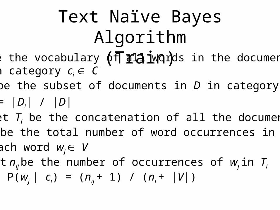
Text Naïve Bayes Algorithm(Train)

Let V be the vocabulary of all words in the documents in DFor each category ci C

Let Di be the subset of documents in D in category ci

P(ci) = |Di| / |D|

Let Ti be the concatenation of all the documents in Di

Let ni be the total number of word occurrences in Ti

For each word wj V Let nij be the number of occurrences of wj in Ti

Let P(wj | ci) = (nij + 1) / (ni + |V|)

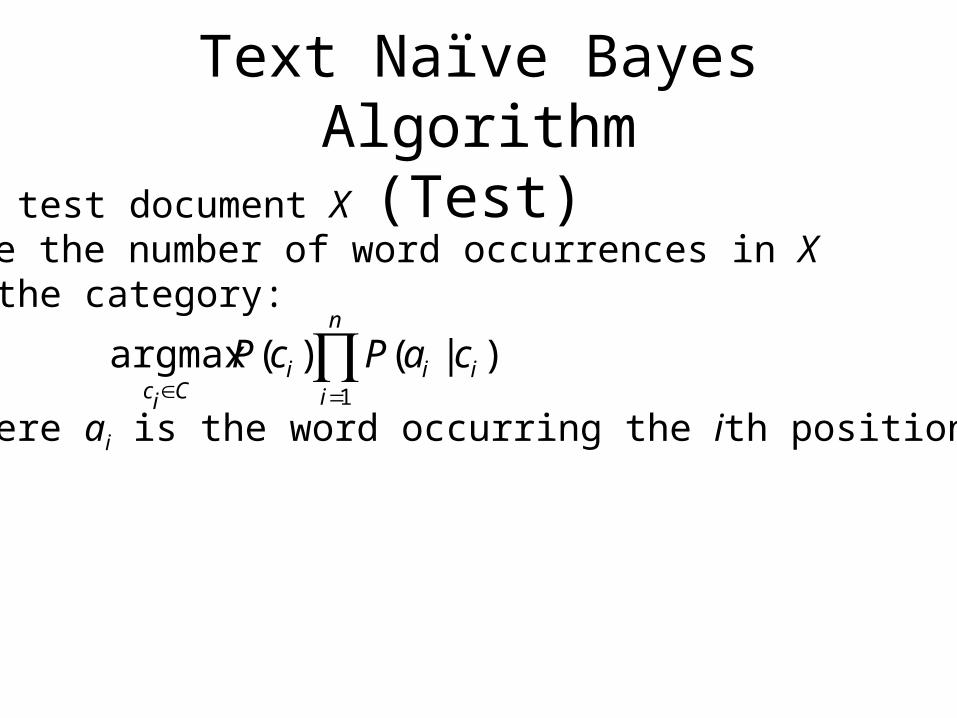
Text Naïve Bayes Algorithm(Test)

Given a test document XLet n be the number of word occurrences in XReturn the category:

where ai is the word occurring the ith position in X

)|()(argmax1

n

iiii

CiccaPcP

Bayesian document categorization

Cat

w1nD

D

priors

P(w|Cat)

P(Cat)

Wait—What do you LEARN here? Nothing..But then how are the probabilities set? By sampling from the priorBut how does data change anything? By changing the posteriorSo you don’t estimate any parameters? NoYou just do inference? Yes..

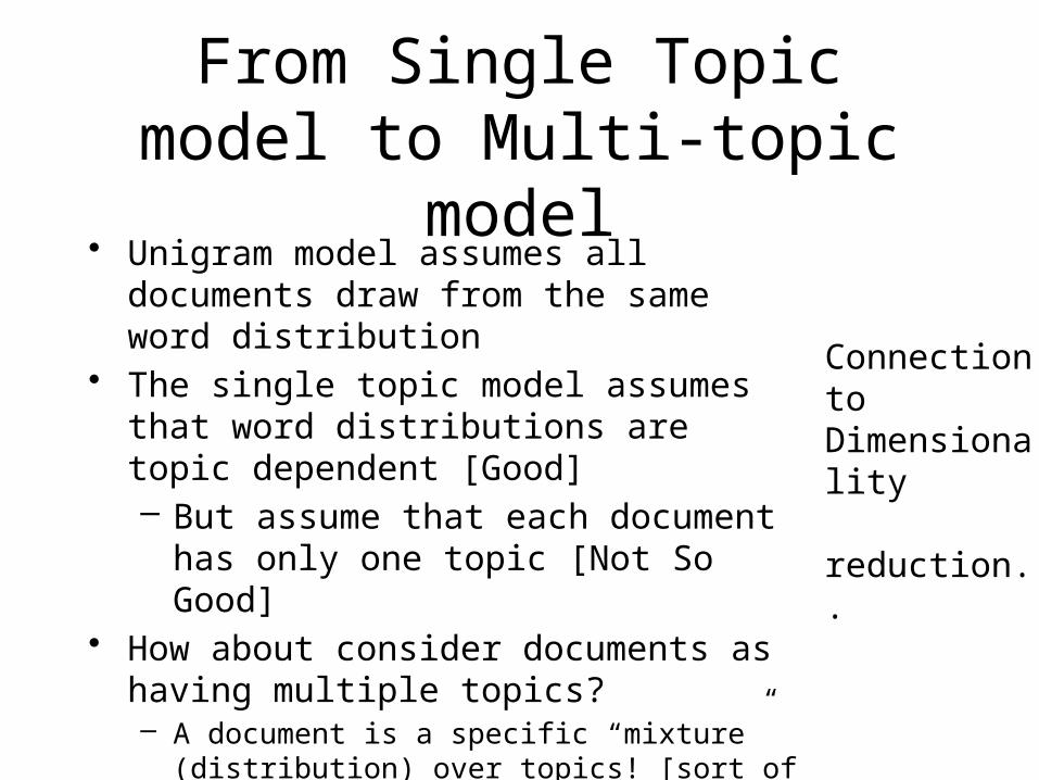
From Single Topic model to Multi-topic model

• Unigram model assumes all documents draw from the same word distribution

• The single topic model assumes that word distributions are topic dependent [Good]– But assume that each document has only one

topic [Not So Good]• How about consider documents as having

multiple topics?– A document is a specific “mixture” (distribution) over

topics! [sort of like belief states ;-] – In the single topic case, the “mixture” is a degenerate

one—with all probability mass on just one topic

Connection toDimensionality reduction..

Intuition behind LDA

[LDA slides from Blei’s MLSS 09 lecture]

Generative model

Note that we are assuming that contiguous words may come from different topics!

Importance of the “sparsity” We want a document to have more than one topic, but not really all the topics.. You can ensureSparsity by starting witha dirichlet prior whoseHyper parameter sum isLow..

(you get interesting colors by combining primary colors, but if you combine them all you always get white..)

See http://cs.stanford.edu/people/karpathy/nipspreview/ for an exampleOn NIPS papers

http://cs.stanford.edu/people/karpathy/nipspreview/

The posterior distribution

Unrolled LDA Model

z4z3z2z1

w4w3w2w1

b

z4z3z2z1

w4w3w2w1

z4z3z2z1

w4w3w2w1

For each document, Choose ~Dirichlet() For each of the N words wn:

Choose a topic zn» Multinomial() Choose a word wn from p(wn|zn,), a multinomial

probability conditioned on the topic zn.

LDA modelLDA as a dimensionality reduction algorithm

--Documents can be seen as vectors in k-dimenstional topic space--as against V-dimensional vocabulary space

Why sum over Zn? Because the same word might have come due to different topics…

Dirichlet distribution

Dirichlet Examples

Darker implies lower magnitude

\alpha < 1 leads to sparser topics

A generative model for documents

HEART 0.2 LOVE 0.2SOUL 0.2TEARS 0.2JOY 0.2SCIENTIFIC 0.0KNOWLEDGE 0.0WORK 0.0RESEARCH 0.0MATHEMATICS 0.0

HEART 0.0 LOVE 0.0SOUL 0.0TEARS 0.0JOY 0.0 SCIENTIFIC 0.2KNOWLEDGE 0.2WORK 0.2RESEARCH 0.2MATHEMATICS 0.2

topic 1 topic 2

w P(w|Cat = 1) w P(w|Cat = 2)

Choose mixture weights for each document, generate “bag of words”

{P(z = 1), P(z = 2)}

{0, 1}

{0.25, 0.75}

{0.5, 0.5}

{0.75, 0.25}

{1, 0}

MATHEMATICS KNOWLEDGE RESEARCH WORK MATHEMATICS RESEARCH WORK SCIENTIFIC MATHEMATICS WORK

SCIENTIFIC KNOWLEDGE MATHEMATICS SCIENTIFIC HEART LOVE TEARS KNOWLEDGE HEART

MATHEMATICS HEART RESEARCH LOVE MATHEMATICS WORK TEARS SOUL KNOWLEDGE HEART

WORK JOY SOUL TEARS MATHEMATICS TEARS LOVE LOVE LOVE SOUL

TEARS LOVE JOY SOUL LOVE TEARS SOUL SOUL TEARS JOY

LDA modelLDA as a dimensionality reduction algorithm

--Documents can be seen as vectors in k-dimenstional topic space--as against V-dimensional vocabulary space

Why sum over Zn? Because the same word might have come due to different topics…

Inverting the generative model

• Maximum likelihood or MAP estimation (EM)– e.g. Hofmann (1999)

• Bayesian Estimation– Compute the posteriors P( |q d) P(b| d)

• We know P(q) and P(b) [They are set by Dirichlet]• Use bayesian updating to compute P( |q w,d) P(b|w,d)

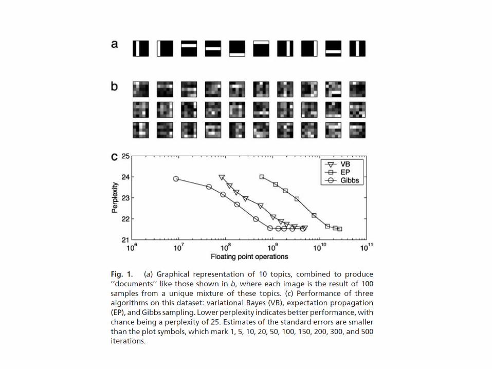
– Deterministic approximate algorithms • variational EM; Blei, Ng & Jordan (2001; 2003)• expectation propagation; Minka & Lafferty (2002)

– Markov chain Monte Carlo• Full Gibbs sampler; Pritchard et al. (2000)

– Estimates P(• collapsed Gibbs sampler; Griffiths & Steyvers (2004)

Unrolled LDA Model

z4z3z2z1

w4w3w2w1

b

z4z3z2z1

w4w3w2w1

z4z3z2z1

w4w3w2w1

For each document, Choose ~Dirichlet() For each of the N words wn:

Choose a topic zn» Multinomial() Choose a word wn from p(wn|zn,), a multinomial

probability conditioned on the topic zn.

Note that the other parents of zj are part of the markov blanket

P(rain|cl,sp,wg) = P(rain|cl) * P(wg|sp,rain)

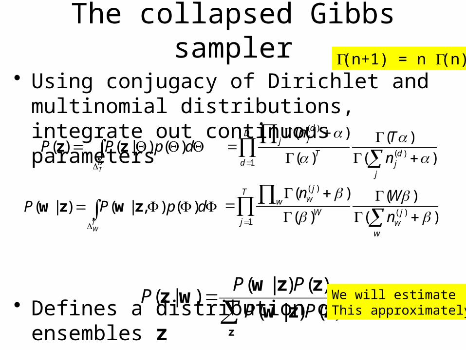
The collapsed Gibbs sampler

• Using conjugacy of Dirichlet and multinomial distributions, integrate out continuous parameters

• Defines a distribution on discrete ensembles z

dpPPTW

)(),|()|( zwzw

dpPPDT

)()|()( zz

z

zzw

zzwwz

)()|(

)()|()|(

PP

PPP

T

jw

jw

Ww

jw

n

Wn

1)(

)(

)(

)(

)(

)(

D

dj

dj

T

j

dj

n

Tn

1)(

)(

)(

)(

)(

)(

G(n+1) = n G(n)

We will estimateThis approximately

The LDA model is no longer sparse after marginalization….! But you don’t need to see it ;-) unroll

Marginalize

Bayesians are the only people who feel marginalized when integrated..

Viewing the “integrating out” Graphically

We can do Gibbs sampling withoutIntegrating.. It will be inefficient..

Compare markov blankets for qij

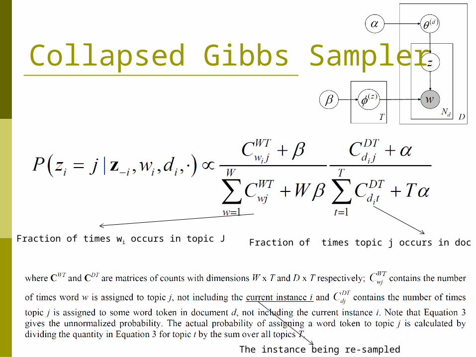
Collapsed Gibbs Sampler

The instance being re-sampled

Fraction of times wi occurs in topic J Fraction of times topic j occurs in doc di

Gibbs sampling in LDA

i wi di zi123456789

101112...

50

MATHEMATICSKNOWLEDGE

RESEARCHWORK

MATHEMATICSRESEARCH

WORKSCIENTIFIC

MATHEMATICSWORK

SCIENTIFICKNOWLEDGE

.

.

.JOY

111111111122...5

221212212111...2

iteration1

5 docs; 10 words/doc; 2 topics


i wi di zi zi123456789

101112...

50


RESEARCHWORK

MATHEMATICSRESEARCH

WORKSCIENTIFIC

MATHEMATICSWORK

SCIENTIFICKNOWLEDGE

.

.

.JOY

111111111122...5

221212212111...2

?

iteration1 2



101112...

50


RESEARCHWORK

MATHEMATICSRESEARCH

WORKSCIENTIFIC

MATHEMATICSWORK

SCIENTIFICKNOWLEDGE

.

.

.JOY

111111111122...5

221212212111...2

2?

iteration1 2



101112...

50


RESEARCHWORK

MATHEMATICSRESEARCH

WORKSCIENTIFIC

MATHEMATICSWORK

SCIENTIFICKNOWLEDGE

.

.

.JOY

111111111122...5

221212212111...2

21?

iteration1 2



101112...

50


RESEARCHWORK

MATHEMATICSRESEARCH

WORKSCIENTIFIC

MATHEMATICSWORK

SCIENTIFICKNOWLEDGE

.

.

.JOY

111111111122...5

221212212111...2

211?

iteration1 2



101112...

50


RESEARCHWORK

MATHEMATICSRESEARCH

WORKSCIENTIFIC

MATHEMATICSWORK

SCIENTIFICKNOWLEDGE

.

.

.JOY

111111111122...5

221212212111...2

2112?

iteration1 2


i wi di zi zi zi123456789

101112...

50


RESEARCHWORK

MATHEMATICSRESEARCH

WORKSCIENTIFIC

MATHEMATICSWORK

SCIENTIFICKNOWLEDGE

.

.

.JOY

111111111122...5

221212212111...2

211222212212...1

…

222122212222...1

iteration1 2 … 1000

Can estimateP(Z|W)

Recovering j and q

Probability of ith word in jth topic Probability of jth topic doc d

Marginalization

Gibbs Sampling

Recovering j and q

Once you have topics, not all documents are generatable!

LDA (like any generative model) is modular, general, useful

58

Event Tweet Alignment..Republican Primary Debate, 09/07/2011 Tweets tagged with #ReaganDebate

?

?

Which part of the event did a tweet refer to?What were the topics of the event and tweets?

Applications: Event playback/Analysis, Sentiment Analysis, Advertisement, etc

Yuheng

GOP Primary debate on Sept 07, 2011, talked about various issues such as job creation, healthcare, foreign policy, etcwe crawled tweet using the official hashtag, posted by NBC newsWith vast amount of tweets, we want to know two things: 1) which part of the event did a tweet refer to and 2)what were the topicsAnswering two questions has great applications, e.g., event analysis, playback, situation awareness etc

Event-Tweet Alignment: The Problem

• Given an event’s transcript S and its associated tweets T– Find the segment s (s ∈ S) which is topically

referred by tweet t (t ∈ T) [Could be a general tweet]

• Alignment requires:1. Extracting topics in the tweets and event2. Segmenting the event into topically coherent chunks3. Classify the tweets

--General vs. Specific

5959

Idea: represent tweets and segements in a topic space

Yuheng

Here's a conceptual model of tweet and event.event has segment, tweets can be either general or specific, if general, then it can refer to whole event, otherwise, it can refer to centain specific segment, in any case, such reference is based on topics.

60

Event-Tweet Alignment: A Model

Event-Tweet Alignment: Challenges

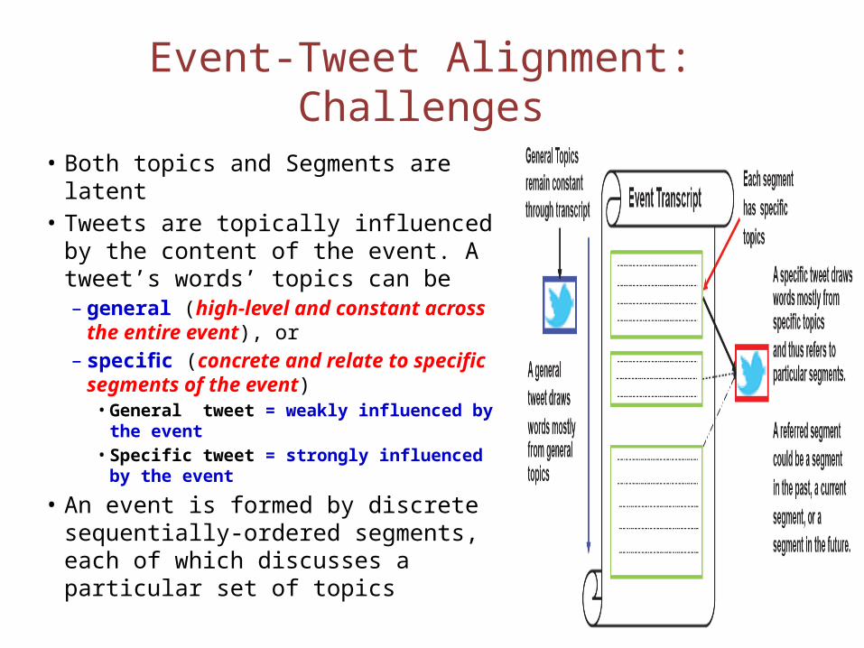
• Both topics and Segments are latent

• Tweets are topically influenced by the content of the event. A tweet’s words’ topics can be – general (high-level and constant

across the entire event), or– specific (concrete and relate to

specific segments of the event)• General tweet = weakly influenced

by the event• Specific tweet = strongly influenced

by the event

• An event is formed by discrete sequentially-ordered segments, each of which discusses a particular set of topics

61

ET-LDA

63

ET-LDA ModelEvent Tweets

Determine event segmentation

Determine tweet type

Determine which segment a tweet (word) refers to

Determine word’s topic in event Tweets

word’s topic

64

Yuheng

in the event part, we assume that an event is formed by discrete sequentially-ordered segments, each of which discusses a particular set of topicsto do segmentatoin/model the topic evolutions in the event, we apply the Markov assumption on \theta(s),with some probability, it is as same asthe distribution of topics of previous paragraph s-1, otherwise, a new distribution of topics \theta(s) is sampled from a dirichlet. This pattern of dependency is produced by associating a binary variable c(s). with each paragraph, indicating whether its topic is the same as that of the previous paragraph or different. If the topic remains the same, these paragraphs are merged to form one segment.

Yuheng

we assume that a tweet consists ofwords which can belong to two distinct types of topics: general topics, which are high-level and constant across the entire event, and specific topics, which are detailed and relate to the segments of the event. As a result, the distribution of general topics is fixed for a tweet. However, the distribution of specific topics keeps varying with respect to the development of the event. each word in a tweet is associated with a distribution of topics. It can be either sampled from a mixture of specific topics \theta(s), or a mixture of general topics \psi(t) over K topicsdepending on a binary variable c(t) sampled from a binomial distribution. In the first case, \theta(s)is from a referring segment s of the event, where s is chosen according to a categorical distribution s(t). An important property of the categorical distribution s(t) is to allow choosing any segment in the event. This reflects the fact that a person may compose a tweet on topics discussed in a segment that (1) was in the past (2) is currently occurring, or (3) will occur after the tweet is posted (usually when she expects certain topics to be discussed in the event)

ET-LDA Model

65For more details of the inference, please refer to our paper: http://bit.ly/MBHjyZ

http://bit.ly/MBHjyZ



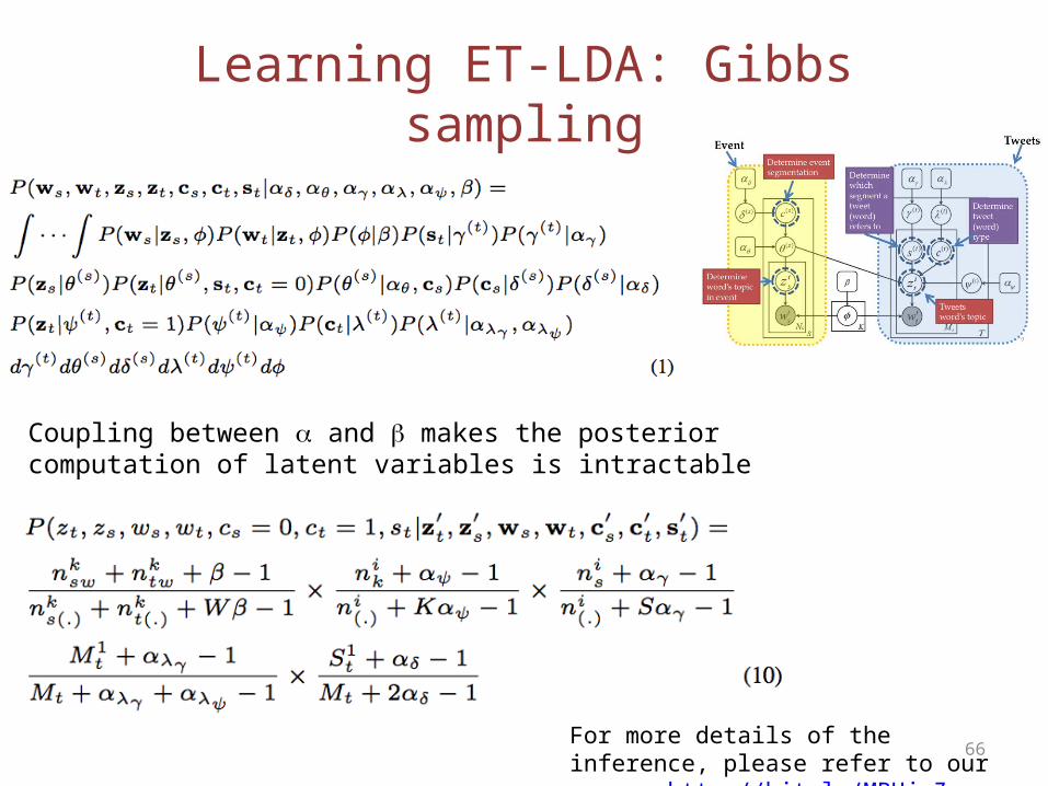
Learning ET-LDA: Gibbs sampling

66For more details of the inference, please refer to our paper: http://bit.ly/MBHjyZ

Coupling between a and b makes the posterior computation of latent variables is intractable




Analysis of the First Obama-Romney Debate

67

Generative vs. Discriminative Learning

• Often, we are really more interested in predicting only a subset of the attributes given the rest.– E.g. we have data attributes split into subsets X and Y, and we

are interested in predicting Y given the values of X • You can do this by either by

– learning the joint distribution P(X, Y) [Generative learning]– or learning just the conditional distribution P(Y|X)

[Discriminative learning]• Often a given classification problem can be handled either

generatively or discriminatively– E.g. Naïve Bayes and Logistic Regression

• Which is better?

Generative vs. Discriminative

Generative Learning• More general (after all if you have

P(Y, X) you can predict Y given X as well as do other inferences– You can predict jokes as well as

make them up (or predict spam mails as well as generate them)

• In trying to learn P(Y,X), we are often forced to make many independence assumptions both in Y and X—and these may be wrong..– Interestingly, this type of high bias

can help generative techniques when there is too little data

Discriminative Learning• More to the point (if what you want

is P(Y|X), why bother with P(Y,X) which is after all P(Y|X) *P(X) and thus models the dependencies between X’s also?

• Since we don’t need to model dependencies among X, we don’t need to make any independence assumptions among them. So, we can merrily use highly correlated features..– Interestingly, this freedom can hurt

discriminative learners when there is too little data (as over fitting is easy)

Bayes networks are not well suited for discriminative learning; Markov Networks are--thus Conditional Random Fields are basically MNs doing discriminative learning

--Logistic regression can be seen as a simple CRF

P(y)P(x|y) = P(y,x) = P(x)P(y|x)

Collapsed Gibbs Sampler

The instance being re-sampled

Fraction of times wi occurs in topic J Fraction of times topic j occurs in doc di

Statistical Modeling of Text (Can be seen as an application of probabilistic graphical models) Best...

Documents

Transcript of Statistical Modeling of Text (Can be seen as an application of probabilistic graphical models) Best...