Statistical NLP: Lecture 8 Statistical Inference: n-gram Models over Sparse Data (Ch 6)
Upload
trinhduongCategory
view
222download
0
1
Statistical Methods for NLP
Maximum Entropy Models
Sameer Maskey
Week 6, Feb 23, 2010
2
Topics for Today
� Logistic Regression/Maximum Entropy
Models

3
Project
� Feb 23, 2010 (11:59pm) : Project Proposal
� March 23, 2010 (4pm) : Project Status
Update
� April 20, 2010 (4pm) : Final Projects Due
� April 27, 2010 (4pm) : Class Presentations for
the project

4
Maximum Entropy Model
� Maximum Entropy Model has shown to perform well
in many NLP tasks
� POS tagging [Ratnaparkhi, A., 1996]
� Text Categorization [Nigam, K., et. al, 1999]
� Named Entity Detection [Borthwick, A, 1999]
� Parser [Charniak, E., 2000]
� Discriminative classifier
� Conditional model P(c|d)
� Maximize conditional likelihood
� Can handle variety of features

5
Naïve Bayes vs. Maximum Entropy Models
� Trained by maximizing likelihood of data and class
� Features are assumed independent
� Feature weights set independently
� Trained by maximizing conditional likelihood of classes
� Dependency on features taken account by feature weights
� Feature weights are set mutually
Naïve Bayes Model Maximum Entropy Model

6
Entropy
� Measure of uncertainty
� Higher uncertainty equals higher entropy
� Degree of surprise of an event
� Why this formula in particular? Why log?
H(p) = −∑
x
p(x)log2 p(x)

7
Exploring the Entropy Formulation
� How much information received when observing a random
variable ‘x’ ?
� Highly improbable event = received more information
� Highly probable event = received less information
� Need h(x) that express information content of p(x); we want
1. Monotonic function of p(x)
2. If p(x,y) = p(x). p(y) when x and y are unrelated, i.e. statistically
independent then we want h(x,y) = h(x) + h(y) such that
information gain by observing two unrelated events is their sum
8
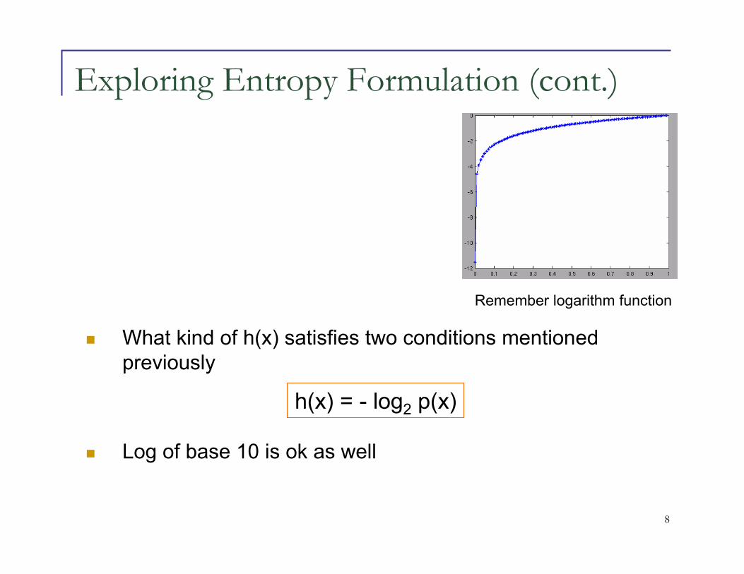
Exploring Entropy Formulation (cont.)
h(x) = - log2 p(x)
� What kind of h(x) satisfies two conditions mentioned
previously
� Log of base 10 is ok as well
Remember logarithm function
9
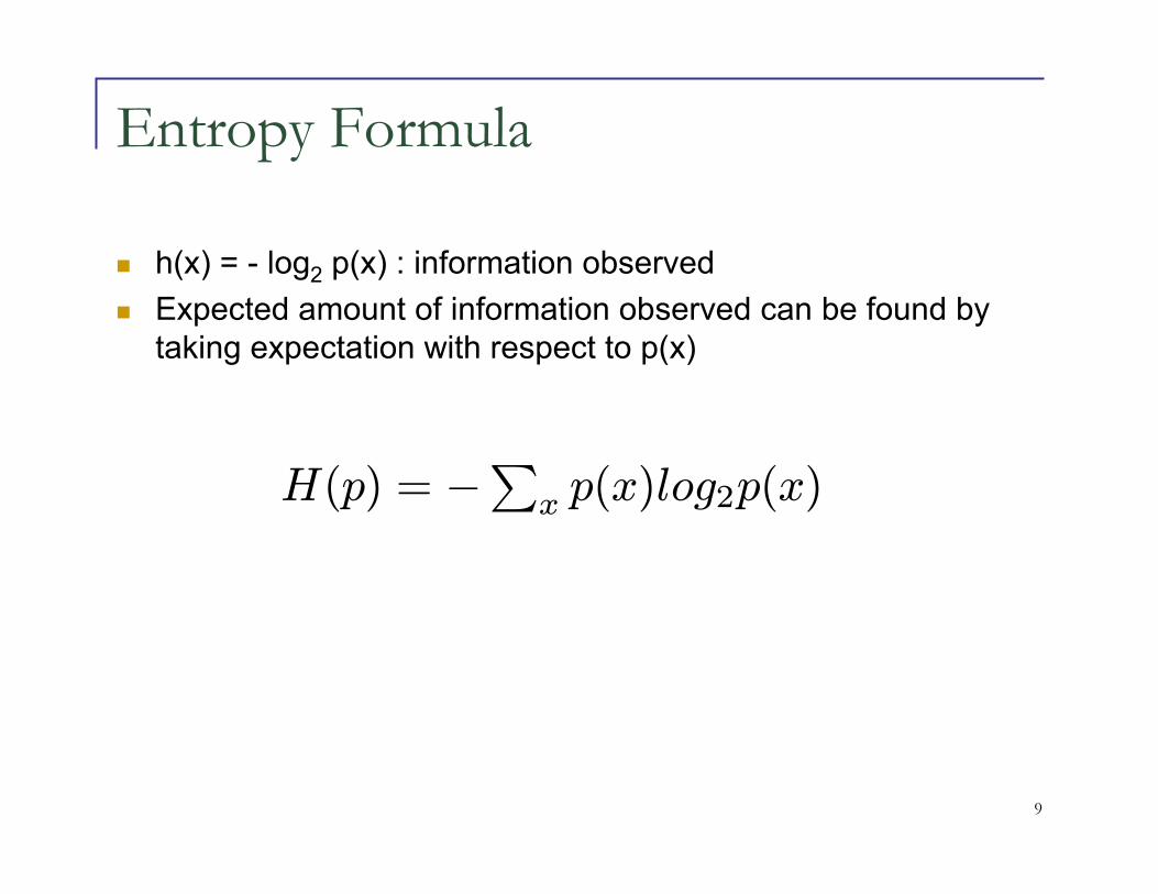
Entropy Formula
� h(x) = - log2 p(x) : information observed
� Expected amount of information observed can be found by
taking expectation with respect to p(x)
H(p) = −∑x p(x)log2p(x)

10
Comparing Entropy Across Distributions
[1] Uniform distribution has higher entropy

11
Maximizing Entropy
� How can we find a distribution with maximum entropy?
� What about maximizing entropy of a distribution with a set of constraints?
� What does maximizing entropy has to do with classification task anyway?
� Let us first look at logistic regression to understand this

12
Remember Linear Regression
� We estimated theta by setting square loss function’s
derivative to zero
yj = θ0 + θ1xj
yj =∑Ni=0 θixij where x0j = 1
N is the number of dimensions where
each input lives in
13
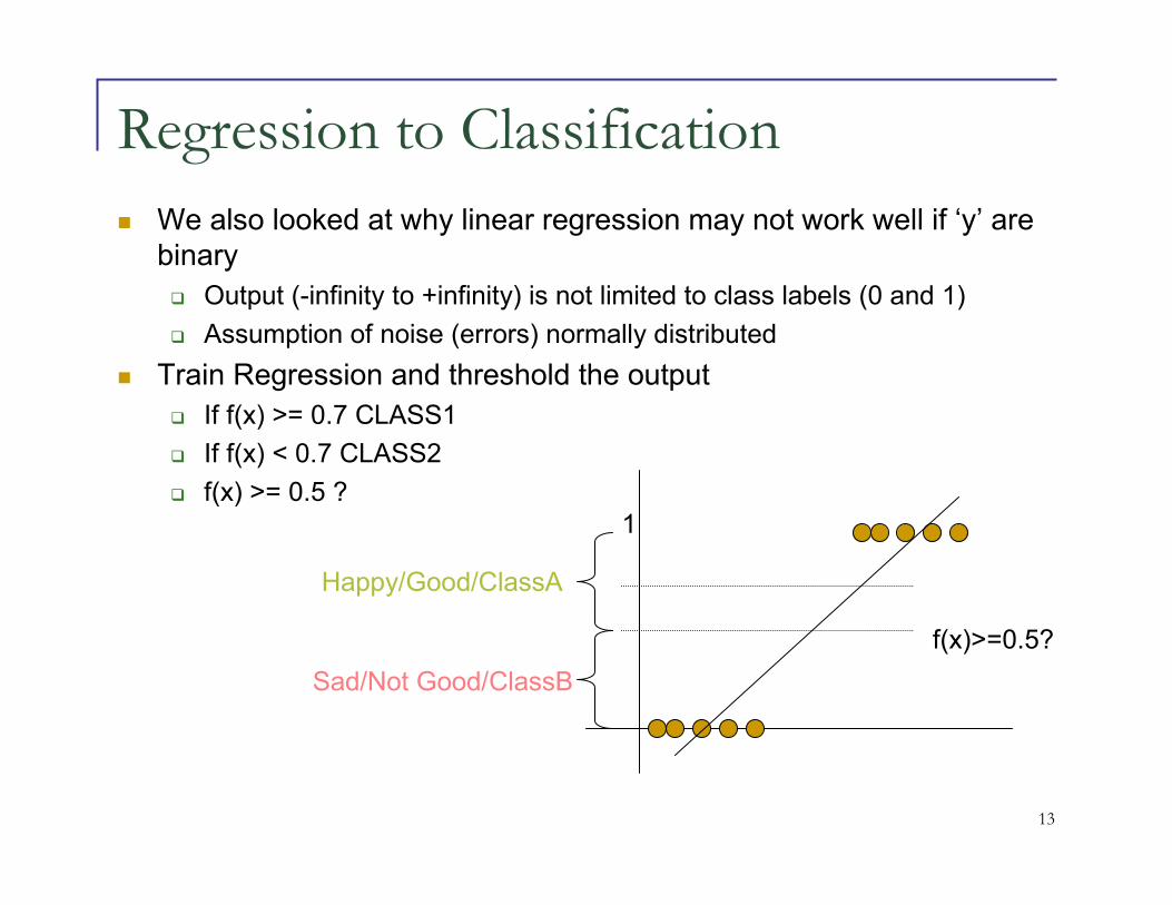
Regression to Classification
� We also looked at why linear regression may not work well if ‘y’ are
binary
� Output (-infinity to +infinity) is not limited to class labels (0 and 1)
� Assumption of noise (errors) normally distributed
� Train Regression and threshold the output
� If f(x) >= 0.7 CLASS1
� If f(x) < 0.7 CLASS2
� f(x) >= 0.5 ?
f(x)>=0.5?
Happy/Good/ClassA
Sad/Not Good/ClassB
1
14
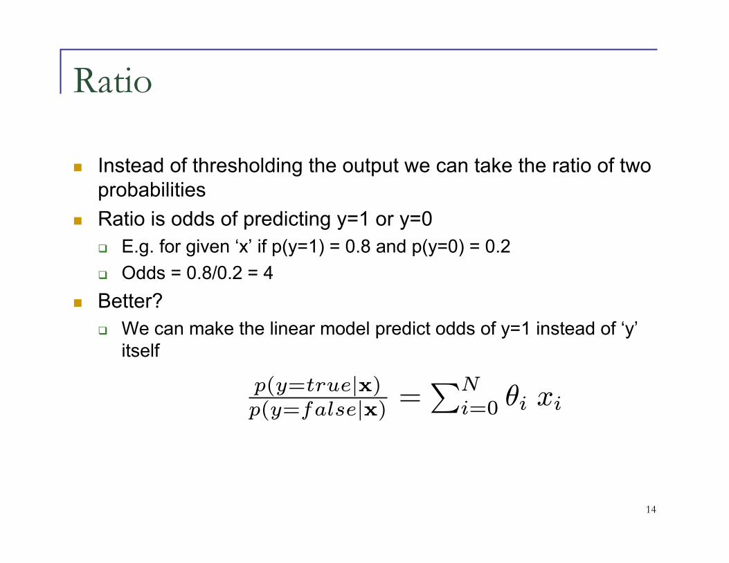
Ratio
� Instead of thresholding the output we can take the ratio of two
probabilities
� Ratio is odds of predicting y=1 or y=0
� E.g. for given ‘x’ if p(y=1) = 0.8 and p(y=0) = 0.2
� Odds = 0.8/0.2 = 4
� Better?
� We can make the linear model predict odds of y=1 instead of ‘y’
itself
p(y=true|x)p(y=false|x)
=∑Ni=0 θi xi

15
Log Ratio
� LHS is between 0 and infinity, we want to be able to handle –
infinity to +infinity which RHS can produce
� If we take log of LHS, it can also range between –infinity and
+ve infinity
log( p(y=true|x)p(y=false|x)
)
log( p(y=true|x)(1−p(y=true|x)
)
p(y=true|x)p(y=false|x)
=∑Ni=0 θi xi
logit(p(x)) = log p(x)1−p(x)

16
Logistic Regression
� Logistic Regression: A Linear Model in which we
predict logit of probability instead of probability
log( p(y=true|x)(1−p(y=true|x)
) =∑Ni=0 θi × xi
log( p(y=true|x)(1−p(y=true|x)
) = w · f
17
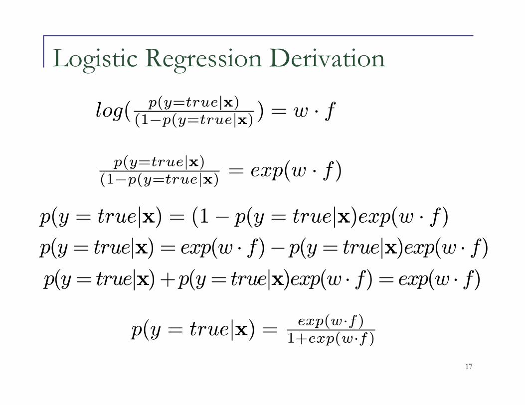
Logistic Regression Derivation
log( p(y=true|x)(1−p(y=true|x)
) = w · f
p(y=true|x)(1−p(y=true|x)
= exp(w · f)
p(y = true|x) = exp(w · f)−p(y = true|x)exp(w · f)
p(y= true|x)+p(y= true|x)exp(w · f) = exp(w · f)
p(y = true|x) = exp(w·f)1+exp(w·f)
p(y = true|x) = (1− p(y = true|x)exp(w · f)
18
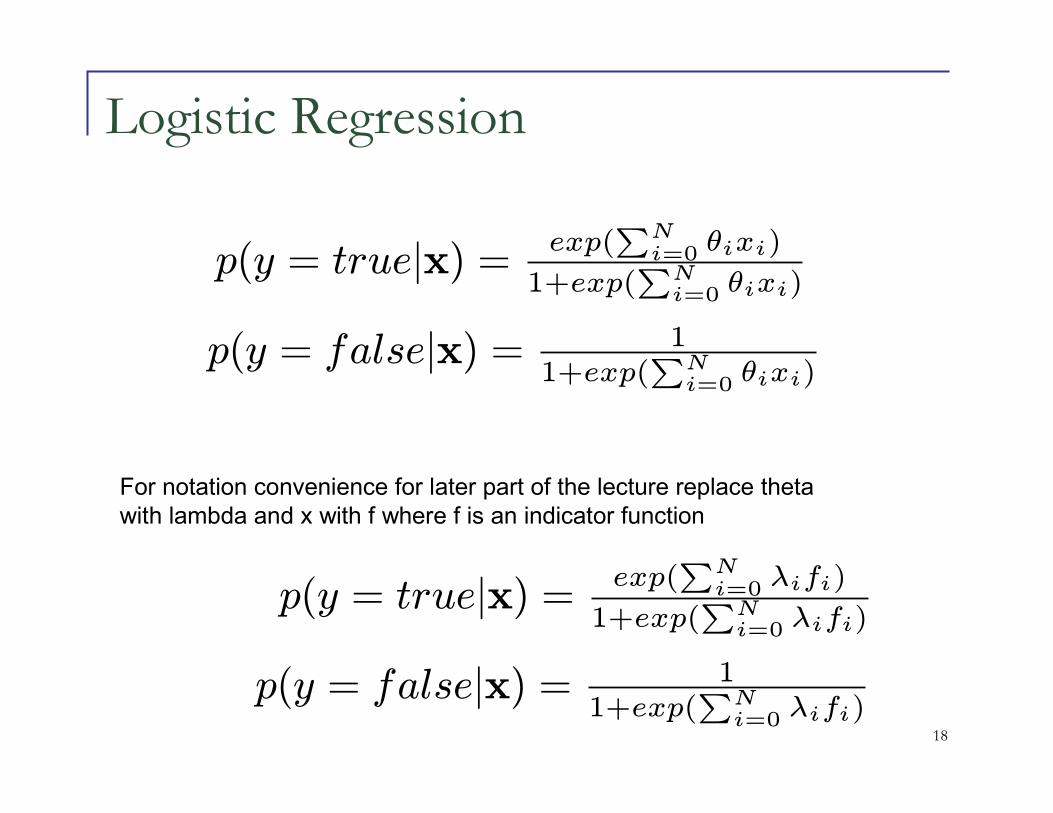
Logistic Regression
p(y = true|x) =exp(
∑Ni=0 θixi)
1+exp(∑
Ni=0 θixi)
p(y = false|x) = 11+exp(
∑Ni=0θixi)
For notation convenience for later part of the lecture replace theta
with lambda and x with f where f is an indicator function
p(y = true|x) =exp(
∑Ni=0 λifi)
1+exp(∑
Ni=0 λifi)
p(y = false|x) = 11+exp(
∑Ni=0λifi)
19
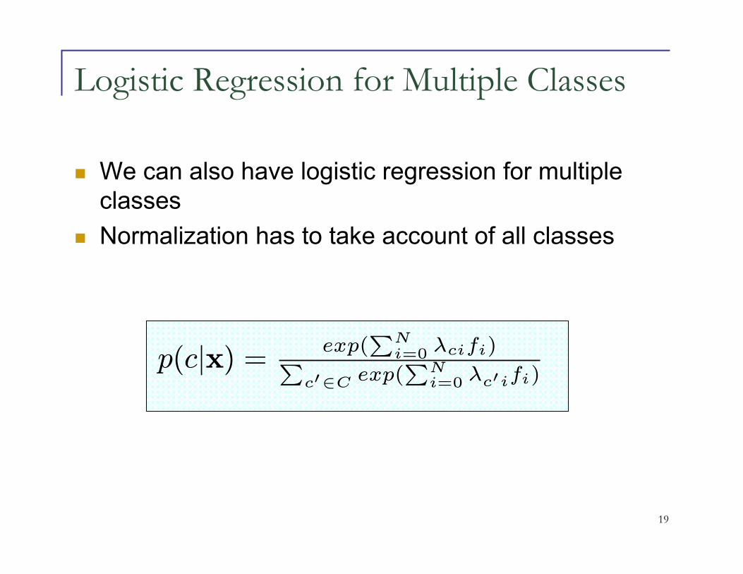
Logistic Regression for Multiple Classes
� We can also have logistic regression for multiple
classes
� Normalization has to take account of all classes
p(c|x) =exp(
∑Ni=0 λcifi)∑
c′∈C exp(∑
Ni=0 λc′ifi)

20
Exponential Models
� Turns out logistic regression is just a type of
exponential model
� Linear combination of weights and features to
produce a probabilistic model
p(c|x) =exp(
∑Ni=0 λcifi)∑
c′∈C exp(∑
Ni=0 λc′ifi)

21
How Can We Estimate Weights
� How to estimate weights (Lambdas)
� For linear regression computed loss function and found
derivative to zero
� We can estimate weights by maximizing (conditional)
likelihood of data according to the model
So why did we talk all about logistic regression when
we were trying to learn Maximum Entropy Models?
Let’s find out

22
Maximum Entropy
� We saw what entropy is
� We want to maximize entropy
� Maximize subject to feature-based constraints
� Feature based constraints help us bring the model distribution close to empirical distribution (data)
� In other words it increases maximum likelihood of data given the model but makes the distribution less uniform
H
Pheads
Fair coin has the highest
entropy
H(p) = −∑x p(x)log2p(x)

23
Constraints on a Entropy Function
Figure below is from Klein, D. and Manning, C., Tutorial [1]

24
Features
� We have seen many different types of features
� Count of words, length of docs, etc
� We can think of features as indicator functions that
represent co-occurrence relation between input
phenomenon and the class we are trying to predict
fi(cd) = φ(d) ∧ cd = ci

25
Example: Features for POS Tagging
� f1(c,d) = { c=NN Λ curword(d)=book Λ
prevword(d)=to}
� f2(c,d) = { c=VB Λ curword(d)=book Λ
prevword(d)=to}
� f3(c,d) = { c=VB Λ curword(d)=book Λ
Λ prevClass(d)=ADJ}

26
Maximum Entropy Example
NN JJ NNS VB
1/4 1/4 1/4 1/4
Add a constraint P(NN) + P(JJ) + P(NNS) = 1
1/3 1/3 1/3 0
Add another constraint P(NN) + P(NNS) = 8/10
4/10 2/10 4/10 0
Given Event space
Maximum Entropy Distribution
27
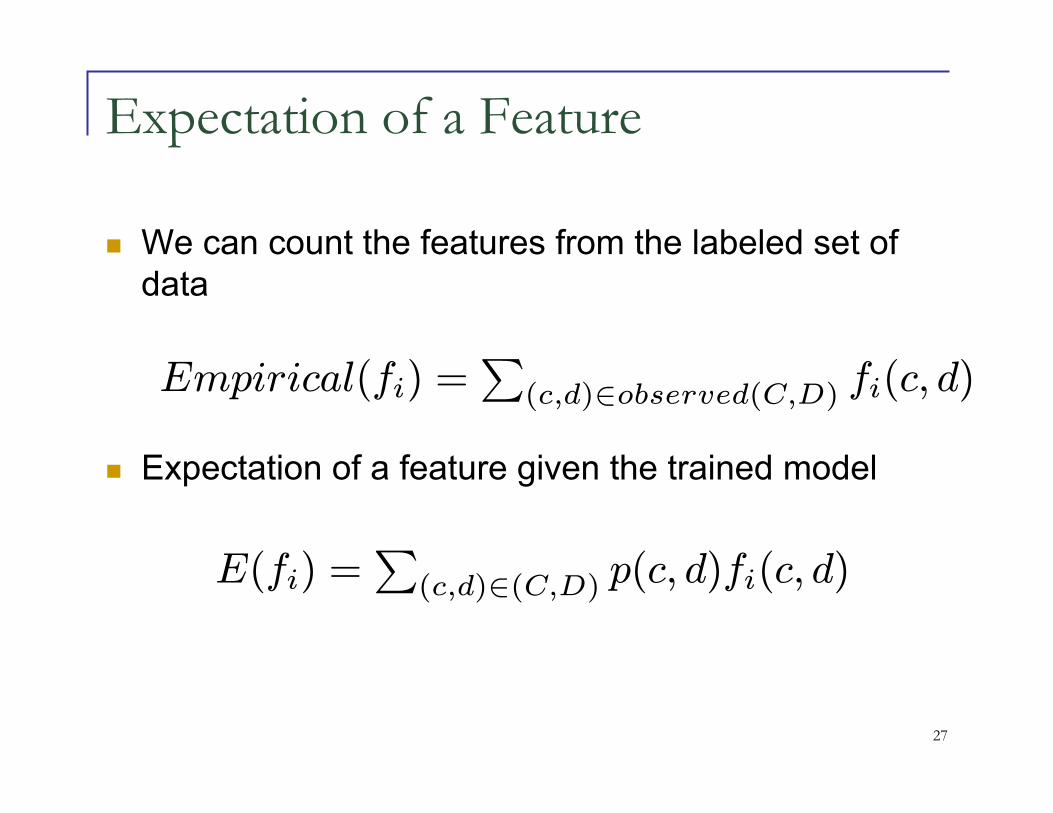
Expectation of a Feature
� We can count the features from the labeled set of
data
� Expectation of a feature given the trained model
Empirical(fi) =∑
(c,d)∈observed(C,D) fi(c, d)
E(fi) =∑
(c,d)∈(C,D) p(c, d)fi(c, d)

28
Maximization with Constraints
maxp(x)H(p) = −∑x p(x)logp(x)
∑x p(x) = 1
s.t.∑x p(x)fi(x) =
∑x˜p(x)fi(x), i = 1...N

29
Solving MaxEnt
� MaxEnt is a convex optimization problem with
concave objective function and linear
constraints
� We have seen such optimization problems
before
� Solved with Lagrange multipliers

30
Lagrange Equation
L(p, λ) = −∑x p(x)logp(x) + λ0[
∑x p(x)− 1]+
∑Ni=1 λi[
∑x p(x)fi(x)−
∑x˜p(x)fi(x)]
Lagrangian gives us unconstrained
optimization as constraints are built into the
equation. We can now solve it by setting
derivatives to zero

31
Maximum Entropy and Logistic Regression
� This unconstrained optimization problem is a dual
problem equivalent to estimating maximum
likelihood of logistic regression model we saw before
Maximizing entropy subject to our constraints
Is equivalent to
Maximum likelihood estimation over exponential family of pλ(x)
32
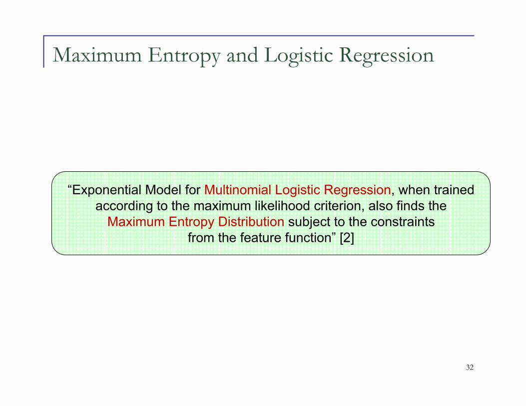
Maximum Entropy and Logistic Regression
“Exponential Model for Multinomial Logistic Regression, when trained
according to the maximum likelihood criterion, also finds the
Maximum Entropy Distribution subject to the constraints
from the feature function” [2]
33
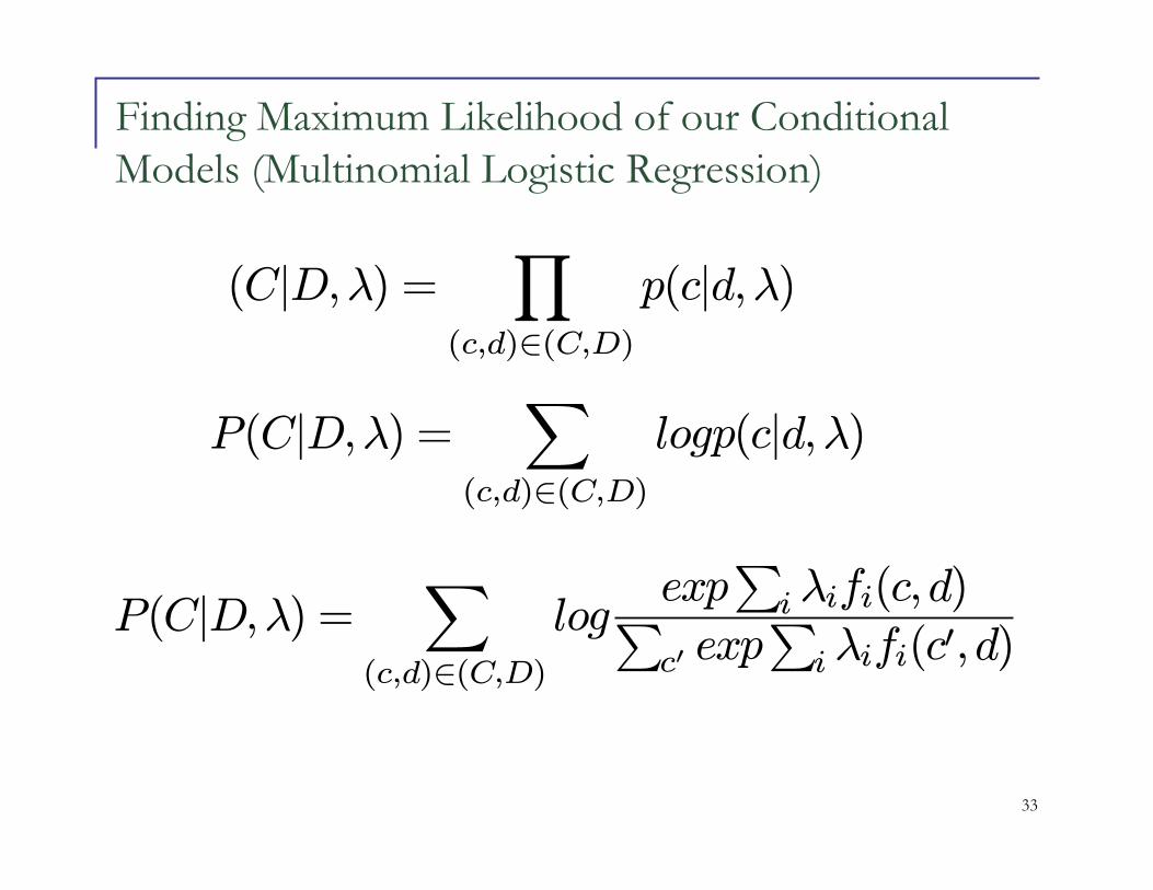
Finding Maximum Likelihood of our Conditional
Models (Multinomial Logistic Regression)
P(C|D,λ) =∑
(c,d)∈(C,D)
logexp
∑i λifi(c,d)∑
c′ exp∑i λifi(c
′, d)
P(C|D,λ) =∑
(c,d)∈(C,D)
logp(c|d,λ)
(C|D,λ) =∏
(c,d)∈(C,D)
p(c|d,λ)

34
Maximizing Conditional Log Likelihood
P(C|D,λ) =∑
(c,d)∈(C,D)
−∑(c,d)∈(C,D) log
∑c′ exp
∑i λifi(c
′, d)
logexp∑iλifi(c,d)
∑
(c,d)∈(C,D)
fi(c, d)−∑
(c,d)∈(C,D)
∑
c′
P (c′|d, λ)fi(c′, d)∂log(P |C,λ)
∂λi=
Empirical count (fi, c) Predicted count (fi, λ)
Optimal parameters are obtained when empirical expectation equal predicted expectation
Taking derivative and setting it to zero

35
Finding Model Parameters� We saw that optimum parameters are obtained when
empirical expectation of a feature equals predicted expectation
� We are finding a model having maximum entropy and satisfying constraints for all features fj
� Hence finding the parameters of maximum entropy model entails to maximizing conditional log-likelihood and solving it� Conjugate Gradient Descent
� Quasi Newton’s Method
� A simple iterative scaling� Features are non-negative (indicator functions are non-negative)
� Add a slack feature
� where
Ep(fj) = E(̃p)(fj)
M = maxi,c∑mj=1 fj(di, c)
fm+1(d, c) =M −∑mj=1 fj(d, c)

36
Generalized Iterative Scaling
� Empirical Expectation
� Initialize m+1 lambdas to 0
� Loop Until Converged
� End loop
Ep̃(fj) =1N
N∑
i=1
fj(di, ci)
Ept(fj) =1N
N∑
i=1
K∑
k=1
P (ck|di)fj(di, ck)
λt+1j = λtj +1Mlog(
Ep̃(fj)Ept (fj)
)

37
Summary
� Logistic Regression
� Maximize conditional log-likelihood to estimate parameters
� Maximum Entropy Model
� Maximize entropy with feature constraints
� Constrained maximization
� Solving for H(p) with maximum entropy is equivalent
to maximizing conditional log-likelihood for our
exponential model

38
References
� [1] Klein, D., Manning C., “Maximum Models,
Conditional Estimation and Optimization” ACL 2003
� [2] Jurafsky, D. and Martin, J., J&M Book, 2nd
Edition
� [3] http://webdocs.cs.ualberta.ca/~swang/me.html