Statistical Mechanics of Soft Core Fluid Mixtures Andrew ... · Statistical Mechanics of Soft Core...
223
Statistical Mechanics of Soft Core Fluid Mixtures Andrew John Archer H. H. Wills Physics Laboratory University of Bristol A thesis submitted to the University of Bristol in accordance with the requirements of the degree of Ph.D. in the Faculty of Science August 2003
Transcript of Statistical Mechanics of Soft Core Fluid Mixtures Andrew ... · Statistical Mechanics of Soft Core...

Statistical Mechanics of
Soft Core Fluid Mixtures
Andrew John Archer
H. H. Wills Physics Laboratory
University of Bristol
A thesis submitted to the University of Bristol in
accordance with the requirements of the degree of
Ph.D. in the Faculty of Science
August 2003


Abstract
In this thesis we investigate the statistical mechanics of binary mixtures of soft-core fluids.
The soft-core pair potentials between the fluid particles are those obtained by considering
the effective potential between polymers in solution. The effective pair potential between
the centers of mass of polymers is well approximated by a repulsive Gaussian potential.
A binary mixture of Gaussian particles can phase separate, and we calculate the phase
diagrams for various size ratios of the two species. Using a simple mean field density
functional theory (DFT) , which generates the random phase approximation for the bulk
pair direct correlation functions, we calculate the surface tension and density profiles for
the free interface between the demixed fluid phases. We find that the asymptotic decay of
the interfacial profiles into bulk can be oscillatory on both sides of the interface. We also
calculate density profiles for the binary Gaussian core model (GCM) adsorbed at a planar
wall and find a wetting transition from partial to complete wetting for certain purely
repulsive wall potentials. By applying a general DFT approach for calculating the force
between two big particles immersed in a solvent of smaller ones we calculate the solvent
mediated (SM) potential between two big Gaussian core particles in the phase separating
binary mixture of smaller GCM particles. We show that the theory for calculating the SM
potential captures effects of thick adsorbed films surrounding the big solute particles and
we find extremely attractive, long ranged SM potentials between the big particles whose
range is determined by the film thickness. In the region of the solvent critical point we
also find extremely attractive SM potentials whose range is now set by the bulk correlation
length in the binary solvent.
In addition to the GCM, we also consider the effective potential between the central
monomers on each polymer chain; this potential features a weak (logarithmic) divergence
as the particle separation r → 0. A binary mixture of these particles can also phase
separate and displays many features in common with the binary GCM.


To my family:
Sarah, Mum, Dad and Alice.


Acknowledgments
First, and foremost, I would like to thank my supervisor, Bob Evans, for all his support,
encouragement and patience, as well as his wisdom in suggesting the topics in this thesis
for me to study. When I started out, I had a suspicion that doing physics could be fun.
Working with Bob has proved to me that my inkling was right: physics is a lot of fun and
to a great extent this has been due to Bob’s enthusiasm.
There are also others I would like to thank: Joe Brader, who answered many of my
questions at the beginning and helped me to get started. Christos Likos and Roland Roth:
great scientists, good collaborators; they are both people I admire and like a lot.
I would also like to acknowledge the Bristol theory group, for providing a good working
atmosphere and for being a friendly group. I mention especially the other PhD students
– my friends and peers: Joe, Ben, Mark, Jorge, Dan, Denzil, Danny, David, Jamie, Maria
and Emma.
Last, but not least, I mention my family: Sarah, my wife, for all her love and support,
and my parents for the same. When, as an 18 year old, I asked my parents what I should
study at university, they encouraged me to do whatever I enjoyed. I have been grateful
for that advice many times.


Authors Declaration
I declare that the work in this thesis was carried out in accordance with the regulations of
the University of Bristol. The work is original except where indicated by special reference
in the text and no part of the thesis has been submitted for any other degree. Any
views expressed in the thesis are those of the author and in no way represent those of
the University of Bristol. The thesis has not been presented to any other University for
examination either in the United Kingdom or overseas.


“...what seems so easy–namely, that the god must be able to make himself
understood–is not so easy if he is not to destroy that which is different.”
Søren Kierkegaard, Philosophical Fragments, edited and translated by
H.V. Hong and E.H Hong, (Princeton, Princeton University Press, 1985).
“He had no beauty or majesty to attract us to him,
nothing in his appearance that we should desire him.”
Isaiah 53:2.


This thesis is based partly on the following papers:
Chapter 5
A.J. Archer and R. Evans,
Binary Gaussian core model: Fluid-fluid phase separation and interfacial properties,
Phys. Rev. E 64 041501 (2001).
Chapter 6
A.J. Archer and R. Evans,
Wetting in the binary Gaussian core model,
J. Phys.: Condens. Matter 14 1131 (2002).
Chapter 7
A.J. Archer, R. Evans and R. Roth,
Microscopic theory of solvent mediated long range forces: Influence of wetting,
Europhys. Lett. 59 526 (2002).
and
A.J. Archer and R. Evans,
Solvent mediated interactions and solvation close to fluid-fluid phase separation: A density
functional treatment,
J. Chem Phys. 118 9726 (2003).
Chapter 8
A.J. Archer, C.N. Likos and R. Evans,
Binary star-polymer solutions: bulk and interfacial properties,
J. Phys.: Condens. Matter 14, 12031 (2002).


Contents
1 Introduction 1
2 Background: Theory of Classical Fluids 5
2.1 Classical fluids . . . . . . . . . . . . . . . . . . . . . . . . . . . . . . . . . . 5
2.2 The Ornstein Zernike equation . . . . . . . . . . . . . . . . . . . . . . . . . 10
2.3 Density functional theory: an introduction . . . . . . . . . . . . . . . . . . . 11
3 A Simple Approach to Inhomogeneous Fluids and Wetting 17
3.1 Landau theory for simple fluids . . . . . . . . . . . . . . . . . . . . . . . . . 18
3.2 Inhomogeneous fluid order parameter profiles . . . . . . . . . . . . . . . . . 20
3.3 Thermodynamics of interfaces . . . . . . . . . . . . . . . . . . . . . . . . . . 22
3.4 Wetting: near to coexistence . . . . . . . . . . . . . . . . . . . . . . . . . . 23
3.5 Landau theory for wetting . . . . . . . . . . . . . . . . . . . . . . . . . . . . 24
3.6 Wetting transitions . . . . . . . . . . . . . . . . . . . . . . . . . . . . . . . . 27
3.7 Incorporating fluctuations . . . . . . . . . . . . . . . . . . . . . . . . . . . . 34
4 The One Component Gaussian Core Model 37
4.1 Introduction: effective interactions . . . . . . . . . . . . . . . . . . . . . . . 37
4.2 A simple model for polymers in solution . . . . . . . . . . . . . . . . . . . . 38
4.3 Properties of the one-component GCM fluid . . . . . . . . . . . . . . . . . . 40
4.4 Solid phases of the GCM . . . . . . . . . . . . . . . . . . . . . . . . . . . . . 43
4.5 DFT theory for the solid phases of the GCM . . . . . . . . . . . . . . . . . 46
5 Binary GCM: Fluid-Fluid Phase Separation and Interfacial Properties 53
5.1 Demixing in binary fluids . . . . . . . . . . . . . . . . . . . . . . . . . . . . 54
5.2 The model mixture and its phase diagram . . . . . . . . . . . . . . . . . . . 56
xv

xvi CONTENTS
5.3 Properties of the fluid-fluid interface . . . . . . . . . . . . . . . . . . . . . . 61
5.3.1 Density profiles . . . . . . . . . . . . . . . . . . . . . . . . . . . . . . 62
5.3.2 Surface tension . . . . . . . . . . . . . . . . . . . . . . . . . . . . . . 66
5.4 Asymptotic decay of correlation functions . . . . . . . . . . . . . . . . . . . 71
5.5 Discussion . . . . . . . . . . . . . . . . . . . . . . . . . . . . . . . . . . . . . 75
6 Wetting in the Binary Gaussian Core Model 79
6.1 Introduction . . . . . . . . . . . . . . . . . . . . . . . . . . . . . . . . . . . . 79
6.2 The model mixture and choice of wall-fluid potentials . . . . . . . . . . . . 80
6.3 Results of calculations . . . . . . . . . . . . . . . . . . . . . . . . . . . . . . 83
6.3.1 First-order wetting transition . . . . . . . . . . . . . . . . . . . . . . 83
6.3.2 Thickness of the wetting film . . . . . . . . . . . . . . . . . . . . . . 86
6.4 Concluding remarks . . . . . . . . . . . . . . . . . . . . . . . . . . . . . . . 89
7 Solvent Mediated Interactions Close to Fluid-Fluid Phase Separation 93
7.1 Introduction . . . . . . . . . . . . . . . . . . . . . . . . . . . . . . . . . . . . 94
7.2 Theory of the solvent mediated potential . . . . . . . . . . . . . . . . . . . 98
7.2.1 General formalism . . . . . . . . . . . . . . . . . . . . . . . . . . . . 98
7.2.2 Application of the RPA functional . . . . . . . . . . . . . . . . . . . 99
7.3 Results for a one-component solvent . . . . . . . . . . . . . . . . . . . . . . 101
7.3.1 Solvent radial distribution function by test-particle route . . . . . . 101
7.3.2 Density profile of small GCM particles around a single big GCM
particle . . . . . . . . . . . . . . . . . . . . . . . . . . . . . . . . . . 102
7.3.3 The SM potential . . . . . . . . . . . . . . . . . . . . . . . . . . . . . 107
7.3.4 The excess chemical potential of the big particle . . . . . . . . . . . 109
7.4 Results for the binary mixture solvent . . . . . . . . . . . . . . . . . . . . . 113
7.4.1 Phase diagram of the binary solvent . . . . . . . . . . . . . . . . . . 113
7.4.2 Density profiles of the binary mixture around a single big GCM
particle . . . . . . . . . . . . . . . . . . . . . . . . . . . . . . . . . . 115
7.4.3 SM potentials for the binary mixture solvent . . . . . . . . . . . . . 120
7.4.4 The excess chemical potential of the big particle immersed in the
binary mixture . . . . . . . . . . . . . . . . . . . . . . . . . . . . . . 123
7.4.5 The SM potential in the vicinity of the binary mixture critical point 126
7.5 Test particle versus OZ route to the SM potential . . . . . . . . . . . . . . . 130
CONTENTS xvii
7.6 Concluding remarks . . . . . . . . . . . . . . . . . . . . . . . . . . . . . . . 133
8 Binary star-polymer solutions: bulk and interfacial properties 143
8.1 Introduction . . . . . . . . . . . . . . . . . . . . . . . . . . . . . . . . . . . . 143
8.2 The model mixture . . . . . . . . . . . . . . . . . . . . . . . . . . . . . . . . 146
8.3 Bulk structure and phase diagram . . . . . . . . . . . . . . . . . . . . . . . 147
8.4 The free fluid-fluid interface . . . . . . . . . . . . . . . . . . . . . . . . . . . 157
8.5 Star-polymers at a hard wall: wetting behaviour . . . . . . . . . . . . . . . 162
8.6 Summary and concluding remarks . . . . . . . . . . . . . . . . . . . . . . . 167
9 Final Remarks 169
A DFT and the Einstein Model 173
B Details of the binary GCM Pole Structure 181
C Derivation of Eq. (7.3.37) for the excess chemical potential 185
D Wetting on Curved Substrates and the Pre-Wetting line 187
E Fourier Transform of the Star Polymer Pair Potential 191
Bibliography 193


List of Figures
2.1 Radial distribution function for a Lennard-Jones fluid . . . . . . . . . . . . 9
3.1 A typical (wetting) density profile for a fluid at a wall . . . . . . . . . . . . 23
3.2 Excess surface grand potential ωex(l), at a continuous wetting transition . . 29
3.3 Excess surface grand potential ωex(l), at a first order wetting transition . . 30
3.4 Equilibrium adsorbed film thickness along paths above, intersecting and
below the pre-wetting line . . . . . . . . . . . . . . . . . . . . . . . . . . . . 32
4.1 The ‘colloid’ approach to polymers in solution . . . . . . . . . . . . . . . . . 39
4.2 g(r) for the GCM at various densities . . . . . . . . . . . . . . . . . . . . . 40
4.3 The HNC g(r) for the GCM near freezing . . . . . . . . . . . . . . . . . . . 42
4.4 Phase diagram for the one component GCM . . . . . . . . . . . . . . . . . . 45
4.5 Helmholtz free energy for an fcc lattice as a function the localization parameter 49
4.6 Phase diagram of the one component GCM . . . . . . . . . . . . . . . . . . 50
5.1 The phase diagram for a mixture of Gaussian particles, equivalent to a
mixture of two polymers with length ratio 2:1 . . . . . . . . . . . . . . . . . 58
5.2 The phase diagram for a mixture of Gaussian particles, equivalent to a
mixture of two polymers with length ratio 3:1 . . . . . . . . . . . . . . . . . 59
5.3 The phase diagram for a mixture of Gaussian particles, equivalent to a
mixture of two polymers with length ratio 5:1 . . . . . . . . . . . . . . . . . 60
5.4 The phase diagram for a mixture of Gaussian particles, equivalent to a
mixture of two polymers with length ratio 1.46:1 . . . . . . . . . . . . . . . 61
5.5 The phase diagram for a symmetric mixture of Gaussian particles . . . . . . 62
5.6 Density profiles at the planar interface . . . . . . . . . . . . . . . . . . . . . 64
5.7 Free interface density profiles for the symmetric GCM fluid . . . . . . . . . 65
xix
xx LIST OF FIGURES
5.8 The surface tension at the planar interface . . . . . . . . . . . . . . . . . . . 67
5.9 The surface tension at the planar interface for the symmetric GCM binary
mixture . . . . . . . . . . . . . . . . . . . . . . . . . . . . . . . . . . . . . . 68
5.10 Plots of the surface segregation and (ω(z) + P ) at the free interface . . . . . 69
5.11 (ω(z) + P ) for the symmetric mixture . . . . . . . . . . . . . . . . . . . . . 70
5.12 The RPA and HNC radial distribution function for the GCM . . . . . . . . 74
6.1 Wetting phase diagram for the binary GCM . . . . . . . . . . . . . . . . . . 82
6.2 Density profiles at a planar wall, for a path in the phase diagram intersecting
the pre-wetting line . . . . . . . . . . . . . . . . . . . . . . . . . . . . . . . . 85
6.3 Density profiles at a planar wall, for a path in the phase diagram below the
pre-wetting line . . . . . . . . . . . . . . . . . . . . . . . . . . . . . . . . . . 86
6.4 The adsorption of species 1 . . . . . . . . . . . . . . . . . . . . . . . . . . . 87
6.5 The pre-factor l0 of the wetting film thickness (l ∼ −l0 ln(x−xcoex.)) versus
the wall potential decay length λ . . . . . . . . . . . . . . . . . . . . . . . . 90
7.1 The density profile of small GCM particles around a single big GCM particle
located at the origin . . . . . . . . . . . . . . . . . . . . . . . . . . . . . . . 105
7.2 The SM potential between two big GCM particles in a pure solvent of small
GCM particles . . . . . . . . . . . . . . . . . . . . . . . . . . . . . . . . . . 108
7.3 Phase diagram for a binary mixture of small GCM particles showing the
thin-thick adsorption transition around a single big GCM particle . . . . . . 114
7.4 The density profiles of a binary solvent of small GCM particles around a
single big GCM test particle, calculated on a path below the thin-thick
adsorbed film transition line . . . . . . . . . . . . . . . . . . . . . . . . . . . 117
7.5 The density profiles of a binary solvent of small GCM particles around a
single big GCM test particle, calculated on a path above the thin-thick
adsorbed film transition line . . . . . . . . . . . . . . . . . . . . . . . . . . . 118
7.6 The density profiles of a binary solvent of small GCM particles around a
single big GCM test particle, calculated on a path intersecting the thin-thick
adsorbed film transition line . . . . . . . . . . . . . . . . . . . . . . . . . . . 119
7.7 The SM potential between two big GCM particles in a binary solvent of
small GCM particles calculated on a path in the phase diagram below the
thin-thick adsorbed film transition line . . . . . . . . . . . . . . . . . . . . . 120

LIST OF FIGURES xxi
7.8 The SM potential between two big GCM particles in a binary solvent of
small GCM particles calculated on a path in the phase diagram intersecting
the thin-thick adsorbed film transition line . . . . . . . . . . . . . . . . . . . 121
7.9 The excess chemical potential of a big GCM particle in a binary solvent of
small GCM particles . . . . . . . . . . . . . . . . . . . . . . . . . . . . . . . 124
7.10 density profiles of a binary mixture of small GCM particles around a big
GCM test particle calculated on a path in the phase diagram approaching
the bulk critical point . . . . . . . . . . . . . . . . . . . . . . . . . . . . . . 128
7.11 SM potential between two big GCM particles in a binary solvent of small
GCM particles, calculated on a path in the phase diagram approaching the
bulk critical point . . . . . . . . . . . . . . . . . . . . . . . . . . . . . . . . . 129
7.12 SM potentials calculated using gbb(r) obtained from the RPA closure to the
OZ equations . . . . . . . . . . . . . . . . . . . . . . . . . . . . . . . . . . . 132
7.13 The pair correlation functions calculated by the test particle route for a
ternary mixture of GCM particles . . . . . . . . . . . . . . . . . . . . . . . . 134
8.1 The partial structure factors, calculated along two different thermodynamic
paths in the (x, ρ)-plane of the star polymer mixture obtained from the HNC
and RPA . . . . . . . . . . . . . . . . . . . . . . . . . . . . . . . . . . . . . 149
8.2 The HNC radial distribution functions gii(r) of the minority phases at high
total densities . . . . . . . . . . . . . . . . . . . . . . . . . . . . . . . . . . . 151
8.3 The RPA-spinodal and binodal lines for the star-polymer mixture along
with the HNC-binodal . . . . . . . . . . . . . . . . . . . . . . . . . . . . . . 153
8.4 Comparison of the HNC- and RPA-results for the partial chemical potentials156
8.5 The fluid-fluid interface density profiles . . . . . . . . . . . . . . . . . . . . 159
8.6 The surface tension at the planar free interface . . . . . . . . . . . . . . . . 161
8.7 Density profiles of a binary star-polymer fluid adsorbed at a wall . . . . . . 163
8.8 Binary star-polymer phase diagram showing the location of the pre-wetting
line . . . . . . . . . . . . . . . . . . . . . . . . . . . . . . . . . . . . . . . . . 164
8.9 Adsorption of species 1 at planar wall, for paths in the phase diagram near
and intersecting the pre-wetting line . . . . . . . . . . . . . . . . . . . . . . 166
8.10 Adsorption of species 1 at planar wall, for paths in the phase diagram below
the pre-wetting line . . . . . . . . . . . . . . . . . . . . . . . . . . . . . . . . 167

xxii LIST OF FIGURES
B.1 Imaginary part of the poles . . . . . . . . . . . . . . . . . . . . . . . . . . . 182
B.2 Real part of the poles . . . . . . . . . . . . . . . . . . . . . . . . . . . . . . 183
D.1 Binary GCM density profiles on a curved substrate . . . . . . . . . . . . . . 188
D.2 Pre-wetting line on a curved substrate . . . . . . . . . . . . . . . . . . . . . 189

Chapter 1
Introduction
“We all agree that your theory is crazy, but is it crazy enough?”
Niels Bohr
The subject of the theory of classical fluids is now well-established. The bulk structure
and thermodynamics of simple (atomic) fluids is reasonably well understood [1], and can
usually be described theoretically with the machinery of integral equations or perturbation
theory. However, the complexity of liquid state problems increases hugely when one is
interested in inhomogeneous fluids, i.e. the fluid in the presence of confining potentials
or at interfaces. These types of problems can often be tackled within density functional
theory (DFT) or simulation, but there is still much to understand, particularly when
there are phenomena such as wetting, associated with phase separation, or bulk criticality
involved.
Some of the focus in the field of liquid-state physics has shifted recently towards com-
plex, colloidal fluids, and this too is the subject of the present thesis. The philosophy of
our approach is to develop simple models for complex soft matter systems that capture
the essential physics. These models then become interesting in their own right, from a
statistical mechanics viewpoint, and often exhibit surprisingly rich features which do not
have direct counterparts for simple (atomic) fluids. One then asks, in turn, whether what
emerges from the models is relevant for real complex fluids. Since it is often possible to
‘tune’ the interactions in complex fluids, for example by the addition of non-adsorbing
polymers or ions to a suspension of colloidal particles, the features emerging from the
simple models are indeed often relevant for real complex fluids.
1

2 Introduction
The particular focus of this thesis concerns simple models of binary polymer solutions
where the interactions between the individual polymer chains are treated using an effective
pair potential between the centers of mass, i.e. a Gaussian pair potential. Sometimes we
consider the effective potential between the central monomers of each polymer (chapter
8). The results from the latter model also pertain to star-polymer solutions. These model
fluids display many novel features arising from the soft (penetrable) cores of the particles.
For example, mean-field theories become increasingly accurate as the density increases.
We have used DFT to calculate various properties for bulk and inhomogeneous binary
mixtures of these model fluids. The binary mixture separates into two phases if the
solution is sufficiently concentrated. Using DFT we have calculated the surface tension
and density profiles of the two species at the interface between the two demixed fluid
phases. The decay of the one-body density profiles at this fluid-fluid interface can be
either monotonic or damped oscillatory; the type of decay is determined by the location of
the state point in the phase diagram relative to the the Fisher-Widom line [2]. The system
is of particular interest since, unlike the liquid-gas interface in simple fluids, pronounced
oscillations in the one-body density profiles can occur on both sides of the interface.
We calculated the density profiles of the binary Gaussian fluid at purely repulsive
planar walls and found that for state points close to phase separation, complete wetting
films of the coexisting fluid phase can develop at the wall – see Ch. 6. In addition we
found that there is a wetting transition – i.e. for some state points at bulk coexistence
the thickness of the fluid film adsorbed at the wall is finite, but as the total fluid density
is decreased, staying at coexistence, there is a transition to a macroscopic thick adsorbed
film. This transition can be first or second order, depending on the form of the wall po-
tential, however, in this thesis we focus on the first-order transition regime. We use a fully
microscopic fluid theory, the results from which can be used to test other mesoscopic (ef-
fective interfacial Hamiltonian) descriptions of the wetting transition. Our results support
the general scheme of using effective interfacial Hamiltonians. We have also examined the
phenomenology for a different model fluid: the central-monomer (star-polymer) effective
potential.
A separate aspect of the work with Gaussian particles was to use the same simple
model to implement a general DFT method for calculating solvent mediated (SM) poten-
tials. This is a powerful way of treating multi-component fluids. One is attempting to
determine an effective interaction potential between particles of one species in a solution of

Introduction 3
another or several, generally smaller, species of particles. Much of the motivation for cal-
culating effective SM potentials in complex (multi-component) fluids is that a theoretical
treatment of the full mixture is often prohibitively difficult, particularly when there is a
big size asymmetry between the different species of particles in the fluid. This difficulty is
especially pronounced when one is interested in inhomogeneous systems. Formally the aim
is to integrate out the degrees of freedom of the small particles in the system, describing
their effect by means of an effective solvent (small particle) mediated potential between
the big particles. Roth, Evans and collaborators [3, 4] introduced a general DFT scheme
within which one can calculate solvent mediated potentials. This proved very effective for
hard sphere fluids where the solvent mediated potential is termed the depletion potential.
What is of particular interest is whether this (mean-field) theory can include effects such as
a wetting film of the small particles around the big particle, or critical fluctuations in the
small particle solvent fluid. Moreover these effects can result in long ranged SM potentials,
which are important when considering segregation and the stability of multi-component
fluid mixtures. When these long ranged SM potentials are attractive they can provide a
mechanism for flocculation in colloidal suspensions. These effective SM potentials can be
measured directly in colloidal systems by trapping a pair of colloids close together with
optical tweezers, and using video-microscopy to obtain the SM potential from the averaged
motion of the colloids in the traps – see for example Ref. [5]. Using the mean-field DFT
for the Gaussian core model fluid of polymers in solution, we were able to include the
effects of thick (wetting) films of the small solvent particles around the big particles and
take account of critical solvent fluctuations, in determining the SM potential between the
large particles. Because of the simplicity of the model Gaussian fluid we were able to find
an analytic approximation to the SM potential in some particular cases, thereby gaining
much insight into the general method.
This thesis proceeds as follows: In chapters 2 and 3 we provide the background theory
that the rest of the thesis is built upon. Ch. 2 is a general introduction to liquid state
theory, with a particular focus on DFT. In Ch. 3 we demonstrate (within Landau theory)
some of the phenomenology of inhomogeneous fluids, with a strong emphasis on wetting
and wetting transitions. In Ch. 4 we introduce the Gaussian core model – both the fluid
and solid phases. In Ch. 5 we introduce the binary Gaussian core model, which can
phase separates into two fluid phases at sufficiently high densities, and in this chapter
we calculate phase diagrams and various properties of the interface between the demixed

4 Introduction
phases, including interfacial density profiles and the surface tension. In Ch. 6 we calculate
the density profiles for the binary Gaussian fluid at a planar wall, where we find a wetting
transition from partial to complete wetting for certain purely repulsive wall potentials. Ch.
7 is where we determine the SM potential between two big Gaussian particles, immersed in
a binary solvent of smaller Gaussian particles. In Ch. 8 we consider the central-monomer
effective pair potential model for a binary polymer solution and show that this exhibits
features very similar to those described in Chs. 5 and 6 for the binary Gaussian core model.
In Ch. 9 we make a few final remarks.

Chapter 2
Background:
Theory of Classical Fluids
In this chapter we briefly introduce the theory of classical fluids, composed of spherically
symmetric particles. We will describe some methods for calculating bulk thermodynamic
quantities and correlation functions and subsequently provide a brief introduction to density
functional theory, a formalism within which one can calculate properties of inhomogeneous
fluids. This theory focuses on calculating the fluid density profile in the presence of an
external potential such as a confining wall.
2.1 Classical fluids
Classical fluids are those where the quantum mechanical nature of the underlying sub-
atomic particle interactions can be neglected and the interactions between the fluid parti-
cles can be treated in a purely classical way. This approximation is a good one for atomic
fluids if the atoms are sufficiently massive and the temperature is sufficiently high. For
example, liquid argon can be treated as a classical fluid with great success, whereas liquid
helium cannot. A good indicator for when quantum mechanical effects can be neglected
is if the thermal de Broglie wavelength Λ ¿ d, where
Λ =
√
2πβ~2
m. (2.1.1)
β = 1/kBT is the inverse temperature, m is the mass of the atom and d is the average
separation between the atoms, which in a liquid is normally of order the diameter of the
5

6 Background: Theory of Classical Fluids
atoms. Colloidal fluids are also well described within a classical treatment.
The following discussion of classical fluids largely follows the standard presentation of
the subject, e.g. Hansen and McDonald [1]. The starting point for the theory is defining
the effective interaction potential between the particles in the fluid, Φ(rN ), where rN =
r1, r2, ...rN denotes the set of position coordinates for the N particles in the system.
The effective potential between the particles includes all the underlying interactions such
as the Coulomb forces between the electrons and ions of the atoms. The Hamiltonian for
such a system is
H(pN , rN ; N) =N
∑
i=1
p2i
2m+ Φ(rN ) +
N∑
i=1
V (ri), (2.1.2)
where pi denotes the momentum of and V (ri) the one-body external potential acting on
the ith particle. A further approximation often made is the assumption that the effective
potential between the particles is pairwise additive, i.e.
Φ(rN ) =1
2
∑
j 6=i
N∑
i=1
v(|ri − rj |), (2.1.3)
where v(r) is the potential between a pair of particles separated by a distance r. An
example of such an effective pair potential is the Lennard-Jones potential which provides
a good approximation for the effective potential between the atoms in a simple fluid such
as liquid argon [1]. The Lennard-Jones potential is
v(r) = 4ε
(
(σLJ
r
)12−
(σLJ
r
)6)
, (2.1.4)
where σLJ is roughly the atomic diameter and ε is a parameter which measures the strength
of the attractive part of the potential. The r−12 term models the repulsive core, which
arises from the Pauli repulsion between the atomic electrons and the attractive r−6 term
arises from the induced dipole-induced dipole interaction between the atoms at larger
separations.
Having specified the form of the interactions between the particles, the Hamiltonian
is fully determined and equilibrium thermodynamic quantities and correlation functions
can, in principle, be calculated. The equilibrium value of a phase function O(pN , rN ; N)
in the Grand canonical ensemble is given by
〈O〉 =∞
∑
N=0
∫
drN
∫
dpNO(pN , rN ; N)f(pN , rN ; N), (2.1.5)

2.1 Classical fluids 7
where f(pN , rN ; N) is the probability density for a given configuration of the system
coordinates (pN , rN ) and we denote the product dr1dr2...drN by drN . For example, the
internal energy is
U =
∞∑
N=0
∫
drN
∫
dpNH(pN , rN ; N)f(pN , rN ; N). (2.1.6)
The idea behind this approach, due to Gibbs, is that the equilibrium state of the system can
be determined by considering an ensemble of identical systems. By summing (integrating)
over the probabilities of each of the different configurations that occur, one can determine
equilibrium quantities. The form of f depends upon which ensemble of systems one is
considering. In the Grand canonical ensemble one fixes the volume V , temperature T
and chemical potential µ of the system. One can consider other ensembles, but in the
thermodynamic limit, V, N → ∞, they are all equivalent. In the Grand canonical ensemble
f(pN , rN ; N) =h−3N
N !
exp[βNµ − βH(pN , rN ; N)]
Ξ(µ, V, T ), (2.1.7)
where the Grand partition function Ξ(µ, V, T ) is
Ξ(µ, V, T ) =∞
∑
N=0
h−3N
N !
∫
drN
∫
dpN exp[βNµ − βH(pN , rN )]
= Trcl exp[βNµ − βH(pN , rN ; N)]. (2.1.8)
We have used Trcl to denote the classical trace in Eq. (2.1.8). The partition function is a
key quantity in statistical mechanics, and it forms a link to thermodynamics because the
grand potential of the system is simply
Ω = −kBT ln Ξ. (2.1.9)
The integral in Eq. (2.1.8) over the momentum degrees of freedom is straightforward,
so the partition function can be expressed as just an integral over the configurational
(position) degrees of freedom:
Ξ =∞
∑
N=0
zN
N !
∫
drN exp[−βΦ(rN ) − βN
∑
i=1
V (ri)], (2.1.10)
where the activity z = Λ−3 exp(βµ). Starting from Eq. (2.1.10), if we only perform a
partial trace over the configurational degrees of freedom, we can generate a hierarchy of
particle distribution functions:
ρ(n)(rn) =1
Ξ
∞∑
N≥n
zN
(N − n)!
∫
dr(N−n) exp[−βΦ(rN ) − βN
∑
i=1
V (ri)]. (2.1.11)

8 Background: Theory of Classical Fluids
If we consider the homogeneous situation, where the external potential V (ri) = 0, then
the first member of the hierarchy, ρ(1)(r) is then simply the one-body density of the fluid,
which is a constant:
ρ(1)(r) =〈N〉V
= ρ. (2.1.12)
We will now focus on the second member of the hierarchy, the two-body distribution
function ρ(2)(r1, r2). This is proportional to the probability of finding another particle
at r2, given there is already a particle at r1. For a fluid of spherically symmetric par-
ticles in the bulk, where the external potential is zero, translational invariance demands
ρ(2)(r1, r2) = ρ(2)(|r1−r2|) = ρ(2)(r12). It is also useful to introduce the radial distribution
function, g(r) = ρ(2)(r)/ρ2. When the particles in the fluid are far apart, r → ∞, then
their positions are uncorrelated, and g(r) → 1. However, in a dense fluid, when the sepa-
ration between the particles is only a few particle diameters, g(r) can be highly structured.
A typical plot of g(r) for a dense liquid well away from the critical point is plotted in Fig.
2.1. This was calculated using the Percus-Yevick closure to the Ornstein-Zernike equation
(details in the next section) for a fluid of particles which interact via the Lennard-Jones
potential, Eq. (2.1.4), at a temperature kBT/ε = 2.0 and density ρσ3LJ = 0.8. In a dense
fluid, when r is only a few σLJ , g(r) can be highly oscillatory due to the packing of the
hard cores of the particles.
There are several reasons for focusing on the radial distribution function. Firstly, the
Fourier transform of the radial distribution function, the fluid structure factor, S(k), is
a quantity that is directly accessible in diffraction experiments (normally neutron or x-
ray scattering, although if the particles are larger (colloids), then one can also use light
scattering). The liquid structure factor is given by
S(k) = 1 + ρ
∫
dr (g(r) − 1) exp(ik.r). (2.1.13)
Another reason for focusing on the radial distribution function is that once it is known,
one can use it to calculate thermodynamic quantities. For example, the k → 0 limit of
S(k) is related to the isothermal compressibility χT by the compressibility equation
χT ≡ 1
ρ
(
∂ρ
∂P
)
T
=S(0)
ρkBT. (2.1.14)
For a system in which particles interact solely via a pairwise potential, v(r), (see Eq.
(2.1.3)), the internal energy of the system, Eq. (2.1.6), can be simplified to yield the

2.1 Classical fluids 9
0 1 2 3 4 5r/σLJ
0
0.5
1
1.5
2
2.5
g(r)
Figure 2.1: The radial distribution function for a Lennard-Jones fluid, at a reduced tem-
perature kBT/ε = 2.0 and fluid density ρσ3LJ = 0.8, calculated using the Percus-Yevick
closure to the Ornstein-Zernike equation.
internal energy per particle in terms of an integral involving only g(r):
U
N=
3
2kBT +
ρ
2
∫
dr g(r)v(r). (2.1.15)
This is known as the energy equation. Similarly, one can derive an equation for the
pressure, known as the virial equation [1]:
P = ρkBT − ρ2
6
∫
dr g(r)rdv(r)
dr. (2.1.16)
The radial distribution function for a particular model fluid can be determined in several
ways. One way is to perform a computer simulation of the fluid. This could either be
done by solving Newton’s equations, a molecular dynamics simulation, or by generating
random fluid configurations and calculating the Boltzmann weight for each configuration –
this is a Monte Carlo simulation. Another approach is that based on perturbation theories.
Here the idea is to split the pair potential of the fluid into two parts, the reference part
(normally the harshly repulsive core part) and the perturbation. The correlations in the
fluid due to the core part can be modeled by, for example, those of a hard sphere potential.
There is much known about this system and the hard-sphere radial distribution function is
well-known. One then calculates the full g(r) by perturbing about the hard-sphere result

10 Background: Theory of Classical Fluids
[1]. Another approach, which is the basis of many successful theories for g(r) in a bulk
fluid, is that based on closure approximations to the Ornstein-Zernike equation.
2.2 The Ornstein Zernike equation
In bulk, the radial distribution function for an ideal gas, g(r) = 1 for all values of r,
i.e. there are no correlations between the particles. For a real fluid, one can define a
total correlation function, h(r), as the deviation of g(r) from the ideal gas result, i.e.
h(r) = g(r)−1. The Ornstein Zernike (OZ) approach to calculating h(r) is to split up the
correlations present in h(r) into a ‘direct’ part, which will include the correlations over a
range of order the range of the pair potential, and an ‘indirect’ part, i.e. the rest. This
idea is the basis of the OZ integral equation:
h(r) = c(2)(r) + ρ
∫
dr′c(2)(|r − r′|)h(r′), (2.2.1)
where c(2)(r) is the direct pair correlation function, which is generally less structured than
h(r) and has the range of the pair potential. Eq. (2.2.1) as it stands does not enable us
to calculate h(r); we have merely shifted the problem from calculating h(r) to calculating
c(2)(r). Eq. (2.2.1) can be viewed as an equation defining c(2)(r). In order to solve Eq.
(2.2.1) we also need a closure relation, an additional equation relating c(2)(r) to h(r),
which we can use with the OZ equation, Eq. (2.2.1), to solve for h(r). The exact closure
equation can generally not be determined, and so one is forced to resort to making an
approximation. The usual route is to make a diagrammatic expansion for the correlation
functions and truncate the (infinite) series at some point or perform a re-summation [1].
For example, the Percus-Yevick closure relation [1], which was used to calculate g(r) in
Fig. 2.1, is
c(2)PY (r) = (1 − exp[βv(r)])(1 + h(r)). (2.2.2)
This closure is particularly good for fluids with short ranged potentials and sharply repul-
sive cores. Another closure relation is the hypernetted chain (HNC), given by [1]
c(2)HNC(r) = −βv(r) + h(r) − ln(1 + h(r)). (2.2.3)
This closure turns out to be particularly good for soft-core, purely repulsive pair potentials,
such as the Coulomb potential (the one component classical plasma consisting of point
particles in a neutralizing background), and in particular the Gaussian core model (GCM),

2.3 Density functional theory: an introduction 11
where the particles interact via a repulsive Gaussian potential. These particles are the
subject of this thesis. What is even more striking is that for the GCM, when the fluid
density is high, then a particularly simple closure, the random phase approximation (RPA),
is also reasonably accurate:
c(2)RPA(r) = −βv(r), for all r. (2.2.4)
We shall return to this subject in the next section where we will describe how the OZ
equation arises naturally in the context of density functional theory.
2.3 Density functional theory: an introduction
The discussion in this section is drawn mainly from the articles by Evans [6, 7]. The
focus of density functional theory (DFT) is the one body density profile, ρ(1)(r), the first
member of the hierarchy of particle distribution functions, defined by Eq. (2.1.11). DFT is
therefore a theory for inhomogeneous fluids. If we introduce the particle density operator
ρ(r) =N
∑
i=1
δ(r − ri), (2.3.1)
then we can express the partition function, Eq. (2.1.10), in terms of the particle density
operator:
Ξ =∞
∑
N=0
Λ−3N
N !
∫
drN exp[−βΦ(rN ) + β
∫
drρ(r)u(r)], (2.3.2)
where u(r) = µ − V (r). The logarithm of the partition function is the Grand potential
Ω (see Eq. (2.1.9)), and so the functional derivative of Ω with respect to u(r) is simply
−〈ρ(r)〉, which is the first member of the hierarchy of particle distribution functions, Eq.
(2.1.11):δΩ
δu(r)= −〈ρ(r)〉 = −ρ(1)(r). (2.3.3)
A second derivative yields the density-density correlation function
β−1 δ2Ω
δu(r2)δu(r1)= G(r1, r2) = 〈ρ(r1)ρ(r2)〉 − ρ(1)(r1)ρ
(1)(r2), (2.3.4)
from which we can obtain the second member of the hierarchy of particle distribution
functions ρ(2)(r1, r2) (see Eq. (2.1.11)), since
ρ(2)(r1, r2) = 〈ρ(r1)ρ(r2)〉 − 〈ρ(r1)〉 δ(r1 − r2). (2.3.5)

12 Background: Theory of Classical Fluids
Further differentiation yields the higher order particle distribution functions. It should
be emphasized that Eq. (2.3.3) is exact and does not just apply to fluids interacting
via pairwise additive potentials Eq. (2.1.3). The one body density, which we will now
denote ρ(r), is therefore a functional of u(r). It can be shown that, for a given Φ(rN ),
µ and β, ρ(r) is uniquely determined by the external potential V (r) [6, 8]. Similarly the
equilibrium probability density f (see Eq. (2.1.7)) is also a functional of the density ρ(r).
We can therefore construct a quantity
F [ρ] = Trcl[f(H −∫
drρ(r)V (r) + β−1 ln f)], (2.3.6)
which is a unique functional of the one-body density [6, 7]. From this functional is con-
structed a second functional:
ΩV [ρ′] = F [ρ′] −∫
drρ′(r)[µ − V (r)]. (2.3.7)
When the density in Eq. (2.3.7), ρ′(r), is the equilibrium density profile, ρ(r), then ΩV [ρ]
is equal to the grand potential Ω [6] and the total Helmholtz free energy is
F = F [ρ] +
∫
drρ(r)V (r), (2.3.8)
and we identify F [ρ] as the intrinsic Helmholtz free energy. The fact that the equilibrium
density profile ρ(r) minimizes the functional ΩV [ρ] results in the following variational
principle:
δΩV [ρ′]
δρ′(r)
∣
∣
∣
∣
∣
ρ′=ρ
= 0 (2.3.9)
and
ΩV [ρ] = Ω. (2.3.10)
Inserting Eq. (2.3.7) into Eq. (2.3.9) yields:
µ = V (r) +δF [ρ]
δρ(r). (2.3.11)
If the fluid is at equilibrium, then the chemical potential µ is a constant throughout the
inhomogeneous fluid and the term δF [ρ]/δρ(r) in Eq. (2.3.11) is the intrinsic contribution
to the chemical potential.
When the fluid is an ideal gas, then the intrinsic Helmholtz free energy functional is
simply
Fid[ρ] = β−1
∫
drρ(r) [ln Λ3ρ(r) − 1]. (2.3.12)

2.3 Density functional theory: an introduction 13
For a real fluid we can then divide the intrinsic Helmholtz free energy into an ideal gas
part, Eq. (2.3.12), and an excess part, which takes into account the correlations between
the particles in the fluid, i.e. F [ρ] = Fid[ρ] + Fex[ρ]. Eq. (2.3.11) therefore becomes
Λ3ρ(r) = exp[βu(r) + c(1)(r)] (2.3.13)
where we have used δFid/δρ(r) = β−1 ln Λ3ρ(r), the ideal gas contribution to the intrinsic
chemical potential and c(1)(r) is the excess (over ideal) term:
c(1)(r) ≡ −βδFex[ρ]
δρ(r). (2.3.14)
c(1)(r) is the one-body direct correlation function and is itself a functional of ρ(r). Fur-
ther differentiation with respect to the density generates the direct correlation function
hierarchy [6, 7]:
c(n)(rn) =δc(n−1)(rn−1)
δρ(rn). (2.3.15)
Of particular interest is the two-body direct correlation function:
c(2)(r1, r2) =δc(1)(r1)
δρ(r2)= −β
δ2Fex[ρ]
δρ(r2)δρ(r1). (2.3.16)
We have thus identified the direct pair correlation function, c(2)(r1, r2), for an inhomoge-
neous fluid. We introduced this function in the context of the OZ equation, Eq. (2.2.1),
for homogeneous fluids in the previous section. This identification is proved as follows: If
we insert Eq. (2.3.13) into Eq. (2.3.16), we find
c(2)(r1, r2) =δ(r1 − r2)
ρ(r1)− β
δu(r1)
δρ(r2)(2.3.17)
The second term on the right hand side of Eq. (2.3.17) is the functional inverse, G−1(r1, r2),
of the density-density correlation function (see Eq. (2.3.4)). A functional inverse is defined
by∫
dr3 G−1(r1, r3)G(r3, r2) = δ(r1 − r2). (2.3.18)
Substituting Eqs. (2.3.4), (2.3.5) and (2.3.17) into Eq. (2.3.18) and defining the inhomo-
geneous fluid total correlation function h(r1, r2) by ρ(r1)ρ(r2)h(r1, r2) = ρ(2)(r1, r2) −ρ(r1)ρ(r2), we obtain the OZ equation for an inhomogeneous fluid [6, 7]:
h(r1, r2) = c(2)(r1, r2) +
∫
dr3 h(r1, r3)ρ(r3)c(2)(r3, r2). (2.3.19)
14 Background: Theory of Classical Fluids
When the fluid density is a constant, ρ(r) = ρ, then this reduces to Eq. (2.2.1), the
homogeneous fluid OZ equation.
As was the case for the homogeneous OZ equation, there are very few model fluids
for which the inhomogeneous direct pair correlation function, c(2)(r1, r2), is known. How-
ever, DFT provides a formalism within which controlled approximations can be made
for c(2)(r1, r2) and hence for c(1)(r). These approximations, together with Eq. (2.3.13),
provide a prescription for calculating the inhomogeneous fluid density profile, ρ(r). Such
approximations are generally mean field in nature and so these DFT theories exhibit the
mean field critical exponents for diverging quantities, such as the bulk correlation length,
near the bulk critical point. They will also generate mean-field exponents for diverging
interfacial thermodynamic quantities and correlation lengths – see Ch. 3. One route used
to generate approximations for Fex, is to start from a functional integration of Eq. (2.3.16)
[6, 7] and then focus on making an approximation for c(2)(r1, r2). An alternative route
for determining Fex (a route limited to fluids where the potential function is pairwise
additive – i.e. Eq. (2.1.3) holds) is as follows: One can recast the potential energy term in
the Hamiltonian, Eq. (2.1.3), as [7]:
Φ(rN ) =1
2
∫
dr1
∫
dr2v(|r1 − r2|)ρ(r1)(ρ(r2) − δ(r1 − r2)). (2.3.20)
Inserting this expression into the partition function, Eq. (2.3.2), we find that on differen-
tiating the partition function with respect to the pair potential v(r1, r2) we arrive at the
following equation:
δΩ
δv(r1, r2)=
1
2(〈ρ(r1)ρ(r2)〉 − 〈ρ(r1)〉 δ(r1, r2))
=1
2ρ(2)(r1, r2), (2.3.21)
where we used Eq. (2.3.5) to obtain the second equality. Inserting Eq. (2.3.7) into Eq.
(2.3.21), one obtainsδF [ρ]
δv(r1, r2)=
1
2ρ(2)(r1, r2). (2.3.22)
This equation can be integrated using a ‘charging’ parameter, α, to go from a reference
fluid α = 0, at the same temperature and with the same density profile, ρ(r), but where
particles interact via a pairwise potential vr(r1, r2), to the full system by means of the
pair potential
vα(r1, r2) = vr(r1, r2) + αvp(r1, r2) 0 ≤ α ≤ 1. (2.3.23)

2.3 Density functional theory: an introduction 15
α = 1 is the final system when the part of the pair potential, vp, treated as the perturbation
is fully ‘turned on’. The resulting intrinsic Helmholtz free energy is [7]:
F [ρ] = Fr[ρ] +1
2
∫ 1
0dα
∫
dr1
∫
dr2 ρ(2)(r1, r2; vα)vp(r1, r2) (2.3.24)
where Fr is the free energy for the reference (α = 0) fluid. Eq. (2.3.24) forms the basis
for the perturbation theories mentioned earlier. Usually, the reference fluid would be the
repulsive part of the pair potential, often modeled by the hard-sphere potential. However,
if we simply use the ideal gas as the reference system, so that vr = 0, then vp = v, the full
pair potential. If in addition we make a simple approximation, ρ(2)(r1, r2; vα) ' ρ(r1)ρ(r2),
we arrive at the following intrinsic Helmholtz free energy functional:
F [ρ] = Fid[ρ] +1
2
∫
dr1
∫
dr2 ρ(r1)ρ(r2)v(r1, r2). (2.3.25)
This approximation assumes that the pair distribution function ρ(2)(r1, r2; vα) in the sys-
tem subject to a pair potential vα is simply the product of one-body densities ρ(r1)ρ(r2),
i.e. correlations are completely ignored for all coupling strengths α. Clearly this consti-
tutes a gross mean-field-like approximation. Taking two derivatives of Eq. (2.3.25) with
respect to ρ(r), (see Eq. (2.3.16)) we find that (2.3.25) is the functional which generates
the same RPA closure in bulk, Eq. (2.2.4), for the direct pair correlation function:
c(2)RPA(r1, r2) = −βv(r1, r2) = −βv(|r1 − r2|). (2.3.26)
Note that (2.3.26) applies to all types of inhomogeneity. This particularly simple approx-
imation turns out, as we shall see, to be a good approximation (at least for homogeneous
fluids) when the pair potential v(r1, r2) corresponds to a repulsive Gaussian. Eq. (2.3.25)
forms the basis for much of the work in this thesis concerning the Gaussian core model.


Chapter 3
A Simple Approach to
Inhomogeneous Fluids and an
Introduction to Wetting
In this chapter we provide a brief introduction to certain aspects of inhomogeneous fluids.
We employ a simple (Landau) free energy to describe inhomogeneous fluid density profiles
with planar symmetry, and use these results to introduce the subject of wetting and wetting
transitions and to describe some of the basic interfacial phenomena involved.
In the previous chapter we described a particular (RPA) approximation that can be
made for the excess Helmholtz free energy functional of a simple fluid. The simplest
approximation that can be made for the Helmholtz free energy functional of an inhomoge-
neous fluid is to make an expansion in powers of the gradient of the density profile around
the bulk free energy of the fluid [6]:
F [ρ] =
∫
dr[
f0(ρ(r)) + f2(ρ(r))|∇ρ(r)|2 + O(∇ρ)4]
, (3.0.1)
where f0(ρ) is the Helmholtz free energy density for the homogeneous fluid of density ρ
and for small deviations (within linear response) f2(ρ) can be shown to be [6]:
f2(ρ(r)) =1
12β
∫
dr r2c(2)(ρ; r), (3.0.2)
where c(2)(ρ; r) is the direct pair correlation function in a bulk fluid of density ρ. The first
term in (3.0.1) is clearly a local density contribution. If we take two derivatives of Eq.
17

18 A Simple Approach to Inhomogeneous Fluids and Wetting
(3.0.1) with respect to ρ(r), (see Eq. (2.3.16)) then we find that the direct pair correlation
function generated is
c(2)(r1, r2) =
(
−β∂2f0(ρ(r1))
∂ρ2+
1
ρ(r1)− 2βf2(ρ(r1))∇2
)
δ(r1 − r2). (3.0.3)
This result, that the direct pair correlation function is a delta-function, means that the
functional (3.0.1) is unable to incorporate the algebraic decay in the inhomogeneous fluid
density profiles that one finds when the fluid pair potentials decay algebraically, such as
for a Lennard-Jones fluid [7]. The Helmholtz free energy functional, Eq. (3.0.1), is strictly
valid for fluids which interact via short ranged pair potentials (decaying exponentially
or faster) and when the density profiles are slowly changing; one should not expect Eq.
(3.0.1) to be able to incorporate the oscillatory density profiles that one finds for a fluid
close to a strongly repulsive or hard wall.
3.1 Landau theory for simple fluids
We can simplify the square gradient Helmholtz free energy functional, Eq. (3.0.1), even
further by assuming that f2 can be taken to be a constant, i.e. that it is only weakly
dependent on the density of the fluid in the region of the phase diagram we are interested
in. Moreover we expand f0(ρ) around its value for a fluid with density ρc. We are seeking
density profiles for the fluid with temperature T and chemical potential µ of a state near
to the liquid-gas phase boundary, so we choose ρc such that ρl > ρc > ρg, where ρl and ρg
are the coexisting liquid and gas densities. We expand in powers of the (dimensionless)
order parameter,
φ(r) = L3(ρ(r) − ρc), (3.1.1)
where L is a constant with the dimensions of a length. We can choose ρc so that there are
no odd powers up to O(φ4) in the expansion [9], and in this case we find that Eq. (3.0.1)
takes the form
F [ρ] '∫
dr (f0(ρc) + aφ2(r) + bφ4(r) +g
2|∇φ(r)|2), (3.1.2)
Where a and b are constants which can be determined from the expansion of the bulk
Helmholtz free energy, f0(ρ), and g is a constant proportional to f2. In Eq. (3.1.2) we
have kept only terms up to O(φ)4 and O(∇φ)2. Equation (3.1.2) is simply the Landau
free energy for an Ising magnet, where φ corresponds to the magnetization.

3.1 Landau theory for simple fluids 19
We shall be using the Landau free energy, Eq. (3.1.2), in this chapter to calculate the
order parameter profiles for a fluid wetting a planar wall. Our introduction to wetting is
close to that found in Ref. [10] (see also Ref. [11]). Before moving on to discussing wetting
within Landau theory, we shall recall some of the basic properties of the functional in Eq.
(3.1.2). In the bulk of a fluid, where the order parameter is a constant, φ(r) = φb, Eq.
(3.1.2) yields the bulk free energy, Fb = V (f0(ρc) + aφ2b + bφ4
b), where V is the volume of
the fluid. The coefficient a → 0 at the fluid critical point – i.e. a ∝ (T − Tc), where Tc is
the temperature at the critical point. The coefficient b > 0, so that the global minimum
of the free energy is at a finite value of the order parameter, φb. The equilibrium value
of the order parameter corresponds to ∂Fb/∂φb = 0, and when a < 0 and b > 0 there
are two minima, ±φb, with φ2b = −a/2b. We will choose the value of L in Eq. (3.1.1) so
that |φb| = 1, and therefore b = −a/2 in Eq. (3.1.2). The two equilibrium values of the
order parameter, +φb and −φb, correspond to the the coexisting liquid and gas phases
respectively. We can also calculate the correlation functions generated by Eq. (3.1.2) in
each of the bulk phases. If we substitute φ(r) = φb +ψ(r) into Eq. (3.1.2), where ψ(r) is a
small fluctuation in the order parameter, φ(r), from its bulk value, φb, then we find that
from Eq. (3.1.2) we obtain
Fφb'
∫
dr (f0(ρc) +a
2− 2aψ2(r) +
g
2|∇ψ(r)|2), (3.1.3)
where we have neglected terms of O(ψ)3 and higher. Taking two functional derivatives of
Eq. (3.1.3) one obtains
δ2Fφb
δψ(r′)δψ(r)= (−4a − g∇2)δ(r − r′). (3.1.4)
The functional inverse of the density-density correlation function, G−1(r, r′), is obtained
by taking two derivatives of the Helmholtz free energy, with respect to the fluid density
profile:
G−1(r, r′) = βδ2F [ρ]
δρ(r′)δρ(r)(3.1.5)
(see Eqs. (2.3.4), (2.3.16) and (2.3.18)). From this and Eqs. (3.1.4) and (3.1.1) one finds
that G−1(r, r′) = βL6(−4a − g∇2)δ(r− r′). Fourier transforming this result into k-space
one obtains the simple result
G−1(k) = βL6g(ξ−2 + k2), (3.1.6)

20 A Simple Approach to Inhomogeneous Fluids and Wetting
where G−1 is the Fourier transform of G−1 and ξ−2 = −4a/g. In Fourier space Eq. (2.3.18)
has a particularly simple form and one finds that the Fourier transform of the density-
density correlation function has the (classical) Ornstein-Zernike form G(k) ∼ 1/(ξ−2 + k2).
We can invert the Fourier transform G(k) in order to obtain the bulk density-density
correlation function in 3 dimensions:
G(r) =1
(2π)31
βL6g
∫
dkexp(ik.r)
(ξ−2 + k2)
=1
4πβL6g
exp(−r/ξ)
r. (3.1.7)
One therefore identifies ξ as the bulk correlation length. Note that within this simple
Landau theory based on Eq. (3.1.2), one finds that the bulk correlation length is the same
in both the liquid and gas phases – this is because Eq. (3.1.2) corresponds to the Landau
free energy for an Ising magnet, where there is a symmetry between the ‘up’ spins and
the ‘down’ spins. For all real fluids this result, that ξ is the same in both the liquid
and the gas phases, is not generally true. Note also that the density-density correlation
function given by Eq. (3.1.7) clearly does not incorporate the oscillations one often finds
in G(r) = ρ2h(r) + ρδ(r) in the bulk liquid phase for r ∼ σ, the diameter of the fluid
particles, nor does it incorporate the oscillatory asymptotic decay that G(r) can exhibit in
certain portions of a fluid phase diagram. (The asymptotic decay of G(r), or equivalently
h(r), can cross over from damped oscillatory to monotonic, of the form in Eq. (3.1.7);
the cross over line between these two regimes is the Fisher-Widom line [2], and we shall
return to this topic in Ch. 5). This, as we anticipated earlier, means that one is unable to
obtain oscillatory inhomogeneous fluid order parameter profiles for a fluid in a monotonic
external potential V (r), which minimize Eq. (3.1.2), something which one could expect in
a more accurate theory for the density profile of a liquid at a strongly repulsive wall.
3.2 Inhomogeneous fluid order parameter profiles
In order to calculate the inhomogeneous fluid order parameter profiles due to an external
potential V (r), for a fluid whose Helmholtz free energy is approximated by Eq. (3.1.2), we
must minimize the following grand potential functional:
Ω =
∫
dr[
ω(ρ′c) + aφ2(r) + bφ4(r) +g
2|∇φ(r)|2 + V (r)φ(r)
]
, (3.2.1)

3.2 Inhomogeneous fluid order parameter profiles 21
where ω(ρ′c) is the grand potential density when the bulk fluid density is ρ′c1. We must
simply minimize Eq. (3.2.1) subject to the boundary condition φ(∞) = −φb, i.e. we assume
that V (r) decays to zero as r → ∞. If V (r) has planar symmetry, i.e. V (r) = V (z) as is
appropriate to a planar wall, then from Eq. (3.2.1) we obtain the grand potential per unit
area
ω ≡ Ω
A=
∫ ∞
−∞dz
[
ω(ρ′c) + aφ2(z) + bφ4(z) +g
2
(
dφ(z)
dz
)2
+ V (z)φ(z)
]
. (3.2.2)
The order parameter profile which minimizes this equation satisfies the Euler-Lagrange
equation
2aφ(z) + 4bφ3(z) − gd2φ(z)
dz2+ V (z) = 0. (3.2.3)
When V (z) = 0 (the wall has vanishing effect) the solution to this differential equation is
φ(z) = −φb tanh
(
z − l
2ξ
)
, (3.2.4)
where l is an undetermined constant; there is an infinite number of solutions. In this case,
when the external potential V (z) = 0, the order parameter profile, Eq. (3.2.4), is that for
the free-interface between the gas phase, φ(∞) = −φb, and the liquid phase, φ(−∞) = φb.
The interface is located at z = l, and noting the denominator inside the tanh in (3.2.4),
the length 2ξ determines the width of the interface. The intrinsic interfacial width takes
this value because the bulk correlation length ξ is the same in both the gas and the liquid
phase. More generally one would expect the width of the interface to be determined by
ξl + ξg, where ξl and ξg are the correlation lengths in the coexisting liquid and gas phases
respectively.
Having demonstrated how one can calculate the order parameter profile for the free
interface between coexisting liquid and gas phases within Landau theory, we can consider
the order parameter profile at a planar wall. However, before proceeding, we will briefly
review some of the thermodynamic quantities that are relevant for studying wetting and
interfaces.
1Note we have chosen the reference density ρ′c 6= ρc in order to eliminate all odd powers of φ up to
O(φ4), that would otherwise arise due to the −µφ(r) term in (3.2.1) [9]. This in turn changes our values
for L, a and b but, of course, not quantities such as ξ.

22 A Simple Approach to Inhomogeneous Fluids and Wetting
3.3 Thermodynamics of interfaces
For a more detailed introduction to the thermodynamics of interfaces we refer the reader
to Refs. [10, 12, 13]. Here we shall only introduce some of the ideas we will need for this
thesis. In order to describe the thermodynamics of an interface, it is useful to consider
the excess (over bulk) part of the different thermodynamic potentials. For example, one
can consider the excess grand potential
Ωex = Ω − Ωb, (3.3.1)
where Ω is the total grand potential of the system and Ωb is the grand potential for a bulk
fluid without the interface. In order to implement this, one has to define a Gibbs dividing
surface which defines the volume over which Ωb is calculated, since Ωb is extensive in the
volume of the system. When considering a fluid at a planar wall the natural choice for the
Gibbs dividing surface is the point z0 at which the external potential V (z → z0) → ∞.
Having defined the excess grand potential, Ωex, one can also consider other excess
quantities such as the excess number of particles:
Nex = N − ρbV, (3.3.2)
where N is the total number of particles in the system of volume V and ρb is the bulk
density of the fluid at the given chemical potential µ and temperature T . Similarly one
can define the excess surface entropy, Sex. The second law of thermodynamics then leads
to
dΩex = −SexdT − Nexdµ. (3.3.3)
It is often more useful to work with excess quantities per unit area of the wall such as
sex = Sex/A, γ = Ωex/A and Γ = Nex/A, which leads to
dγ = −sexdT − Γdµ. (3.3.4)
Here we have introduced the surface tension γ, which is the surface excess grand potential
per unit area, and the adsorption Γ. These are important quantities for analyzing adsorp-
tion and wetting phenomena. One can use Eq. (3.3.4) in the usual Gibbsian way to obtain
results such as
Γ = −(
∂γ
∂µ
)
T
, (3.3.5)
the Gibbs adsorption equation, as well as generating surface Maxwell relations [10, 12, 13].

3.4 Wetting: near to coexistence 23
z
ρ(z)
ρl
ρg
l
Figure 3.1: A typical wetting density profile for a fluid at a wall. z is the perpendicular
distance from the wall. The bulk fluid (gas phase with density ρg) has a chemical potential,
µ, near to that for liquid-gas coexistence, µsat. The liquid phase wetting the wall has a
density ρl. For complete wetting the film thickness l → ∞ as µ → µsat.
3.4 Wetting: near to coexistence
Wetting of the interface between the fluid and the wall of a container can occur for any
fluid that exhibits liquid-gas phase separation. Wetting can occur when the bulk fluid,
say the gas phase, is in a state near to bulk coexistence. Then a thick adsorbed (wetting)
film of the coexisting liquid phase can be found adsorbed at the wall. Similarly, when
the bulk fluid is the liquid phase, near to coexistence, the interface of the liquid with a
different (repulsive) wall can be wet by the gas phase – this is complete drying. In the
complete wetting regime the thickness of the wetting film increases as the temperature of
the bulk fluid T → Tsat, the temperature at which the bulk fluid condenses. Alternatively,
as one changes the chemical potential µ → µsat, the chemical potential at which the fluid
condenses, one finds that a thick wetting film can develop at the interface. One describes
the interface between the substrate and the bulk fluid as completely wet by the other
(coexisting) fluid phase if the thickness of the adsorbed layer of the latter at the wall, l,
diverges – i.e. l → ∞ as µ → µsat.

24 A Simple Approach to Inhomogeneous Fluids and Wetting
In Fig. 3.1 is displayed a typical density profile for a liquid wetting a planar wall located
at z = 0. For a planar structureless wall, the average density profile of the fluid in contact
with that wall, ρ(r), will depend only on the distance z from the wall, i.e. ρ(r) = ρ(z).
From the microscopic density profile we can calculate the Gibbs adsorption,
Γ =
∫ ∞
0dz [ρ(z) − ρ(∞)]. (3.4.1)
Eq. (3.4.1) provides a link between any microscopic theory for the density profile, and the
surface thermodynamics (see Eq. (3.3.5)). The adsorbed film thickness l is proportional
to the adsorption at the wall, Γ, since when the adsorbed film thickness is large,
Γ ' l (ρl − ρg), (3.4.2)
where ρl and ρg are the coexisting liquid and gas densities. The adsorbed film thickness (or
equivalently the adsorption) is a good order parameter for describing wetting phenomena.
We shall pursue this idea in the next section.
3.5 Landau theory for wetting
In Sec. 3.2 we introduced some of the basic concepts associated with inhomogeneous
fluids within a simple Landau theory approach. We will now develop some of those ideas
further in order to introduce the subject of wetting and wetting transitions, and to derive
an expression for the excess surface grand potential as a function of the adsorbed film
thickness. This approach follows that of Ref. [10]. The approximate Landau free energy
used in Sec. 3.2, Eq. (3.1.2), describes two equilibrium coexisting bulk phases with order
parameter φ = ±φb, where φ2b = −a/2b, and in each of the coexisting phases the bulk
correlation length ξ is the same, with ξ−2 = −4a/g. The grand potential per unit area for
an external potential with planar symmetry is given by Eq. (3.2.2). We are interested in
the case when the external potential is of the form:
V (z) =
∞ z < 0
V>(z) z ≥ 0.(3.5.1)
We shall consider the case when the bulk phase z → ∞ is the gas phase, with order pa-
rameter φ = −φb, and the wall is wet by the coexisting liquid phase, with order parameter

3.5 Landau theory for wetting 25
φ = φb. We shall focus on the excess grand potential per unit area which is given by (see
Eqs. (3.2.2) and (3.3.1)):
ωex =
∫ ∞
0dz
[
a(φ2(z) − φ2b) + b(φ4(z) − φ4
b) +g
2
(
dφ(z)
dz
)2
+ V>(z)φ(z)
]
, (3.5.2)
when the fluid is at coexistence, i.e. the chemical potential µ = µsat. The order parameter
profile for z > 0 which minimizes Eq. (3.5.2) satisfies the Euler-Lagrange equation (3.2.3).
When V>(z) = 0, as we saw in Sec. 3.2, the order parameter profile is given by Eq. (3.2.4).
If V>(z) = εδ(z), i.e. a delta function, then the wall potential will provide a boundary
condition at z = 0 and the order parameter profile for z > 0 will be given by Eq. (3.2.4).
In this case we will write the excess grand potential as
ωex =
∫ ∞
0dz
[
a(φ2(z) − φ2b) + b(φ4(z) − φ4
b) +g
2
(
dφ(z)
dz
)2]
+ εφ(0) + cφ2(0).
(3.5.3)
The additional phenomenological term, cφ2(0), where c > 0 is a constant, is added to take
into account of the fact that the mean number of bonds between the particles located near
the wall is smaller than in the bulk [10]. The order parameter profile for z > 0 satisfies
the Euler-Lagrange equation
gd2φ(z)
dz2= 2aφ(z) + 4bφ3(z), (3.5.4)
which on integration with respect to φ yields:
g
2
(
dφ(z)
dz
)2
= a(φ2(z) − φ2b) + b(φ4(z) − φ4
b). (3.5.5)
If we substitute this into Eq. (3.5.3) we obtain:
ωex =
∫ ∞
0dz g
(
dφ(z)
dz
)2
+ εφ(0) + cφ2(0)
= g
∫ φ(∞)=−φb
φ(0)dφ′
(
dφ′
dz
)
+ εφ(0) + cφ2(0). (3.5.6)
Since the set of order parameter profiles which satisfy the Euler-Lagrange equation (3.5.4),
are of the form: φ(z) = −φb tanh[(z − l)/2ξ], where l is yet to be determined, we will
assume this form, and we therefore find ∂φ/∂z = −(φ2b − φ2)/2ξφb. Substituting this into
Eq. (3.5.6) and then performing the simple integration, we obtain
ωex =g
2ξφb
[
2φ3b
3+ φ2
bφ(0) − φ3(0)
3
]
+ εφ(0) + cφ2(0). (3.5.7)

26 A Simple Approach to Inhomogeneous Fluids and Wetting
When the interface between the wetting phase and the bulk phase is far from the wall
(l → ∞), then φ(0) = −φb tanh(−∞) = φb, the bulk value of the order parameter for the
wetting phase, and Eq. (3.5.7) yields
ωex(l → ∞) =2gφ2
b
3ξ+ εφb + cφ2
b . (3.5.8)
The first term on the right hand side of Eq. (3.5.8) is simply the excess grand potential per
unit area for the interface between the liquid and gas phases: the interfacial (gas-liquid)
surface tension γlg = 2gφ2b/3ξ. The final two terms are the wall-liquid surface tension,
γwl = εφb + cφ2b . We have arrived at the general result that when the wetting film is
(infinitely) thick then the wall-bulk-gas total surface tension,
ωex(l → ∞) ≡ γwg = γlg + γwl. (3.5.9)
This result can also be obtained from Young’s equation,
γwg = γwl + γlg cos θ (3.5.10)
by taking θ → 0, where θ is the contact angle. Young’s equation is obtained by a simple
mechanical argument: one considers a drop of liquid on a surface and by balancing the
forces at the contact line between the liquid-gas interface and the wall-liquid interface
one arrives at Young’s equation [11]. Returning to Eq. (3.5.7), when l (which has yet to
be determined) is large one can expand φ(0) = −φb tanh(−l/2ξ) in powers of exp(−l/ξ),
giving φ(0) = φb − 2φb exp(−l/ξ) + 2φb exp(−2l/ξ) − 2φb exp(−3l/ξ) + O(exp(−4l/ξ)).
Substituting this into Eq. (3.5.7) one obtains the following result for the excess grand
potential, when there is a wetting film of thickness l:
ωex(l) = γwl + γlg + A(T ) exp(−l/ξ) + B(T ) exp(−2l/ξ)
+ C(T ) exp(−3l/ξ) + O(exp(−4l/ξ)), (3.5.11)
where A(T ) = −2φb(2cφb + ε), B(T ) = 2φb(ε + 4cφb − gφb/ξ) and C(T ) = 2φb(8gφb/3ξ −6cφb − ε). The form of Eq. (3.5.11) demonstrates an important idea in the physics of
liquids at interfaces: for fluids composed of particles interacting via short ranged pair
potentials wetting a wall, it is the tail of the liquid-gas interfacial profile, which decays
exponentially with decay length ξ, the bulk correlation length, interacting with the wall
which determines the wetting film thickness. In the present (Ising) Landau treatment
the bulk correlation length is the same in the two coexisting phases, however for a real

3.6 Wetting transitions 27
fluid, where the bulk correlation length is not the same in the two coexisting phases, it is
the bulk correlation length in the phase wetting the wall, ξw, which should appear in the
exponential terms in Eq. (3.5.11).
3.6 Wetting transitions
A wetting transition is a surface phase transition which occurs for example on the wall
of a container which is enclosing a fluid. If the fluid in the container is in the gas phase
near to but above the boiling temperature, then the liquid phase can wet the walls of the
container, preceding the condensation in the bulk of the fluid. The wetting film grows in
thickness as the boiling temperature is approached while keeping the pressure, p, in the
bulk reservoir constant. This is not particularly surprising. However for some fluids there
is a wetting transition, i.e. depending on the pressure there can be a thick wetting film
adsorbed at the wall as bulk coexistence is approached, but for other (lower) pressures
the adsorbed film thickness remains finite. Thus along the coexistence line psat(T ) there
can be a transition from a thin to thick adsorbed layer. This transition can be either
first order or continuous [11]. Not all (model) fluids exhibit a wetting transition, but of
those that do, there are some that can display either a first order wetting transition or a
continuous one, depending on the form of the wall-fluid potential.
We can use Eq. (3.5.11) to understand the origin of wetting transitions [11]. Eq. (3.5.11)
was derived for the case when the bulk fluid is exactly at coexistence. The equilibrium
adsorbed film thickness leq is obtained by minimizing (3.5.11) with respect to l, i.e. leq is
the solution to(
∂ωex(l)
∂l
)
l=leq
= 0. (3.6.1)
If the coefficients A(T ), B(T ) and C(T ) in (3.5.11) are all positive, which is the situation
one typically finds on the liquid-gas coexistence line near to the bulk critical point of the
fluid, then it is the leading order term, A(T ) exp(−l/ξ), which dominates the expression for
ωex(l) for a large film thickness l and the equilibrium film thickness obtained is leq = ∞,
i.e. the wall is wet by a macroscopically thick adsorbed film. However, if A(T ) < 0
and B(T ) > 0 in Eq. (3.5.11), which can occur as one moves to a point on the liquid-
gas coexistence line further away from the bulk critical point, then the equilibrium film
thickness obtained using Eqs. (3.5.11) and (3.6.1) is leq ' ξ ln[−2B(T )/A(T )] < ∞; the
adsorbed film thickness is finite. There is therefore a wetting transition between a thin (l is

28 A Simple Approach to Inhomogeneous Fluids and Wetting
finite) and thick (l is infinite) adsorbed film, which occurs when A(T ) = 0. This transition
is continuous, i.e. as one moves along the liquid-gas coexistence line, starting in the low
temperature region, the thickness of the adsorbed film is finite in the low temperature
(A(T ) < 0) regime, but as we move along the coexistence line towards the critical point,
increasing in temperature, the film thickness l → ∞ continuously as A(T ) → 0, diverging
at the wetting temperature, Tw, at which A(Tw) = 0. In Fig. 3.2 (see also Fig. 3.2 in
Ref. [11]) we plot the excess surface grand potential ωex(l) as a function of l, for both
T > Tw and T < Tw, the wetting temperature. For T > Tw the minimum (equilibrium) is
at l = ∞, however for T < Tw there is a minimum at a finite value of l.
We have seen how a continuous (second order) wetting transition can occur. A first
order wetting transition is also possible. This can happen when the coefficients A(T ) and
C(T ) in Eq. (3.5.11) are both positive and when the coefficient B(T ) becomes sufficiently
negative. In Fig. 3.3 we plot (following Ref. [11]) the excess surface grand potential,
ωex(l), as a function of l for three different temperatures, T < T 1w, T = T 1
w and T > T 1w,
the wetting temperature for the first order transition. In this situation, if one moves
along the liquid-gas coexistence line towards the bulk fluid critical point, then for low
temperatures, T < T 1w, the equilibrium adsorbed film thickness is finite. However at the
wetting temperature, T 1w, the finite and infinitely thick film have equal grand potential
and the adsorbed film thickness jumps and becomes infinite, i.e. the film thickness diverges
discontinuously at T 1w.
In all the discussion so far we have only considered the case when the bulk fluid is
at liquid-gas coexistence, with chemical potential µsat. This begs the question: what is
the equilibrium adsorbed film thickness when the the bulk fluid is off coexistence, i.e. the
bulk fluid has chemical potential (µsat − δµ), with δµ > 0? In this situation there will
be an extra term in Eq. (3.5.11) to take into account the fact that the bulk fluid is off-
coexistence. From Eq. (3.3.4) we can expect that when δµ is small, the additional term
in Eq. (3.5.11) will be Γδµ. Using Eq. (3.4.2), Eq. (3.5.11) becomes:
ωex(l) = γwl + γlg + l(ρl − ρg)δµ + A(T ) exp(−l/ξ)
+ B(T ) exp(−2l/ξ) + O(exp(−3l/ξ)). (3.6.2)
If one minimizes this expression with respect to the adsorbed film thickness, l, when
δµ 6= 0, the equilibrium adsorbed film thickness is always finite. For example, in the
regime where at coexistence (δµ = 0) the equilibrium film thickness leq = ∞, i.e. in the
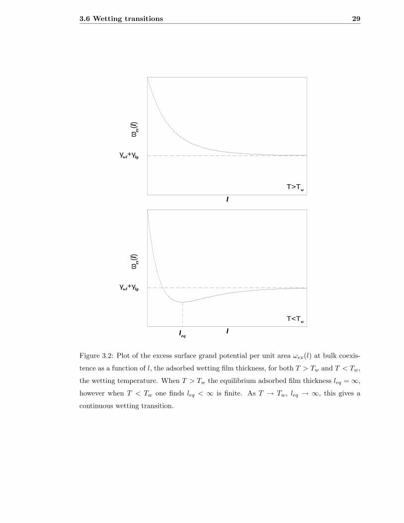
3.6 Wetting transitions 29
l
ω ex(l)
γwl+γlg
T>Tw
l
ω ex(l)
γwl+γlg
T<Tw
leq
Figure 3.2: Plot of the excess surface grand potential per unit area ωex(l) at bulk coexis-
tence as a function of l, the adsorbed wetting film thickness, for both T > Tw and T < Tw,
the wetting temperature. When T > Tw the equilibrium adsorbed film thickness leq = ∞,
however when T < Tw one finds leq < ∞ is finite. As T → Tw, leq → ∞, this gives a
continuous wetting transition.

30 A Simple Approach to Inhomogeneous Fluids and Wetting
l
ω ex(l)
γwl+γlg
T>Tw
1
l
ω ex(l)
γwl+γlg
T=Tw
1
l
ω ex(l)
γwl+γlg
T<Tw
1
leq
Figure 3.3: The excess surface grand potential per unit area, ωex(l) at bulk coexistence
as a function of l, the adsorbed wetting film thickness, for three different temperatures,
T < T 1w, T = T 1
w and T > T 1w, the wetting temperature. When T < T 1
w the equilibrium
adsorbed film thickness leq is finite, whereas for T > T 1w, leq = ∞. At T 1
w the equilibrium
wetting film thickness diverges discontinuously to infinity.

3.6 Wetting transitions 31
regime where both A(T ) and B(T ) in Eq. (3.6.2) are positive, then one finds that for small
δµ, leq is given by
leq ' −ξ ln
(
ξ(ρl − ρg)δµ
A(T )
)
. (3.6.3)
Thus as one approaches coexistence at constant temperature, the adsorbed film thickness
diverges: l ∼ −ξ ln δµ. This result, which applies for fluids interacting via short ranged
pair potentials and short-ranged wall-fluid potentials, is not just a feature of the present
Landau treatment of wetting. The same result appears in more sophisticated (albeit still
mean-field) treatments, for example in DFT treatments of wetting [11].
When the wetting transition is first order we saw that there was a discontinuous jump
(divergence) in the adsorbed film thickness at the wetting transition. This jump also
manifests itself off-coexistence: For a first order wetting transition one finds a pre-wetting
line. This line starts at the wetting transition point, T = T 1w, and extends away from the
liquid-gas coexistence line, ending in a critical point at a higher temperature Twcp > T 1w.
If one considers a path approaching the liquid-gas coexistence line, at the point where
this path intersects the pre-wetting line the adsorption at the wall is discontinuous. The
adsorbed film thickness jumps from one finite value to another larger but finite value (both
values are finite since neither state points are on the bulk liquid-gas coexistence line). The
pre-wetting line is therefore a line of first order (thin-thick adsorbed film) surface phase
transitions. It meets the bulk coexistence line tangentially at T = T 1w. In Fig. 3.4 (see also
Fig. 2.2 in Ref. [11]) we plot the adsorbed film thickness, leq, for three different paths (at
three temperatures), intersecting the liquid-gas coexistence line at chemical potential µsat.
In the inset is plotted a typical pre-wetting line (end-points marked with filled circles), on
the phase diagram for the fluid in the chemical potential-temperature, (µ, T ), plane. For
a temperature T < T 1w, the wetting temperature, (path A) the adsorbed film thickness
remains finite right up to coexistence. On path B, intersecting the pre-wetting line, there
is a discontinuity in the adsorbed film thickness at the point where this path intersects the
pre-wetting line. On path B and on path C, at a temperature above Twcp, the pre-wetting
line critical point, the adsorbed film thickness diverges continuously as µ → µ−sat.
Another issue we have not addressed in this introduction to wetting of fluids composed
of particles interacting via short ranged forces is what is the effect of wall potentials that
are not delta function-like, as we assumed so far? If we set the external potential in Eq.
(3.5.2) to be of the form V>(z) = εδ(z)+ ν exp(−z/λ), where λ is the wall potential decay

32 A Simple Approach to Inhomogeneous Fluids and Wetting
µ
leq
µsat
A B C
µ
µsat
T
Tw
1Twcp
A
B
C
Figure 3.4: The equilibrium film thickness leq for three different paths at three different
temperatures. The paths are marked in the fluid phase diagram in the inset. Path A is at
a temperature T < T 1w, below the wetting temperature Tw. On this path the adsorbed film
thickness remains finite right up to coexistence. On path B, intersecting the pre-wetting
line (filled circles at the ends), the film thickness is discontinuous at the point where this
path intersects the pre-wetting line. On path B, leq → ∞ as µ → µ−sat. On path C,
leq also diverges as µ → µ−sat. However for this temperature, T > Twcp, above the pre-
wetting line critical point temperature, there is no jump at lower values of µ. Note that
for simplicity we have assumed that the bulk coexistence value of the chemical potential
µsat is independent of temperature.
length, this will add a term
νL−3
∫ ∞
0dz exp(−z/λ)φ(z) (3.6.4)
to wex in Eq. (3.5.3). When the adsorbed wetting film thickness is large, then this will
just add terms ' Awall(T ) exp(−l/λ) + O(exp(−2l/λ)) to Eq. (3.6.2):
ωex(l) = γwl + γlg + l(ρl − ρg)δµ + A(T ) exp(−l/ξ) + B(T ) exp(−2l/ξ)
+ Awall(T ) exp(−l/λ) + O[exp(−3l/ξ), exp(−2l/λ)]. (3.6.5)
In this situation there are now three competing length scales, λ, ξ and ξ/2. This can affect
the type of wetting transition and can give rise to non-universal exponents for critical

3.6 Wetting transitions 33
wetting [14, 15, 11]. The competing length scales can also influence how the wetting film
thickens as liquid-gas coexistence is approached. For example if λ > ξ, then the adsorbed
film thickness diverges as l ∼ −λ ln δµ, rather than with the prefactor to the logarithm
equal to ξ, which is the case in Eq. (3.6.3) [11]. If the wall potential decays faster than an
exponential, then when the adsorbed film thickness is sufficiently large, the exponential
terms in Eq. (3.6.2) will dominate any wall terms in ωex(l). However, if the wall potential
decays slower than exponential, the wall term will always dominate the terms in Eq. (3.6.2)
which are powers of exp(−l/ξ), and will determine the equilibrium adsorbed film thickness,
when l is large.
We should also mention the situation pertaining when the fluid particles interact via
pair potentials which decay algebraically such as the Lennard-Jones potential, which de-
cays ∼ r−6 as r → ∞. In this case the surface excess grand potential, Eq. (3.6.5), should
be replaced by
ωex(l) = γwl + γlg + l(ρl − ρg)δµ + A(T )l−σ + B(T )l−κ + .... (3.6.6)
where the indices σ and κ are determined by the power with which the fluid pair potentials
decay, and we have ordered σ < κ < .... As one might expect, if the wall potential also
decays algebraically, this can also add extra power law terms to Eq. (3.6.6) [11]. In the
situation where the excess grand potential is given by Eq. (3.6.6), then in the regime
where the liquid completely wets the wall, i.e. l → ∞ when δµ → 0, then the equilibrium
adsorbed film thickness diverges leq ∼ δµ−1/(σ+1) as δµ → 0 (c.f. Eq. (3.6.3)). Thus the
equilibrium film thickness divergence is a power law
leq ∼ δµ−βcos , (3.6.7)
on approaching coexistence, where the critical exponent βcos = (σ+1)−1, depends explicitly
on σ, the power of the leading term in l−1 in the surface excess grand potential (3.6.6).
For non-retarded van der Waals (dispersion) forces σ = 2 [11].
The surface excess grand potential, which can be either of the form (3.6.5) or (3.6.6),
is in general of the form [16]:
ωex(l) = γwl + γlg + γs(l, δµ), (3.6.8)
where γs is the extra contribution, which at coexistence, δµ → 0, and when there is
complete wetting, must vanish: γs → 0. γs has a ‘singular’ (non-analytic) contribution,

34 A Simple Approach to Inhomogeneous Fluids and Wetting
γsing, for δµ → 0, approaching liquid-gas coexistence. For example, when there are short
ranged forces, then l ∼ − ln δµ. Substituting this result back into Eq. (3.6.5), we find that
γsing ∼ δµ ln δµ. For long-ranged forces we find that γsing has a power law dependence
on δµ. If one goes beyond the present mean-field approach, incorporating the effects
fluctuations in the wetting film interface, then in general
γsing ∼ δµ2−αcos , (3.6.9)
where the value of the surface heat capacity exponent, αcos , depends on the form of the
wall-fluid and fluid-fluid pair potentials, even within a mean-field calculation [11].
3.7 Incorporating fluctuations
In this section we shall describe how one begins to incorporate the effects of fluctuations
in a description of wetting phenomena. So far in this introduction to wetting all the
results presented have been mean-field in nature, i.e. we have calculated the equilibrium
position, leq, of the interface between the wetting film and the bulk fluid, but we have not
considered the effects of fluctuations of the interface. We can expect the location of the
interface to wander around leq due to thermal fluctuations – these are capillary waves. In
order to go beyond mean-field we can consider small fluctuations in the location l of the
interface between the wetting film and the bulk fluid. If we think of the interface between
the wetting film and the bulk fluid as a fluctuating membrane, then the work required to
produce a distortion in the height of the membrane, l(R), at position R in the membrane
(R is a two dimensional position vector in the plane of the interface) will be equal to the
change in surface area of the membrane times the interfacial surface tension, γlg. This will
contribute a term
∆F1 = γlg
∫
dR[√
1 + (∇Rl(R))2 − 1], (3.7.1)
to the free energy. In addition to this term, since we are considering a state off-coexistence,
there will be a term due to the fact that the interface is bound to the wall. For small
fluctuations we can incorporate this if we Taylor expand the surface excess grand potential,
which in general is of the form (3.6.8), around its minimum value ωex(leq). One obtains
[10]:
ωex(l) ' ωex(leq) +1
2γlg ξ−2
‖ (l − leq)2 (3.7.2)

3.7 Incorporating fluctuations 35
where
γlg ξ−2‖ =
(
∂2ωex(l)
∂l2
)
l=leq
. (3.7.3)
The full interfacial free energy functional (or effective interfacial Hamiltonian) is thus
∆F =1
2γlg
∫
dR[(∇Rl)2 + ξ−2‖ (l − leq)
2], (3.7.4)
where we have linearised the square root in the contribution from Eq. (3.7.1) and we have
ignored the constant ωex(leq). We consider the correlation function,
C(R) ≡ 〈 (l(R) − leq)(l(0) − leq) 〉 , (3.7.5)
which is the correlation function for fluctuations in the interface between the wetting film
and the bulk fluid. Since Eq. (3.7.4) has a similar form to Eq. (3.1.3) (the difference
between the two being the dimensionality of the order parameter) which was found to
generated a correlation function with the (classical) Ornstein-Zernike form (see Eqs. (3.1.4)
– (3.1.7)), it is not surprising that the Fourier transform of C(R) is
C(Q) ∼ 1
ξ−2‖ + Q2
, (3.7.6)
and thus
C(R) ∼∫
dRexp(iQ.R)
ξ−2‖ + Q2
. (3.7.7)
We can therefore identify ξ‖ as the correlation length for fluctuations in the plane of the
interface (one can also define ξ⊥, the interfacial thermal roughness). From Eq. (3.7.3)
we can see that as bulk coexistence is approached, δµ → 0, then leq → ∞ and therefore
ξ‖ → ∞ [10, 11]. The divergence of ξ‖ as δµ → 0 is a power-law:
ξ‖ ∼ δµ−νco
‖ , (3.7.8)
where the critical exponent νco‖ is dependent on the form with which the wall-fluid and
fluid-fluid pair potentials decay [10, 11]. If we want to go beyond the Gaussian approxi-
mation for the interfacial Hamiltonian, Eq. (3.7.4), we must consider the Hamiltonian (see
Ref. [16] and references therein):
H[l(R)] =
∫
dR
[
Σ
2(∇Rl(R))2 + W (l(R))
]
, (3.7.9)
where Σ is the interfacial stiffness. To a first approximation Σ ' γlg, but in general Σ is
dependent on l. The binding potential W (l) ≡ ωex(l) − γwl − γlg (see Eq. (3.6.8)). One
36 A Simple Approach to Inhomogeneous Fluids and Wetting
finds generally that in a renormalization group treatment of fluctuation effects in (3.7.9)
that the critical exponents βcos , αco
s and νco‖ can be altered from their mean-field values.
However, for complete wetting in 3 dimensions one finds that the critical exponent values
are unchanged by fluctuations but the critical amplitudes depend upon the value of the
dimensionless parameter
ω =kBT
4πΣξ2, (3.7.10)
which controls the strength of interfacial fluctuations [11, 16].
The exponents βcos , αco
s and νco‖ which characterize the approach to complete wetting
can be related to one another using the Gibbs adsorption equation (3.3.5), plus other
surface sum rules and scaling relations. This is analogous to methods used to derive the
relations between the exponents characterizing bulk critical phenomena [11, 16]. From the
Gibbs adsorption equation
1 − αcos = −βco
s , (3.7.11)
while from a susceptibility sum rule [17, 16]
2νco‖ = αco
s . (3.7.12)
There is also a surface hyperscaling relation
2 − αcos = (d − 1)νco
‖ , (3.7.13)
where d is the dimensionality of the system. Within a mean-field treatment, for short
ranged forces, the critical exponents are:
αcos = 1, βco
s = 0 (ln), νco‖ =
1
2(3.7.14)
in d = 3. There is also a set of (different) exponents characterizing the wetting transition
point, however these are beyond the scope of the present basic introduction to wetting,
and we refer the reader to the literature – see Refs. [11, 16, 18], and references therein.

Chapter 4
The One Component
Gaussian Core Model
The Gaussian core model (GCM) is a simple model for polymers in a good solvent. The
effective pair potential between the centers of mass of the polymers is modeled by a repulsive
Gaussian potential. In this chapter we provide a brief introduction to some of the existing
results for the structure and thermodynamics of this model fluid. Since the GCM pair
potential is purely repulsive, the one-component fluid does not exhibit liquid-gas phase
separation, however the GCM does freeze and we present a simple theory for the phase
diagram of the one-component GCM.
4.1 Introduction: effective interactions
The GCM consists of a set of classical particles each interacting with a repulsive pairwise
potential given by:
v(r) = ε exp(−r2/R2), (4.1.1)
where ε > 0 and R is a length scale determining the size of the particles. In the next
section we will describe briefly some simulation results which form the basis for viewing
the GCM as a simple model for polymers dissolved in an athermal solvent, with Eq.
(4.1.1) representing the effective interaction between the centers of mass of the individual
polymer chains. This ‘colloid’ approach to polymers [19, 20, 21] represents a significant
simplification in the description of a polymer solution. Formally one would calculate the
effective potential between the polymers by integrating over the internal (monomeric)
37

38 The One Component Gaussian Core Model
degrees of freedom in the partition function, so that the partition function is in the form
of a trace over the Boltzmann factor of an effective Hamiltonian which is only a function
of the center of mass coordinates. In doing this, the effective Hamiltonian no longer
contains just pairwise terms, even when the underlying monomer-monomer interactions
are pairwise. In general the effective Hamiltonian is made up of a sum of terms, the first
of which does not depend on the polymer coordinates; the second is a one body quantity
which is a function of a single polymer coordinate; the third is a pairwise term, involving
pairs of the polymer center of mass coordinates; the fourth is a three-body term and so
on, with each successive term depending on increasing numbers of particle coordinates
[22, 23, 24]. This sum is often truncated at the pair terms in order to render the system
tractable. Although the GCM is not derived in such a manner, the Gaussian potential is
an approximation at the pairwise level for the effective interaction between the centers of
mass of the polymers in solution1.
4.2 A simple model for polymers in solution
When a polymer is in solution, each polymer chain is free to move around. If the solvent
is a poor solvent, i.e. when the attraction between the monomers, which make up the
polymer chain, is stronger than the attraction between the solvent molecules and the
monomers, then each polymer chain tends to collapse and to form a dense bundle, as it
minimizes the contact with the solvent. However in a good solvent, the polymer chain
opens up, to maximize the contact with the solvent molecules [22, 25]. In fact there is an
effective repulsion between the monomers of the polymer, and the chain statistics can be
well modeled by a self avoiding random walk. In a good solvent, each polymer chain can,
on a coarse grained length scale and on time scales greater that that associated with the
fluctuations of the polymer coils, be modeled as a ‘blob’, characterized by a mean position
(the center of mass of the polymer) and by a typical size, the radius of gyration – see Fig.
4.1. This is the view of polymer solutions that we shall take in this thesis.
A Gaussian effective potential for polymers was first proposed by Flory and Krigbaum
[26], and most recently, it this aspect of the model that has generated the most interest.
1One is not restricted to using the center of mass coordinates for the position of the polymer. One
could, for example, use the coordinates of the central monomer in the polymer chains. In fact this approach
is more fruitful for star-polymers – this is the approach we take in chapter 8.
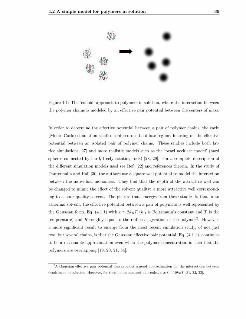
4.2 A simple model for polymers in solution 39
Figure 4.1: The ‘colloid’ approach to polymers in solution, where the interaction between
the polymer chains is modeled by an effective pair potential between the centers of mass.
In order to determine the effective potential between a pair of polymer chains, the early
(Monte-Carlo) simulation studies centered on the dilute regime, focusing on the effective
potential between an isolated pair of polymer chains. These studies include both lat-
tice simulations [27] and more realistic models such as the ‘pearl necklace model’ (hard
spheres connected by hard, freely rotating rods) [28, 29]. For a complete description of
the different simulation models used see Ref. [22] and references therein. In the study of
Dautenhahn and Hall [30] the authors use a square well potential to model the interaction
between the individual monomers. They find that the depth of the attractive well can
be changed to mimic the effect of the solvent quality: a more attractive well correspond-
ing to a poor quality solvent. The picture that emerges from these studies is that in an
athermal solvent, the effective potential between a pair of polymers is well represented by
the Gaussian form, Eq. (4.1.1) with ε ' 2kBT (kB is Boltzmann’s constant and T is the
temperature) and R roughly equal to the radius of gyration of the polymer2. However,
a more significant result to emerge from the most recent simulation study, of not just
two, but several chains, is that the Gaussian effective pair potential, Eq. (4.1.1), continues
to be a reasonable approximation even when the polymer concentration is such that the
polymers are overlapping [19, 20, 21, 34].
2A Gaussian effective pair potential also provides a good approximation for the interactions between
dendrimers in solution. However, for these more compact molecules, ε ' 8 − 10kBT [31, 32, 33].

40 The One Component Gaussian Core Model
0 1 2 3r/R
0
0.25
0.5
0.75
1
g(r)
Figure 4.2: The radial distribution function, g(r), for the GCM with ε∗ = 2 calculated
using the quasi-exact (when compared with simulations) HNC closure to the OZ equation
(dashed line) and with the RPA closure (solid line). These are calculated for fluid densities
ρR3 = 0.5, 2, 4 and 6 (from bottom to top). Note that the RPA closure provides an
increasingly accurate approximation for g(r) as the density is increased. g(r) displays a
deep correlation hole, for r → 0, at the lower densities, but as ρR3 → ∞, then g(r) → 1
for all values of r.
4.3 Properties of the one-component GCM fluid
An excellent review of the properties of the GCM can be found in Ref. [22] but for com-
pleteness we shall mention some of the properties here. The GCM was introduced in the
mid-seventies by Stillinger [35], and was of interest because the GCM can yield a negative
thermal expansion coefficient in the liquid phase [36]. The phase behaviour of the GCM
is rather well established [22, 36, 37]; in the temperature-density (T, ρ) plane there is a
region below kBT/ε ' 0.01 where increasing ρ leads to freezing into a fcc phase, followed
by a fcc-bcc transition and then melting so that the fluid is stable at high densities. For
ε∗ ≡ βε < 100, where β = (kBT )−1, the fluid is stable at all densities. Recently Lang
et al. [37, 38] and Louis et al. [39] have studied the fluid region of the phase diagram
using Monte Carlo simulations and integral equation theories. What emerges is that for
high densities the hypernetted-chain (HNC) approximation provides an excellent account

4.3 Properties of the one-component GCM fluid 41
of the Monte Carlo results for the radial distribution function g(r), structure factor S(q)
and the equation of state and therefore the HNC approximation is viewed as being quasi-
exact for the GCM. In the limit ρR3 → ∞ it is argued that the HNC closure should
become exact [37, 38]. Particularly striking is the observation that a very simple closure,
the random phase approximation (RPA) which sets the pair direct correlation function
c(2)(r) = −βv(r), becomes very accurate for very high densities: ρR3 & 5 [37, 38, 39]3.
This implies that the GCM behaves as a ‘mean-field fluid’ over a very wide density and
temperature range. In Fig. 4.2 we plot the results for g(r) from the HNC and RPA clo-
sures to the OZ equation. One can see that as the density increases the correlation hole
at small values of r is reduced and g(r) → 1, for all separations of the particles. Such be-
haviour is very different from that of fluids with hard-cores, where short-ranged (packing
induced) correlations always persist [1]. For this soft-core model in the limit ρR3 → ∞,
the mean inter-particle separation ρ−1/3 becomes ¿ R and a central particle interacts
with a very large number of neighbours – a classic mean-field situation. However, for low
temperatures and densities, this picture does not hold, the particle interactions become
increasingly hard-sphere like as the temperature T → 0 and the correlation functions for
the GCM are well approximated by those of a hard-sphere fluid [22, 36]. The reason
for this behaviour is as follows: In the partition function the pair potential appears as a
Boltzmann factor. The Boltzmann factor of the GCM pair potential is
B(r, β) = exp[−βε exp(−r2/R2)]. (4.3.1)
B is a monotonic function of the interparticle distance r. The separation r∗ at which
B = 12 is
r∗(β) = R
√
ln
(
βε
ln 2
)
, (4.3.2)
and the gradient of the Boltzmann factor at this point is:
(
dB
dr
)
r=r∗=
ln 2
R2r∗(β), (4.3.3)
so as β → ∞, both r∗ and (dB/dr)r=r∗ diverge; i.e. the Gaussian particles behave more
and more like hard-spheres as the temperature is decreased, with an effective hard-sphere
radius equal to r∗ [22, 36]. This argument, of course, only applies in the regime where the
3By making comparison with simulations C.N. Likos et al. [38] have established the validity of the RPA
at high densities for bounded, positive definite pair potentials in general.

42 The One Component Gaussian Core Model
0 2 4 6 8 10r/R
0
0.5
1
1.5
2
g(r)
Figure 4.3: The radial distribution function, g(r), calculated using the HNC closure to the
OZ equation for a GCM fluid with density ρR3 = 0.1 at a temperature kBT/ε = 0.01 (solid
line) and at kBT/ε = 0.5 (dashed line). Note that g(r) at low temperatures resembles that
of a hard-sphere fluid, whereas at higher temperatures g(r) is completely different and is
much less structured.
GCM fluid density is less than that at which hard-spheres of radius r∗ close pack. In Fig.
4.3 we display the radial distribution function, g(r), calculated using the HNC closure to
the OZ equation for a GCM fluid with density ρR3 = 0.1 at a temperature kBT/ε = 0.01
(solid line) and at kBT/ε = 0.5 (dashed line). In the low temperature and density regime
g(r) is much more structured; the fluid is near to freezing and g(r) is similar to that for
a hard-sphere fluid. However at higher densities and/or temperatures, the particle cores
overlap and g(r) is much less structured. It is in this overlap regime that the RPA is a
good approximation to make for the fluid correlation functions.
Since the RPA is accurate over such a large range of bulk densities it is tempting to
argue [22, 37, 39] that the simple mean-field Helmholtz free energy functional, Eq. (2.3.25),
should yield a realistic description of the inhomogeneous GCM fluid, provided the one-body
density ρ(r) does not acquire very small values. The density functional (2.3.25) generates
the RPA: c(2)(r) = −βv(r). Physically one is arguing that the excess (over the ideal gas
Fid) free energy of the fluid can be approximated by the internal energy with the pairwise

4.4 Solid phases of the GCM 43
distribution function ρ(2)(r1, r2) replaced by its uncorrelated limit ρ(r1)ρ(r2). Louis et al.
used the functional (2.3.25) to investigate the density profiles of GCM particles adsorbed
at a hard wall. Their results agree closely with results from Monte Carlo simulations and
with the results from the HNC DFT [39, 7] for the GCM with ε∗ = 2, both for a hard
planar wall (i.e. the wall potential Vext(z) = ∞ for z < 0 and Vext(z) = 0 for z > 0)
and also for an external potential of the form βVext = exp(−z)/z, at three bulk densities
ρR3 = 1, 0.5, 0.1, confirming that the GCM does behave as a ‘mean-field fluid’ – at least
for this type of inhomogeneity [39].
4.4 Solid phases of the GCM
By performing lattice sums to determine the free energy for candidate solid phases of
the GCM, and by molecular dynamics simulations, Stillinger and co-workers were able to
determine the form of the GCM phase diagram [35, 36, 40, 41, 42, 43]. They found that
there are two equilibrium solid phases: fcc at lower densities and bcc at higher densities.
They also established a novel feature of the GCM: that the solid undergoes re-entrant
melting, i.e. if one fixes the temperature, for example choose kBT/ε = 0.004, then as one
increases the density, the fluid first freezes, but then as the density is further increased the
crystal melts again and there are no further freezing transitions. This scenario is particular
to some soft core systems, where the equilibrium phase at high densities is a liquid, rather
than a solid. Note also that a solid with multiple occupancies on each lattice site is not
the equilibrium phase for the GCM.
More recently Lang et al. [37] used a different method for calculating the GCM phase
diagram. They adopted an Einstein-model approach [44], based on the Gibbs-Bogoliubov
inequality, which relates the Helmholtz free energy F of a system with Hamiltonian H, to
that of a reference system, F0, with Hamiltonian H0:
F ≤ F0 + 〈H − H0〉0 . (4.4.1)
For the reference system, Lang et al. [37] used the Einstein model of a solid, which has
the following Hamiltonian:
H0 =N
∑
i=1
[
p2i
2m+ α(ri − Ri)
2
]
, (4.4.2)
where i labels the particles, each of which has mass m, position ri and momentum pi. Each
particle is bound by a harmonic potential to a lattice site at Ri. The ‘spring constant’

44 The One Component Gaussian Core Model
α for the harmonic potential is treated as a variational parameter. The Helmholtz free
energy for the Einstein solid is simply (see Appendix A)
F0 = 3NkBT ln
(
φΛ√πR
)
(4.4.3)
where the dimensionless parameter
φ =√
βαR2 (4.4.4)
and F0 is, of course, independent of the length scale R. Within the Einstein model the
one body density is simply a sum of Gaussian profiles, each centered on the lattice sites:
ρE(r) =∑
i
φ3
π3/2R3e−φ2|r−Ri|
2/R2
, (4.4.5)
and the two-body density is a sum of products of Gaussians:
ρ(2)E (r, r′) =
∑
i6=j
φ6
π3R6e−φ2|r−Ri|
2/R2
e−φ2|r′−Rj |2/R2
. (4.4.6)
From the Gibbs-Bogoliubov inequality (4.4.1) one obtains the following upper bound for
the Helmholtz free energy [1, 44]
F ≤ F0 +1
2
∫
dr
∫
dr′ ρ(2)E (r, r′)v(|r − r′|) − 3
2NkBT. (4.4.7)
The final term is obtained simply by applying the equipartition theorem for the three
potential energy (configurational) degrees of freedom in reference Hamiltonian (4.4.2). On
substituting Eq. (4.4.6) into (4.4.7), one can perform the simple integrals, since the GCM
pair potential v(r) in Eq. (4.4.7) is a Gaussian, and one obtains:
F ≤ F ≡ F0 +Nεφ3
2(φ2 + 2)3/2
∑
ν
mν exp
(
− a2ν
R2(1 + 2/φ2)
)
− 3
2NkBT, (4.4.8)
where the index ν denotes a sum over lattice vectors aν = Ri − Rj , with magnitude
|aν | = aν . mν is an integer denoting the number of lattice vectors of length aν belonging
to a shell. The only parameter in Eq. (4.4.8) is the width parameter φ of the Gaussian
density peaks, which is treated as a variational parameter, to be determined from the
minimization condition ∂F /∂φ = 0, and one assumes that F = minF . One can therefore
calculate the Helmholtz free energy for any trial crystal structure; one simply inputs the
sets of mν and aν(ρ) for the particular lattice structure into Eq. (4.4.8) and then minimizes
with respect to φ. Lang et al. [37] calculated the free energy for various crystal structures

4.4 Solid phases of the GCM 45
Figure 4.4: The phase diagram for the one component GCM calculated by Lang et al. [37]
(taken with kind permission), plotted in the reduced temperature t = kBT/ε versus density
ρ plane (note: σ ≡ R). The two insets (a) and (b) show details of the phase diagram. The
low density equilibrium solid phase is the fcc crystal, and at higher densities it is the bcc
crystal. On increasing the temperature or the density, the fluid is the equilibrium phase.
and found, as one would expect based on the results of Stillinger and co-workers [35], that
the only equilibrium crystal phases for the GCM were those with the fcc and bcc lattices.
In order to calculate the fluid free energy Lang et al. [37] used the HNC virial route.
In order to implement this approach one uses the HNC closure to the OZ equation to
calculate the radial distribution function for the fluid, g(r), along a path at constant
temperature in the phase diagram, starting from the point with density ρ = 0 and ending
at the point with density ρ in the phase diagram, where the fluid free energy is required.
One then inputs the HNC g(r) to the virial equation (2.1.16) to calculate the pressure
of the fluid, P . By integrating the thermodynamic relation P = −(∂F/∂V )T along the
path in the phase diagram, one can determine the fluid free energy Ffluid(ρ). In order to
calculate the coexisting densities between any two phases (either the fluid, or the bcc and
fcc solid phases) the common-tangent construction was performed between the Ffluid/V
and Fsolid/V curves. Their resulting phase diagram is displayed in Fig. 4.4. Note that the
thermodynamic state point of the fluid or solid is completely determined by the average
density of the system 〈ρ(r)〉 = ρ = N/V and by the reduced temperature kBT/ε. The low
density equilibrium solid phase is the fcc crystal, and at higher densities, ρR3 & 0.17, it is

46 The One Component Gaussian Core Model
the bcc crystal that is the equilibrium solid phase. On increasing the temperature or the
density, the fluid is the equilibrium phase. The difference in density between the coexisting
phases are all relatively small – see the insets to Fig. 4.4. For example the difference in
density between the coexisting fcc and bcc solid phases is independent of temperature,
(ρbcc − ρfcc)R3 = 3.6 × 10⁻⁴ [37].
4.5 DFT theory for the solid phases of the GCM
Here we present a simple alternative (DFT) method for determining an approximate phase
diagram for the one component GCM. The RPA excess Helmholtz free energy functional
F [ρ] = Fid[ρ] +1
2
∫
dr
∫
dr′ ρ(r) ρ(r′)v(|r − r′|), (4.5.1)
where the ideal gas part of the free energy functional is
Fid[ρ] = kBT
∫
dr ρ(r) [ln(Λ3ρ(r)) − 1], (4.5.2)
provides an accurate approximation for the fluid free energy when the fluid is at temper-
atures and densities such that the soft cores of the particles are overlapping. However, as
we have seen, the RPA functional generates correlation functions which fail to describe
correctly the correlations in the fluid when it is near to freezing. The approximation lead-
ing to Eq. (4.5.1) assumes that there are multiple overlaps between the particles. However,
in the regime where the particles freeze the repulsion between the GCM particles is suf-
ficient for the correlations between the particles to be better approximated by particles
with hard (impenetrable) cores – see Fig. 4.3. We therefore expect Eq. (4.5.1) to provide
a poor approximation to the free energy of the GCM liquid in this region of the phase
diagram. However, perhaps surprisingly, we find that an RPA-like approximation provides
a good approximation for the Helmholtz free energy of the solid phases.
When in the fluid state, the one-body density is a constant, ρ(r) = ρ. However,
when the system freezes into a solid, the density is periodic, i.e. the symmetry breaks and
ρ(r) = ρ(r−Ri), where Ri is a lattice vector for the solid phase. An approximation that is
often made in DFT studies of freezing [45, 22], is to assume that the density profile of the
solid is made up of Gaussian peaks, of the form in Eq. (4.4.5). This density profile assumes
a normalization condition: i.e. there is one particle per lattice site. This assumption need
not necessarily be true. We can expect to find vacancies in the crystal, and indeed for the

4.5 DFT theory for the solid phases of the GCM 47
present soft core system we may find another type of defect: double occupancy, since the
particle cores can overlap. However, we expect the proportion of defects to be small, and
assume therefore a perfect crystal. In fact, at high densities, where there is a tendency
towards double occupancy, we find that for the present soft core system there is re-entrant
melting: at high densities the fluid is the stable phase rather than a multiple occupied
solid.
If we assume the crystal density is of the form given by Eq. (4.4.5), with φ taking a value
sufficiently large that the overlap between the Gaussian density peaks on neighbouring
lattice sites can be assumed to be negligible, then the ideal gas part of the Helmholtz free
energy, Eq. (4.5.2), is simply
F solidid (ρ, φ) = NkBT
[
3 ln
(
Λφ√πR
)
− 5
2
]
, (4.5.3)
which is independent of R. It is interesting to note that this differs from the free energy
of the Einstein solid, Eq. (4.4.3), solely by a (φ independent) amount, 52NkBT , this is
discussed further in Appendix A. We approximate the mean-field Helmholtz free energy
by:
F (ρ) = F solidid (ρ, φ) +
φ6
2π3R6
∑
i6=j
∫
dr
∫
dr′ e−φ2|r−Ri|2/R2
e−φ2|r′−Rj |2/R2
v(|r − r′|).
(4.5.4)
Note that this result is not exactly that which would arise from inserting the profile Eq.
(4.4.5) into the RPA functional Eq. (4.5.1); we have omitted from the sum over lattice
sites all the terms where the index i = j. The result can be viewed as an RPA-like
approximation derived from Eq. (2.3.24) by assuming that the two body density is of the
form in Eq. (4.4.6) for all values of the charging parameter α in Eq. (2.3.24).
The integrals in Eq. (4.5.4) are exactly the same as those in Eq. (4.4.7), and so we
obtain:
Fsolid(ρ, φ) = F solidid (ρ, φ) +
Nεφ3
2(φ2 + 2)3/2
∑
ν
mν exp
(
− a2ν
R2(1 + 2/φ2)
)
. (4.5.5)
This expression is almost the same as that obtained in the previous section using a theory
based on the Einstein model for the free energy of the solid phases, except the expression
in Eq. (4.4.8) and that in Eq. (4.5.5) differ by NkBT . This difference originates from the
presence of the 1/N ! indistinguishability factor in the partition function that formed the
(liquid state theory) basis for Eqs. (4.5.1) and (4.5.2), from which Eq. (4.5.5) is derived.

48 The One Component Gaussian Core Model
By contrast, in the Einstein model the particles are fixed to the lattice sites and are
therefore distinguishable – see Appendix A for a more detailed discussion of these issues.
However, for our present purposes this (φ independent) difference has no effect, because in
the present approach all solid phases have this additional term, and we use a Lindemann
criterion to calculate the solid melting curves, rather than compare our solid free energy
with that of the liquid, which is the situation in which this term would matter.
We approximate Eq. (4.5.5) by truncating the sum over lattice vectors to a sum over
nearest neighbours and next nearest neighbours only. The only parameter in Eq. (4.5.5)
is the width of the Gaussian density peaks φ and, as in the previous section, we treat this
as a variational parameter, determined from the minimization condition ∂Fsolid/∂φ = 0.
Based on information from earlier studies [22, 36, 37] for the phase diagram of the GCM,
we calculated only the free energy for the bcc and fcc crystal structures. Some typical
plots of the free energy as a function of φ are displayed in Fig. 4.5. We find that the free
energy always has a minimum at φ = 0, this corresponds to the fluid state, where the
particles are completely delocalized. However, for some points in the phase diagram the
free energy has a second minimum at some other (non-zero) value of φ, and this is the
value we use to calculate the free energy.
The usual procedure for determining the phase diagram, once the free energy density
for all the trial phases has been calculated, is to perform the common tangent construction
(which is equivalent to equating chemical potentials and pressures in the coexisting phases)
in order to find the coexisting state points between the different phases. We find, as did
Lang et al. [37], that the free energy for the fcc solid is lower than that for the bcc at
low densities (ρR3 . 0.16). We could therefore perform the common tangent construction
between these two free energies and determine the coexisting densities. However, due to
the soft core nature of the present system, the density change at the transition is very small
– see the inset to Fig. 4.4 and Ref. [37], and since we are mostly interested in providing a
simple theory which accounts for the topology of the phase diagram, we simply determined
the density at which the Helmholtz free energy of the bcc equals that of the fcc structure
for a given temperature. The resulting line is plotted in Fig. 4.6.
In order to calculate the fluid-solid coexistence we should calculate the fluid Helmholtz
free energy density and perform the common tangent construction between this and the
solid phase free energy. However, the integral equation procedure used by Lang et al. [37]
is numerically intensive, and at the low temperatures and densities at which the GCM

4.5 DFT theory for the solid phases of the GCM 49
0 5 10 15 20φ
f fcc
*10−1
A
B
C
Figure 4.5: The Helmholtz free energy (in arbitrary units) for an fcc lattice as a function
of φ, the localization parameter. Results are calculated at ρR3 = 0.12 and kBT/ε = 0.004
(labeled A), at ρR3 = 0.04 and kBT/ε = 0.004 (B) and at ρR3 = 0.7 and kBT/ε = 0.01
(C). Note that C is multiplied by a factor 10−1. A has a minimum at φ = 6.63, B a
minimum at φ = 1.89 and for C there is no minimum at all (except the trivial minimum
at φ = 0 which denotes a solution where the particles are completely delocalized). A is
calculated at a state point inside the region where we expect the fcc to be the equilibrium
phase, whereas B and C correspond to points where the fluid is the equilibrium phase.
freezes, we are unable to use the RPA Helmholtz free energy, since it provides a very poor
estimate for the free energy of the fluid in this region of the phase diagram. It greatly
over estimates the fluid free energy.
Here we will use a different method to determine the melting temperature of the solid,
namely the Lindemann criterion: the crystal melts when the ratio of the root-mean-square
displacement, σ ≡ (⟨
r2⟩
−〈r〉2)1/2, of the particle about its equilibrium position is roughly
10% of the nearest neighbour distance, a1. This is simple to implement for the Gaussian
profile, Eq. (4.5.5) which gives σ =√
32(R
φ ). For the fcc crystal afcc1 = 21/6ρ−1/3, and
we choose the (somewhat arbitrary)4 Lindemann criterion for when the fcc melts to be
4In Ref. [43], Stillinger and Weber used molecular dynamics simulations to determine the temperature
when the GCM fluid with density ρR3 = 0.2 melts. Their Lindemann ratio was σ/a1 = 0.16. This value

50 The One Component Gaussian Core Model
0 0.2 0.4 0.6 0.8ρR
3
0
0.002
0.004
0.006
0.008
0.01
0.012
0.014
k BT
/ε
fcc
bcc
fluid
Figure 4.6: The phase diagram of the one component GCM. Rather than calculate the
phase boundaries by performing the common tangent construction between the free energy
densities of the competing solid phases, the fcc-bcc transition line is given by the locus
of points where the Helmholtz free energies of the two phases are equal. The melting
boundaries are determined using the Lindemann criterion – see the text.
φafcc1 /R = 12.2 (i.e. when σ/afcc
1 = 0.100). Similarly for bcc abcc1 = 2−2/3
√3ρ−1/3 and we
choose the Lindemann criterion for when the bcc melts to be φabcc1 /R = 11.8 (i.e. when
σ/abcc1 = 0.104). This second (slightly different) value for the bcc Lindemann criterion is
chosen so that the melting lines for the bcc and fcc phases form a continuous boundary line
between the fluid and solid phases. The plot of the resulting phase diagram is displayed
in Fig. 4.6. Remarkably, all the transitions in Fig. 4.6 are located within 20% of the
locations found in the more sophisticated approach of Lang et al. [37] – see Fig. 4.4. The
main difference between Fig. 4.6, and the more accurate phase diagram in Fig. 4.4 is in
the location of the bcc-solid melting transition line. This is because as the GCM density
increases our approximation of truncating the sum over lattice vectors after nearest and
next nearest neighbour contributions only in Eq. (4.5.5), becomes increasingly inaccurate.
is larger than the criterion we use here. Within the present theory there is not always a minimum of Eq.
(4.5.5) for σ/a1 = 0.16. It is well known that DFT theories for solids often under-estimate the value of the
Lindemann ratio [46].

4.5 DFT theory for the solid phases of the GCM 51
This can be seen particularly in the tail of the fluid-bcc boundary for densities ρR3 > 0.6.
In order to improve the theory one should include further terms in the sum in Eq. (4.5.5).
However, our main purpose in truncating the sum was to construct a simple theory and
also to demonstrate that it is the nearest and next nearest neighbour contributions in Eq.
(4.5.5) which dominate this expression for the Helmholtz free energy of the solid phases
of the GCM. Another criterion that we used for determining the melting curves was to
calculate the locus of points where there is no longer a solution φ 6= 0 to the equation
∂Fsolid/∂φ = 0, still using Eq. (4.5.5) to determine Fsolid. This results in a phase diagram
with the same topology as Fig. 4.6, but is, of course, a much less accurate method than
that based on the Lindemann criterion.
Having given a brief overview of some of the properties of a one component fluid of
GCM particles, in the next chapter we shall describe some of the properties of a binary
fluid of GCM particles, the main topic of this thesis.

Chapter 5
The Binary Gaussian Core Model:
Fluid-Fluid Phase Separation and
Interfacial Properties
Using a mean-field equation of state we calculate the density-concentration phase diagrams
for a binary mixture of repulsive Gaussian core particles over a range of size ratios. A
simple RPA mean-field DFT approach is used to calculate the surface tension and den-
sity profiles of the interface between the demixed fluid phases of the binary mixture. For
certain coexisting states oscillations are found in the density profiles on both sides of the
interface, i.e. approaching both bulk phases. The form of the oscillations is determined by
the asymptotic decay of the bulk total pairwise correlations and the onset of oscillations in
the interfacial density profiles is linked to the location of the crossover line (Fisher-Widom
line) in the bulk phase diagram where the asymptotic decay changes from monotonic to
damped oscillatory. For certain particle size ratios we find a new crossover line which
separates a region of the phase diagram where the longest range decay of the pairwise
correlations is damped oscillatory from a region where the longest range decay is damped
oscillatory but with a different wavelength. We argue that many of the predictions of the
simple DFT approach should remain valid in more refined treatments.
Given the success of the simple mean-field RPA Helmholtz free energy functional
(2.3.25) in describing the pure fluid it is natural to ask what the corresponding theory
yields for a binary mixture of repulsive Gaussian core particles. This question was ad-
dressed partially in Refs. [39, 47] and the authors showed that for certain choices of the
53

54 Binary GCM: Fluid-Fluid Phase Separation and Interfacial Properties
energy and range parameters fluid-fluid demixing is predicted by the mean-field (RPA)
approach. Although it is not clear that this phase separation mimics that which is found
in polymer blends [39], the observation that a system with purely repulsive inter-particle
potentials can separate into two fluid phases is of intrinsic interest. Recall that the pure
GCM exhibits only a single fluid phase.
5.1 Demixing in binary fluids
Before considering demixing in binary fluids, we shall remind the reader about phase
separation in one-component fluids. A simple one-component fluid can separate into two
coexisting phases, a liquid and a gas. For these two phases to coexist the chemical potential
µ and the pressure P must be equal in the two phases – i.e. the two phases must be in
chemical and mechanical equilibrium. In any theory for a fluid, phase separation manifests
itself as a convex portion in the Helmholtz free energy curve, i.e. the free energy per particle
f = F/N , as a function of the volume per particle v = V/N has a convex portion. If f(v) is
convex, then the fluid with density ρ = 1/v, will be unstable to density fluctuations, since
in this region the isothermal compressibility χT , given by Eq. (2.1.14), will be negative.
The boundary to this unstable region is the spinodal and is defined as the locus of points
where χ−1T = 0, i.e. where
∂2f
∂v2= 0. (5.1.1)
One finds that the two points on the curve f(v), corresponding to the coexisting liquid
and gas, are outside the unstable region, one either side. These points are determined as
follows: The pressure in the fluid is given by
P (v) = −(
∂F
∂V
)
N
= −(
∂f
∂v
)
(5.1.2)
and the chemical potential
µ(v) =
(
∂F
∂N
)
V
= f(v) − v
(
∂f
∂v
)
. (5.1.3)
If the densities of the coexisting liquid and gas phases are v−1l and v−1
g respectively, then
from the conditions of mechanical equilibrium P (vl) = P (vg) and of chemical equilibrium
µ(vl) = µ(vg) one obtains:
∂f
∂v
∣
∣
∣
∣
∣
vl
=∂f
∂v
∣
∣
∣
∣
∣
vg
=f(vl) − f(vg)
vl − vg, (5.1.4)

5.1 Demixing in binary fluids 55
which geometrically corresponds to the common tangent construction on the curve f(v).
The locus of points in the phase diagram defined by (5.1.4) is known as the binodal. The
binodal meets the spinodal at a single point (temperature), the bulk critical point. This
is the only point in the fluid phase diagram where there is an equilibrium phase with the
compressibility χT = ∞.
Extending the above ideas to a binary fluid is now straight-forward. A fluid composed
of two different species of particles (labeled 1 and 2) can separate into two demixed phases,
A and B, one rich in species 1 and the other poor in species 1. For phases A and B to be
in equilibrium, the chemical potentials µi and the pressure P of the two phases must be
equal, i.e. µi,A = µi,B for i = 1, 2 and PA = PB. The variables we work with are the total
density ρ and a composition variable x, such that the bulk densities of the two species are
ρb1 = (1 − x)ρ and ρb
2 = xρ. In terms of v = 1/ρ, the volume per particle, the chemical
potentials and pressure are:
µ1 = f − v
(
∂f
∂v
)
x
− x
(
∂f
∂x
)
v
(5.1.5)
µ2 = f − v
(
∂f
∂v
)
x
+ (1 − x)
(
∂f
∂x
)
v
(5.1.6)
P = −(
∂f
∂v
)
x
. (5.1.7)
The calculation of the binodal is simpler to perform in the ensemble where the pressure is
the independent variable instead of the total density ρ = 1/v. We Legendre transform to
g = f + Pv where g(x, P ) is the Gibbs free energy per particle. In this ensemble the con-
ditions of equal chemical potential and pressure lead to the common tangent construction
on g:(
∂g
∂x
)
P
∣
∣
∣
∣
∣
xA
=
(
∂g
∂x
)
P
∣
∣
∣
∣
∣
xB
=g(xA, P ) − g(xB, P )
xA − xB(5.1.8)
where xA and xB are the concentrations of species 2 in phases A and B respectively. The
spinodal is now the locus of points at which
(
∂2g
∂x2
)
P
= 0. (5.1.9)
Note that all derivatives are performed at constant temperature T .

56 Binary GCM: Fluid-Fluid Phase Separation and Interfacial Properties
5.2 The model mixture and its phase diagram
The GCM binary mixture is specified by the pair potentials between particle species i and
j. These are given by the two component generalisation of Eq. (4.1.1):
vij(r) = εij exp(−r2/R2ij) (5.2.1)
where εij > 0 denotes the energy and Rij determines the range of the ij interaction;
1 ≤ i, j ≤ 2. Thinking of the particles as representing polymers, Rii is roughly the radius
of gyration of species i.
We use the multicomponent generalisation of Eq. (2.3.25) for the intrinsic Helmholtz
free energy functional of the inhomogeneous mixture:
F [ρi] = Fid[ρi] +1
2
∑
ij
∫
dr1
∫
dr2 ρi(r1) ρj (r2) vij(|r1 − r2|) (5.2.2)
where
Fid[ρi] =1
β
∑
i
∫
dr ρi(r) [ln(Λ3i ρi(r)) − 1], (5.2.3)
is the ideal gas part of the free energy functional. Recalling that the two-body direct
correlation functions are given by (see Eq. (2.3.16))
c(2)ij (r1, r2) = −βδ2(F [ρi] −Fid[ρi])
δρi(r1)δρj (r2)(5.2.4)
it follows that
c(2)ij (r1, r2) = c
(2)ij (|r1 − r2|) = −βvij(|r1 − r2|) (5.2.5)
which is the random phase approximation (RPA) for the mixture. In the bulk mixture
the densities are constants, ρi(r) = ρbi . Writing these in terms of the total density ρ and
the concentration of species 2, x, we can write the bulk Helmholtz free energy per particle
f , as [39]
f(ρ, x) = fid(ρ, x) +1
2ρV0(x) (5.2.6)
βfid contains the ideal free energy of mixing, x ln(x) + (1 − x) ln(1 − x) as well as an
irrelevant ρ dependent term. The mean field interaction term is
V0(x) = (1 − x)2v11(0) + 2x(1 − x)v12(0) + x2v22(0) (5.2.7)
where vij(0) is the q = 0 limit of the Fourier transform (FT) of the pair potential (theˆ
denotes a FT with respect to wave vector q):
vij(0) =
∫
drvij(r) = π3/2εijR3ij (5.2.8)

5.2 The model mixture and its phase diagram 57
Since the free energy (5.2.6) has the simple mean-field form the thermodynamic stability
conditions for the binary mixture also take a very simple form and Louis et al. [39] showed
that fluid-fluid phase separation is possible at constant volume provided
β−1χ ≡ 2v12(0) − [v11(0) + v22(0)] > 0 (5.2.9)
or at constant pressure provided
β−2∆ ≡ [v12(0)]2 − v11(0)v22(0) > 0. (5.2.10)
This condition is obtained when we calculate the spinodal from (5.2.6) and (5.1.9). Within
the present simple mean-field approximation the density along the spinodal can be deter-
mined analytically [39]:
ρs(x) =V1(x) +
√
V1(x)2 + 4x(1 − x)∆
2x(1 − x)∆(5.2.11)
where
V1(x) = (1 − x)βv11(0) + xβv22(0). (5.2.12)
In order to observe phase separation we must choose parameters εij and Rij so that these
conditions are satisfied. The choice of parameters can be restricted further by making
contact with simulation studies of binary solutions of self-avoiding polymer coils at infinite
dilution [30] in which it was suggested that the effective potentials between the polymer
centers of mass could be modeled quite well by the GCM, defined by Eq. (5.2.1), with
ε12 ≤ ε11 = ε22 (5.2.13)
and
R212 =
1
2(R2
11 + R222). (5.2.14)
Relation (5.2.13), which reflects the fact that the energy penalty is lower for smaller
polymers to sit inside the coils of a larger one than if they are of the same size, clearly
favours mixing; the energy penalty is lower if unlike species are neighbours. It is relation
(5.2.14) that favours demixing since it implies R12 > (R11 +R22)/2, which corresponds to
positive non-additivity, known to drive demixing in hard sphere mixtures [48].
The majority of our calculations for interfacial properties will be for a mixture with
βε11 ≡ ε∗11 = ε∗22 = 2, ε∗12 = 1.888, R22/R11 = 0.665 and R12 given by Eq. (5.2.14).
(Henceforward we use R11, the radius of gyration of the longer polymer, as the length

58 Binary GCM: Fluid-Fluid Phase Separation and Interfacial Properties
0 0.5 1x
0
5
10
15
ρR113
ABinodal
BC
DE
FB
C
D
EF
Spinodal
FW line
A
OSCILLATORY
MONOTONIC
Figure 5.1: The bulk phase diagram for a binary mixture of Gaussian particles with
ε12/ε11 = 0.944 and R22/R11 = 0.665 which is equivalent to a mixture of two polymers
with length ratio 2:1. ρ is the total density and x is the concentration of the smaller
species 2. The gray lines are lines of constant pressure; the lowest is at reduced pressure
PβR311 = 100, the next at PβR3
11 = 150, then 200 and the subsequent ones increase in
increments of 100. The points marked A-F are the points where the gray lines intersect
the binodal (solid line). The density profiles for the corresponding fluid-fluid interfaces
are shown in Fig. 5.6. The dashed line denotes the Fisher-Widom (FW) line where the
asymptotic decay of the bulk pairwise correlation functions crosses over from oscillatory
to monotonic. The solid line in the bottom right corner denotes a new line of crossover
from asymptotic oscillatory decay with a certain wavelength to a similar oscillatory decay
but with a different wavelength – see section 5.4.

5.2 The model mixture and its phase diagram 59
0 0.5 1x
0
5
10
ρR11
3
FW line
Binodal
Spinodal
OSCILLATORY
MONOTONIC
Figure 5.2: As in Fig. 5.1 but now ε12/ε11 = 0.825 and R22/R11 = 0.524 which is equiv-
alent to a mixture of two polymers with length ratio 3:1. The gray lines are lines of
constant pressure; the lowest is at reduced pressure PβR311 = 100 and the others increase
in increments of 100. The right hand branch of the FW line (dashed line) lies close to the
x = 1 axis but the solid line in the bottom right corner denoting oscillatory-oscillatory
crossover is still present for these parameters.
scale in our analysis.) This choice of parameters was motivated by the study of Louis
et al. [39] where the Rij were chosen to model a mixture of self-avoiding polymers with
L = 200 (species 1) and L = 100 (species 2) monomers. The radius of gyration Rg ∼ Lν ,
where ν ' 0.588 is the Flory exponent.
For ε∗ = 2 the pure GCM remains fluid for all densities – see Fig. 4.4. If the mixture
is treated within the present mean-field approximation the temperature scales out of the
free-energy in Eq. (5.2.6) and the phase behaviour is that of an athermal system [39],
depending only on the ratios ε12/ε11 and R22/R11. We chose ε12/ε11 so that the critical
point of the fluid-fluid demixing was the same as that in the mixture considered in Ref.
[39], i.e. at xc = 0.70, ρcR311 = 5.6. In Fig. 5.1 we plot the phase diagram for this particular
choice of parameters. The spinodal (dash-dot line) and binodal (solid line) are obtained
as described in section 5.1.
The gray lines in Fig. 5.1 denote lines of constant pressure in the (ρ, x) phase diagram.

60 Binary GCM: Fluid-Fluid Phase Separation and Interfacial Properties
0 0.5 1x
0
5
10
ρR11
3
Binodal
Spinodal
FW line
MONOTONIC
OSCILLATORY
Figure 5.3: As in Fig. 5.1 but now ε12/ε11 = 0.70 and R22/R11 = 0.388 which is equivalent
to a mixture of two polymers with length ratio 5:1. The gray lines are lines of constant
pressure; the lowest is at reduced pressure PβR311 = 25, the next at PβR3
11 = 100 and
then increasing in increments of 100. It becomes increasingly difficult to determine the
binodal as P is increased; the coexisting phase to the right is almost pure species 2 (x = 1)
and the total density ρ becomes very high. The right hand branch of the FW line and the
oscillatory-oscillatory crossover cannot be seen due to their proximity to the x = 1 axis.
Also plotted is the Fisher-Widom (FW) line to which we shall return later. Other repre-
sentative phase diagrams are shown in Figs. 5.2 – 5.4. These are obtained from the same
mean field free energy but correspond to different choices of R22/R11, i.e. different length
ratios. In each case ε12/ε11 is chosen to keep the (total) critical density at a similar value
to that of the original mixture. As R22/R11 is reduced the critical concentration xc shifts
to higher values and the shape of the FW line is altered significantly.
Finally in Fig. 5.5 we consider a different class of mixture described by the parameters
ε∗11 = ε∗22 = 2, ε∗12 = 2.07 and R11 = R22 = R12. Now the demixing occurs not because of
the non-additivity of the Rij but because there is a lower energy penalty when like species
are neighbours. The phase diagram is symmetrical about x = 0.5. We shall find that
several of the interfacial properties are quite different in this class of mixture from those
in the former class.

5.3 Properties of the fluid-fluid interface 61
0 0.5 1x
0
5
10
ρR11
3
Spinodal
Binodal
FW line
MONOTONIC
OSCILLATORY
Figure 5.4: As in Fig. 5.1 but now ε12/ε11 = 1.0 and R22/R11 = 0.8 which is equivalent
to a mixture of two polymers with length ratio 1.46:1. The gray lines are lines of con-
stant pressure; the lowest is at reduced pressure PβR311 = 100 and the others increase in
increments of 100. For these parameters there is no crossover line between two types of
oscillatory decay and no cusp in the FW line.
5.3 Properties of the fluid-fluid interface
In this section we investigate the one-body density profiles ρi(z), i = 1, 2, and the surface
tension γ for the planar interfaces which arise between coexisting fluid phases in the
GCM. Since our approach is based on the mean-field free energy functional (5.2.2) effects
of capillary-wave fluctuations are omitted and (away from the critical point) the interfacial
width remains finite in vanishing gravitational field. Thus we work with the grand potential
functional
ΩV [ρi] = F [ρi] −2
∑
i=1
∫
dr(µi − Vi(r))ρi (r), (5.3.1)
which is the two component generalisation of Eq. (2.3.7). Taking from the outset the exter-
nal potentials Vi(r) = Vi(z) = 0, this procedure yields well-defined planar density profiles
ρi(z), with z normal to the surface, from which the surface tension can be calculated.

62 Binary GCM: Fluid-Fluid Phase Separation and Interfacial Properties
0 0.5 1x
0
5
10
15
ρR11
3 Spinodal
Binodal
FW line
MONOTONIC
OSCILLATORY
Figure 5.5: As in Fig. 5.1 but now ε12/ε11 = 1.035 and R22/R11 = 1.0. In this symmetrical
case there is no crossover line between two types of oscillatory decay and no cusp in the
FW line. Note the perfect symmetry about the line x = 0.5. The tie lines are horizontal
in this case.
5.3.1 Density profiles
In order to calculate the equilibrium density profiles across the free interface we follow
the procedure used in chapter 3 for the free interface profiles within Landau theory, i.e.
we take the functional derivative of (5.3.1) which, using (5.2.2) and in the absence of an
external field yields the Euler-Lagrange equation
µi = µi,id(ρi(z1)) +2
∑
j=1
∫
dr2ρj(z2)vij(|r1 − r2|), i = 1, 2. (5.3.2)
µi,id is the chemical potential of species i in an ideal gas, βµi,id(ρi) = ln(Λ3i ρi) (Λi is the
thermal de Broglie wavelength). Eliminating the chemical potentials in favor of the bulk
coexisting densities ρbi that were found from the calculation of the binodal we have:
ρi(z1) = ρbi exp[
2∑
j=1
∫
dr2(ρbj − ρj(z2))vij(|r1 − r2|)], i = 1, 2. (5.3.3)
This coupled pair of equations can be solved self consistently for the density profiles of
the two species. The results for a mixture of Gaussian particles representing a mixture of

5.3 Properties of the fluid-fluid interface 63
polymers of length ratio 2:1 are shown in Fig. 5.6. The striking feature is the development
of pronounced oscillations in the density profile of the larger species, ρ1(z) for states well
removed from the critical point. Closer inspection shows that for states C,D,E and F both
density profiles ρ1(z) and ρ2(z) exhibit non-monotonic decay into the bulk phase which
is rich in species 1. On the other side of the interface, approaching the bulk phase rich
in species 2, magnification shows that both ρ1(z) and ρ2(z) are non-monotonic for states
D,E and F. For states A and B, closer to the critical point, there is no sign of oscillations
on either side of the interface.
This is not the first time that damped oscillatory density profiles have been calculated
for fluid-fluid interfaces treated by DFT. Evans et al. [49] found that the planar liquid-
vapour density profiles for a one component square-well fluid treated by means of non-local
weighted density approximation for repulsive forces exhibited oscillations on the liquid side
of the interface provided the thermodynamic state lay sufficiently far from the bulk critical
point. The oscillations we find for species 1 in the present calculations are considerably
more pronounced than those found in Ref. [49] and resemble those found for the colloidal
profile in a recent DFT study [50, 51] of a model colloid-(ideal) polymer mixture in which
colloid-colloid and colloid-polymer interactions are hard-sphere like. The oscillations were
found in both the colloid and polymer profiles but only on the colloid rich side of the
interface. Here we find, for a range of thermodynamic states, oscillations on both sides
of the interface. Moreover these oscillations arise for a system in which the interparticle
potentials are very soft and are treated by means of the simplest mean field DFT.
In the original analysis of oscillatory one-body density profiles ρ(z) at the liquid-vapour
interface it was shown [49] that oscillations should occur when the bulk fluid, in that case
a liquid, lies on the oscillatory side of the FW line. The latter divides the bulk phase
diagram into regions where the longest range decay of rh(r) is either pure exponential or
(exponentially) damped oscillatory [2]. h(r) = g(r) − 1 is the total pairwise correlation
function of the fluid. It was also argued that the wavelength and the decay length of
the oscillations in ρ(z) as z → ∞ (deep into the bulk phase) should be identical to those
characterizing the asymptotic decay (r → ∞) of rh(r) [49]. In order to understand the
genesis of oscillations in ρ1(z) and ρ2(z) for our present model we calculated the FW line
for the bulk mixture, now defined as the line in the phase diagram where the leading
asymptotic decay of all three pairwise correlation functions hij(r), 1 ≤ i, j ≤ 2, crosses
over from monotonic to oscillatory; these FW lines are shown in Figs. 5.1 – 5.5. Details of

64 Binary GCM: Fluid-Fluid Phase Separation and Interfacial Properties
15 20 25 30 35z/R11
0
5
10
15
ρ1R11
3
A
BC
D
EF
15 20 25 30 35z/R11
0
5
10
15
ρ2R11
322 23 24 25
0
0.5
1
27 28 29 3017.1
17.11
17.12
17.13
B
D
C
E
F
F
FE
D
Figure 5.6: The equilibrium density profiles of species 1, the larger particles (top figure),
and species 2 (lower figure), at the planar interface between coexisting fluid phases for
states specified in Fig. 5.1, i.e. a mixture of two polymers with length ratio 2:1. For state
A near the critical point, the interface is broad whereas far from the critical point, states E
and F, the interface becomes much sharper. Oscillatory profiles are found for states C-F.
The insets show magnifications of regions where the profiles exhibit oscillations. Note that
the profiles of both species decay into a given bulk state with the same decay length and,
when oscillatory, the same wavelength. The amplitude and the phase do depend on the
species.

5.3 Properties of the fluid-fluid interface 65
15 20 25 30 35z/R11
0
5
10
15
ρ1R11
3
Figure 5.7: Equilibrium density profiles of species 1 for the symmetric mixture with
ε12/ε11 = 1.035 and R22/R11 = 1.0 whose phase diagram is given in Fig. 5.5. The density
profiles are calculated at total bulk densities ρR311 = 6,8,11,14 and 16 (from bottom to top
in the left hand phase). The density profiles of species 2 are merely reflections of these
profiles in the line z/R11 = 25.6.
the calculations are described in Sec. 5.4. Here it suffices to say that we find oscillations
on both sides of the interface when the tie lines intersect both sides of the binodal at
points which lie above the two intersections of the FW line (this has two branches) with
the binodal, i.e. states D,E and F in Fig. 5.1. A similar situation occurs for the more
symmetrical case ε12/ε11 = 1.0 and R22/R11 = 0.8, shown in Fig. 5.4. However, for the
more asymmetrical cases in Figs. 5.2 and 5.3 where the right hand branch of the FW line
lies very close to the x = 1 axis and therefore intersects the binodal at very high densities,
oscillations are observable at fairly low pressures on the side of the interface rich in species
1 (small x) whereas for the side rich in species 2, very high pressures are required before
the oscillations arise.
For the perfectly symmetrical mixture R22/R11 = 1.0, whose phase diagram is shown
in Fig. 5.5, the binodal and the FW line are symmetric about x = 0.5 and the density
profiles ρ1(z) and ρ2(z) are simply reflections of each other – see Fig. 5.7. Because of the
symmetry, if oscillations occur in the profiles on one side of the interface they must occur
66 Binary GCM: Fluid-Fluid Phase Separation and Interfacial Properties
on the other side. As can be seen from Fig. 5.5, the intersection of the FW line with the
binodal is at a total density not very far above the critical density and oscillatory profiles
should occur for ρR311 > 6.5. However for states not too far above the intersection of the
FW line and the binodal the amplitude of the oscillatory contribution to the profile is
often small making it difficult to distinguish this contribution in the numerical results.
The general theory of the asymptotic decay of correlations in fluid mixtures with short
ranged interparticle potentials predicts [52] that the longest range decay of the profiles
should be
ρi(z) − ρbi ∼ ρb
iAi exp(−α0z) , z → ∞ (5.3.4)
on the monotonic side of the FW line and
ρi(z) − ρbi ∼ ρb
i Ai exp(−α0z) cos(α1z − θi) , z → ∞ (5.3.5)
on the oscillatory side. Equivalent relations apply for z → −∞, with the appropriate
identification of the bulk densities ρbi . The decay lengths α−1
0 and α−10 and the wavelength
of oscillations 2π/α1 are properties of the bulk fluid and are the same for both species
(see Sec. 5.4). Only the amplitudes Ai and Ai and, for oscillatory profiles, the phase θi
depend on the particular species. Our numerical results are consistent with these general
predictions. Note that on the FW line α0 = α0 and that for states near this line both
types of contribution must be taken into account.
5.3.2 Surface tension
Having calculated the equilibrium density profiles at the free interface, these can be used
to obtain the surface tension of the interface. The latter is defined as the excess grand
potential per unit area and can be written as
γ =
∫ ∞
−∞dz(P + ω(z)) (5.3.6)
where P is the bulk pressure at coexistence and ω(z) is the grand potential density obtained
from Eqs. (5.2.2) and (5.3.1) with Vi(z) = 0. The reduced tension γ∗ = βγR211 is plotted in
Fig. 5.8 for the interfaces corresponding to Fig. 5.6, i.e. the phase diagram of Fig. 5.1. We
have chosen to plot γ∗ versus the order parameter (ρb,A1 − ρb,B
1 )R311, where ρb,A
1 is the bulk
density of species 1 in phase A, rich in species 1 and ρb,B1 is the same quantity in phase
B, poor in species 1 [53]. On approaching the critical point simple mean-field arguments

5.3 Properties of the fluid-fluid interface 67
0 1 2 3 4 5 6 7 8 9(ρ1
b,A−ρ1
b,B)R11
3
0
1
2
3
4
5
6
7
8
9
10
11
βγR11
2
Figure 5.8: The reduced surface tension γ∗ = βγR211 calculated for the planar interface
between coexisting fluid phases in the system specified in Fig. 5.1, i.e. a mixture of two
polymers with length ratio 2:1. (ρb,A1 − ρb,B
1 )R311, the difference in density of species 1
between bulk phases A and B, and γ vanish at the critical point. The circles are the
results of our calculations and the solid line joining these is a guide to the eye.
imply that γ∗ should vanish as (ρb,A1 −ρb,B
1 )3 and this is confirmed by our numerical results
– see also Fig. 8.6 which displays results for a closely related fluid, namely a binary fluid
composed of particles interacting via pair potentials which model the interaction between
star polymers. A similar plot of γ∗ for the perfectly symmetric mixture is displayed in
Fig. 5.9. Note that for a given value of (ρb,A1 − ρb,B
1 )R311, γ∗ is significantly larger for the
asymmetric mixture (Fig. 5.8).
We can obtain an estimate for the surface tension of a phase separated mixture of
‘polymers’ by choosing γ∗ = 5, corresponding to a state well removed from the critical
point, T = 300K and R11 = 20nm. We find γ = 52µN/m, a value one order of magnitude
greater than that calculated and measured for a colloid-polymer mixture [53], but two
orders of magnitude smaller than the tensions of simple atomic fluids near their triple
points.
Further insight into the factors which determine the surface tension in our binary
mixtures can be obtained by working with linear combinations of the density profiles

68 Binary GCM: Fluid-Fluid Phase Separation and Interfacial Properties
0 5 10 15(ρ1
b,A−ρ1
b,B)R11
3
0
5
10
15
20
βγR11
2
Figure 5.9: The reduced surface tension γ∗ = βγR211 calculated for the planar interface
between coexisting fluid phases in the perfectly symmetric system specified in Fig. 5.5.
(ρb,A1 − ρb,B
1 )R311, the difference in density of species 1 between bulk phases A and B, and
γ vanish at the critical point. The circles are the results of our calculations and the solid
line joining these is a guide to the eye.
ρ1(z) and ρ2(z). The total number density N(z) and a local concentration variable C(z),
the surface segregation, may be defined for a fluid-fluid interface by
N(z) = ρ1(z) + ρ2(z) (5.3.7)
C(z) =xρ1(z) − (1 − x)ρ2(z)
x(1 − x)(5.3.8)
where x is the concentration of species 2 in the bulk liquid phase. These variables are
normally introduced for a liquid-gas interface. For the situation were the ‘gas’ phase has
a non-zero density, the integral over C(z) diverges. When the densities of both phases are
comparable, C(z) should be replaced by the symmetrized segregation [54]
∆(z) =a2(ρ1(z) − ρb,A
1 ) − a1(ρ2(z) − ρb,A2 )
a1a2(5.3.9)
where the ai are given by
ai =ρb,A
i − ρb,Bi
(ρb,A1 + ρb,A
2 ) − (ρb,B1 + ρb,B
2 ), i = 1, 2. (5.3.10)

5.3 Properties of the fluid-fluid interface 69
20 21 22 23 24 25 26 27 28 29 30z/R11
−100
−60
−20
20
60(ω
(z)+
P)R
11
3
20 21 22 23 24 25 26 27 28 29 30
−1.5
−1
−0.5
0
0.5
1
1.5
∆(z)
R11
3
20 25 300
10
20
N(z
)R11
3
a)
b)
Figure 5.10: The top graph a) shows the function ∆(z) obtained from the density profiles
shown in Fig. 5.6. ∆(z), defined by Eq. 5.3.9, measures the surface segregation at the
interface. Below it in b) is plotted (ω(z)+P ), the integral of which is the surface tension.
Each set of curves correspond to state points A-F on the phase diagram (Fig. 5.1); the
most oscillatory refers to state F. Apart from the scales on the y-axes the two sets of
curves are almost identical, demonstrating that the surface tension arises primarily from
concentration fluctuations. The total density N(z) = ρ1(z) + ρ2(z), shown in the inset to
a), has very different variation from the surface tension integrand.
with A and B referring to the two coexisting phases. Clearly a1 + a2 = 1. ∆(z) may also
be expressed as
∆(z) =a2(ρ1(z) − ρb,B
1 ) − a1(ρ2(z) − ρb,B2 )
a1a2(5.3.11)
The integral of ∆(z) yields the thermodynamic function Γ2,1, i.e. the relative adsorption
of species 2 with respect to species 1 [54]:
Γ2,1 = −a2
∫ ∞
−∞dz∆(z) (5.3.12)
Thus ∆(z), which has the dimension of number density, measures the variation of local
concentration through the interface. Fig. 5.10 shows a plot of ∆(z) calculated from the
profiles in Fig. 5.6. Below it is displayed (ω(z) + P ), the integrand of Eq. (5.3.6) which

70 Binary GCM: Fluid-Fluid Phase Separation and Interfacial Properties
20 21 22 23 24 25 26 27 28 29 30z/R11
−2
−1
0
1
2
(ρb −
N(z
))R
11
3
20 21 22 23 24 25 26 27 28 29 30
−150
−50
50
150
(ω(z
)+P
)R11
3
a)
b)
Figure 5.11: The top graph a) shows the function (ω(z) + P ) for the symmetric mixture
obtained from the density profiles shown in fig. 5.7, the integral of which is the surface
tension. Below it in b) is plotted the total density fluctuation variable N(z) ≡ ρb −N(z).
Apart from the scales on the y-axes the two sets of curves are almost identical.
gives the surface tension. Both functions are only non-zero in the interfacial region. The
similarity between the two sets of curves shows that the major contribution to the surface
tension comes from concentration fluctuations at the interface rather than from fluctua-
tions of the total density since N(z) has a very different form – see the inset to part a) of
the figure.
The situation is quite different for the perfectly symmetric mixture considered in Fig.
5.5. Because of the symmetry exhibited by the density profiles, a2∆(z) = ρb−N(z), where
ρb = ρb,A1 + ρb,A
2 is the total density in both bulk phases. In Fig. 5.11 we compare plots of
the surface tension integrand (ω(z)+P ) and the function N(z) ≡ ρb−N(z) corresponding
to the density profiles of Fig. 5.7. It is clear that the two sets of curves are very similar.

5.4 Asymptotic decay of correlation functions 71
5.4 Asymptotic decay of correlation functions and the
Fisher-Widom line
In this section we describe the asymptotic decay, r → ∞, of the total pairwise correlation
functions hij(r) in our model mixture and the determination of the FW line. The basic
procedure follows that in [52]. In Fourier space the Ornstein-Zernike (OZ) equations for
hij(r) in terms of the pairwise direct correlation functions cij(r) of a two component liquid
are:
hij(q) =Nij(q)
D(q)(5.4.1)
where hij(q) is the three-dimensional Fourier transform (FT) of hij(r). The numerator is
given by
N11(q) = c11(q) + ρb2(c
212(q) − c11(q)c22(q))
N22(q) = c22(q) + ρb1(c
212(q) − c11(q)c22(q))
N12(q) = c12(q) (5.4.2)
and
D(q) = [1 − ρb1c11(q)][1 − ρb
2c22(q)] − ρb1ρ
b2c
212(q) (5.4.3)
Inverting the FT, and noting that hij(q) is even we can write:
rhij(r) =1
4π2i
∫ ∞
−∞dq qeiqrhij(q)
=1
4π2i
∫ ∞
−∞dq qeiqr Nij(q)
D(q)(5.4.4)
which can be evaluated by contour integration [52]. From Eq. (5.2.5) it follows that within
our mean-field treatment of the GCM
cij(q) = −βvij(q) = −βπ32 R3
ijεij exp(−R2ijq
2/4) (5.4.5)
and the singularities of hij(q) are simple poles. Choosing an infinite radius semi-circle in
the upper half of the complex plane, we obtain
rhij(r) =1
2π
∑
n
Rijn eiqnr (5.4.6)
where Rijn is the residue of qNij(q)/D(q) for the nth pole at q = qn. The qn are solutions of
D(qn) = 0 and there is normally an infinite number of poles. If a pole lies on the imaginary

72 Binary GCM: Fluid-Fluid Phase Separation and Interfacial Properties
axis, qn = iα0, it contributes a pure exponential term of the form exp(−α0r) to the sum
in Eq. (5.4.6). Poles lying off the imaginary axis occur in conjugate pairs qn = ±α1 + iα0
and such a pair contributes a damped oscillatory term of the form exp(−α0r) cos(α1r− θ)
to the sum in Eq. (5.4.6). The longest range decay of hij(r) is determined by the pole or
the conjugate pair of poles with the smallest imaginary part. If α0 < α0 the longest range
decay is monotonic (pure exponential), otherwise it is damped oscillatory. Since all three
hij(q) have a common denominator D(q) all three hij(r) decay ultimately with the same
decay length and wavelength; only the residues depend on the particular species and these
determine only the amplitudes and phases of the leading order decay [52, 55]. Similar
arguments [52] apply for the one-body density profiles in a binary mixture and give rise to
Eqs. (5.3.4) and (5.3.5). The α0, α0 and α1 appearing in these equations are determined
by the poles of hij(q) – as described above.
The FW line alluded to earlier is the cross-over line in the phase diagram where α0 =
α0. As the fluid-fluid spinodal corresponds to points in the phase diagram at which the
pure imaginary pole vanishes, i.e. α0 = 0, cross-over from oscillatory to monotonic decay
must occur before the spinodal is reached which implies that the FW line lies below the
spinodal in the (ρ, x) plane. By calculating the zeros of D(q), i.e. the first few poles, for a
range of state points it is straightforward to map out the FW lines displayed in Figs. 5.1
– 5.5.
For the first three cases, Figs. 5.1 – 5.3, the dashed FW line has two separate branches
terminating in a cusp at low total density ρcu. As the mixture is made more asymmetric,
i.e. R22/R11 decreases, the right hand branch lies closer to the axis x = 1. On the left
hand branch the crossover (at fixed ρ > ρcu) is from longest range oscillatory decay with
wavelength 2π/α1 ≈ 2R11 to monotonic decay. Whereas on the right hand branch it is
from monotonic to oscillatory with wavelength ≈ 2R22. For ρ < ρcu there is a separate
crossover line, denoted by the solid line in the bottom right corner of Figs. 5.1 – 5.3. On
each side the long range decay is given by
rhij(r) ∼ Aij exp(−α0r) cos(α1 − θij) + ˜Aij exp(− ˜α0r) cos(α′1 − θ′ij), r → ∞ (5.4.7)
where α1 ≈ π/R11 and α′1 ≈ π/R22. To the left of the line α0 < ˜α0 while on the right,
α0 > ˜α0, i.e. there is crossover from oscillatory decay with one wavelength to oscillatory
decay with another wavelength when α0 = ˜α0. At the cusp, where the two branches of
the FW line meet the new line, the pure imaginary (monotonic) pole α0 = α0 = ˜α0.

5.4 Asymptotic decay of correlation functions 73
Making the mixture more symmetric shifts the cusp to smaller x and for R22/R11 >
0.707 there is no cusp in the FW line and the new crossover line, separating regions with
different types of oscillatory decay, is absent – see Figs. 5.4 and 5.5. Further details of the
pole structure which gives rise to the crossover lines are given in Appendix B.
To the best of our knowledge this is the first time that the FW line has been mapped
out for a binary mixture exhibiting fluid-fluid phase separation of the type displayed
here1 and it is important to inquire how robust results based on the simple RPA (5.2.2)
might be. For the pure GCM the comprehensive study of Louis et al. [39] showed that
for ε∗ = 2 the radial distribution functions g(r) obtained from the hyper-netted chain
approximation (HNC) were virtually indistinguishable from Monte Carlo data at reduced
densities ρR3 = 0.1, 0.5 and 2.0. These authors also argued that the HNC should become
exact in the high density limit and suggested that the HNC pair correlation function should
provide an (‘exact’) reference against which other approximations might be gauged. In this
spirit we compare, in Fig. 5.12, the RPA results for g(r) with those obtained from our own
HNC calculations at reduced densities ρR3 = 2, 4 and 6 (see also Fig. 4.2). As the density
is increased the correlation hole is reduced and the degree of particle overlap increases
leading to a g(r) which is closer to that of the ideal gas [39]. For ρR3 = 2 the RPA result
lies well below the HNC for r/R . 0.4, i.e. in the central overlap region. However, for
ρR3 = 6 the two closures yield very similar results for all except the smallest separations
r. What is more significant for our present purposes is that for all three densities the
simple RPA result is very close to that of the HNC for large separations, i.e. r/R & 0.8.
In particular, the oscillations in g(r) are very well captured by the RPA – see inset to Fig.
5.12. This implies that the RPA provides a rather accurate account of the asymptotic
decay of g(r) and therefore of the leading pole2 in h(q), at least for reduced densities & 2.
But this is the range of (total) densities most relevant in determining the FW lines in the
mixtures (see Figs. 5.1 – 5.5) so we are confident that our results for the latter should be
qualitatively correct.
1Previous studies have focused on models such as the RPM and the Yukawa-RPM, designed for ionic
fluids – see Ref. [56] and references therein.2L.R. Croft (private communication), made an accurate comparison between the HNC and RPA poles
for the one component GCM. It was found that the dominant HNC pole is very similar in value to that
obtained from the analytically tractable RPA. This study showed that retaining only the leading pole
contribution yields an excellent fit to g(r) for r down to the position of the first maximum. For the method
used to calculate the leading pole from numerical solutions of the HNC see Ref. [57].

74 Binary GCM: Fluid-Fluid Phase Separation and Interfacial Properties
0 1 2 3r/R
0.5
0.75
1
g(r)
1 2 30.97
0.99
1.01
1.03
Figure 5.12: The radial distribution function g(r) for a pure fluid of Gaussian particles
with ε∗ = 2 and radius R, calculated at reduced densities ρR3 = 2, 4, 6 (from bottom to
top). For each density the dotted line is from the HNC result and the solid line is that of
the RPA closure. The inset shows a magnification of the oscillations.
Further evidence for the existence of the new oscillatory-oscillatory crossover line comes
from considering the low density approximation
cij(r) = fij(r) ≡ exp(−βvij(r)) − 1 (5.4.8)
where fij(r) denotes the Mayer function. We calculated the zeros of D(q), Eq. (5.4.3),
using this approximation and found a crossover line approaching ρ = 0, x = 1, similar to
that shown in the bottom right corner of Figs. 5.1 and 5.23. Finally we should remark
that in Ch. 8.3 we describe in greater detail the accuracy of the RPA in comparison to the
HNC for determining the fluid structure (pair correlation functions) and thermodynamic
properties of a binary mixture of particles interacting via potentials mimicking the effective
interaction between star-polymers in solution.
3Very recently an oscillatory-oscillatory crossover line was found for binary hard-sphere mixtures treated
in the Percus-Yevick approximation and for a binary mixture of hard rods in one dimension treated exactly
(R. Roth, private communication).

5.5 Discussion 75
5.5 Discussion
In this chapter we have calculated the properties of the planar interface between two
coexisting fluid phases in the binary GCM using the simplest mean-field free energy func-
tional (5.2.2). We considered various choices of the size ratio R22/R11, employing the rule
(5.2.14) for the range parameter R12. It is the positive non-additivity embodied in (5.2.14)
which drives the demixing in Figs. 5.2 – 5.4 since the corresponding energy parameters
favour mixing, i.e. ε∗11 = ε∗22 ≥ ε∗12. The surface tension in these systems is governed by the
segregation ∆(z), which measures the local relative concentration in the interface, rather
than by the local total density N(z) – see Fig. 5.10. For comparison we also considered a
symmetric system with R22/R11 = 1.0 and ε∗12 > ε∗11 where the demixing is driven by en-
ergy considerations. Symmetry then dictates that the phase diagram is symmetric about
x = 0.5 (Fig. 5.5) and the surface tension is governed by N(z) – see Fig. 5.11. However,
in all the cases we considered, plots of the reduced surface tension γ∗ versus the order
parameter (ρb,A1 − ρb,B
1 )R311 showed similar behaviour as those in Figs. 5.8 and 5.9 with γ∗
vanishing at the critical point as (ρb,A1 − ρb,B
1 )3. Beyond mean-field the exponent should
be replaced by the ratio 2ν/β, where ν denotes the correlation length and β the coexis-
tence curve (order parameter) critical exponent, respectively. As we expect the critical
behaviour of this system to lie in the Ising Universality class, for which 2ν/β ' 3.9, the
curves in Figs. 5.8 and 5.9 should, in reality, be flatter near the origin.
The most striking aspect of the results presented in this chapter (Figs. 5.6 and 5.7) is
the presence of pronounced oscillations in the interfacial density profiles for certain ther-
modynamic states. We accounted for the occurrence of damped oscillations in terms of
general arguments involving the asymptotic decay of the bulk pairwise correlation func-
tions hij(r), i.e. by means of an analysis of the leading poles of hij(q) and determination
of the FW lines which parallels earlier DFT treatments of interfaces [49, 50, 51]. The
oscillations arise from packing effects which are still present in these soft core systems.
Although our present mean-field functional (5.2.2) should provide reliable estimates for
α0 and α1 and, hence, for the decay length and wavelength of the oscillations (see Eq.
(5.3.5)), it is not clear that it will yield reliable amplitudes Ai. The latter depend on the
strength and extent of the inhomogeneity rather than on properties of the bulk phase.
Thus for states such as E and F in Fig. 5.1, which are very far from the critical point and
deep in the oscillatory region of the phase diagram, the theory must treat density profiles
76 Binary GCM: Fluid-Fluid Phase Separation and Interfacial Properties
that decrease from ρ1R311 ' 9 to extremely low values ρ1R
311 ' 0.03 over a distance of
about 2R11 (see Fig. 5.6). One could expect the the functional (i.e. the RPA) to fail
in the very low density region. The situation seems rather more favourable for species 2
(Fig. 5.6) where ρ2R311 ≥ 0.3 throughout the interface for all states. However, even for
state F, the oscillations in ρ2(z) are extremely weak! The total density N(z) is, of course,
large throughout the interface and shows only mild variation for all states (see inset to
Fig. 5.10). But the theory must be able to describe the individual profiles. These exhibit
a degree of inhomogeneity which is higher than for the pure GCM near a hard-wall where
the functional performs well [39]. We believe that a more refined DFT, which incorpo-
rates a more accurate treatment of low densities, might yield smaller amplitudes for the
oscillations in ρ1(z) without altering significantly their decay length and wavelength4.
For the present system, the development of oscillatory density profiles for the free
interface seems to be determined by the location of the FW line. However, this does not
always seem to be the case. In Monte Carlo simulations of a liquid-metal described by a
classical pair potential model [58, 59, 60], very pronounced oscillations on the liquid side of
the planar liquid-gas interface were found, and the development of the oscillations seems
unrelated to the location in the phase diagram of the FW line. This model was constructed
in order to suppress the melting temperature Tm relative to the critical temperature Tc,
i.e., Tm/Tc . 0.2, and in these circumstances the surface tension can be large. The
high surface tension results in a rather ‘stiff’ interface, and this seems to be the origin of
the strongly oscillatory density profiles near the interface. We can therefore distinguish
two factors which need to be considered when analyzing oscillatory free interface density
profiles: Firstly, one can envisage that if an interface is particularly ‘stiff’, then oscillatory
profiles can arise near to the interface, in a way somewhat analogous to the profile of a
fluid at a hard planar wall. These oscillations are determined by the stiff interface, rather
than the location of the FW line. However, a second, slightly different consideration is the
asymptotic decay of the density profiles, which is determined by the leading order pole in
the structure factor, and in this case the location of the FW line determines whether the
decay is oscillatory or monotonic, i.e. no matter how stiff the interface is, if one is on the
monotonic side of the FW line, the ultimate asymptotic decay of the density profiles will
4A.J. Masters (private communication) has made such a modification and used this to investigate the
interfacial profiles of a binary mixture of particles interacting via repulsive parabolic potentials. He finds
the modification does reduce the amplitude of the oscillations.

5.5 Discussion 77
be monotonic.
All approximate DFT treatments omit the effects of capillary-wave fluctuations of the
interface [7]. Incorporating the latter usually requires some ad-hoc prescription. The
standard procedure is to assume that DFT furnishes the ‘bare’ or ‘intrinsic’ profiles –
which might be oscillatory, as in the present case, and that fluctuations can be unfrozen
on these. At the simplest level one performs a Gaussian smearing of the profiles over the
interfacial thermal roughness ξ⊥. If the profile has an oscillatory tail with the form of
Eq. (5.3.5) one finds the wavelength 2π/α1 and decay length α−10 are unaltered but the
amplitude is reduced by a factor exp[−(α21 − α2
0)ξ2⊥/2] [52, 61]. As we have seen, α1 is an
intrinsic property of the bulk fluid and is approximately π/R11 or π/R22. The roughness
ξ⊥ depends on the interfacial area L2x and on the external potential, e.g. gravity, that might
be present at a real planar interface. If we ignore the latter ξ2⊥ = (2πβγ)−1 ln(Kmax/Kmin)
where Kmax and Kmin are the upper and lower cut-off wavenumbers for the capillary wave
fluctuations [7]. We may take Kmin = 2π/Lx and Kmax = 2π/ξ where ξ ≡ α−10 is the
bulk correlation length. It follows that the amplitude of the oscillations in the density
profile should be reduced by a factor (Lx/ξ)−ω[(α1/α0)2−1] where ω ≡ (4πβγξ2)−1 (see Eq.
(3.7.10)) is the standard dimensionless parameter which measures the strength of capillary
wave fluctuations. Clearly the larger the value of ω, i.e. the smaller the surface tension γ,
the more damped are the oscillations. What is significant about this formula is that the
amplitude is predicted to have a power-law dependence on the interfacial area L2x. This
prediction has been examined by Toxvaerd and Stecki [62] (see also [59]) in molecular
dynamics simulations of a liquid-liquid interface. Their model is an equi-molar binary
mixture in which the 11 and 22 interatomic potentials are identical, both are (truncated)
Lennard-Jones, whereas the 12 potential is purely repulsive. Thus their model mixture
resembles the symmetric case in our present study. For small Lx the density profiles
reported in [62] exhibit oscillations similar to those in Fig. 5.7. The oscillations appear
to be insensitive to the length of the simulation box (perpendicular to the interface) but
their amplitude depends on the area L2x of the box. Increasing Lx reduces the amplitude
in a manner that is consistent with power law decay [62] lending support to the picture of
‘Gaussian unfreezing’ of fluctuations on an intrinsic profile that is oscillatory.
It is important to consider the various length scales in the problem. For the mixture
in Ref. [62] we expect ξ ∼ σ, the Lennard-Jones diameter, and α1 ∼ 2π/σ for states
well-removed from the critical point where pronounced oscillations are observed. σ would

78 Binary GCM: Fluid-Fluid Phase Separation and Interfacial Properties
be a few A if we were modeling an atomic mixture. In our present GCM we have in mind
polymers where the radius of gyration R11 is, of course, much longer. Nevertheless, it is
evident that the absolute length scales cancel out in the combinations (α1/α0)2−1 and ω.
Thus one might expect similar power-laws for the damping of oscillations with interfacial
area. Detailed estimates depend on the precise values of the reduced tension γ∗, α0 and
α1. As an illustration we consider the symmetric case of the GCM with total bulk density
ρR311 = 14 where the oscillations are fairly well pronounced – see Fig. 5.7. At coexistence
we find α1R11 = 4.69, α0R11 = 1.34 and the reduced surface tension γ∗ = 17.1 which
implies ω = 8.37 × 10⁻³ and (α1/α0)2 − 1 = 11.3. Thus the exponent in the power-law
is −0.1, implying that the amplitude of the oscillations is only weakly damped by the
capillary wave fluctuations. If we repeat the calculation for the interface simulated by
Toxvaerd and Stecki [62], using their values α0σ = 0.28, α1σ = 6.98 and γ∗ ≡ βγσ2 = 2.7
we find a much stronger damping: the exponent is −1.4. For the liquid-vapour interface of
a simple one-component fluid near its triple point the corresponding exponent is usually
estimated to be about −3. In other words our present binary GCM exhibits a particularly
‘stiff’ interface for those states where the the oscillations in the mean-field treatment are
pronounced. Of course, these states are far from the critical point and correspond to very
high total densities and very high surface tensions. One does not normally observe such a
situation at the liquid-vapour interface of the one-component fluid since the triple point
(solid phase) intervenes. (Note that the liquid-metal model mentioned earlier [58, 59, 60],
is constructed so that the triple point is far removed from the critical point, allowing for
high liquid-gas surface tensions). There should be no solid phases in the relevant high-
density region of the phase diagram of the binary GCM. This suggests that computer
simulations of the fluid-fluid interface might be very revealing5.
5We note that A.J. Masters and P.B. Warren (private communication) have performed dissipative
particle dynamics (DPD) simulations of a model binary mixture of particles interacting via repulsive
parabolic potentials. They find oscillatory density profiles. An earlier DPD simulation study, Ref. [63],
describes the model and the technique and examines the validity of mean-field theory for the pure fluid
and the mixture, see also Ref. [64].

Chapter 6
Wetting in the Binary Gaussian
Core Model
Using a simple mean-field density functional approach we investigate the adsorption of
a binary fluid mixture of repulsive Gaussian core particles at a repulsive planar wall.
For certain choices of wall-fluid potential we find a first-order wetting transition, and the
accompanying pre-wetting line, whereby the fluid phase rich in the larger species completely
wets the interface between the wall and the fluid phase rich in the smaller species. We show
that in the complete wetting regime the film thickness diverges as l ∼ −l0 ln(x − xcoex.),
where (x − xcoex.) is the deviation in concentration x of the smaller species from the bulk
binodal, for all the (short ranged) wall potentials we have considered but the amplitude l0
depends on the precise details of these potentials.
6.1 Introduction
This chapter is concerned with the adsorption at a purely repulsive planar wall of the
binary mixture of Gaussian particles, treated within the same (RPA) density functional
approximation that was used in Ch. 5 for the planar free interface. We shall build upon
the ideas introduced in Ch. 3, in our (Landau theory) analysis of wetting transitions
for simple one-component fluids. For one-component fluids we find that a suitable order
parameter in the description of wetting transitions is the adsorbed film thickness l. For
binary fluids, one could derive a Landau free energy of the form (3.1.2), where the order
parameter φ(r) is in this case the concentration of one of the components in the binary
79

80 Wetting in the Binary Gaussian Core Model
fluid. Thus we could expect the (Landau theory) analysis of Ch. 3 to apply also for the
wetting behaviour of binary fluids. This is indeed what we find in the present DFT theory
for wetting in the binary GCM, and we analyze our results in terms of effective interface
potentials such as Eq. (3.6.5), generalised for the description of a binary fluid. We show
that for certain choices of wall-fluid potentials, a first-order wetting transition occurs from
partial to complete wetting of the interface between the wall and the fluid phase rich in
species 2 by the fluid phase rich in species 1. The transition is induced by decreasing the
total density ρ of the bulk mixture. Within the complete wetting regime the thickness of
the wetting film diverges logarithmically with [x − xcoex.] (which plays the role of δµ in
Eq. (3.6.5)), where x denotes the concentration of species 2 and xcoex. its value at bulk
coexistence, for all the (short-ranged) wall-fluid potentials that we investigate. However,
the length scale associated with the film growth depends sensitively on the details of these
potentials. We also find a critical wetting transition when the decay-length of the wall-fluid
potential is particularly short.
6.2 The model mixture and choice of wall-fluid potentials
Recall from Ch. 5 that the GCM binary mixture is specified by the pair potentials between
particle species i and j. These are given by the Gaussian form
vij(r) = εij exp(−r2/R2ij) (6.2.1)
where εij > 0 denotes the energy and Rij , which is approximately the radius of gyration
of the polymer, determines the range of the ij interaction; 1 ≤ i, j ≤ 2. We employ a
simple mean field form for the intrinsic Helmholtz free energy functional, F [ρi], of the
inhomogeneous mixture, Eq. (5.2.2). As described in Ch. 5, the functional defined by Eq.
(5.2.2) generates the random phase approximation for the pair direct correlation functions:
c(2)ij (r1, r2) = c
(2)ij (|r1−r2|) = −βvij(|r1−r2|), for all inhomogeneities. In the present study
we work with the grand potential functional
ΩV [ρi] = F [ρi] −∑
i
∫
dr[µi − Vi(r)]ρi(r) (6.2.2)
where Vi(r), i = 1, 2, is the external potential acting on species i and µi is the chemical
potential of that species. An obvious choice of wall-fluid potential is a Gaussian wall with

6.2 The model mixture and choice of wall-fluid potentials 81
a form analogous to (6.2.1):
βVi(z) =
∞ z ≤ 0
Ai exp[−(z/Rii)2] z > 0,
(6.2.3)
where z is the distance from the wall and Ai > 0 is an amplitude and we investigated the
wetting behaviour of such a model system. Recall that complete wetting by a liquid in
a typical one-component fluid may occur at an attractive wall when the bulk gas phase
is close to coexistence. Then a film of the liquid phase is adsorbed at the wall whose
thickness diverges on approaching coexistence [11]1. For the GCM binary fluid we sought
wetting at the wall by one of the demixed fluid phases. More specifically, the bulk fluid
phase was chosen to be that rich in species 2, the smaller particle, (see Fig. 6.1) and we
sought complete wetting by the fluid phase rich in species 1 by calculating the density
profiles ρi(z) and adsorption
Γi =
∫ ∞
0dz(ρi(z) − ρb
i), (6.2.4)
where ρbi = ρi(∞) is the bulk density of species i, on paths corresponding to decreasing x
towards xcoex. (the bulk binodal point) at fixed total density ρ. The profiles are obtained by
minimizing the functional (6.2.2). With the wall potential given by (6.2.3) and amplitude
ratios A2/A1 which are not far removed from unity one does not find a transition to
complete wetting. However, if one chooses the wall potentials to be of the same Gaussian
form, but now with the same decay length λ for both species:
βVi(z) =
∞ z ≤ 0
Ai exp[−(z/λ)2] z > 0,(6.2.5)
one does find a transition to complete wetting. By making the decay length of the wall-
fluid potential the same for both species one has set the decay length measured on the
scale of the smaller of the two species of particles to be longer ranged. The result is
an effective attraction between the wall and the larger of the two species which ensures
that the smaller species of particles is depleted more strongly from the wall than is the
larger. This is in spite of the fact that all the intrinsic particle-particle and wall-particle
potentials are repulsive. (Note that although the potentials of Eq. (6.2.3) also generate an
1A first-order wetting transition and the accompanying pre-wetting were first obtained by J.W. Cahn
[65] and by C. Ebner and W.F. Saam [66]

82 Wetting in the Binary Gaussian Core Model
0 0.5 1x
0
5
10
15
ρR113 0.93 0.94 0.95 0.96 0.97
8.4
8.5
8.6
8.7
8.8
8.9
9
9.1
Spinodal
Binodal
FW line
D
D
C
MONOTONIC
OSCILLATORY
Figure 6.1: The phase diagram for a mixture of Gaussian particles, equivalent to a mixture
of two polymers with length ratio 2:1 – i.e. the same as Fig. 5.1. ρ is the total density
and x is the concentration of the smaller species 2. The inset shows a magnification of
the pre-wetting line, meeting the binodal (solid line) tangentially at the wetting point,
for a wall potential given by Eq. (6.2.7) with λ/R11 = 1. The lower point denotes the
pre-wetting critical point. The path in the phase diagram marked C is at fixed ρR311 = 7.0
along which the density profiles in Fig. 6.3 are calculated. The path marked D is at fixed
ρR311 = 8.8 along which the profiles in Fig. 6.2 are calculated. This path intersects the
pre-wetting line.
effective attraction this appears to be insufficiently strong to drive the transition). As a
consequence of this attraction one finds that if the bulk fluid is a phase poor in the larger
species, but is near to phase separation, then a wetting film of the coexisting phase, rich in
the larger particles, may grow on the wall provided ρ is sufficiently low. Complete wetting
is not limited to this particular form of the wall potential. For example, an exponentially
decaying wall potential of the form
βVi(z) =
∞ z ≤ 0
Ai exp[−z/λ] z > 0,(6.2.6)
also yields complete wetting. The effective attraction has the same origin as for Eq. (6.2.5).

6.3 Results of calculations 83
The studies of Louis et al. [19, 39] have considered a wall-fluid potential of the form
βV (z) = exp(−z/R)/(z/R) for the one component Gaussian core fluid. This form was
motivated by the effective wall potentials obtained from inverting Monte Carlo simulation
density profiles of self avoiding walk polymers at a hard wall, i.e. the density profile of
the Gaussian core fluid at a wall potential of the form βV (z) = exp(−z/R)/(z/R) mimics
the polymer center of mass profile at a hard-wall. The obvious generalization to the two
component fluid is to set βVi(z) = exp(−z/Rii)/(z/Rii). With this choice of wall potential
one does not observe complete wetting; the situation is the same as for the Gaussian wall
potential of Eq. (6.2.3). Not surprisingly, if one chooses the wall potentials to be of the
same form but with both having the same decay length λ:
βVi(z) =
∞ z ≤ 0
Ai exp[−z/λ]/[z/λ] z > 0(6.2.7)
with Ai ∝ Rii, then one observes complete wetting for sufficiently low ρ, approaching
the bulk critical (consolute) point. For those models where complete wetting occurs, one
finds that as one moves up the binodal, away from the critical point, there is a ‘wetting
point’, above which partial wetting occurs; one finds a thin layer, at most two particle
diameters thick, adsorbed at the wall. The location of the wetting point on the binodal
is dependent on the details of the wall potential. As the transition is (usually) first-order
there is a pre-wetting line descending to lower ρ from the wetting point. This line is a
tangent to the binodal at the wetting point, and ends in a critical point away from the
binodal, see the inset to Fig. 6.1. The pre-wetting line is a line of a first order surface
phase transitions [11]. For a path in the phase diagram intersecting the pre-wetting line,
the film thickness grows very slowly until the pre-wetting transition where there is a jump
in the film thickness. Inside the pre-wetting line the wetting film thickness increases and
finally diverges at the binodal. For a path which lies below the pre-wetting critical point,
the film thickness increases continuously; there is no jump.
6.3 Results of calculations
6.3.1 First-order wetting transition
We illustrate the wetting characteristics for a particular choice of the parameters specifying
the binary GCM and for a given choice of the parameters specifying the wall potential

84 Wetting in the Binary Gaussian Core Model
(6.2.7). We chose the pair potential parameters ε11 = ε22 = 2kBT , ε12/ε11 = 0.944,
R22/R11 = 0.665 and R12/R11 = 0.849, which is equivalent to a mixture of two polymers
with length ratio 2:1 – i.e. corresponding to the phase diagram in Fig. 5.1, some of which
is reproduced in Fig. 6.1. This binary mixture demixes at sufficiently high total densities,
ρ = ρ1 +ρ2, with a lower critical point at (xc, ρcR311) = (0.70, 5.6) (see Fig. 6.1), where x is
the concentration of species 2, the smaller particles. Fig. 6.1 is a typical binary GCM phase
diagram. We have marked on it the wetting point and the pre-wetting line calculated for
the wall potential given by Eq. (6.2.7), with λ/R11 = 1, and amplitudes A1 = 1 and A2 =
R22/R11 = 0.665. The wetting point is at (x, ρR311) = (0.957, 8.93). Descending from the
wetting point is the pre-wetting line ending in a critical point at (x, ρR311) = (0.949, 8.50).
This line is very short (in ρ) and lies very close to the binodal. The wetting point and the
pre-wetting line are determined by analysing the density profiles and the adsorption Γ1;
the latter exhibits a discontinuous jump at the pre-wetting transition.
Fig. 6.2 displays some typical density profiles for states approaching the binodal, along
path D in Fig. 6.1, at a constant bulk density ρR311 = 8.8 intersecting the pre-wetting
line and Fig. 6.3 displays some typical density profiles for states along path C in Fig. 6.1,
at a constant bulk density ρR311 = 7.0. Since this lower density lies below that of the
pre-wetting critical point, the wetting film grows continuously as x is decreased towards
xcoex.. In Fig. 6.4A Γ1, the adsorption of species 1, corresponding to the density profiles in
Fig. 6.3, is plotted against the logarithm of the deviation |x−xcoex.|, from coexistence. In
the limit x → x+coex., Γ1 as defined by Eq. (6.2.4), is proportional to the thickness l of the
wetting film, i.e. Γ1 ∼ l(ρb,A1 − ρb,B
1 ), where ρb,A1 is the bulk coexisting density of species 1
in phase A, rich in species 1 and ρb,B1 is the same quantity in phase B, poor in species 1.
Γ1, and therefore l, increase linearly with − ln(x − xcoex.).
In Fig. 6.4B Γ1 is plotted along the constant density path ρR311 = 8.8 (path D in Fig.
6.1), corresponding to the density profiles in Fig. 6.2, which intersects the pre-wetting line.
The jump in Γ1 occurs at the intersection with the pre-wetting line. As x → x+coex., Γ1
and l diverge logarithmically.
These results, along with those for several other choices of potential parameters, point
to a classic first-order wetting scenario equivalent to that described in Ch. 3, see Fig.
3.4. Reducing ρ corresponds to increasing T and (x − xcoex.) plays the role of δµ. The
general trend is: the larger the range λ in Eq. (6.2.7), the further is the wetting point
from the consolute point. Reducing λ shifts the wetting point towards the consolute point

6.3 Results of calculations 85
0 2 4 6 8 10 12z/R11
0
5
10
15
20
25
30
35
ρ 1(z)
R11
3
0 2 4 6 8 10 12z/R11
0
5
10
ρ 2(z)
R11
3
J
J
Figure 6.2: The density profiles of species 1, the larger particles, adsorbed at a wall
with external potential given by Eq. (6.2.7) with λ/R11 = 1, calculated along a path of
constant total density, ρR311 = 8.8, i.e. path D in Fig. 6.1 (from left to right the profiles
refer to x = 0.955, 0.9547, 0.9546, 0.9545, 0.9544, 0.9543, 0.9542 and 0.95419, where x is
the concentration of species 2. xcoex. = 0.95418431). The thickness of the adsorbed film
increases slowly as x decreases until the pre-wetting transition, when there is a jump
between x = 0.9546 and 0.9545, (marked J) in the profile, and then the thickness of the
adsorbed film increases continuously as x → x+coex., indicating complete wetting. The inset
shows the density profiles of species 2 for the same values of x.
and for sufficiently small values there can be a crossover to a critical wetting transition.
For example, when λ/R11 = 0.125, and amplitudes A1 = 1 and A2 = R22/R11 = 0.665,
the wetting point moves well below that for λ/R11 = 1.0, to (x, ρR311) = (0.88, 6.9) and
there is no indication of a pre-wetting transition. The adsorption Γ1 appears to diverge
continuously (as − ln(ρ − ρw), where ρw is the value of the total density at the wetting
transition) as we reduce ρ along the binodal. Further work is required to determine how
crossover to critical wetting depends on λ and whether other choices of wall-fluid potential
will also lead to critical wetting. Note that crossover to critical wetting with decreasing
(exponential) wall decay length was observed in a generalization of the Sullivan [67, 68]

86 Wetting in the Binary Gaussian Core Model
0 5 10 15 20z/R11
0
5
10
15
20
25
ρ 1(z)
R11
3
0 5 10 15 20z/R11
0
5
10
ρ 2(z)
R11
3
Figure 6.3: The density profiles of species 1, the larger particles, adsorbed at a wall with
external potential given by Eq. (6.2.7) with λ/R11 = 1, calculated along a path of constant
total density, ρR311 = 7.0, i.e. path C in Fig. 6.1 (from left to right the profiles refer to
x = 0.99, 0.95, 0.9, 0.89, 0.886, 0.8855, 0.885446, 0.885442 and 0.8854416, where x is the
concentration of species 2. xcoex. = 0.885441572). The thickness of the adsorbed film
increases continuously as x → x+coex., indicating complete wetting. The inset shows the
density profiles of species 2 for the same values of x. Note that species 2 is depleted from
the region adjoining the wall.
model for a one-component fluid with Yukawa fluid-fluid attraction [69, 15].
6.3.2 Thickness of the wetting film
In this subsection we focus on the details of how the thickness l of the wetting film diverges
for different choices of wall-fluid potentials. Recall from Ch. 3 that in the mean-field de-
scription, as is used in the present study, of wetting for a typical one-component fluid whose
interparticle potential is short-ranged (potential with finite support, Yukawa, exponential
or faster decay) l diverges as −l0 ln δµ, where δµ = (µcoex.−µ) is the difference in chemical
potential from bulk coexistence, provided the wall-fluid potential is also short ranged [11].
The prefactor l0, i.e. the length scale determining the logarithmic growth, depends in a

6.3 Results of calculations 87
−18 −16 −14 −12 −10 −8 −6 −4 −2ln(x−xcoex.)
0
5
10
15
20
25
30
35
Γ1R11
2
−14 −12 −10 −8 −6 −4ln(x−xcoex.)
0
5
10
15
20
25
30
35
Γ1R11
2
A B
Figure 6.4: Plots of the adsorption of species 1, Γ1, at a wall with external potential given
by Eq. (6.2.7) with λ/R11 = 1, along two paths of constant total density as a function
of the logarithm of the deviation from bulk coexistence, ln(x − xcoex.). Fig. A refers to
the path ρR311 = 7.0, labeled C in Fig. 6.1, corresponding to the density profiles in Fig.
6.3, which lies below the pre-wetting critical point. Fig. B refers to the path ρR311 = 8.8,
labeled D in Fig. 6.1, corresponding to the density profiles in Fig. 6.2, which intersects the
pre-wetting line. The jump in Γ1 occurs at the intersection. On approaching the binodal
Γ1 increases linearly with − ln(x − xcoex.) in both A and B.
subtle way on the relative ranges of the wall-fluid and fluid-fluid interparticle potentials. If
the former decays exponentially with distance from the wall one must compare the decay
length with ξw, the bulk correlation length of the (liquid) phase which is wetting [11, 15].
The amplitude l0 will be determined by which length is longer. On the other hand, for
Gaussian wall-fluid attraction or for a wall-fluid potential with finite support, one expects
the only relevant length scale to be ξw. How does this phenomenology carry over to the
present situation of the binary GCM near a wall?
We begin by noting that for all models where we find complete wetting the calculated
adsorption Γ1 and film thickness l diverge as − ln(x − xcoex.). For the case of Gaussian
wall-fluid potentials, Eq. (6.2.5), we find that regardless of the wall decay length λ, l ∼−ξw ln(x− xcoex.), i.e. the amplitude is ξw, the bulk correlation length in phase A, rich in
species 1, which is wetting the wall-phase B interface. It is important to define the bulk
correlation length ξ of a binary mixture. This is the exponential decay length describing

88 Wetting in the Binary Gaussian Core Model
the (common) asymptotic decay of the three partial pairwise total correlation functions
hij(r). ξ can be obtained from the poles of the Fourier transform of hij(r) [52] (see the
description of the calculation of poles in the GCM in Ch. 5.4). All three hij(q) have the
same set of poles: qn = ±α1 + iα0. It is the pole with the smallest imaginary part α0
that dominates the decay of hij(r) as r → ∞ and it is this pole that determines the bulk
correlation length: ξ = 1/α0. For the path labeled C in Fig. 6.1, the coexisting (wetting)
phase A is at (x, ρR311) = (0.458, 5.30) for which ξw/R11 = 0.905.
A different scenario occurs for a wall potential of the form given by Eq. (6.2.6). Now we
find that the wetting film thickness still grows logarithmically as a function of (x−xcoex.),
but the amplitude l0 is no longer necessarily the bulk correlation length of the wetting
phase, ξw. Rather we find that l ∼ −l0 ln(x − xcoex.) where l0 depends on λ, the wall
potential decay length. When λ < ξw, l0 = ξw, but when λ > ξw, l0 = λ. The variation of
l0 with λ for both types of wall is shown in Fig. 6.5.
These results can be accounted for by considering the following expression for the
surface excess grand potential per unit area (or effective interface potential) of a GCM
subject to a wall potential whose decay is exponential, Eq. (6.2.6):
ωex(l; x) = l[ωb,A − ωb,B ] + γw,A + γA,B + ae−l/ξw + be−l/λ + O(e−2l/ξw , e−2l/λ), (6.3.1)
which is Eq. (3.6.5) suitably generalised for a binary fluid. γw,A is the surface tensions of
the wall-phase A interface, γA,B that of the free A-B interface and a and b are coefficients
that depend on ρ [11, 15]. Eq. (6.3.1) is valid for a complete wetting situation; minimisation
of ωex with respect to l yields the equilibrium film thickness l for a given undersaturation
(x − xcoex.)2. ωb,B is the grand potential per unit volume in bulk phase B at given
chemical potentials µ1 and µ2, while ωb,A is the corresponding quantity in phase A at the
same chemical potentials. To lowest order in the chemical potential deviations:
[ωb,A − ωb,B ] ' (ρb,A1 − ρb,B
1 )δµ1 + (ρb,A2 − ρb,B
2 )δµ2 (6.3.2)
where, as previously, ρb,Ai denotes the bulk coexisting density of species i in phase A etc.
Since δµi ≡ (µi − µi,coex.) ∝ (x − xcoex.), to lowest order, it follows that the first term on
2Note that Eq. (6.3.1) is appropriate for fluid states where the wetting phase (A) at bulk coexistence
lies on the monotonic side of the FW line. This is the case for path C in Fig. 6.1. If the wetting phase
lies on the oscillatory side of the FW line the term in exp(−l/ξw) should be multiplied by a factor of
cos(α1l + φ), where α1 is the real part of the dominating pole and φ is a phase factor – see Ref. [70]

6.4 Concluding remarks 89
the right hand side of Eq. (6.3.1) is proportional to (x − xcoex.). If λ < ξw, the term in
exp(−l/ξw) dominates and minimisation yields l ∼ −ξw ln(x − xcoex.) whereas if λ > ξw,
the other exponential dominates and l ∼ −λ ln(x − xcoex.). When the wall potential is a
Gaussian, Eq. (6.2.5), the term in exp(−l/λ) is absent from ωex and minimisation yields
l ∼ −ξw ln(x − xcoex.) for all λ.
Eq. (6.3.1) is not appropriate to the wall potential given by Eq. (6.2.7), i.e. the damped
exponential. Although l diverges logarithmically for all choices of λ and l0 = ξw for
λ < ξw3, when λ > ξw, l0 is equal to neither ξw nor λ, but is a monotonically increasing
function of λ, see Fig. 6.5. For λ/R11 & 5, l0 increases linearly with λ but with the slope
< 1. This implies that the relevant term in Eq. (6.3.1) is not of the form b exp(−l/λ).
Rather it should be b′ exp(−l/λ′), where the length λ′ ' 0.7λ. Whether such a form for
ωex(l; x) can be derived by the methods of Ref. [15] starting from the full binary mixture
density functional, Eq. (5.2.2), remains to be seen.
6.4 Concluding remarks
We have shown that the binary GCM subject to purely repulsive, short-ranged, wall-fluid
potentials can exhibit a first order wetting transition, with the accompanying pre-wetting,
similar to that found in systems where the fluid-fluid and wall-fluid potentials are explicitly
attractive. Our results illustrate the ubiquity of wetting transitions and related interfacial
phenomena. The wetting transition in the present case is driven by an effective attraction
between the wall and the larger species of Gaussian core particle, which arises from the
fact that the wall potential is longer ranged on the scale of the smaller particles than
on the scale of the larger, leading to strong depletion at the wall of the smaller species.
Generating sufficient effective attraction between the wall and one of the particle species
for a wetting transition to be observed is not only achieved by setting the wall decay length
to be the same in both wall potentials. One could achieve sufficient effective attraction
between the wall and species 1 by setting the amplitude, A2 (see Eqs. (6.2.5) – (6.2.7)), of
the potential acting on the smaller species 2 to be much larger than A1. We also showed
that the precise form of the decay of the wall potential determines the amplitude l0 of
the thickness, l, of a wetting film. For an exponentially decaying wall-fluid potential with
decay length λ, Eq. (6.2.6), l0 is determined by the larger of ξw, the bulk correlation length
3We do not include very small values of λ where the wetting point might lie below ρR311 = 7.0.

90 Wetting in the Binary Gaussian Core Model
0 2 4 6 8λ/R11
0
2
4
6
8
l0/R11
ξw/R11
ξw/R11
Gaussian wall: Eq. (6.2.5)
damped exponential wall: Eq. (6.2.7)
exponential wall:
Eq. (6.2.6)
Figure 6.5: The pre-factor l0 of the wetting film thickness (l ∼ −l0 ln(x − xcoex.)) versus
the wall potential decay length λ. In all cases the density profiles were calculated along
the constant density path ρR311 = 7.0 (path C in Fig. 6.1). For the Gaussian wall (¦)
l0 = ξw, the bulk correlation length of the wetting phase, independent of λ. For the
exponential wall (M) l0 = ξw for λ < ξw and l0 = λ for λ > ξw. For the wall potential
βVi(z) = Ai exp(−z/λ)/(z/λ), z > 0, () l0 = ξw for λ < ξw but has a complex variation
for λ > ξw. The results for the three choices of potential do not appear to depend on the
amplitudes Ai.
in the wetting phase, and λ, i.e. the effective interface potential Eq. (6.3.1) provides an
accurate description of the relevant length scales. However, for a wall potential of the
form (6.2.7), a new length scale may enter which is neither ξw nor λ.
Our results are based upon what is arguably the simplest density functional theory,
namely the mean-field functional (5.2.2), that one might contemplate for any binary fluid
mixture. That such a simple theory should predict such rich wetting behaviour is pleasing,
but we should inquire how our results might be changed by utilizing more sophisticated
functionals. The study of Louis et al. [39] indicated that for a one-component GCM near
a repulsive wall of the type (6.2.7), the mean-field functional yields density profiles close
to those from a functional which generates the HNC closure of the wall-particle Ornstein-
Zernike equation. (Recall that for the bulk structure of the one-component GCM, the

6.4 Concluding remarks 91
HNC closure gives results almost indistinguishable from simulation data [39]). For the
binary GCM there are, as yet, no simulation or theoretical results against which we can
test those of the present functional. However, for high total density situations we expect
the random phase approximation and the functional (5.2.2) to be reliable for this soft core
fluid. We speculate that the location of the wetting point might depend sensitively on the
details of the free energy functional but that the gross features of the interfacial phase
behaviour should be captured by the simplest treatment.
The theory we have presented is strictly mean-field; capillary-wave fluctuations are
omitted in this as well as in other, more refined, density functional approaches to wetting.
There is a rich phenomenology associated with these, in particular for systems with short-
ranged forces [11, 15, 18]. It would be of some interest to examine fluctuation effects in
the present model of a binary mixture, especially for those choices of parameters where a
critical wetting transition occurs 4.
Finally we note that in recent studies of a model colloid-polymer mixture at a hard
wall, Brader et al. [50, 51, 71] found layering transitions at points on the binodal, above the
wetting transition point. Although the binary GCM exhibits oscillatory density profiles
at the free fluid-fluid interface (see Ch. 5), similar to those found in Refs. [50, 51, 71], we
do not find any layering transitions in the present model, i.e. the transition from partial
to complete wetting is not accompanied by the pre-cursor layering. Layering transitions
are associated with many body terms in the effective one-component Hamiltonian for the
colloids [50, 51, 71]. Analogous terms are not expected in the present case.
4As we noted in Ch. 3.7, in treatments based on an effective interface potential, it is the dimensionless
parameter ω = (4πβγA,Bξ2w)−1, where γA,B is the surface tension, which determines the strength of
fluctuation effects. For critical wetting transitions even the exponents depend on ω [11, 18]. For the
present model it might be possible to vary ω over a large range by tuning the parameters of the potentials.


Chapter 7
Solvent Mediated Interactions and
Solvation Close to Fluid-Fluid
Phase Separation
We apply a general density functional approach for calculating the force between two big
particles immersed in a solvent of smaller ones to calculate the solvent mediated (SM)
potential between two big Gaussian core particles in a binary mixture of smaller Gaussian
particles, a simple model of polymers in solution. Within a simple mean field free energy
functional, which generates the random phase approximation (RPA) for the bulk pair direct
correlation functions, the binary solvent exhibits fluid-fluid phase separation and we show
that the theory for calculating the SM potential captures effects of thick adsorbed films sur-
rounding the big solute particles. For a single big particle there is a first order thin-thick
adsorbed film transition and in the thick film regime, i.e. for solvent state points lying close
to the binodal, on the side where the solvent is poor in the species which is favoured by
the big particles, we find extremely attractive, long ranged SM potentials between the big
particles whose range is determined by the film thickness. For state points away from the
binodal in the thin film regime or above the ‘wetting point’ the SM potentials are short
ranged and less attractive. We show that the effects of the thick adsorbed films around
the big particles are not included when the SM potential is obtained from the big-big ra-
dial distribution function gbb(r), calculated using the RPA closure to the Ornstein-Zernike
equations. In the region of the solvent critical point we also find extremely attractive SM
potentials whose range is now set by the bulk correlation length in the binary solvent and
93

94 Solvent Mediated Interactions Close to Fluid-Fluid Phase Separation
which increases and eventually diverges for state points approaching the critical point. We
calculate the excess chemical potential of the big solute particle in the binary solvent as a
function of the concentration of one of the smaller species and show that this quantity also
reflects the formation of thick adsorbed films. The form of the excess chemical potential
and, hence, the solvation for the soft Gaussian core fluid is contrasted with that expected
for a hard core solute.
7.1 Introduction
Effective interactions between big particles immersed in a solvent of other (smaller) par-
ticles play a key role in liquid state physics. For multicomponent fluids of different sized
particles it is often useful to describe the fluid by an effective Hamiltonian, often a sum
of effective pair potentials between the big particles, having integrated out the degrees
of freedom of the small particles [72]. This approach is particularly useful in the case
of colloidal systems, where the colloidal component is usually dilute and its size is very
much larger than that of the particles constituting the solvent. The DLVO potential for
charge stabilized systems [73], the hard-sphere potential for sterically stabilized systems
[22] and the depletion potential for mixtures of colloids and non-adsorbing polymers [74]
and for asymmetric binary mixtures of hard spheres [3] are well-known examples of ef-
fective potentials. In general the form of the effective solvent mediated (SM) potential
between two big particles will depend on the nature of the solvent and the details of the
solvent-particle interaction. However the range of the SM potential should be determined
by the range of correlations in the solvent of small particles. If the solvent is composed
of (small) particles interacting via short-ranged forces (potentials that are of finite range
or that decay exponentially, or faster, with interparticle separation) bulk pairwise correla-
tions decay exponentially with a correlation length that is of order the size of the solvent
particle, provided the solvent is not in a near critical state. Thus, for any thermodynamic
state that is well removed from solvent fluid-fluid phase coexistence we expect to find
short-ranged SM potentials.
In this chapter we examine the situation which arises when two big particles are im-
mersed in a solvent that is close to fluid-fluid (liquid-gas or liquid-liquid) phase separation.
Here we expect correlations in the solvent to take on a different character which should
be reflected in the form of the SM potential. There are two distinct mechanisms to be

7.1 Introduction 95
considered. First, critical fluctuations of the solvent, associated with a diverging corre-
lation length, will give rise to long-ranged forces between plates or big particles [75, 76].
Such ‘critical Casimir forces’ are expected to induce flocculation of colloidal particles sus-
pended in near-critical solvents. For a mesoscopic, field-theoretic description of these
critical Casimir forces see Refs. [77, 78, 79, 80, 81]. The second mechanism for generating
long ranged SM potentials is that associated with the growth of thick adsorbed ‘wetting’
films around sufficiently big particles. If one of the solvent phases (species) is preferentially
adsorbed on the surface of the big particles, then on approaching the binodal from the
phase which is not preferentially adsorbed, a thick adsorbed layer can grow around the big
particles. At a planar surface, where complete wetting can occur, the thickness of the wet-
ting film can eventually diverge (become macroscopic) as the bulk binodal is approached
and we have seen examples of this in the last chapter. In the case of big particles, thick
adsorbed films will develop but, because of the finite radius of curvature, the adsorbed
films will remain of finite thickness even at bulk coexistence [11]. The presence of such
‘wetting’ films should induce long-ranged attractive forces between the big particles which
could also be relevant for flocculation in colloidal systems. Indeed aggregation of colloids
in a binary mixture of 2,6-lutidine and water has been observed experimentally by Beysens
and co-workers, reviewed in [82] (see also [83, 84, 85, 86]), and by Maher and co-workers
[87, 88, 89], for state points of the solvent which are near to phase separation. Although
there is still much debate about the interpretation of these experiments and the precise
roles played by ‘wetting’ films, critical fluctuations and by screening effects in the case of
charged colloidal particles [90, 91], it is accepted that adsorbed films have an important
influence on the behaviour of these systems. In charged systems the adsorbed layer is
supposed to be responsible for screening the surface charge on the colloids [90, 91].
There have been several attempts to develop theories of ‘wetting’ induced SM in-
teractions. Much of this work is motivated by the experimental studies of flocculation
phenomena and is summarised in Ref. [92]. A Ginzburg-Landau description [93], an in-
terface potential approach [94, 95] and an interface displacement approach based on a
sharp-kink description of the solvent density distribution [92] have been employed. The
latter two approaches suggest that ‘wetting’ films adsorbed around the big particles can
result in bridging transitions of the adsorbed phase between the two big particles, a phe-
nomenon closely related to capillary condensation, and this could result in the flocculation
of the big particles. Note that bridging is observed in computer simulations of a two di-

96 Solvent Mediated Interactions Close to Fluid-Fluid Phase Separation
mensional, microscopic model of lipid-protein interactions [96] and the effective attraction
between the big particles resulting from such bridging has been discussed in some detail
[97, 98]. Although well-suited to very big particles where very thick films can develop,
and to systems where dispersion forces dominate, the approach of Ref. [92], which inputs
an idealized density distribution for the solvent particles, is less well-suited to situations
where the size of the solute particles is not vastly bigger than those of the solvent particles,
so that the adsorbed films are thinner, and where dispersion forces do not dominate.
There are, of course, many microscopic theories based upon integral equation ap-
proaches for calculating SM potentials. For general asymmetric solute-solvent mixtures
Amokrane and co-workers [99] have investigated various closure approximations, includ-
ing those which input bridge functions from density functional theory. The SM potential
Wbb(r) is obtained from the relation gbb(r) = exp[−β(vbb(r) + Wbb(r))], where gbb(r) is
the big-big radial distribution function in the limit of infinite dilution of the big parti-
cles. vbb(r) is the direct (bare) potential between the pair of (big) solute particles and
β = (kBT )−1. Integral equation approaches are successful for solvent thermodynamic
states well away from phase separation, but as we shall argue later, theories based upon
the Ornstein-Zernike (OZ) equations do not usually include the effects of thick adsorbed
films and therefore cannot describe properly the SM potential for states near bulk coexis-
tence.
Our present approach is based on a general microscopic method, using density func-
tional theory (DFT). It implements the procedure for including correlation effects in
the solvent developed in the calculation of depletion potentials for hard-sphere mixtures
[4, 48, 3]. The theory makes no assumption about the form of the density distributions so,
in principle, it should apply for all (fluid) states, including those close to the critical point
where a sharp-kink approximation is inappropriate. The procedure is as follows: We first
fix one big particle at the origin and then calculate the equilibrium density profile(s) of
the solvent particles in the external potential due to the big one, i.e. we incorporate the
presence of the ‘wetting’ film if we are near coexistence (or the long range decay of the
density profile(s) if we are near the critical point). We then obtain the SM potential by
inserting a second big particle using the potential distribution theorem [3, 100, 101, 102].
This second step requires a density functional that can describe reliably a mixture of the
solvent and big particles in the limit of vanishing density of big particles [3]. It is not easy
to construct suitable functionals but there has been progress. For example, the Rosenfeld

7.1 Introduction 97
functional [103] for additive hard sphere mixtures was used successfully to calculate de-
pletion potentials for both additive [3] and non-additive [48] cases, over a wide range of
size ratios. However, in additive hard-sphere mixtures fluid-fluid demixing does not occur
[23].
Here we investigate SM potentials using the simple RPA functional, that has been
used throughout this thesis for a mixture of soft core repulsive Gaussian particles, which
we believe is also capable of treating mixtures with large size asymmetries. The RPA
is surprisingly accurate for the GCM when the fluid density is sufficiently high. We
introduced the one-component Gaussian core model (GCM) in Ch. 4. Since the GCM
pair potential is purely repulsive the one component fluid does not separate into two fluid
phases. However, a binary mixture of two different sized GCM particles, treated using
the mean-field DFT which generates the RPA for the mixture, does separate into two
fluid phases (see Ch. 5) and exhibits wetting transitions (see Ch. 6) for certain, purely
repulsive, planar walls. Our strategy is to treat, by DFT, a ternary GCM mixture in which
the density of the biggest (repulsive) Gaussian particles ρ0b → 0. This allows us to study
the effects of solvent critical fluctuations and of thick adsorbed films on the SM potentials
between two of the biggest particles in terms of a particularly simple model.
This chapter is arranged as follows: In Sec. 7.2 we describe the DFT procedure used
to calculate the effective solvent mediated potentials and the RPA functional. Sec. 7.3
describes numerical results and some approximate analytical results for the density profile
and SM potential between two big Gaussian particles immersed in a single component
fluid of smaller GCM particles. We also investigate solvation by calculating µexb , the
excess chemical potential of a single big particle in this solvent by two different routes,
thereby testing the consistency of the functional. In Sec. 7.4 we present the results for the
SM potential between two big GCM particles immersed in a binary fluid of smaller GCM
particles. We perform the calculations at state points approaching the binodal, in order
to determine the effect of thick adsorbed films on the SM potential. The SM potential
becomes long ranged, the length scale being set by the thickness of the adsorbed film
rather than the sizes of the solvent particles, and strongly attractive. This is in spite of all
the direct particle interactions being repulsive. For certain state points we observe thin-
thick transitions of the adsorbed film and these result in discontinuities (jumps) in the
SM potential and in the derivative of µexb as a function of the concentration of the smaller
species. Thick adsorbed films have a significant effect on the nature of the solvation. In

98 Solvent Mediated Interactions Close to Fluid-Fluid Phase Separation
Sec. 7.4.5 we calculate the SM potential along a thermodynamic path which approaches the
critical point. Here we find long ranged attractive SM potentials associated with the long
correlation length in the solvent. Sec. 7.5 discusses the pros and cons of the test particle
and OZ routes to the calculation of gbb(r) and, hence, of the SM potential. We show that
the former route is equivalent to the DFT procedure we employ in earlier sections and that
the OZ route, which uses the RPA direct pair correlation functions c(2)ij (r) = −βvij(r),
where vij(r) is the pair potential between species i and j, does not incorporate the effects
of thick adsorbed films and yields, therefore, much less attractive SM potentials. We
also discuss the overall consistency of the test particle route by considering the radial
distribution functions gij(r) in a ternary mixture. Finally in Sec. 7.6 we make some
concluding remarks and discuss the consequences of our results.
7.2 Theory of the solvent mediated potential
7.2.1 General formalism
We follow the presentation in Ref. [3] and consider a multicomponent fluid mixture in the
grand ensemble, where i labels the different species, each with chemical potential µi. The
potential distribution theorem [100, 101, 102] relates the partition function Ξ(rb; µi; T )
after a particle of species b has been inserted into the fluid at rb, to the partition function
Ξ(µi; T ), the external potential Vb(r) and the one body density profile ρb(r) of species
b before insertion:
Ξ(rb; µi; T ) = exp[βVb(rb) − βµb]Λ3bρb(rb)Ξ(µi; T ), (7.2.1)
where Λb is the thermal de Broglie wavelength of species b and β = (kBT )−1. We are
particularly interested in the case where subscript b labels the big particle species (although
Eq. (7.2.1) applies for all species) and where the external potential Vb(r) is that due to
another big particle, species a, i.e. the case where Vb(r) = vab(r), the a-b pair potential.
Then ρb(r) is the density profile of species b due to a particle of species a treated as an
external potential. However, Vb(r) could be the external potential arising from any fixed
object, such as a wall [3]. Combining Eq. (7.2.1) with a well known result from DFT [7, 3]
Λ3bρb(r) = exp[βµb − βVb(r) + c
(1)b (r; µi)], (7.2.2)

7.2 Theory of the solvent mediated potential 99
which is the multi-component generalization of Eq. (2.3.13), we can express the one-body
direct correlation function c(1)b (r; µi) of species b as
c(1)b (r; µi) = ln
(
Ξ(rb; µi; T )
Ξ(µi; T )
)
= βΩ(µi; T ) − βΩ(rb; µi; T ). (7.2.3)
i.e. −βc(1)b (r; µi) is the change in grand potential Ω due to inserting a particle of species
b into the fluid at rb, subject to an external potential Vb(r) = vab(r) exerted by a particle
of species a. From this result we can determine the quantity Wab(rb) (without loss of
generality we set ra = 0), which is the difference in the grand potential of the fluid
between the situation where the test particle (species b) is near the fixed particle (species
a) and when it is deep in the bulk, rb → ∞:
βWab(rb) = βΩ(rb; µi; T ) − βΩ(rb → ∞; µi; T )
= c(1)b (rb → ∞; µi) − c
(1)b (rb; µi). (7.2.4)
If we evaluate Wab(rb) in the low density limit of species b, ρ0b → 0 (i.e. µb → −∞),
where we have only a single particle of species b, then Wab(rb) is the SM potential Wab(rb)
between the particle b and the fixed object (particle) a [3, 23]:
βWab(r) = limµb→−∞
Wab(r)
= c(1)b (r → ∞; µi6=b; µb → −∞) − c
(1)b (r; µi6=b; µb → −∞). (7.2.5)
As emphasized in Ref. [3], only the density profiles of the species i 6= b around the fixed
particle a enter into (7.2.5). This simplifies greatly the calculation of the SM potential
since the density profiles ρi6=b(r) have the symmetry of the potentials arising from the
fixed particle a. If the latter are spherically symmetrical, i.e. vai(r) ≡ vai(r), i 6= b, then
so are the the density profiles ρi(r) which enter into the calculation of c(1)b (r).
7.2.2 Application of the RPA functional
In order to calculate the SM potential from (7.2.5) we use DFT methods to obtain c(1)b (r)
[3]. Here we employ a particularly simple, approximate mean field Helmholtz free energy
functional, which is surprisingly accurate for the GCM. The functional is the RPA func-
tional which we used in chapters 5 and 6 to calculate inhomogeneous density profiles for

100 Solvent Mediated Interactions Close to Fluid-Fluid Phase Separation
planar interfaces in a binary GCM fluid:
F [ρi] = Fid[ρi] +1
2
∑
ij
∫
dr
∫
dr′ ρi(r) ρj(r′)vij(|r − r′|), (7.2.6)
where ρi(r) is the one body density profile of species i and vij(r) is the pair potential
between particles of species i and j (both i and j run over all the species). The ideal gas
part of the free energy functional is
Fid[ρi] =1
β
∑
i
∫
dr ρi(r) [ln(Λ3i ρi(r)) − 1], (7.2.7)
where Λi is the thermal de Broglie wavelength of species i. In density functional theory
the one body direct correlation function is given by the generalization of Eq. (2.3.14):
c(1)b (r) = −β
δ(F [ρi] −Fid[ρi])δρb(r)
(7.2.8)
which for the functional (7.2.6) gives:
c(1)b (r) = −
∑
i
∫
dr′ ρi(r′) βvbi(|r − r′|). (7.2.9)
Taking the limit ρ0b → 0 in (7.2.9) and substituting into (7.2.5) gives the following result
for the SM potential:
βWab(r) =∑
ν
∫
dr′ (ρν(r′) − ρ0
ν) βvbν(|r − r′|). (7.2.10)
Here ρ0ν refers to the bulk density of species ν, where ν denotes all the small species,
ν 6= b. The density profiles ρν(r) entering into (7.2.10) are those calculated around a single
particle of species a, fixed at the origin and exerting an external potential on species ν. We
calculate these density profiles for the external potentials Vν(r) = vaν(r) by minimizing
the grand potential functional
ΩV [ρν] = F [ρν] −∑
ν
∫
dr ρν(r) [µν − Vν(r)], (7.2.11)
using (7.2.6) for the Helmholtz free energy functional. The effective potential between two
identical big particles is then the sum of the bare interaction vbb(r) and the SM potential:
veffbb (r) = vbb(r) + Wbb(r). (7.2.12)

7.3 Results for a one-component solvent 101
Recall that the Helmholtz free energy functional (7.2.6) is that which generates the RPA
for the pair direct correlation functions since
c(2)ij (r, r′) = −β
δ2(F [ρi] −Fid[ρi])δρi(r)δρj(r′)
= c(2)ij (|r − r′|) = −βvij(|r − r′|). (7.2.13)
The RPA accounts well for bulk pair correlations at high densities.
7.3 Results for a one-component solvent
In this section we determine the SM potential Wbb(r) between a pair of big particles (b),
immersed in a single component solvent of small particles (ν = s). This involves calculating
first ρs(r), the density profile of the small particles around a single big particle, i.e. we
minimize the functional (7.2.11) which, using (7.2.6), yields the Euler-Lagrange equation
µs = Vs(r) + β−1 ln Λ3sρs(r) +
∫
dr′ρs(r′)vss(|r − r′|), (7.3.1)
where Vs(r) = vbs(r). Substituting for the chemical potential µs in terms of ρ0s, the bulk
density of species s, we obtain
0 = −βVs(r) − ln
(
ρ(r)
ρ0s
)
+
∫
dr′(ρ0s − ρs(r
′))βvss(|r − r′|) (7.3.2)
for the equilibrium inhomogeneous density profile. We discuss solutions of this equation
before describing results for Wbb(r), obtained by substituting ρs(r) into Eq. (7.2.10).
7.3.1 Solvent radial distribution function by test-particle route
In this subsection we consider the situation where the external potential is that due to a
small particle s identical to the small particles in the fluid around it, i.e. Vs(r) = vss(r) =
vss(r). In this situation the solution to Eq. (7.3.2) is ρs(r) = ρ0sg(r) where g(r) is the bulk
radial distribution function of the pure fluid of species s. Introducing the total correlation
function h(r) = g(r) − 1, Eq. (7.3.2) can be expressed as:
h(r) = −βvss(r) + h(r) − ln(1 + h(r)) − ρ0s
∫
dr′h(r′)βvss(|r − r′|). (7.3.3)
We compare this to the bulk Ornstein-Zernike (OZ) equation, Eq. (2.2.1):
h(r) = c(2)(r) + ρ0s
∫
dr′h(r′)c(2)(|r − r′|), (7.3.4)

102 Solvent Mediated Interactions Close to Fluid-Fluid Phase Separation
and note that omitting the second and third terms on the right hand side, Eq. (7.3.3)
reduces to the OZ equation with the RPA (7.2.13) for the pair direct correlation function.
Recall also that the HNC closure, Eq. (2.2.3), is given by [1]:
c(2)HNC(r) = −βvss(r) + h(r) − ln(1 + h(r)), (7.3.5)
and it follows that Eq. (7.3.3) has the form of the OZ equation (7.3.4) with the HNC
closure for the pair direct correlation function outside the integral and the RPA closure
inside the integral. When Eq. (7.3.3) is solved self-consistently then the resulting h(r)
will be neither that resulting from the HNC closure nor that from the RPA. As noted in
Ch. 4, Lang et al. [37] and Louis et al. [19] have shown that the HNC approximation is
quasi-exact for a GCM fluid, where the particles interact with a pair potential given by
vss(r) = εss exp(−r2/R2ss). (7.3.6)
Since we are interested in the regime where Eq. (7.3.6) models the interaction between the
centers of mass of polymer chains, we set εss = 2kBT and the length scale Rss equal to the
radius of gyration. In this case the HNC closure to the OZ equation for h(r) reproduces the
Monte-Carlo results very accurately [19, 37]. Furthermore, the RPA, c(2)RPA(r) = −βvss(r),
becomes increasingly accurate at sufficiently high densities, ρ0sR
3ss & 5 – see Fig. 4.2. On
solving Eq. (7.3.3) at these densities we find that the resulting h(r) resembles closely that
from the HNC closure (7.3.5). Motivated by this observation, we expect solutions to Eq.
(7.3.2) with a larger sized Gaussian particle as the test particle to be rather accurate.
7.3.2 Density profile of small GCM particles around a single big GCM
particle
We now set the external potential Vs(r) in Eq. (7.3.2) to be that due to a big GCM particle,
located at the origin, exerting an external potential:
Vs(r) = vbs(r) = εbs exp(−r2/R2bs) (7.3.7)
and we use the following mixing rule for the particle sizes:
R2bs =
1
2(R2
ss + R2bb). (7.3.8)
This non-additive mixing rule was discussed in Ch. 5 and is what drives the fluid-fluid
phase separation in binary mixtures; as remarked earlier, it is based partly on experience

7.3 Results for a one-component solvent 103
from computer simulation studies of effective pair potentials in dilute solutions of polymers
[30]. The quantity βεbs ≡ ε∗bs > 0 sets the energy scale. εbs ' 2kBT for polymers of similar
size, but decreases from this value as the size asymmetry between the polymers increases,
reflecting the fact that there is a lower energy penalty for a small polymer coil to sit inside
the coils of a larger polymer.
Having specified the external potential we can solve Eq. (7.3.2) numerically to de-
termine the equilibrium density profile of the small GCM particles in the presence of a
single big GCM particle. This is plotted in Fig. 7.1 for the set of parameters: Rbb/R11 =
7.0, Rss/R11 = 0.665, ε∗bs = 0.8, ε∗ss = 2.0, ε∗bb = 2.0 (the value of ε∗bb is not actually
used in the calculation of the SM potential), and ρ0sR
311 = 7.0, which using (7.3.8), gives
Rbs/R11 = 4.97. (R11 can be thought of as the length scale in the problem. It is actually
the size of a different species of small particles that will be introduced in Sec. 7.4). Before
commenting on the form of the density profile, we describe an approximate analytical
solution to Eq. (7.3.2) for a sufficiently big test particle.
A first approximation to the inhomogeneous density profile, ignoring the interaction
term in Eq. (7.3.2), is:
ρs(r) ' ρ0s exp[−βvbs(r)] ' ρ0
s[1 − βvbs(r)], (7.3.9)
where we assumed the term in the exponential is small. This is, of course, not necessarily
the case but it motivates the following ansatz for the small particle density profile:
ρs(r) = ρ0s − ρ∗ exp(−r2/R2
bs), (7.3.10)
where ρ∗ is to be determined. If we assume the density profile is of this form and then
substitute it back into Eq. (7.3.2) and perform the Gaussian integrals we find:
ρs(r) = ρ0s exp
[
− ε∗bs exp(−r2/R2bs) + π3/2ε∗ssR
3ρ∗ exp
( −r2
R2bs + R2
ss
)]
(7.3.11)
where1
R2=
1
R2ss
+1
R2bs
. (7.3.12)
When Rbb ∼ Rbs À Rss then R ' Rss, and expanding in Eq. (7.3.11) to O(Rss/Rbs)2, we
obtain:
ρs(r) ' ρ0s exp
[
− (ε∗bs − π3/2ε∗ssR3ssρ
∗) exp(−r2/R2bs)
]
. (7.3.13)

104 Solvent Mediated Interactions Close to Fluid-Fluid Phase Separation
Provided (ε∗bs − π3/2ε∗ssR3ssρ
∗) is small then
ρs(r) ' ρ0s
[
1 − (ε∗bs − π3/2ε∗ssR3ssρ
∗) exp(−r2/R2bs)
]
, (7.3.14)
which is of the same form as Eq. (7.3.10), with ρ∗ = (ε∗bs − π3/2ε∗ssR3ssρ
∗)ρ0s. This result
can be rewritten as
ρ∗ =ρ0
sε∗bs
1 + βv0ssρ
0s
(7.3.15)
where
v0ij = vij(0) =
∫
dr vij(r) = π3/2εijR3ij , (7.3.16)
is the zeroth Fourier coefficient of the pair potential. Inputting the same pair potential
parameters and bulk density ρ0sR
311 = 7.0 as used earlier, Eq. (7.3.15) gives ρ∗R3
11 = 0.234.
The approximate density profile, Eq. (7.3.10), with this value for ρ∗ is plotted (dashed line)
alongside the full solution to Eq. (7.3.2) (solid line) in Fig. 7.1. The value for ρ∗ calculated
from Eq. (7.3.15) is much smaller than the non interacting (ideal gas) result ρ0sε
∗bs that
would result if Eq. (7.3.9) were the correct solution, i.e. correlations in the fluid have a
significant effect. Note that Eq. (7.3.10) is an approximate solution, but it is correct up to
terms of order O(Rss/Rbs)2, and provided the fixed particle is sufficiently big, Eq. (7.3.10)
is a good approximation to the full solution, becoming increasingly accurate as Rss/Rbs →0. Strikingly, for intermediate values of Rss/Rbs it is a very good approximation, as can
be seen in Fig. 7.1.
However, this simple ansatz, Eq. (7.3.10), for the density profile does not describe the
correct asymptotic decay behaviour r → ∞, of the small particle density profile. We know
that within the RPA for the one-component GCM, the ultimate asymptotic decay into
bulk of the radial distribution function, gss(r) is always exponentially damped oscillatory
for a pure fluid of GCM particles – see Sec. 5.4. It follows from general considerations
that the density profile ρs(r) around the big fixed particle should also be exponentially
damped oscillatory as r → ∞ [49, 52]. Thus we expect
(ρs(r) − ρ0s) ∼ A
rexp(−α0r) cos(α1r − θ), r → ∞ (7.3.17)
where the decay length α−10 and the wavelength 2π/α1 are the same as those characterizing
the decay of gss(r), while A is an amplitude and θ is a phase factor which depend on vbs(r).
It turns out that because the external potential due to the big test particle is slowly
varying on the scale of the small particles, the amplitude, A, of the damped oscillatory

7.3 Results for a one-component solvent 105
0 2 4 6 8 10 12 14r/R11
6.55
6.65
6.75
6.85
6.95
7.05
ρ s0 R11
3
0 2 4 6 8 10 12 14r/R11
−7
−6
−5
−4
−3
−2
−1
0
ln[(
ρ s0 −ρ s(
r))r
R11
2 ]
Figure 7.1: The density profile of small GCM particles, radius Rss/R11 = 0.665, around
a single big GCM particle located at the origin with radius Rbb/R11 = 7.0 (Rbs/R11 =
4.97, ε∗bs = 0.8 and ε∗ss = ε∗bb = 2.0) for a bulk density ρ0sR
311 = 7.0. The solid line is the
full numerical solution to Eq. (7.3.2) and the dashed line is the approximate analytical
solution, Eq. (7.3.10). In the inset we plot the same data but now ln([ρ0s − ρs(r)]rR
211)
is plotted versus r/R11 so that any oscillations in the density profile would show clearly.
None can be seen; numerical noise sets in for r/R11 ≥ 12. Moreover there is no straight
line tail, which would be indicative of an exponentially decaying tail in the density pro-
file. Rather the decay is effectively Gaussian because the amplitude of the exponentially
damped oscillatory decay term is extremely small – see text.
contribution is very small. Indeed it is impossible to detect the contribution (7.3.17) in
numerical results and Eq. (7.3.10) remains a good approximation to the density profile
even at large separations r.
Although there is no general theory for obtaining A and θ via the test particle route
we can estimate the amplitude A using the OZ equation. (A more detailed account of
these methods can be found in Ch. 5 and Refs. [49, 52]). The Fourier transformed (FT)
OZ equation for the total pair correlation function hbs(r) = gbs(r) − 1 = (ρs(r) − ρ0s)/ρ0
s,

106 Solvent Mediated Interactions Close to Fluid-Fluid Phase Separation
in a binary fluid of big and small GCM particles is (see Eqs. (5.4.1) – (5.4.3))
hbs(q) =cbs(q)
D(q), (7.3.18)
where the denominator is given by
D(q) = [1 − ρ0b cbb(q)][1 − ρ0
s css(q)] − ρ0bρ
0s c
2sb(q). (7.3.19)
cij(q) is the FT of c(2)ij (r), the pair direct correlation function. In the limit of infinite
dilution of the big ones, ρ0b → 0, D(q) = [1 − ρ0
s css(q)]. Inverting the FT in (7.3.18) we
obtain
rhbs(r) =1
4π2i
∫ ∞
−∞dq q exp(iqr)hbs(q)
=1
4π2i
∫ ∞
−∞dq q exp(iqr)
cbs(q)
[1 − ρ0s css(q)]
(7.3.20)
which can be evaluated by contour integration; the singularities of hbs(q) are simple poles.
As in Eq. (5.4.6), choosing an infinite radius semi-circle in the upper half of the complex
plane, we obtain
rhbs(r) =1
2π
∑
n
Rbsn exp(iqnr) (7.3.21)
where Rbsn is the residue of qcbs(q)/D(q) for the nth pole at q = qn. The qn are solutions
of D(qn) = 0 and there are normally an infinite number of poles – see Ch. 5. For the
one component GCM fluid there are no purely imaginary poles within the RPA, so the
asymptotic decay is always damped oscillatory.
Calculating the residue of qcbs(q)/[1 − ρ0s css(q)] within the RPA, we find for the nth
pole
Rbsn =
qncbs(qn)
−ρ0s(−qnR2
ss/2)css(qn)
=2v0
bs
ρ0sR
2ssv
0ss
exp(−q2n(R2
bs − R2ss)/4), (7.3.22)
where we have used the RPA result for the pair direct correlation function:
cij(q) = −βv0ij exp(−q2R2
ij/4). (7.3.23)
The pole with the smallest value of α0 is the one that gives the leading asymptotic decay
of hbs(r). This pole has α1 ' π/Rss, and |α1| > |α0|, so q2n = α2
1 − α20 + 2iα1α0 '
α21 + 2iα1α0. When Rbs À Rss, the real part of the exponential factor in (7.3.22) is '

7.3 Results for a one-component solvent 107
exp(−(πRbs/2Rss)2). Inserting the ratio Rbs/Rss = 7.47, the value used in the calculation
of the density profile in Fig. 7.1, gives a factor ' exp(−140) in the residue and thus
in the amplitude of the exponentially damped oscillatory decay term in hbs(r). This
implies that the amplitude of the oscillations in hbs(r), obtained from the OZ route, are so
small as to be undetectable. The results for the density profile ρs(r), obtained from Eq.
(7.3.2), are consistent with this observation, as illustrated in the inset to Fig. 7.1, where
ln([ρ0s − ρs(r)]rR
211) is plotted against r. Any oscillations, with a reasonable amplitude,
should be readily visible in such a plot but there is no sign of these before numerical noise
sets in at very large separations. We conclude that the decay of the density profile of small
GCM particles around a single big one is effectively Gaussian and that the approximate
density profile, Eq. (7.3.10), captures much of the physics.
7.3.3 The SM potential
Having determined the density profile of the small particles we can now calculate the SM
potential between two big particles by inserting this profile into Eq. (7.2.10), with ν = s,
denoting the single component solvent of small particles. The SM potential plotted in
Fig. 7.2, corresponds to the density profile displayed in Fig. 7.1, i.e. bulk density ρ0sR
311 =
7.0. We can also employ our approximate, analytical density profile, Eq. (7.3.10). On
substituting this into Eq. (7.2.10) and performing the Gaussian integrals, we find a simple
formula:
βW purebb (r) = −(π/2)3/2ε∗bsρ
∗R3bs exp(−r2/2R2
bs), (7.3.24)
for the SM potential in a one component solvent of GCM particles. This result is also
plotted in Fig. 7.2. Since the approximate density profile, Eq. (7.3.10), captures all of
the features of the true density profile (solution to Eq. (7.3.2)) we expect Eq. (7.3.24)
to describe accurately the true SM potential. Indeed, as can be seen from Fig. 7.2, Eq.
(7.3.24) (dashed line) accounts for the numerically calculated SM potential (solid line) very
well for all separations r. The SM potential is strongly attractive (Wbb(r = 0) ' −45kBT
for ρ0sR
311 = 7.0). This large amplitude is associated with the factor ρ∗R3
bs in Eq. (7.3.24);
this is roughly the number of small particles expelled from the volume of the big one. In
high density states this factor is large and it is this number multiplied by the individual big-
small interaction energy, εbs, that determines the overall energy scale of the SM potential.
When the small particle bulk density ρ0s is large, ρ∗ is only weakly dependent on ρ0
s,

108 Solvent Mediated Interactions Close to Fluid-Fluid Phase Separation
0 5 10 15 20r/R11
−50
−40
−30
−20
−10
0
10
βWbb
pure(r
)
Figure 7.2: The SM potential between two big GCM particles with radius Rbb/R11 = 7.0 in
a pure solvent of small GCM particles of radius Rss/R11 = 0.665 (Rbs/R11 = 4.97, ε∗bs = 0.8
and ε∗ss = ε∗bb = 2.0) for a bulk density ρ0sR
311 = 7.0. The solid line is the numerical result,
Eq. (7.2.10), and the dashed line is the approximate analytical solution, Eq. (7.3.24). Note
the vertical scale; the SM potential is strongly attractive – see text.
i.e. ρ∗ ' εbs/v0ss (see Eq. (7.3.15)). The strength of the (attractive) SM potential is an
indication that the big GCM particles will not be very soluble in the fluid of small GCM
particles. We shall return to this issue in Sec. 7.6.
We can also calculate the SM potential between two different sized big Gaussian par-
ticles (a and b) immersed in a pure solvent of smaller ones. The resulting SM potential
should be symmetric under a-b interchange W pureab (r) = W pure
ba (r). If we employ the ap-
proximate analytical result (7.3.10) for the profile the symmetry is respected. We rewrite
Eq. (7.3.10), using Eq. (7.3.15), for the case where the fixed big particle is species a:
ρs(r) − ρ0s = − ρ∗
εasvas(r) = − ρ0
s
1 + βv0ssρ
0s
βvas(r). (7.3.25)
Substituting in Eq. (7.2.10) it follows that
βW pureab (r1) =
∫
dr2(ρs(r2) − ρ0s)βvbs(|r1 − r2|)
=
(
− ρ0s
1 + βv0ssρ
0s
)
β
∫
dr2vas(r2)βvbs(|r1 − r2|) (7.3.26)

7.3 Results for a one-component solvent 109
which is easily shown to be identical to βW pureba (r1), obtained by calculating the profile
around a fixed particle of species b. This symmetry between Wab(r) and Wba(r) also
appears to be present in a numerical calculation, using the route outlined in Sec. 7.2.2,
of the SM potential in a pure solvent. However, when the calculation is extended to
that of a binary solvent (i.e. adding a fourth species, of small particles, to the two large
species a, b and the small (solvent) species s already present) we find that when the
binary solvent is near fluid-fluid phase separation, the symmetry Wab(r) = Wba(r) is
not respected. This asymmetry becomes evident when there is a significant difference
between the sizes of particles a and b and when the solvent phase is very close to the
fluid-fluid phase boundary. Moreover we believe that the symmetry is not perfect in other
situations, including that where there is a pure solvent, i.e. W pureab (r) 6= W pure
ba (r) although
any differences are extremely small. This point is discussed further in Sec. 7.5.
7.3.4 The excess chemical potential of the big particle
A key quantity in the physical chemistry of solutions is the excess chemical potential of
the solute. Within DFT there are different routes to this quantity. The consistency test
for our approximate Helmholtz free energy functional, Eq. (7.2.6), concerns the excess
chemical potential of a single big particle. The potential distribution theorem states that
−β−1c(1)b (r) is the excess grand potential for inserting a particle of species b at r in the
inhomogeneous fluid [3, 100]. It follows that −β−1c(1)b (∞) = µex
b , the ρ0b → 0 limit of the
excess chemical potential of the big particles in a homogeneous mixture of big and small
particles1. In this limit, ρ0b → 0, we set ρs(r) = ρ0
s (a constant bulk density) in Eq. (7.2.9)
and we obtain the simple result:
µexb = −β−1c
(1)b (∞) = ρ0
s
∫
dr vsb(r) = ρ0s v
0sb. (7.3.27)
Of course, the same result is obtained from the free energy of the bulk mixture. The free
energy density of the bulk mixture, see Eq. (7.2.6), is
f(ρ0i ) = fid(ρ0
i ) +1
2
∑
ij
ρ0i ρ
0j v
0ij , (7.3.28)
1Note that exp(−βµexb ) = limρ0
b→0(ρ
0b/zb) = h(zs), Henry’s law constant, with zb, the activity of the
big particles given by zb = Λ−3b exp(βµb). h(zs) provides a measure of the average big-small interaction.
See e.g. Ref. [104]

110 Solvent Mediated Interactions Close to Fluid-Fluid Phase Separation
and in the limit ρ0b → 0, one finds µex
b = ∂(f −fid)/∂ρ0b = ρ0
s v0sb. We can shed further light
on the status of Eq. (7.3.27) by considering the following, formally exact, Kirkwood-Hill
formula for µexb in the ρ0
b → 0 limit [100, 104, 105, 106]:
µexb =
∫ 1
0dλ
∫ ∞
0dr 4πr2ρ0
sgbs(r; λ)vbs(r), (7.3.29)
where λ is a parameter which ‘turns on’ the big-small external potential vbs(r) and gbs(r; λ)
is the big-small radial distribution function corresponding to the potential λvbs(r), with
0 ≤ λ ≤ 1, and density ρ0s for the small particles. For hard-core particles (7.3.29) is limited
in its usefulness, however for the present soft core GCM, it is illuminating. We see that
if we make the simplest approximation: gbs(r; λ) ≡ 1, for all λ, then the integrand of Eq.
(7.3.29) is independent of λ and using Eq. (7.3.16) and Eq. (7.3.29) we find the same result
as Eq. (7.3.27). This treatment demonstrates the mean-field nature of the approximation
for the bulk free energy of the mixture which is used in deriving Eq. (7.3.27).
The excess chemical potential, µexb , can be calculated by a very different route, thereby
testing the functional’s internal consistency. Now we treat the single big GCM particle,
centered at the origin, as an external potential acting on the small GCM particles and
calculate µexb directly as an excess grand potential:
µexb =
∫ ∞
0dr 4πr2 (ω(r) − ω(∞)) (7.3.30)
where ω(r) is the grand potential density and ω(∞) = −P , the bulk pressure. From Eq.
(7.2.11), ω(r) is given by
ω(r) = f(r) − ρs(r)[µs − vbs(r)] (7.3.31)
where ρs(r) is the density profile of the small GCM particles around the big GCM particle,
given by solving Eq. (7.3.2). f(r) is the intrinsic Helmholtz free energy density, which from
Eq. (7.2.6) is
f(r) =1
βρs(r)[ln(Λ3
sρs(r)) − 1] +1
2ρs(r)
∫ ∞
0dr′ρs(r
′)vss(r, r′) (7.3.32)
where
vss(r, r′) =
2πr′
r
∫ r+r′
r−r′dτ τ vss(τ)
=−πεssR
2ssr
′
r[exp(−(r + r′)2/R2
ss) − exp(−(r − r′)2/R2ss)]. (7.3.33)

7.3 Results for a one-component solvent 111
The equilibrium density profile ρs(r) satisfies Eq. (7.3.2), which can be re-expressed as
µs =1
βln
(
Λ3sρs(r)
)
+
∫ ∞
0dr′ρs(r
′)vss(r, r′) + vbs(r). (7.3.34)
Using Eqs. (7.3.32) and (7.3.34) we can write the grand potential density in Eq. (7.3.31)
as:
ω(r) = − 1
βρs(r) − 1
2ρs(r)
∫ ∞
0dr′ρs(r
′)vss(r, r′). (7.3.35)
In the limit of a uniform (bulk) fluid this reduces to
ω(∞) = − 1
βρ0
s − 1
2(ρ0
s)2v0
ss = −P (7.3.36)
where ρ0s is the bulk density. In order to calculate µex
b from Eq. (7.3.30), we could insert the
density profile ρs(r) calculated from the Euler-Lagrange equation (7.3.34) into (7.3.35) and
then numerically integrate to obtain µexb . However we can also calculate µex
b analytically
using the approximate density profile Eq. (7.3.10). We showed that this approximation is
correct up to terms of O(Rss/Rbs)2. On inserting Eq. (7.3.10) into Eq. (7.3.30), performing
the Gaussian integrals and then expanding in powers of (Rss/Rbs) we find (see Appendix
C):
µexb = ρ0
s v0bs −
√2v0
ssv0bs
8εbs(ρ∗)2 + O
(
Rss
Rbs
)2
. (7.3.37)
The first term in Eq. (7.3.37) is that given by Eq. (7.3.27), the first route to µexb . When
Rbs À Rss, the correction terms are very small. Indeed, if one includes the second term in
Eq. (7.3.37), then one obtains almost exactly the same result as that from the numerical
calculation of µexb , i.e. inputting the density profile calculated numerically from the Euler-
Lagrange equation (7.3.2). For example, using the pair potential parameters given in text
between Eqs. (7.3.8) and (7.3.9) and a bulk density ρ0sR
311 = 7.0 yields βρ0
s v0bs = 3833,
whilst the first two terms in Eq. (7.3.37) give βµexb = 3833 − 22 = 3811, which should be
compared to βµexb = 3806 from the full numerical calculation. It is clear that there is a
high level of consistency within our functional for the calculation of µexb , provided the bulk
density is sufficiently high, ρ0sR
3ss & 5.0 and the ratio Rbb/Rss is sufficiently large.
We can again use the Kirkwood-Hill formula for µexb , Eq. (7.3.29), to examine the
status of Eq. (7.3.37). Inserting gbs(r; λ) = 1 + hbs(r, λ), where hbs(r, λ) is the big-small
total pair correlation function, into Eq. (7.3.29) we find
µexb = ρ0
s v0sb +
∫ 1
0dλ
∫ ∞
0dr 4πr2ρ0
shbs(r; λ)vbs(r). (7.3.38)

112 Solvent Mediated Interactions Close to Fluid-Fluid Phase Separation
In the ρb → 0 limit, the OZ equation for h(r; λ) in Fourier space is (see Eqs. (7.3.18) and
(7.3.19)):
hbs(q; λ) =cbs(q; λ)
1 − ρ0s css(q)
, (7.3.39)
where css(q) refers to the direct correlation function of the pure fluid of species s. Within
the RPA closure, cbs(q; λ) = −λβvbs(q) and
hbs(r; λ) = λhbs(r; λ = 1). (7.3.40)
We can use Eq. (7.3.40) with Eq. (7.3.10) for the density profile corresponding to the
external potential (7.3.7), to obtain an approximate form for hbs(r; λ), i.e.
hbs(r; λ) = −λρ∗
ρ0s
exp(−r2/R2bs). (7.3.41)
When Eq. (7.3.41) is inserted into Eq. (7.3.38) we find, on performing the Gaussian inte-
gral,
µexb = ρ0
s v0bs −
√2
8v0bsρ
∗. (7.3.42)
From Eq. (7.3.15) we note that when ρ0s is large, then ρ∗ ' εbs/v0
ss. Using this further
approximation we find that the second terms on the right hand side of both Eq. (7.3.37)
and Eq. (7.3.42) are equal. Indeed, for the bulk density ρ0sR
311 = 7.0 we find that there
is only a very small difference between the results of Eq. (7.3.37) and Eq. (7.3.42). The
present derivation shows explicitly that the second term in Eq. (7.3.37) is a manifestation
of correlation effects in the small particle fluid.
Finally, we note that the form of the excess chemical potential of the solute particle,
µexb , in the present soft core system is completely different from that which one finds for
hard core particles. For particles with hard core repulsion one must create a cavity of
radius Rb in the solvent in order to insert a single big hard sphere of radius Rb and µexb
takes the form [100, 107]:
µexb =
4
3πR3
bP + 4πR2bγ(Rb), (7.3.43)
where the first term represents the work done against the pressure of the solvent to create
spherical cavity of radius Rb. The second term is the free energy of the particle (spherical
wall)-interface; it is proportional to the surface area of the cavity. γ(Rb) is the surface
tension of the spherical wall-fluid interface and for large Rb it is usually assumed this
quantity can be expanded as follows:
γ(Rb) = γ(∞)
(
1 − 2δ
Rb+ ...
)
(7.3.44)

7.4 Results for the binary mixture solvent 113
where δ is the analogue of the Tolman length [100, 107]. γ(∞) is the surface tension of
the fluid at the corresponding planar wall. Comparing Eq. (7.3.43) with the result for a
big GCM particle, Eq. (7.3.37), we see that there is a significant difference between the
two. For a hard core system, µexb is determined primarily by surface effects, i.e. how the
solvent behaves at the interface with the big particle. However, for the soft core system
it is determined by the solvent behaviour inside the big solute particle. We return to the
role of the interfacial tension in determining µexb when we consider thick adsorbed films in
the next section.
7.4 Results for the binary mixture solvent
Here we consider the SM potential for the situation where two big GCM particles are
immersed in a binary solvent of small GCM particles. We follow the route described in
the previous section, using the notation where the subscript ν is either 1 or 2, referring to
the two different sized smaller particles. All species interact via a pair potential: vij(r) =
εij exp(−r2/R2ij) with the non-additive mixing rule R2
ij = 12(R2
ii +R222), where i, j = 1, 2, b,
i.e. we employ the three component generalizations of Eqs. (7.3.6), (7.3.7) and (7.3.8).
7.4.1 Phase diagram of the binary solvent
For the solvent we consider a binary mixture which exhibits fluid-fluid phase separation
and choose pair potential parameters corresponding to a binary solution of polymers of
length ratio 2:1; this is the system that we considered in chapters 5 and 6. The pair
potential parameters are as follows: R22/R11 = 0.665, ε∗11 = ε∗22 = 2.0 and ε12/ε11 = 0.944
and the phase diagram of the binary solvent is plotted in the total density, ρ0 = ρ01 + ρ0
2,
concentration, x = ρ02/ρ0, plane in Fig. 7.3 (see also Fig. 5.1). For low total density the
binary solvent is in a mixed state, but for higher values the fluid separates into two fluid
phases. The critical point is at x = 0.71 and ρ0R311 = 5.6. Also plotted in Fig. 7.3 are the
spinodal and the Fisher-Widom line where the asymptotic decay, r → ∞, of the bulk total
pair correlation functions hij(r) crosses over from monotonic to exponentially damped
oscillatory. These cross over lines are calculated by analysing the zeros of D(q) in Eq.
(7.3.19) – see Ch. 5.4.

114 Solvent Mediated Interactions Close to Fluid-Fluid Phase Separation
0 0.5 1x
0
5
10
ρ0 R11
3
Binodal
Spinodal
FW lineOSCILLATORY
MONOTONIC
C
D
A
B
Figure 7.3: The bulk phase diagram for a binary mixture of GCM particles with ε12/ε11 =
0.944 and R22/R11 = 0.665, equivalent to a mixture of two polymers with length ratio
2:1. ρ0 is the total density and x is the concentration of the smaller species 2. The gray
lines are lines of constant pressure; the lowest is at reduced pressure PβR311 = 100, the
next at PβR311 = 150, then 200 and the subsequent ones increase in increments of 100.
The dashed line denotes the Fisher-Widom (FW) line where the asymptotic decay of the
bulk pairwise correlation functions crosses over from exponentially damped oscillatory to
monotonic. The solid line in the bottom right corner denotes a line of crossover from
asymptotic oscillatory decay with a certain wavelength to a similar oscillatory decay but
with a different wavelength – see Ch. 5.4. The arrow labeled A indicates the path along
which the density profiles in Fig. 7.4 are calculated, and that labeled B approaching
the critical point is the path for the density profiles in Fig. 7.10. C is the path for the
density profiles in Fig. 7.5 and D is the path for the density profiles in Fig. 7.6. Path D
intersects what we term the thin-thick transition line (solid line whose ends are denoted
by filled circles). This line refers to the thin-thick film transition of the binary fluid
adsorbed around a big GCM particle with pair potential parameters ε∗b1 = 1.0, ε∗b2 = 0.8,
ε∗bb = 2.0 and Rbb/R11 = 7.0. It meets the binodal at the ‘wetting point’ (upper circle)
with x = 0.96 and ρ0R311 = 9.15 and terminates at a critical point (lower circle) with
x = 0.94 and ρ0R311 = 7.5.
7.4 Results for the binary mixture solvent 115
7.4.2 Density profiles of the binary mixture around a single big GCM
particle
For the big particle we choose the pair potential parameters ε∗b1 = 1.0, ε∗b2 = 0.8, ε∗bb = 2.0
and Rbb/R11 = 7.0, and the mixing rules give Rb1/R11 = 5.00 and Rb2/R11 = 4.97. These
parameters are such that the big-species 2 parameters are the same as the big-small pair
potential parameters of the previous section. We calculate the density profiles ρν(r) of
the two small GCM species, ν = 1, 2, around a single big GCM particle by minimizing the
grand potential functional given by Eqs. (7.2.11) and (7.2.6). The external potentials in
(7.2.11) are Vν(r) = vbν(r) = εbν exp(−r2/R2bν), ν = 1, 2 and the Euler-Lagrange equations
are straightforward generalisations of Eq. (7.3.1). In Fig. 7.4 we display the density profiles
ρν(r) for a constant total density path ρ0R311 = 6.9, approaching the binodal (this is path A
in Fig. 7.3). The Gaussian form for ρ2(r), the density profile of species 2, (see Eq. (7.3.10))
that was found for the one component solvent (previous section), remains accurate for low
concentrations of species 1 (i.e. for x > 0.98). However, even at these low concentrations
the density profile of species 1, ρ1(r), cannot be described by a Gaussian of the form
ρ1(r) = ρ01 + ρ∗1 exp(−r2/R2
b1). Note the plus sign in the right hand side of this equation;
the density ρ1(r = 0) > ρ01, the bulk value, even for low concentrations of species 1. We
often find clustering of species 1 in the volume enclosed by the big test particle when
species 1 is the minority solvent component. This was also observed in calculations of
hij(r) using the HNC closure to the OZ equations for less asymmetric size ratios in the
binary GCM [47]. Decreasing x further, i.e. increasing the concentration of species 1,
ρ2(r) loses the Gaussian form given by Eq. (7.3.10). As x is decreased, keeping the total
bulk density, ρ0, constant, we approach the bulk binodal and the density profiles begin to
show the development of films of the coexisting phase. In particular a ‘knee’ develops in
the density profile of both species which is different from the smooth Gaussian-like form
– see Fig. 7.4. The knee has a similar shape to that one would find in the profiles of a
‘wetting’ film around a very big hard core spherical particle. Note that the thickness of
the adsorbed film around the spherical GCM particle does not diverge at bulk coexistence,
as it does in the planar wetting geometry, but tends to a finite thickness which is limited
by the finite curvature of the fixed particle or spherical wall [11]. This is clear from the
plot of the adsorption of species 1 around the big particle,
Γ1 =
∫ ∞
0dr 4πr2(ρ1(r) − ρ0
1), (7.4.1)

116 Solvent Mediated Interactions Close to Fluid-Fluid Phase Separation
shown in the inset to Fig. 7.4. Γ1 is plotted versus the logarithm of the deviation from
bulk coexistence, ln(x − xcoex), for two reasons. First, in order to display the region
close to coexistence, and second because Γ1 diverges logarithmically at a planar wall for
systems which exhibit short-ranged wall-fluid and fluid-fluid potentials – see chapters 3
and 6. We do see a linear portion in the inset to Fig. 7.4, indicative of some logarithmic
film thickening. However, near to coexistence, Γ1 saturates at its curvature limited value.
For x away from the binodal, in a regime where there is no adsorbed film, the adsorption
increases slowly as x decreases, and the gradient of Γ1 as a function of ln(x − xcoex) has
a much smaller magnitude than it does when there is a thick adsorbed film. Profiles very
similar to those in Fig. 7.4 are obtained for the slightly higher total density ρ0R311 = 7.0
– see Fig. 2 of Ref. [108].
If one calculates the density profiles around the big GCM particle at higher total
densities, one finds very different behaviour. For example, in Fig. 7.5 we show some
typical density profiles calculated at constant total bulk density, ρ0R311 = 9.5, approaching
the binodal on path C in Fig. 7.3. In this case no thick adsorbed films develop for any
concentration x. For paths at fixed total density in the range 9.15 & ρ0R311 & 7.5 we find
a thin-thick film transition as x is decreased towards xcoex. In Fig. 7.6 we display some
typical density profiles, calculated on path D in Fig. 7.3 at constant total bulk density,
ρ0R311 = 8.5. For large values of x (& 0.957) there is no adsorbed film, and the density
profiles resemble those of Fig. 7.5. However for concentrations x . 0.956 there is a thick
adsorbed film which develops in a similar fashion to that in Fig. 7.4 as x → xcoex (Note,
however, that the profiles in Fig. 7.6, are much steeper than those of Fig. 7.4, since these
state points are much further from the bulk critical point than the state points where the
profiles of Fig. 7.4 were calculated). There is a discontinuity in the film thickness between
x = 0.957 and 0.956 which leads to a discontinuity in the adsorption of each species. Γ1
is plotted in the inset to Fig. 7.6 and the jump signals the thin-thick transition. Within
the present mean-field treatment this is a first order phase transition; the derivative with
respect to x of the excess grand potential of the fluid exhibits a discontinuity at the
transition point. Beyond mean-field, finite-size effects will round the transition since a
finite amount of adsorbed fluid is involved if the fixed big particle has a finite radius. We
shall return to the rounding of the transition in Sec. 7.6.
By performing calculations of density profiles and adsorption as a function of x for a
series of bulk densities ρ0R311 one can map out a line of thin-thick transitions in the (ρ0, x)

7.4 Results for the binary mixture solvent 117
0 5 10 15 20r/R11
0
2
4
6
8
ρR11
3
−10 −8 −6 −4 −2ln(x−xcoex)
0
4000
8000
Γ 1
ρ2(r)
ρ1(r)
Figure 7.4: The density profiles of a binary solvent of small GCM particles, radii R11
and R22 with R22/R11 = 0.665, around a big GCM test particle with Rbb/R11 = 7.0
(Rb1/R11 = 5.0, Rb2/R11 = 4.97, ε∗b1 = 1.0, ε∗b2 = 0.8 and ε∗11 = ε∗22 = 2.0), calculated at
constant total bulk density ρ0R311 = 6.9 approaching the binodal (path A in Fig. 7.3). The
profiles refer to concentration x = ρ02/ρ0 = 0.99, 0.95, 0.94, 0.93, 0.925, 0.92, 0.91, 0.9,
0.89, 0.88, 0.879, and 0.8788 (xcoex. = 0.87871). The top set of profiles are those of the
smaller of the two species, species 2. The very top one is the profile for x = 0.99 and the
one below is for 0.95 etc. The set of profiles at the bottom correspond to species 1; the
very lowest profile is at x = 0.99, the one above it is for 0.95 etc. There is a pronounced
change in shape of the density profiles, from roughly Gaussian away from coexistence, to
a non-Gaussian shape with a flat portion near the origin and a free interface-like ‘knee’
characterizing a thick adsorbed film of the coexisting phase, rich in species 1, growing
around the big GCM particle close to coexistence. The inset shows Γ1, the adsorption of
species 1, plotted versus ln(x − xcoex). Note that the film thickness and Γ1 saturate as
x → xcoex.

118 Solvent Mediated Interactions Close to Fluid-Fluid Phase Separation
0 5 10 15 20r/R11
0
5
10
ρR11
3ρ2(r)
ρ1(r)
Figure 7.5: As in Fig. 7.4 but now profiles are calculated at constant total bulk density,
ρ0R311 = 9.5 approaching the binodal (path C in Fig. 7.3). Results refer to x = 0.99, 0.98,
0.97 and x = xcoex = 0.96682. This path is above the ‘wetting point’; there are no thick
adsorbed films films.
plane. This line is shown in the phase diagram of Fig. 7.3 for a big particle with radius
Rbb/R11 = 7.0. It terminates at low ρ0 in a critical point near x = 0.94 and ρ0R311 = 7.5;
below this total density there is no discontinuity in the adsorption as x is reduced and
the film thickens continuously c.f. Fig. 7.4. The thin-thick transition line meets the bulk
coexistence curve at the point x = 0.96 and ρ0R311 = 9.15. We confirmed that on following
the binodal, starting from high values of ρ0R311, no thick adsorbed films were present (the
profiles were similar to those of Fig. 7.5) until we reached the point when the adsorption
jumped discontinuously.
This scenario is, of course, similar to that which occurs for a first order wetting tran-
sition at a planar substrate – see Chs. 3 and 6. There the adsorption measured along the
bulk coexistence curve jumps discontinuously from a finite value in the partial wetting
regime above the wetting point to an infinite value and below this point there is a pre-
wetting line of first order thin-thick film transitions out of bulk coexistence, see Fig. 6.1.
The pre-wetting line meets the bulk coexistence curve tangentially – a consequence of the

7.4 Results for the binary mixture solvent 119
0 5 10 15 20r/R11
0
5
10
ρR11
3
−12 −10 −8 −6 −4 −2ln(x−xcoex)
0
1000
2000
3000
4000
5000
Γ 1
ρ2(r)
ρ1(r)
Figure 7.6: As in Fig. 7.4 but now profiles are calculated at constant total bulk density,
ρ0R311 = 8.5 approaching the binodal (path D in Fig. 7.3). Results refer to x = 0.99, 0.97,
0.96, 0.959, 0.958, 0.957, 0.956, 0.955, 0.95, 0.948, 0.9473 and 0.9472 (xcoex = 0.94716).
Note the jump in the profiles between 0.957 and 0.956, signaling the thin-thick film tran-
sition. The latter can also be identified from the jump in the adsorption Γ1, see inset.
Gibbs adsorption diverging at coexistence [11]. In the present case we have adsorbed films
of finite thickness and the thin-thick transition line meets the bulk coexistence curve at a
non-zero angle. We continue to refer to the point where the two lines meet as the ‘wetting
point’ because of the similarity to the case of a true first-order wetting transition. How-
ever, we must bear in mind that there are significant differences between the two cases.
Our present results are reminiscent of what is found in studies of the wetting transition
and pre-wetting for fluids adsorbed on spherical or cylindrical substrates [109, 110, 111].
In such studies the radius of curvature is usually very large and the authors inquire how
the wetting behaviour at a planar interface is affected by curvature. Here we find a sub-
stantial thin-thick transition line (see Fig. 7.3) for adsorption on a GCM particle which
has a radius only seven times that of the (larger) adsorbed species. We shall discuss these
analogies further in Sec. 7.6.

120 Solvent Mediated Interactions Close to Fluid-Fluid Phase Separation
0 5 10 15 20r/R11
−700
−600
−500
−400
−300
−200
−100
0
βWbb
(r)
0 10 20−700
−500
−300
−100
Figure 7.7: The SM potential between two big GCM particles, with radius Rbb/R11 = 7.0,
in a binary solvent of small GCM particles of radius R11 and R22, where R22/R11 = 0.665
(Rb1/R11 = 5.0, Rb2/R11 = 4.97, ε∗b1 = 1.0, ε∗b2 = 0.8 and ε∗11 = ε∗22 = 2.0). These are
calculated from the density profiles in Fig. 7.4, at total bulk density ρ0R311 = 6.9 and
at concentration x = 0.99, 0.95, 0.94, 0.93, 0.925, 0.92, 0.91, 0.9, 0.89, 0.88, 0.879, and
0.8788, going from top to bottom (xcoex. = 0.87871). Note how the SM potential increases
in depth and range as the binodal is approached. In the inset we re-plot the SM potential
calculated at x = 0.8788 (solid line) along with our analytic approximation, Eq. (7.4.3)
(dashed line), with l/R11 = 9.6.
7.4.3 SM potentials for the binary mixture solvent
We now employ Eq. (7.2.10), with ν = 1, 2 and a = b, and the density profiles displayed
in Figs. 7.4 and 7.6, to calculate the SM potential between two big Gaussian particles
in a binary solvent of smaller Gaussian particles. The potentials are displayed in Figs.
7.7 and 7.8. For the results of Fig. 7.7 we follow path A in Fig. 7.3 which lies below the
thin-thick critical point, adding more of species 1 to the solvent. We find that as the
binodal is approached the SM potential, obtained by inserting the profiles of Fig. 7.4 into
Eq. (7.2.10), becomes longer ranged and deeper. For example, when x = ρ02/ρ0 = 0.8788
then Wbb(r = 2Rbb) ' −40kBT and Wbb(r = 0) ' −635kBT . Note that the underlying
(bare) repulsive big-big potential vbb(r) will be negligible (usually ε∗bb ∼ 2.0) in comparison

7.4 Results for the binary mixture solvent 121
0 5 10 15 20r/R11
−800
−700
−600
−500
−400
−300
−200
−100
0
βWbb
(r)
0 5 10 15 20−800
−600
−400
−200
0
J
Figure 7.8: As in Fig. 7.7 but now the SM potentials are calculated from the density
profiles in Fig. 7.6, at total bulk density ρ0R311 = 8.5 and at concentration x = 0.99, 0.97,
0.96, 0.959, 0.958, 0.957, 0.956, 0.955, 0.95, 0.948, 0.9473 and 0.9472, going from top to
bottom (xcoex. = 0.94716). The jump (marked J) in the SM potential between x = 0.957
and 0.956 is associated with the thin-thick film transition – see text. In the inset we
re-plot the SM potential calculated at x = 0.9472 (solid line) along with our analytic
approximation, Eq. (7.4.3) (dashed line), with l/R11 = 6.9.
with such strongly attractive SM potentials so that the effective pair potential veffbb (r),
given by Eq. (7.2.12), is also strongly attractive for all separations r.
The results in Fig. 7.8 refer to path D in Fig. 7.3 and correspond to the density
profiles of Fig. 7.6. Since this path intersects the thin-thick transition line we expect to
find a jump in the SM potential, associated with the jump in film thickness. The jump is
indeed observed (marked J in Fig. 7.8); the depth of Wbb(r) changes discontinuously with
concentration x. Similar jumps occur for all paths which intersect the thin-thick transition
line. Note that for x close to xcoex, where thick films are present, the SM potentials in
Fig. 7.8 are very similar in shape to the corresponding results in Fig. 7.7.
It is important to understand why the presence of thick adsorbed films induces such
deep SM potentials. We can obtain some insight using the so-called sharp-kink (sk) ap-

122 Solvent Mediated Interactions Close to Fluid-Fluid Phase Separation
proximation [11] for the density profiles of the solvent, i.e.
ρν(r) =
ρcoexν r ≤ l
ρ0ν r > l
(7.4.2)
where ρcoexν with ν = 1, 2, are the densities of the coexisting bulk fluid rich in species 1
and l is the thickness of the adsorbed film. On substituting Eq. (7.4.2) for ρν(r) into Eq.
(7.2.10) we find that
βW skbb (r) =
π
2
2∑
ν=1
∆ρνε∗bνR
3bν
[√π [erf (r−) + erf (r+)] − Rbν
r(e−r2
− − e−r2+)
]
, (7.4.3)
where ∆ρν = (ρcoexν − ρ0
ν) is the difference in coexisting density for species ν, erf(x) =
(2/√
π)∫ x0 dt exp(−t2) is the error function and r± = (l ± r)/Rbν . The energy scale
appearing in Eq. (7.4.3) is determined by
∆µexb ≡ µex
b (ρ0ν) − µex
b (ρcoexν ), (7.4.4)
which, using the two component generalization of Eq. (7.3.27)
µexb =
2∑
ν=1
ρ0ν v
0bν =
2∑
ν=1
ρ0νπ
3/2εbνR3bν , (7.4.5)
yields
β∆µexb = −
2∑
ν=1
∆ρνπ3/2ε∗bνR
3bν > 0. (7.4.6)
This is our first estimate of the difference in the grand potential between inserting a
single big GCM particle in the bulk fluid near the phase boundary (bulk densities ρ0ν)
and inserting the same particle in the bulk coexisting phase (the phase adsorbing on the
big particle, densities ρcoexν ). Provided the adsorbed film is thick enough, there will be a
region inside the film where we can insert the second big particle sufficiently far away from
both the fluid-fluid interface and from the central big particle at the origin, that the grand
potential for inserting the big particle is approximately that of inserting it into the bulk of
the coexisting phase. Eq. (7.4.4) gives the same value for the depth of the SM potential as
that obtained from Eq. (7.4.3) when l → ∞. For the point on the binodal at ρ0R311 = 6.9
(the intersection with path A, Fig. 7.3), with coexisting densities ρcoex1 R3
11 = 2.79 and
ρcoex2 R3
11 = 2.50, we find ∆µexb = 592kBT , the large value arising mainly from the high
values of (Rbν/R11)3 in Eq. (7.4.6). The well depth obtained from the full numerical

7.4 Results for the binary mixture solvent 123
calculation is 634kBT . The inset to Fig. 7.7 shows the comparison between the results of
the sharp kink approximation and the full calculation, taking a film thickness l/R11 = 9.6.
This value for l was chosen to give the best agreement between the analytic form, Eq.
(7.4.3), and the full numerical SM potential, i.e. l is treated as the fitting parameter. Eq.
(7.4.3) clearly captures the gross features of the SM potential calculated numerically for
x very close to xcoex. For states further from the bulk critical point, such as those where
the SM potentials in Fig. 7.8 are calculated and where the interfacial profiles are much
steeper, our sharp-kink approximation (7.4.3) fares even better – see the inset to Fig.
7.8 where we plot the SM potential calculated very close to coexistence along with our
analytic approximation, taking l/R11 = 6.9. The two results are almost indistinguishable
on the scale of the figure.
However, the approximate form for the SM potential, Eq. (7.4.3), does not have the
correct value for Wbb(r = 0), as we did not include the effect that the big GCM particle has
on the small particle densities near the origin; this alters the densities from their coexisting
values ρcoexν . The sharp kink approximation also fails to capture the correct asymptotic
decay of the SM potential since it does not input the correct asymptotic decay of the
density profiles ρν(r) far from the fixed big particle. The profiles of both species, ν = 1, 2,
should decay monotonically into bulk with a common decay length equal to the bulk
correlation length, ξ, of the bulk binary mixture – see Ch. 5.4 and Ref. [52]. The sharp-
kink approximation does not contain this information, and W skbb (r), Eq. (7.4.3), decays
faster than the true Wbb(r) as r → ∞. (We shall comment further on the asymptotic
decay of Wbb(r) in Sec. 7.5). The main virtue of Eq. (7.4.3) is that it gives the correct
scaling for the depth of the SM potential: Wbb(r = 0) ∼ −∆µexb , when there is a thick
adsorbed film. The quantity ∆µexb , defined by Eq. (7.4.4), should also set the energy scale
for Wbb(r = 0) in other types of fluids that are close to bulk coexistence. However, the
particular form of µexb will depend on the particular fluid under consideration – we will
return to this in the next subsection.
7.4.4 The excess chemical potential of the big particle immersed in the
binary mixture
Solvation of a single big particle in the binary solvent should reflect the proximity of the
thermodynamic state to the bulk coexistence curve. In this subsection we extend the
analysis of Sec. 7.3.4 to the binary solvent. Eq. (7.4.5), the two component generalisation

124 Solvent Mediated Interactions Close to Fluid-Fluid Phase Separation
0.86 0.88 0.9 0.92 0.94 0.96 0.98 1x
3450
3500
3550
3600
3650
3700
3750
3800
3850
3900
3950
βµbex
Figure 7.9: µexb , the excess chemical potential of a big GCM particle, radius Rbb/R11 = 7.0,
in a binary solvent of small GCM particles of radius R11 and R22, where R22/R11 = 0.665
(Rb1/R11 = 5.0, Rb2/R11 = 4.97, ε∗b1 = 1.0, ε∗b2 = 0.8 and ε∗11 = ε∗22 = 2.0) calculated along
a path of constant total bulk density ρ0R311 = 6.9 (path A in Fig. 7.3) at concentrations
x between xcoex. = 0.87871 and x = 1.0. The straight (dashed) line denotes the results of
the simplest approximation, Eq. (7.4.5), and the lower (solid) line those obtained by the
second route, Eq. (7.3.30), which inputs the density profiles of Fig. 7.4. The open circle
at x = xcoex shows the value of µexb from the approximation Eq. (7.4.7).
of Eq. (7.3.27), is the simplest estimate for the excess chemical potential, µexb , of the big
GCM particle in a binary mixture of smaller particles. As demonstrated by Eq. (7.3.37)
for the one-component solvent, this result is only the leading order approximation to
µexb . Away from the phase boundary, the corrections to Eq. (7.4.5) turn out to be very
small. Along any path of constant total bulk density ρ0R311 Eq. (7.4.5) is a linear function
of x (x = ρ02/ρ0) – see Fig. 7.9 for the case of path A in Fig. 7.3. This route to µex
b
does not include information about thick adsorbed films around the big particle. We can
incorporate this information by adopting the second route that we introduced in Sec. 7.3.4,
i.e. we now input into the grand potential density ω(r) in Eq. (7.3.30) density profiles which
incorporate a thick adsorbed film (see Fig. 7.4). µexb calculated this way should include a
surface tension contribution, associated with the (spherical) fluid-fluid interface, for those
7.4 Results for the binary mixture solvent 125
state points where a thick film is present. The results from this second route, are also
plotted in Fig. 7.9. We see that for states with x & 0.93, where there is no thick film,
both Eq. (7.4.5) and the numerical results from Eq. (7.3.30), give a similar value for µexb
(the small difference is well-accounted for by the second term in Eq. (7.3.37) in the case
of the pure fluid, x = 1.0). However, at smaller x, as the thick film develops, the results
for µexb versus x from the two different routes diverge – see Fig. 7.9. The results from
Eq. (7.3.30), which includes the effects of a film, show µexb decreasing as x decreases and
the film thickens. This seems surprising at first sight since one expects the addition of a
(positive) fluid-fluid surface tension contribution to increase the excess grand potential.
However, this term is more than offset by the fact that the big particle at the origin is
now surrounded by a thick film of the coexisting phase rich in species 1, in which it has
a lower excess grand potential. To some extent the two competing contributions cancel
each other out, so that Eq. (7.4.5) remains a reasonable first approximation for µexb (note
the vertical scale in Fig. 7.9), even near xcoex when there are thick films present.
Can we find a better approximation for µexb for the case when there is a thick adsorbed
film around the big GCM particle? In the spirit of Eq. (7.3.43), we might suppose that
µexb '
2∑
ν=1
ρcoexν v0
bν + 4πl2γ(l). (7.4.7)
The first term is the excess chemical potential, from Eq. (7.4.5), of inserting the big GCM
particle into the coexisting bulk phase – i.e. the phase constituting the adsorbed film; Eq.
(7.4.5) should be accurate for this quantity. The second term is the free energy associated
with the fluid-fluid interface which is located near r = l, the film thickness. γ(l) is the
fluid-fluid surface tension, which we approximate by γ(∞), the planar tension, defined
at bulk coexistence and calculated in Ch. 5. As an example, consider the point on the
binodal at total density ρ0R311 = 6.9. We find, using l/R11 = 9.6, that Eq. (7.4.7) gives a
value βµexb = 3483. This result is plotted in Fig. 7.9 as the open circle. It agrees very well
with the numerical result for x = xcoex.
We can also use Eq. (7.4.7) to shed some light on why there is a ‘wetting point’. In
the case where there is no thick adsorbed film at bulk coexistence Eq. (7.4.5) provides a
good estimate for µexb , the excess grand potential for inserting the big particle into the
binary solvent. However, when thick adsorbed films are present Eq. (7.4.7) is a more
reliable approximation. At high values of ρ0R311, Eq. (7.4.5) yields a lower excess chemical
potential than Eq. (7.4.7). The situation is reversed as ρ0R311 is decreased towards the

126 Solvent Mediated Interactions Close to Fluid-Fluid Phase Separation
critical point value along the binodal and the ‘wetting point’ occurs when the two different
expressions for µexb , corresponding to with and without the thick film, are equal. This
argument implies that the thick film forms for states near the bulk critical point because
the free energy of inserting the big GCM particle into the coexisting phase plus the free
energy penalty of forming the interface between the two fluid phases is lower than inserting
the particle into the bulk phase, with no thick adsorbed film. Far from the critical point,
where the fluid-fluid surface tension is much greater, there is no longer a free energy gain
from forming the thick film. In order to implement Eq. (7.4.7) one must insert a value
for the film thickness l at bulk coexistence. Consequently the estimate of the ‘wetting
point’ is necessarily crude. The actual ‘wetting point’ occurs when the numerical results
for the excess grand potentials of the two configurations (with and without thick adsorbed
films), calculated along the binodal, are equal. Note that for a path such as D in Fig. 7.3
that intersects the thin-thick transition line the derivative with respect to concentration
of the excess grand potential and, hence, of µexb is discontinuous at the transition within
the present mean-field treatment.
7.4.5 The SM potential in the vicinity of the binary mixture critical
point
When a pair of big GCM particles is immersed in a binary mixture of small GCM par-
ticles which is at a state point near the bulk critical point, a long ranged SM potential
should arise between the big particles, due to the long ranged (critical) correlations in the
host fluid. This is a very different phenomenon from that we encountered earlier where,
approaching the binodal, the development of thick adsorbed films gives rise to strongly
attractive and long-ranged SM potentials. Near the critical point, the asymptotic decay of
the bulk pairwise correlation functions hνµ(r) is monotonic, with a common decay length
ξ, the bulk correlation length of the mixture – see Ch. 5.4. ξ diverges on approaching
the critical point. Whilst the present approach is mean field-like and therefore does not
capture correctly the behaviour of the fluid in the region of the critical point, i.e. quantities
such as ξ diverge with the (incorrect) mean field exponent, we still expect the theory to
describe qualitatively the behaviour of the SM potential in a near critical solvent.
We employ the same strategy as in earlier sections, i.e. we calculate the small particle
density profiles around the big GCM particle and insert these into Eq. (7.2.10), with a = b.
Each profile consists of a Gaussian-like perturbation at the origin plus an exponentially

7.4 Results for the binary mixture solvent 127
decaying tail so that:
ρν(r) ∼ ρ0ν − Aν
rexp(−r/ξ), r → ∞ (7.4.8)
for ν = 1, 2 Aν is the species dependent amplitude and ξ is the common bulk correlation
length. Fig. 7.10 a) displays the density profiles of small particle species 1 and species 2 (the
pair potential parameters are those used in the calculations of the previous subsection),
around a single big particle with radius Rbb/R11 = 7.0, calculated along a path of constant
density, ρ0 = ρ0crit, the critical point density, with concentration decreasing from x = 1.0
to x slightly larger than xcrit. In Fig. 7.10 b) we show that the decay of the density profiles
is indeed of the form given in Eq. (7.4.8). By plotting ln([ρ02 − ρ2(r)]rR
211) versus r, the
exponentially decaying tail is manifest as a straight line, and the magnitude of the gradient
= 1/ξ, where ξ is the bulk correlation length. This figure should be compared with the
inset to Fig. 7.1 where there is no straight line portion and only the effective Gaussian
decay can be ascertained. Note that the bulk correlation length ξ can also be calculated
from the poles of hνµ(q), see Ch. 5.4, which corresponds to calculating the zeros of D(q)
in Eq. (7.3.19) but with s, b replaced by ν, µ – the indices now representing the two small
species. Near the critical point the lowest lying pole is pure imaginary and α−10 = ξ. This
route gives results which agree with those obtained from the gradients.
Near the critical point we find that the depth of the SM potential between two large
GCM particles immersed in a binary solvent of smaller ones is roughly constant, but the
range diverges as the bulk correlation length ξ in the solvent diverges. The SM potentials
calculated from the density profiles of Fig. 7.10 are plotted in Fig. 7.11. We see that in
the vicinity of the critical point the depth of the SM potential is approximately constant,
Wbb(r = 0) ' −300kBT , but the range is strongly dependent on the value of the bulk
correlation length ξ. Note the length scale in Fig. 7.11; the longest ranged SM potentials
are still substantial for r > 30R11. At this range the (reduced) direct potential between
the big particles is ∼ exp(−(30/7)2) ' 10−8.
At this stage it is instructive to recall that the effective potential between two big
particles is
veffbb (r) ≡ vbb(r) + Wbb(r) = −kBT ln gbb(r) (7.4.9)
where the radial distribution function gbb(r) ≡ 1 + hbb(r) is evaluated at infinite dilution,
µb → −∞. Thus βWbb(r) decays in the same fashion as −hbb(r), r → ∞. For fluids
in which the interparticle potentials are short ranged, we expect all the pair correlation

128 Solvent Mediated Interactions Close to Fluid-Fluid Phase Separation
0 5 10 15 20 25 30 35 40r/R11
0
1
2
3
4
5
6
ρ0 R11
3
ρ2(r)
ρ1(r)
a)
0 5 10 15 20 25 30 35 40r/R11
−4.5
−3.5
−2.5
−1.5
−0.5
0.5
1.5
2.5
ln([
ρ 20 −ρ 2(
r)]r
R11
2 )
b)
Figure 7.10: a) shows the density profiles of a binary mixture of small GCM particles
with R22/R11 = 0.665, around a big GCM test particle with Rbb/R11 = 7.0, calculated
along path B in Fig. 7.3 at constant total bulk density ρ0R311 = ρcritR
311 = 5.6, the critical
point density, and concentration x = ρ02/ρ0 = 0.95, 0.9, 0.85, 0.8, 0.77, 0.75, 0.73 and 0.72
(xcrit = 0.71). The upper profiles are those of species 2. The very top one is the profile at
x = 0.95 and the one below is at x = 0.9 etc. The lower profiles are those of species 1. The
very bottom one is the profile at x = 0.95 and the one above is at x = 0.9 etc. Note the
slow decay for states approaching the critical point. In b) ln([ρ02 − ρ2(r)]rR
211) is plotted
versus r/R11. The gradient of the straight line portion yields the inverse correlation length
ξ−1 – see Eq. (7.4.8).

7.4 Results for the binary mixture solvent 129
0 5 10 15 20 25 30 35 40r/R11
−350
−300
−250
−200
−150
−100
−50
0
βWbb
(r)
0 10 20 30 400
2
4
6
8
ln(−
βWbb
(r)r
)
Figure 7.11: The SM potential, obtained from the density profiles displayed in Fig. 7.10,
calculated at ρ0R311 = ρcritR
311 = 5.6 and concentration x = 0.95, 0.9, 0.85, 0.8, 0.77,
0.75, 0.73 and 0.72 (xcrit = 0.71). Near the critical point the potentials have roughly the
same depth but the range increases as the critical point is approached. The inset plots
ln(−βrWbb(r)) versus r/R11; this should be compared with Fig. 7.10 b).
functions hij(r) in the mixture to decay with the same asymptotic form – see Ch. 5.4 and
Ref. [52]. It follows that near the critical point, inside the monotonic regime in Fig. 7.3,
Wbb(r) should decay in the same fashion as the density profiles ρν(r) in Eq. (7.4.8), i.e.
with the same exponential decay length ξ. (The amplitude will, of course, be different).
This expectation is borne out by plotting ln(−βrWbb(r)) versus r. In the vicinity of the
critical point we find straight line portions with gradient −1/ξ.
Note that for the state point nearest to the critical point in Figs. 7.10 and 7.11, namely
x = 0.72, ξ/R11 ' 7.1, i.e. we are not particularly close to bulk criticality and that is why
we still observe exponential decay of the density profiles and of Wbb(r). Were we to perform
calculations much closer to the critical point, so that ξ is very much larger that Rbb, we
should observe interesting cross over to power law decay. This takes us into the regime
investigated in studies of the effect of curvature on the critical Casimir effect – see Ref. [81]
and references therein. We have not attempted to investigate this regime in our present
study.

130 Solvent Mediated Interactions Close to Fluid-Fluid Phase Separation
7.5 Test particle versus OZ route to the SM potential
As we recalled in the last section (see Eq. (7.4.9)), one way to determine the SM potential
is to calculate gbb(r), the radial distribution function of the big particles in the limit
µb → −∞. It is important to recognize that this procedure is formally equivalent to that
described in Sec. 7.2.1. In order to understand this we use Eqs. (7.2.2) and (7.2.5) to
obtain the expression
βWbb(r) = − limµb→−∞
ln
(
ρb(r)
ρb(∞)
)
+ β(Vb(∞) − Vb(r)), (7.5.1)
where ρb(r) is the density profile of the big particles (b) around another big particle fixed
at the origin exerting the potential Vb(r) = vbb(r) on species b and ρb(∞) ≡ ρ0b is the bulk
density. Since ρb(r)/ρ0b = gbb(r) (this is the Percus test particle identity), Eq. (7.4.9) then
follows directly. Thus, in an exact treatment it would not matter whether one calculates
gbb(r) and uses (7.4.9) or whether one follows the procedure of Sec. 7.2.1, evaluating c(1)b (r)
etc; they must give the same result.
What is the situation within an approximate DFT, such as the one we use here? The
procedure we followed in the calculations of the earlier sections, i.e. calculating c(1)b (r; µb →
−∞), should correspond to the test particle route to gbb(r), in the limit µb → −∞. We
confirmed this assertion by calculating gbb(r) via the test particle route, minimizing the
3-component functional (Eq. (7.2.6) with i, j = 1, 2 and b) for the ternary mixture of GCM
particles. The density profiles of the three components around the fixed big particle were
calculated for smaller and smaller values of ρ0b (corresponding to the limit µb → −∞),
until gbb(r) remained unchanged, then this limiting value was used in Eq. (7.4.9) to obtain
Wbb(r). As expected, this test particle route gave exactly the same SM potential as that
obtained in the preceding sections where we had to calculate only the small particle density
profiles around the big particle, rather than those of the full ternary mixture. That we
reproduce exactly the SM potentials in Fig. 7.7 attests to the accuracy of the numerics;
see also the discussion of depletion potentials in Ref. [3].
There is, of course, an alternative route to the calculation of gbb(r), namely via c(2)ij (r)
and the OZ equations for the bulk mixture, i.e. the generalization of Eqs. (7.3.18) and
(7.3.19) to the ternary case. Since the pair direct correlation functions, obtained from
second derivatives of F [ρi], correspond to the RPA, Eq. (7.2.13), it is very easy to
obtain all the partial radial distribution functions gij(r) via this route. We investigated the
standard mixture, with R22/R11 = 0.665, Rbb/R11 = 7.0, ε∗b1 = 1.0, ε∗b2 = 0.8, ε∗12 = 1.888

7.5 Test particle versus OZ route to the SM potential 131
and ε∗11 = ε∗22 = ε∗bb = 2.0, along the same path A in Fig. 7.3 as for the results of Figs. 7.4
and 7.7. The functions gb1(r) and gb2(r), calculated in the limit ρ0b → 0, do not exhibit
the feature of a thick adsorbed film which is apparent in the density profiles ρ1(r) and
ρ2(r) in Fig. 7.4 for states close to bulk coexistence. When we calculate gbb(r) in the same
limit and insert this into Eq. (7.4.9) for Wbb(r) we obtain results, see Fig. 7.12, that are
totally different from those obtained in our earlier calculations, i.e. from the test particle
route (Fig. 7.7). The present results yield SM potentials that are almost two orders of
magnitude weaker, for states near bulk coexistence, than the earlier results. Clearly the
difference is due to the omission of the effects of thick adsorbed films. Significantly, even
far from bulk coexistence, at concentration x = 0.99, the test particle route (Fig. 7.7)
yields a value for Wbb(r = 0) that is a factor of 9 times that from the OZ route. Thus, it
is evident that for large asymmetries in the sizes of the particles the two different routes
to Wbb(r) are vastly different. Only within an exact treatment could we expect the two
routes to yield the same results. We speculate that the test particle results of Fig. 7.7
will be much more reliable than those from OZ. The former route fixes the big particle
and then determines an (accurate) response of the small species to the external potential;
this is not a particularly demanding requirement for a DFT. By contrast, the OZ route
makes no distinction between big and small; it attempts to treat all types of correlations
equally accurately and this is a tall order! Note that the OZ route predicts the same type
of asymptotic decay (r → ∞) for gbb(r) as does the test particle route. In both cases the
decay is determined by the zero of the denominator in the Fourier transform of the OZ
equations, i.e. by the requirement that
[1 − ρ01c11(q)][1 − ρ0
2c22(q)] − ρ01ρ
02c
212(q) = 0, (7.5.2)
which is analogous to the treatment in Sec. 7.3.2 (see also Ref. [3]). The ultimate decay
may be monotonic or exponentially damped oscillatory, depending on the location of the
state point relative to the Fisher-Widom line – see Fig. 7.3. However, the amplitude (and
any phase factor) will not be the same when calculated by the two different routes. The
test particle route predicts a much larger amplitude for the decay of gbb(r)−1 and, hence,
of Wbb(r).
We conclude this subsection by returning to the issue raised in Sec. 7.3.3 of the sym-
metry, under interchange of species i, j, of the SM potential Wij(r). In general, we find
that for two different sized big GCM particles, a and b, immersed in a binary solvent of

132 Solvent Mediated Interactions Close to Fluid-Fluid Phase Separation
0 2 4 6 8 10 12 14 16 18 20r/R11
−8
−7
−6
−5
−4
−3
−2
−1
0
βWbb
(r)
Figure 7.12: SM potentials calculated using Eq. (7.4.9) with gbb(r) obtained from the RPA
closure to the OZ equations. These results should be compared with those calculated
via the test particle route in Fig. 7.7. They are calculated for the same pair potential
parameters and at the same points in the phase diagram. From top to bottom they refer
to x = 0.99, 0.95, 0.94, 0.93, 0.925, 0.92, 0.91, 0.9, 0.89, 0.88, 0.879 and 0.8788 (note that
the last three curves lie almost on top of one another). These potentials are markedly less
attractive (note the vertical scale) from those of Fig. 7.7.
smaller particles Wab(r) 6= Wba(r) when the calculations are performed using the test par-
ticle route, whereas the OZ route (for the 4 component mixture) automatically respects
the symmetry, since gab(r) = gba(r) is a direct consequence of the OZ equations. However,
as we have argued above, there are good reasons to suppose that the test particle route
should be more reliable so we examine some of its consequences.
We focus on the radial distribution functions gij(r) in a ternary mixture with i, j =
1, 2, 3, where ρ03, the number density of the biggest species, is chosen to be small. We
find that for state points far from the fluid-fluid phase boundary gij(r) ' gji(r), i.e. for a
given set of bulk densities one can fix species i at the origin, and calculate ρj(r) around it
giving gij(r) = ρj(r)/ρ0j , or one can fix a particle of species j at the origin and calculate
ρi(r) around this particle giving gji(r) = ρi(r)/ρ0i , which will be almost the same as gij(r).
Some examples of pair correlation functions are plotted in Fig. 7.13, for a ternary mixture

7.6 Concluding remarks 133
of particles with R22/R11 = 0.665 and R33/R11 = 1.5. The energy parameters are ε∗ii = 2
(i = 1, 2, 3), ε∗12 = ε∗13 = 1.888 and ε∗23 = 1.6 and the bulk densities are ρ01R
311 = 0.07,
ρ02R
311 = 6.93 and ρ0
3R311 = 0.01, which corresponds to adding a small concentration of
species 3 to a binary mixture of 1 and 2 with total density (ρ01+ρ0
2)R311 = 7.0 and x = 0.99.
As can be seen from Fig. 7.13, it makes almost no difference which particle is fixed at the
origin, the curves gij(r) and gji(r) (i 6= j) lie extremely close to one another. We find a
similar degree of consistency for states well away from the phase boundaries in the more
asymmetric ternary mixture that we investigated in the previous sections. However, near
the phase boundary the symmetry is broken severely. The reason is as follows: if one fixes
a big particle (b) at the origin and calculates the density profiles around it then near the
phase boundary there will be an adsorbed film of the smaller particles – see for example
the plots in Fig. 7.4. In this case gbν(r) = ρν(r)/ρ0ν will incorporate the film. On the other
hand, if one fixes one of the small particles, species ν, at the origin and calculates the
density profile of the fluid around it, there will not be a thick adsorbed film on this small
particle since the curvature is too great. Thus, gνb(r) = ρb(r)/ρ0b will not be the same as
gbν(r). To summarize: within the present mean-field DFT, the test particle route to the
radial distribution functions usually respects the symmetry gij(r) = gji(r) to a high level
of accuracy, even when there are large size asymmetries between the particles. However,
close to the binodal and when there are big particles present, so that thick adsorbed films
can develop, the symmetry requirement breaks down. In these circumstances one supposes
that it is preferable to treat the largest of the particle species as the external potential, in
order to best include the effects of the adsorbed film.
7.6 Concluding remarks
In this chapter we have calculated the SM potential between a pair of big GCM particles
immersed in a binary solvent of small GCM particles, using a general DFT method [3].
Within our simple mean-field treatment, we are able to include some of the effects of
thick adsorbed films of the solvent fluid around the big solute particles, as well as effects
associated with a thin-thick transition in these adsorbed films. Thick films result in
long ranged SM potentials, the range being determined by the adsorbed film thickness.
Furthermore, the DFT method was able to incorporate, albeit within mean-field, the long
ranged decay of the solvent density profiles around the big solute particle which occurs

134 Solvent Mediated Interactions Close to Fluid-Fluid Phase Separation
0 1 2 3 4 5r/R11
0
0.5
1
1.5
2
2.5
3
3.5
g ij(r)
Figure 7.13: The pair correlation functions calculated by the test particle route for a
ternary mixture of GCM particles. The sizes are R22/R11 = 0.665 and R33/R11 = 1.5
and the energy parameters are ε∗ii = 2 (i = 1, 2, 3), ε∗12 = ε∗13 = 1.888 and ε∗23 = 1.6. The
bulk densities are ρ01R
311 = 0.07, ρ0
2R311 = 6.93 and ρ0
3R311 = 0.01. From top to bottom
the curves corresponds to g33(r), g13(r) (g31(r)), g11(r), g23(r) (g32(r)), g12(r) (g21(r))
and g22(r). One observes that g13(r) is almost identical to g31(r), g23(r) to g32(r) and
g12(r) to g21(r) for this state point. Note the strong 3-3 clustering even at these small size
asymmetries.
when the solvent is in a state near the bulk critical point. This effect also results in long
ranged SM potentials. Since the RPA Helmholtz free energy functional that we use, Eq.
(7.2.6), is probably the most simple one can devise, we expect that using the same general
DFT approach but with more sophisticated functionals for the present system and for
other model fluids that exhibit fluid-fluid phase separation should also be able to describe
similar effects.
Given that our approach does incorporate thick adsorbed films around the solute par-
ticles, an important question is: have we incorporated all aspects of the films into the
SM potentials? Since we do not have any simulations with which to compare directly,
we can only conjecture as to what is omitted. A feature of several studies of hard core

7.6 Concluding remarks 135
particles surrounded by thick adsorbed films is a bridging ‘transition’ occurring when the
big particles are sufficiently close that the two adsorbed films join [92, 94, 95, 96, 97, 98].
We see no signature of this phenomenon, which is closely related to capillary condensa-
tion. There are three possible reasons for this. The first is that in the present soft core
system there is no bridging transition, and that bridging is associated only with solute
particles that have a hard core. The second possibility is that a bridging transition occurs
only for big particles which are very much larger than we consider here. The third, and
most likely explanation for not observing bridging transitions in the present model, is that
we are are using a very crude mean field Helmholtz free energy functional, Eq. (7.2.6).
This simple RPA functional, used in the context of the present theory, probably does not
incorporate these effects. We can obtain further insight by examining the (formally exact)
inhomogeneous Kirkwood-Hill equation for the one-body direct correlation function of a
(big) particle b immersed in solvent of (small) particles, labeled ν [100]:
−β−1c(1)b (r) =
∑
ν
∫ 1
0dλ
∫
dr′ρν(r′)gbν(r, r
′; λ)vbν(|r − r′|), (7.6.1)
where, as in Eq. (7.3.29), λ is a parameter which ‘turns on’ the big-small external po-
tential vbν(r) and gbν(r, r′; λ) is the big-small (inhomogeneous) pair distribution function
corresponding to the potential λvbν(r), with 0 ≤ λ ≤ 1. By making the approximation
gbν(r, r′; λ) ≡ 1 in Eq. (7.6.1), we recover Eq. (7.2.9), obtained earlier by taking one func-
tional derivative of our mean-field Helmholtz free energy functional, Eq. (7.2.6), and the
limit ρ0b → 0. Combining Eqs. (7.6.1), (7.3.29) and (7.2.5), we arrive at a formally exact
result for the SM potential:
βWab(r) =∑
ν
∫ 1
0dλ
∫
dr′[ρν(r′)gbν(r, r
′; λ) − ρ0νgbν(|r − r′|; λ)] βvbν(|r − r′|). (7.6.2)
Setting gbν(r, r′; λ) ≡ 1 in Eq. (7.6.2) provides an alternative way to derive Eq. (7.2.10),
our mean-field approximation for the SM potential. Clearly we omit two-body correlations
in the fluid, and it is these which would give rise to any bridging transition. However,
to ascertain fully what correlation effects are omitted by our approach, it is necessary to
compare our results with simulation studies.
Another, related, aspect of correlation effects concerns our observation in Sec. 7.5
that the radial distribution functions gbν(r) calculated by the test particle route do not
maintain the symmetry gbν(r) = gνb(r). This is particularly clear near phase separation
when there are thick adsorbed films of the small particles around the big particles: if

136 Solvent Mediated Interactions Close to Fluid-Fluid Phase Separation
one calculates gbν(r) by fixing the big particle, then one finds the signature of a thick
adsorbed film, since gbν(r) = ρν(r)/ρ0ν and ρν(r), the density profile of the small particles
around the big particle, describes the thick adsorbed film. If, instead, one fixes a small
particle and calculates gνb(r) = ρb(r)/ρ0b , there is no signature, within the present mean-
field treatment, of the thick adsorbed film around the big particles and gbν(r) 6= gνb(r).
It would be instructive to examine this issue of symmetry, within the test particle route,
for other approximate DFT’s since we believe that a theory which maintains gbν(r) =
gνb(r) symmetry and includes correlation effects in the presence of thick adsorbed films
would be very difficult to construct. Within any approximate DFT approach, fixing the
biggest particle as the external potential and then calculating the response of the remaining
particles to this external potential should be the most reliable way of including the effects
of thick adsorbed films. One can then take these density profiles and insert the second
(smaller) particle in order to calculate the SM potential between these two particles. In this
way we ensure some effects due to thick adsorbed films are incorporated into the calculation
and these lead to predictions of very strongly attractive and long-ranged SM potentials.
Very different behaviour (much less attractive potentials) is manifest in the alternative
OZ route to the radial distribution functions. Comparing the results of Figs. 7.7 and 7.12
shows that the RPA closure to the OZ equations yields much weaker SM potentials than
those from the test particle route. More generally, we expect the OZ route, which does
have the advantage of enforcing the gij(r) = gji(r) symmetry, to be less reliable than
test particle when employed within the context of approximate DFT’s. Whether integral
equation closure approximations, of the type discussed in Ref. [99], will fare any better for
states close to phase separation remains to be examined in detail. However, incorporating
effects of thick adsorbed films into a closure approximation is non-trivial. Once again it
would be advantageous to have simulation results so that careful comparisons could be
made.
The mean-field nature of our Helmholtz free energy functional introduces other limi-
tations to the present approach. First, our calculation of the SM potential in the vicinity
of the solvent critical point does not capture the effects of true (bulk) criticality. In our
treatment, the bulk correlation length ξ, which determines the range of the SM potential
in this region of the phase diagram, diverges with the mean field exponent ν = 1/2, rather
than the true (Ising) exponent ν = 0.63. However, we believe that our present approach
captures correctly the qualitative behaviour of the SM potential that one would find in

7.6 Concluding remarks 137
the vicinity of the critical point. As emphasized in Sec. 7.4.5, we have deliberately avoided
the regime where ξ is of the same size or larger than the biggest radius in the system.
The field theoretic approaches described in Refs. [77, 78, 79, 80, 81] are better suited to
such investigations. The advantage of the present (microscopic) approach is that it pro-
vides a qualitative description of the SM potential in different regions of the solvent phase
diagram; it is not restricted to particular state points nor to situations where the solute
particles are very much bigger than the solvent particles.
Second we must inquire about the limitations in our treatment of the thin-thick tran-
sition. As remarked in Sec. 7.4.2, the sharp transition that we find should be rounded by
finite-size effects in a treatment going beyond mean-field. Since there is only a finite num-
ber of particles adsorbed around the (big) solute particle fluctuation effects will round the
transition. Although the thin-thick transition in the adsorbed film that we find is related
to the pre-wetting transition that one can find for fluids adsorbed on the surface of a hard-
core spherical substrate [109, 110, 111], there are important differences due to the soft core
nature of the GCM. In particular, a significant portion of the adsorbed film lies inside the
big particle. The origin of the adsorbed film is due to the fact that the big particle favours
the larger of the two small species (species 1) and this is caused by the interplay between
the length scales associated with the sizes of the different particles, and the non-additive
mixing rule, Eq. (7.3.8), which governs the interaction between un-like species. Moreover,
for some states near the phase boundary there is a free energy gain if the big GCM particle
is surrounded by the coexisting phase rich in species 1, which can more than outweigh
the free energy penalty of forming the interface between the two fluid phases. It is this
balance which determines the final configuration of the fluid surrounding the big particle:
either a thin or a thick adsorbed film. The transition occurs when the penalty for forming
the spherical fluid-fluid interface is equal to the free energy gain for the big particle to
be surrounded by the coexisting phase. Of course, these general considerations apply to
other fluid systems, including hard-core fluids, however the significant difference between
the soft GCM and hard-core big particles immersed in a wetting solvent appears to be
the size ratio between the solute particles and the solvent particles which is required to
obtain thick films. For the present GCM we observe rather thick films for a size ratio
Rbb/Rss ' 10, whereas for hard core systems a size ratio of at least 100, and often much
larger, is required. For example, we calculated the density profiles of the binary solvent
of small GCM particles considered in the phase diagram of Fig. 7.3 subject to a spherical

138 Solvent Mediated Interactions Close to Fluid-Fluid Phase Separation
potential of the form:
βVν(r) =
∞ r ≤ Rb
Aν exp(−r/R11)/(r/R11) r > Rb
(7.6.3)
with amplitude A1 = 1 and A2 = R22/R11 = 0.665. In the planar limit (Rb → ∞) this
wall potential exhibits a first order wetting transition with the associated pre-wetting line
– see Ch. 6. However, when Rb/R11 = 30 the typical adsorbed film thickness at bulk
coexistence is ' 5R11 and the pre-wetting line is about one third the length of that in the
planar limit – see Appendix D. Strikingly, it is 13 times shorter than the length of the
thin-thick transition line found in the present study (Fig. 7.3) for a big GCM particle with
Rbb/R11 = 7.0. Thus, there are pronounced differences between the mechanism generating
the thin-thick transition around a soft core particle and that for the pre-wetting transition
occurring in adsorbed films on the surface of a hard spherical substrate. Nevertheless,
the thickness of the adsorbed film around the soft GCM particle must be limited, in the
usual way, by curvature. For a spherical substrate, the usual approach [11, 109, 110] is to
perturb about the planar limit noting that the curvature of the substrate acts (exactly)
as a bulk field, i.e. a displacement from coexistence. This idea should also be valid for the
present GCM. However, it is not clear how best to construct the planar limit, given the
need to impose the mixing rules, for this soft core system. Therefore we have not carried
out a systematic investigation of how the thin-thick transition line depends on the radius
Rbb of the big solute particles. What we can say is that increasing Rbb shifts the ‘wetting
point’ to higher values of the total density ρ0 and lengthens the thin-thick transition line.
Such behaviour is in keeping with that found for pre-wetting on spherical substrates where
decreasing the radius shifts the wetting transition closer to the bulk critical point [109].
It follows that the nature of the rounding of our thin-thick transition should be similar
to that discussed for prewetting on spheres [109, 110]. There finite-size fluctuation effects
lead to a broadening over a temperature interval δT around the prewetting line which is
proportional to R−2b and we would expect a similar dependence for the present case. In
Ref. [109] estimates are made for the case where Rb = 100 solvent atomic diameters and
the rounding |δT |/T ∼ 10−4. For our much smaller particle radii we must expect much
more pronounced broadening. However, we have not attempted a detailed calculation for
the present system where the interparticle forces are short ranged rather than power-law,
as in Ref. [109].

7.6 Concluding remarks 139
What are the consequences for experiment of our predictions of long-ranged attractive
SM potentials resulting from thick adsorbed films? Our predictions should not be specific
to the present GCM system but should hold for any solvent exhibiting fluid-fluid phase
separation. There are implications for atomic force microscope (AFM) measurements since
when the microscope tip is immersed in a fluid that is close to phase separation both the
tip and the substrate may be covered in a thick film of the adsorbed phase, resulting in
much longer ranged forces than the intrinsic (bare) forces arising between the tip and the
surface or those which are exerted when the solvent is far from phase separation. This is
indeed what has been found in a Monte Carlo study of the force between a large sphere
(modeling the AFM tip) and a planar wall [112]. Our DFT approach is well-suited to
this situation since one can easily input the density profile(s) of the solvent, ρs(z), at the
planar wall, which will exhibit a thick adsorbed film, and then insert the spherical test
particle. Indeed this procedure should be rather accurate, and capture all of the physics,
when the size of the test particle is such that the adsorbed film on the particle is not very
thick.
Alternatively, were one to perform a direct measurement of the force between two
large colloidal particles in a binary solvent near to fluid-fluid phase separation, using
optical tweezers [113], one should find a long ranged force due to the presence of thick
adsorbed films surrounding the big colloid particles. Light scattering measurements, see
e.g. Ref. [114], of the second virial coefficient B2 for big colloidal particles suspended in a
near phase-separating solvent could also be most revealing. Long ranged attraction should
give rise to very large negative values of
B2 = 2π
∫ ∞
0dr r2(1 − exp[−βveff
bb (r)]). (7.6.4)
Moreover there should be very pronounced variation of B2 as the solvent binodal is ap-
proached and any thin-thick or bridging transition should lead to a jump in this coefficient.
We are not aware of systematic studies of B2 in an appropriate solvent although there are
experiments [115] on B2 for a globular protein in a solution of non-adsorbing polymer
which show that B2 depends on the proximity of the polymer solution to its spinodal line.
However, this study corresponds to the ‘protein limit’ since the radius of gyration of the
polymer is larger than the radius of the protein for which other physical considerations
are relevant. Of course any measurements of B2 require the concentration of the big par-
ticles to be small but non-zero and strongly attractive SM forces promote clustering of the

140 Solvent Mediated Interactions Close to Fluid-Fluid Phase Separation
colloidal particles causing the big particles to be very weakly soluble.
We can estimate the solubility of big GCM particles in the fluid of smaller GCM
particles by calculating the spinodal for the binary mixture of these big and small species.
This is obtained analytically (see Eq. (5.2.11)), from the mixture free energy, Eq. (7.3.28).
For the binary fluid considered in Sec. 7.3 with Rbb/R11 = 7.0, Rss/R11 = 0.665, ε∗bb =
ε∗ss = 2.0, ε∗bs = 0.8 and density of the small GCM particles ρ0sR
311 = 7.0, then the density at
the spinodal of the big particles is ρ0bR
311 = 1.2×10⁻⁵, i.e. they phase separate when there
is about one big GCM particle per 106 of the small particles. This should be compared with
the binodal calculated for the binary mixture of species 1 and 2 with R22/R11 = 0.665 given
in Fig. 7.3. Such considerations are important when seeking to determine the mechanism
for the flocculation of the big colloidal particles observed [82, 83, 84, 85, 86, 87, 88, 89] in
a binary solvent; one cannot necessarily assume that the non-zero concentration of colloid
particles does not change the solvent phase diagram, i.e. the flocculation may be linked to
phase separation in the ternary mixture [116, 117, 82, 118]. In the experiments of Beysens
and co-workers [82, 83, 84, 85, 86] and of Maher and co-workers [87, 88, 89] it is possible
that two factors play a role: a) the presence of thick adsorbed films could lead to strongly
attractive SM forces between big particles which result in pronounced clustering and b)
the concentration of the big particles could be sufficient to alter the solvent phase diagram.
However, developing a theory which treats the relevant ternary mixture accurately is not
straightforward.
A well trodden path in colloidal systems is to tackle the problem by calculating the
SM potential between two big colloidal particles in the sea of small ones and use this to
model the colloids as an effective one-component system, from which one could obtain the
phase diagram by theory or simulation [22]. Such an approach proved very powerful for
asymmetric binary hard sphere mixtures [23] and for certain models of colloid-polymer
mixtures [22]. It is tempting to follow the same path for the present GCM system but
one finds quickly that there are significant differences. As we have seen, the SM potential
between two big particles, Wbb(r), is attractive for all separations r. Depending on ε∗bb,
the strength of the repulsive bare big-big potential vbb(r), this implies that the effective
pair potential veffbb (r) = vbb(r) + Wbb(r) can also be negative for all r. Indeed for most
situations pertaining to polymer mixtures, where ε∗bb ∼ 2.0, veffbb (r) will be very strongly
negative (many kBT ). This implies, in turn, that the effective one component fluid of big
particles described solely in terms of the pairwise potential veffbb (r) would be thermody-

7.6 Concluding remarks 141
namically unstable; it would collapse2. However, in addition to the two-body term the
effective Hamiltonian contains a zero-body term −PV , where P is the pressure of the
reservoir of solvent and V is the volume, a one-body term Nbµexb , where Nb is the number
of big particles and many body contributions [23]. The stability of the system depends on
the total compressibility of the mixture which contains contributions from the structure
independent terms as well as the structural, osmotic compressibility [120]. By contrast the
phase behaviour of the mixture is not influenced by the structure independent terms [23].
Whether one can make useful progress in tackling the properties of a multi-component
soft core fluid by constructing effective one component Hamiltonians requires further in-
vestigation. If, as seems likely, one is forced to retain the many body contributions [119]
this will limit the usefulness of the one component description for soft core models.
Whilst we have focused in the main on Wbb(r), the two-body SM potential between two
big solute particles immersed in the small particle solvent, we should emphasize that our
results for a one-body quantity, the excess chemical potential of a single big particle, µexb ,
contains much rich information about solvation. Moreover our DFT approach should cal-
culate µexb very reliably – the subtleties and possible failings of the test particle procedure
in mixtures are not germane to the one body quantity. µexb exhibits an interesting variation
with concentration as the binary solvent approaches phase separation (Fig. 7.9), reflecting
the formation of a thick adsorbed film surrounding the big particle. Understanding how
the presence of an adsorbed phase influences the solvation of a big particle is of general
interest in physical chemistry. It is thought to be relevant in the theory of hydrophobic
solvation. Lum et al. [121] studied the formation of a low density (drying) film of water
vapour around a spherical hydrophobic (hard-sphere) solute particle immersed in a model
of liquid water that was very close to bulk coexistence. Their theory for the density profile
and for µexb was based upon the effective reference fluid approach of Weeks and co-workers
[122, 123] but similar results emerge from a recent DFT treatment [124]. The presence of
the adsorbed vapour film gives rise to a liquid-vapour surface tension contribution to µexb
when the hard-sphere radius is sufficiently large. This contribution is the direct analogue
of the fluid-fluid tension we find in the present study – see Sec. 7.4.4. However, we find
that the overall form of µexb in the GCM fluid is very different from that which one would
expect for a typical hard-core fluid [107, 125]; compare the results for µexb in the GCM,
2Parola et al. [119] make the same point on the basis of an alternative, linear response, calculation of
Wbb(r).

142 Solvent Mediated Interactions Close to Fluid-Fluid Phase Separation
Eqs. (7.3.37) or (7.4.7), with Eq. (7.3.43), the formula for µexb when the solute particle
has a hard core. The leading terms have a very different origin: in the soft-core Gaussian
system this is essentially the volume occupied by the big particle multiplied by the num-
ber density of small particles and by the energy cost, εbs, for these particles to overlap,
whereas in a hard core system the leading term is the work done in creating the cavity
for the big particle, i.e. the volume of the big particle multiplied by the pressure of the
solvent. Comparing the excess chemical potential, calculated as a function of the size of
the big particle and of the distance of the state point from the fluid-fluid phase boundary,
for soft core and hard-core fluids could shed some interesting light on solvation.

Chapter 8
Binary star-polymer solutions:
bulk and interfacial properties
Using an effective logarithmic-Gaussian pair potential that models the interaction between
star-polymers, we compare the hypernetted chain (HNC) and random phase approximations
(RPA) for calculating the bulk structure (including the Fisher-Widom and Lifshitz lines),
thermodynamic functions and phase diagram of a phase separating binary fluid of star-
polymers, of two-arm length ratio 2:1. Thereby, the stars considered here are equivalent
to linear chains in the mid-point representation of their effective interaction. We find
that at densities where the star coronas overlap the quasi-exact HNC and RPA give very
similar results. Using a density functional approach, with a functional which generates the
RPA, we calculate properties of the inhomogeneous binary fluid. We determine the surface
tension and one-body density profiles at the free fluid-fluid interface. For states well-
removed from the critical point the profiles exhibit pronounced oscillations. For a purely
repulsive planar wall potential that models the effective potential between a star-polymer
and a hard wall, we find a first order wetting transition with the associated pre-wetting
line.
8.1 Introduction
In chapter 4 we introduced the idea of effective interactions: When considering the problem
of polymers in solution one is faced with a huge task if one starts the theoretical description
from the monomeric degrees of freedom. The problem is greatly simplified if one can
143

144 Binary star-polymer solutions: bulk and interfacial properties
calculate an effective potential between the polymers, using a single position coordinate
for each polymer, typically the center of mass or the mid chain monomer [22, 21]; in Ch.
4 we outlined some of the strategies used to calculate effective potentials. The effective
potential between the polymer chains is in general a many body potential, and is density
dependent. However one finds that a density independent pair potential approximation
for the interaction between the individual polymer chains is sufficient to give a reasonable
description of the bulk structure and thermodynamics [22, 20, 34]. With this perspective,
one is then able to bring to bear on the problem the machinery developed for simple fluids,
e.g. using integral equation theories for bulk fluid structure and thermodynamics [1]. A
natural tool for calculating the properties of inhomogeneous fluids is density functional
theory (DFT) [7]. In this chapter we study a binary fluid of demixing star-polymers.
Star-polymers are made up of a number of polymer chains (referred to as arms) covalently
bonded to one common central core [126]. The arm number f , also called functionality, is
the physical property that allows one to interpolate between linear chains (f = 1, 2) and
the colloidal limit f À 1 in which the stars resemble hard spheres [22, 127, 128, 129].
We choose a binary mixture of star polymers with f = 2 arms (i.e., polymers) with
polymerisation ratio N1 : N2 = 2 : 1, in order to compare our results with those ob-
tained for the binary Gaussian core model (GCM) in chapters 5 and 6. Recall that the
GCM is a model for polymers in solution, modeling the effective potential between the
centers of mass of the polymers by a repulsive Gaussian potential, v(r) = ε exp(−r2/R2),
where for polymers at room temperature in an athermal solvent ε ' 2kBT and R ' Rg,
the polymer radius of gyration. Note that the GCM potential remains finite for all sep-
arations r, representing the fact that in the underlying polymer system the centers of
mass can completely overlap, even if the individual monomers cannot. In this chapter
we use an alternative representation for the chains: we choose their central monomers as
generalised coordinates for a coarse-grained description and employ accordingly the effec-
tive interactions between central monomers in treating the polymers as ultrasoft colloids.
In contrast to the center-of-mass potential, the central-monomer effective potential does
have a divergence as r → 0, albeit a very weak, logarithmic one. This property, derived
in the pioneering work of Witten and Pincus [130], stems from the scaling properties of
the partition function of self-avoiding random walks and can be generalized to stars with
an arbitrary number of arms [130]. Thus, the divergence is caused by the self-avoidance
that restricts the number of available configurations of infinitely thin polymer threads

8.1 Introduction 145
and not by the direct monomer-monomer interaction. We choose to focus on f = 2 arm
star-polymers in order to compare with the GCM because there is no difference between
a f = 2 arm star-polymer and a simple polymer, hence we are simply calculating the
properties of a binary polymer solution. In this case the star polymer potential is an ef-
fective polymer pair potential between the central monomers on each of the two polymers.
Since it is the same underlying system that these two effective potentials represent, these
two different effective potentials should result in the same thermodynamic properties and
phase behaviour. Indeed many of the results in this chapter are similar to those obtained
in chapters 5 and 6.
The present chapter is laid out as follows: in Sec. 8.2, we describe the model binary
star-polymer mixture. Then in Sec. 8.3, by comparing with the more accurate HNC,
we show that at sufficiently high densities the bulk structure and thermodynamics of the
binary fluid can be approximated well by the simple RPA. The HNC is essentially exact for
soft core particles, giving results almost indistinguishable from simulation for sufficiently
high densities of GCM particles [22, 37] and of star polymers with as many as 32 arms
[131]. We calculate both the HNC and the RPA fluid-fluid coexistence curves in the total
density-composition plane, and we find that at high densities, there is very little difference
between the two. In the same section we also calculate the Fisher-Widom line, i.e., the
line in the bulk phase diagram at which the asymptotic decay of the radial distribution
functions gij(r) cross over from monotonic to damped oscillatory, see Ch. 5.4, and the
Lifshitz lines, which separate regions where the partial structure factors Sij(k) have a
maximum at k = 0 from those where there is a minimum at k = 0. In Secs. 8.4 and 8.5
we use a Helmholtz free energy functional which generates the RPA for bulk correlation
functions to calculate the density profiles of the inhomogeneous binary fluid. We calculate
the density profiles, along with the surface tension, for the planar interface between the
demixed fluid phases in Sec. 8.4, and then in Sec. 8.5 we calculate the density profiles
of the binary fluid at a planar wall with a purely repulsive wall-fluid potential chosen to
model the effective interaction between a star polymer and a hard wall. We find that there
is a first order wetting transition, with the associated pre-wetting line, whereby the fluid
phase rich in the larger species completely wets the interface between the wall and the
fluid phase rich in the smaller species. Finally in Sec. 8.6 we summarize and conclude.
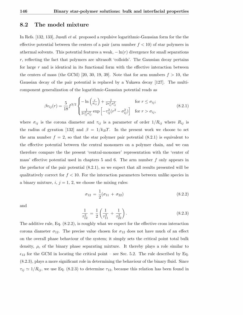
146 Binary star-polymer solutions: bulk and interfacial properties
8.2 The model mixture
In Refs. [132, 133], Jusufi et al. proposed a repulsive logarithmic-Gaussian form for the the
effective potential between the centers of a pair (arm number f < 10) of star polymers in
athermal solvents. This potential features a weak, − ln(r) divergence for small separations
r, reflecting the fact that polymers are ultrasoft ‘colloids’. The Gaussian decay pertains
for large r and is identical in its functional form with the effective interaction between
the centers of mass (the GCM) [20, 30, 19, 39]. Note that for arm numbers f > 10, the
Gaussian decay of the pair potential is replaced by a Yukawa decay [127]. The multi-
component generalization of the logarithmic-Gaussian potential reads as
βvij(r) =5
18f3/2
− ln(
rσij
)
+ 12τ2
ijσ2ij
for r ≤ σij ;
12τ2
ijσ2ij
exp[
−τ2ij(r
2 − σ2ij)
]
for r > σij ,(8.2.1)
where σij is the corona diameter and τij is a parameter of order 1/Rij where Rij is
the radius of gyration [132] and β = 1/kBT . In the present work we choose to set
the arm number f = 2, so that the star polymer pair potential (8.2.1) is equivalent to
the effective potential between the central monomers on a polymer chain, and we can
therefore compare the the present ‘central-monomer’ representation with the ‘center of
mass’ effective potential used in chapters 5 and 6. The arm number f only appears in
the prefactor of the pair potential (8.2.1), so we expect that all results presented will be
qualitatively correct for f < 10. For the interaction parameters between unlike species in
a binary mixture, i, j = 1, 2, we choose the mixing rules:
σ12 =1
2(σ11 + σ22) (8.2.2)
and1
τ212
=1
2
(
1
τ211
+1
τ222
)
. (8.2.3)
The additive rule, Eq. (8.2.2), is roughly what we expect for the effective cross interaction
corona diameter σ12. The precise value chosen for σ12 does not have much of an effect
on the overall phase behaviour of the system; it simply sets the critical point total bulk
density, ρc of the binary phase separating mixture. It thereby plays a role similar to
ε12 for the GCM in locating the critical point – see Sec. 5.2. The rule described by Eq.
(8.2.3), plays a more significant role in determining the behaviour of the binary fluid. Since
τij ' 1/Rij , we use Eq. (8.2.3) to determine τ12, because this relation has been found in

8.3 Bulk structure and phase diagram 147
simulations when considering the effective interaction between the centers of mass of the
polymers [30, 39] – this procedure is equivalent to the mixing rule (5.2.14).
In order to make a comparison with our earlier work in chapters 5 and 6, we choose
σ22/σ11 = 0.665 which is equivalent to a binary mixture of polymers of polymerisation
ratio N1 : N2 = 2 : 1.1 In Ref. [132], it was found that τii = 1.03/σii gives excellent
agreement with simulation results and, in addition, it brings about the best agreement
for the second virial coefficient of polymer solutions. Using these ratios along with Eqs.
(8.2.2) and (8.2.3), the model mixture parameters are completely determined.
8.3 Bulk structure and phase diagram
We consider a system consisting of M1 long and M2 short chains enclosed in the volume
V . Accordingly, we define the partial densities ρi = Mi/V , i = 1, 2 of the components,
as well as the total density ρ = ρ1 + ρ2 and the concentration of the small component,
x = ρ2/ρ. Due to the athermal character of the solvent the effective interactions are purely
entropic, i.e., they scale linearly with kBT and the thermal energy is the only energy scale
of the problem, as is clear from Eq. (8.2.1). Thereby, the temperature drops out of the
problem as an irrelevant variable and the thermodynamic space of the system is spanned
by the partial densities or equivalently the pair (x, ρ).
In order to determine the bulk structure of the binary fluid we use the hypernetted
chain (HNC) closure for direct pair correlation function, cij(r), in terms of the pair corre-
lation function hij(r) = gij(r) − 1 in the Ornstein-Zernike equations (the two component
generalisation of Eq. (2.2.1) [1]), which for a multi-component fluid is (c.f. Eq. (2.2.3)):
cij(r) = −βvij(r) + hij(r) − ln[1 + hij(r)]. (8.3.1)
We expect the HNC to be almost exact for describing the bulk structure of these soft
core particles at densities where the cores of the particles start to overlap (ρσ3 & 1.0).
This expectation is corroborated on the one hand from the known fact that for the one
component GCM the HNC results are indistinguishable from the simulation results at
these densities – see Ch. 4 and Refs. [22, 37, 38, 39] and on the other hand by the finding
that the HNC at high densities exhibits excellent agreement with simulation for a pure
1Recall that this arises from the scaling law R ∼ N ν connecting the spatial extent R of a self avoiding
polymer with its degree of polymerisation N , using the value ν = 3/5 for the Flory exponent.

148 Binary star-polymer solutions: bulk and interfacial properties
star-polymer fluid with functionality f = 32 [131].2
We define the partial structure factors Sij(k), i, j = 1, 2 of the mixture as
S11(k) = 1 + ρ1h11(k);
S22(k) = 1 + ρ2h22(k);
S12(k) =√
ρ1ρ2h12(k), (8.3.2)
where hij(k) denotes the Fourier transform of hij(r). In addition, we consider later the
concentration-concentration structure factor Scc(k), given by [134, 135]
Scc(k) = (1 − x)2S11(k) + x2S22(k) − 2x(1 − x)S12(k). (8.3.3)
In Fig. 8.1 we show the HNC partial structure factors for the binary fluid, comparing
also with the much simpler random phase approximation (RPA), which is given by cij(r) =
−βvij(r). The RPA closure to the Ornstein-Zernike equations becomes more accurate
as the density is increased and is very reliable for interaction potentials that diverge
slowly at the origin or are bounded there [38, 136]. Indeed, the RPA is in principle a
good candidate for examining the structure of uniform and nonuniform fluids, when the
condition∫
d3r vij(r) < ∞ is fulfilled [136, 129] – as is the case for the GCM one- and
two-component systems. For non-bounded but slowly diverging interactions, the RPA is a
good approximation at least for the thermodynamics, but it can also hold for the structure
when the prefactor of the weakly diverging potential is small [136]. For the case at hand,
the prefactor of the logarithmically diverging potentials is indeed small, (5/18)f 3/2 = 0.786
for f = 2, and thus the RPA should be valid at sufficiently high densities; a hypothesis we
confirm.
The comparison in Fig. 8.1 reveals that the HNC and the RPA yield very similar
structure factors. The discrepancies between the two occur mostly for small k-values and
are most pronounced in the neighbourhood of the critical point. The existence of a spinodal
(and thus of phase separation) in the mixture is witnessed in both the HNC and the RPA
by the increase (and eventual divergence) of the structure factors at k = 0. As we move
along a path of fixed concentration x increasing the total density ρ, the RPA-structure
factors are seen to diverge earlier than the HNC-ones, a feature pointing to the fact that the
2Due to the f3/2-prefactor of the star-star potential, the f = 32-effective interaction is much steeper
than the f = 2-one. The success of the HNC for this steeper interaction, then, guarantees its validity for
the much softer interaction considered here.

8.3 Bulk structure and phase diagram 149
0 1 2 3 4 5 6 7 8kσ11
0
1
2
3
4
S 11(k
)
HNC RPA
x = 0.0
x = 0.9
x = 0.5
x = 0.7
x = 0.3
(a)
0 1 2 3 4 5 6 7 8kσ11
0
1
2
3
4
5
S 22(k
)
HNC RPA
x = 0.7
x = 0.5
x = 0.3
x = 0.9
(b)x = 1.0
0 1 2 3 4 5 6 7 8kσ11
0.6
0.8
1.0
1.2
1.4
1.6
S 11(k
)
HNC RPA
0 2 4 6 80.5
1
1.5
2
2.5
3
3.5
ρσ11
3 = 5
(c)
0 1 2 3 4 5 6 7 8kσ11
0.4
0.6
0.8
1.0
1.2
1.4
1.6
1.8
2.0
S 22(k
)
HNC RPA
0 2 4 6 80
1
2
3
4
5
ρσ11
3 = 5
(d)
Figure 8.1: The partial structure factors, calculated along two different thermodynamic
paths in the (x, ρ)-plane of the star polymer mixture obtained from the HNC (solid lines)
and RPA (broken lines). (a) S11(k) for fixed total density ρσ311 = 5 and for different
concentrations x of species 2, as indicated on the plot. (b) Results for S22(k) along the
same path. (c) S11(k) at fixed concentration x = 0.7 and for increasing total densities,
from bottom to top ρσ311 = 1, 2, 3 and 4. The inset shows the result for ρσ3
11 = 5, a point
lying close to the RPA-critical (consolute) point (xc, ρcσ311) = (0.7095, 5.71628), see also
Fig. 8.3. The inset axes have the same labels as those of the main plot. (d) Same as in
(c) but for the partial structure factor S22(k). Note that in all plots the k → 0-limits
predicted by the RPA are larger than those from the HNC and the discrepancies become
more pronounced in the neighbourhood of the RPA-critical point. At the critical point
S11(k = 0) and S22(k = 0) → +∞ whereas S12(k = 0) → −∞.

150 Binary star-polymer solutions: bulk and interfacial properties
RPA-coexistence region will be broader than the one predicted by the HNC. In addition,
the fluid structure factors are quite similar to the equivalent GCM partial structure factors
Sij(k). The reason for this is that in calculating Sij(k) one Fourier transforms the pair
potentials, vij(r), which involves integrals of the form∫
dr r sin(kr)vij(r). Therefore,
the weak divergence of the pair potential vij(r) at small r has little effect because it is
suppressed by the multiplication with r sin(kr). It is rather the fashion in which vij(r)
decays as r → ∞ that has greater influence on the structure and the thermodynamics of
the mixture [20, 137]: as we show later, the quantity vij(0) ∝∫
dr r2vij(r) enters into the
RPA equation of state and is thus decisive in determining the phase boundaries.
We now turn our attention to the partial radial distribution functions (rdf’s) gij(r),
i, j = 1, 2, in particular at high densities and close to the borderlines x = 0 and x = 1.
In these cases, the HNC and the RPA yield practically identical results, so we examine
the HNC results here. As shown in Fig. 8.2, we find a signature of ‘clustering’ in the
rdf’s gij(r) of the minority phase, i.e., the development of a pronounced maximum. This
feature was also found for the GCM, e.g. see Fig. 7.13 and Ref. [47], but there the maxima
are at r = 0. In the present model gij(r) does not have a maximum at r = 0, because
our potentials have the logarithmic divergence at r = 0. Rather, the minority phase rdf’s
gii(r), have a peak in the range σii/2 . r . σii. Since σii is the diameter of the i-species
and r denotes distances between the central monomers, this corresponds, roughly, to the
centers of mass accumulating in one region and the polymers in the minority phase building
clusters. There is therefore good agreement between the center-of-mass and the central
monomer representation. Moreover, this clustering effect, which is more pronounced for
the large polymers, is an additional signature of phase separation.
Next we consider the overall phase behaviour of the mixture and make a comparison
between the binodal obtained from the HNC equation of state and that obtained from the
particularly simple RPA equation of state. The simplest (RPA) mean-field Helmholtz free
energy functional for the mixture reads as
F [ρi] = Fid[ρi] +1
2
∑
ij
∫
d3r1
∫
d3r2 ρi(r1) ρj(r2)vij(|r1 − r2|) (8.3.4)
where Fid is the ideal gas part – recall from Ch. 5 that this functional generates the RPA
direct pair correlation functions
c(2)ij (r1, r2) = c
(2)ij (|r1 − r2|) = −βvij(|r1 − r2|). (8.3.5)

8.3 Bulk structure and phase diagram 151
0 1 2 3 4 5r/σ11
0.0
0.2
0.4
0.6
0.8
1.0
1.2
g 11(r
)
x = 0.90, ρσ11
3 = 6.0
x = 0.95, ρσ11
3 = 8.0
x = 0.98, ρσ11
3 = 10.0
x = 0.99, ρσ11
3 = 12.0
(a)
0 1 2 3r/σ22
0.0
0.2
0.4
0.6
0.8
1.0
1.2
g 22(r
)
x = 0.10, ρσ11
3 = 7.0
x = 0.05, ρσ11
3 = 8.0
x = 0.04, ρσ11
3 = 9.0
x = 0.02, ρσ11
3 = 10.0
(b)
Figure 8.2: The HNC radial distribution functions gii(r) of the minority phases at high
total densities. (a) Large particles, g11(r) and (b) small particles, g22(r).

152 Binary star-polymer solutions: bulk and interfacial properties
This functional (8.3.4) replaces all excess free energy contributions with the mean-field
interaction terms that are bilinear in the density profiles ρi(r) of the components. Such
an approximation is expected to be accurate for the system at hand, which is deprived
of hard cores and of significant short-range, excluded-volume correlations, in particular at
high densities when the particles interact with a very large number of ‘neighbours’. In the
bulk mixture the densities are constants, ρi(r) = ρi. Expressing these in terms of the total
density ρ and the composition variable x, we can write the bulk Helmholtz free energy per
particle f , as
f(ρ, x) = fid(ρ, x) +1
2ρ[(1 − x)2 v11(0) + 2x(1 − x) v12(0) + x2 v22(0)], (8.3.6)
which is equivalent to Eqs. (5.2.6) and (5.2.7). The ideal contribution, fid(ρ, x), contains
the ideal free energy of mixing, β−1x ln(x) + (1 − x) ln(1 − x) as well as an irrelevant
term with linear-ρ dependence. vij(0) is the q = 0 limit of the Fourier transform (FT) of
the pair potential:
vij(0) =
∫
d3r vij(r). (8.3.7)
Note that Eq. (8.3.6) is equivalent to calculating f from the compressibility route. We
Legendre transform to obtain the Gibbs free energy per particle g = f +Pv; where v = 1/ρ
is the volume per particle, and the pressure is given as P = −(∂f/∂v)x. The common
tangent construction on g yields the binodal (see also Ch. 5 Sec. 5.2) which is plotted
along with the spinodal in Fig. 8.3. We find that the binodal has a very similar shape
to that found for the GCM in Ch. 5, since they both have the same form for the bulk
Helmholtz free energy (8.3.6), but they differ in where they locate the critical point. For
the present star polymer model we find the critical point at ρcσ311 = 5.7 where the star
corona diameter σ11 ' 1.32Rg11, with Rg
11 the radius of gyration [132, 138]. On the other
hand, for the GCM studied in Ch. 5 we found ρcR311 = 5.6 with radius R11 ' Rg
11.
We also determined the HNC-phase diagram. The HNC closure breaks down before a
spinodal is reached, as is well-known from previous studies [139, 140]. However, this poses
no difficulties in calculating the HNC binodals.3 For all points in the region where the
HNC converges, we calculate the pressure P and partial chemical potentials µ1, µ2 on a
grid. For the HNC, this calculation is local, i.e., one needs no thermodynamic integration
3We found, in fact, that the locus of points on which the HNC fails to converge is a curve that runs
close to the RPA-spinodal and in the U-shaped region in the high-density part of this curve the HNC has
no solutions.

8.3 Bulk structure and phase diagram 153
0 0.1 0.2 0.3 0.4 0.5 0.6 0.7 0.8 0.9 1x
0
5
10
15
20
ρσ11
3
RPA−spinodal RPA−binodal HNC−binodal
(a)
0 0.1 0.2 0.3 0.4 0.5 0.6 0.7 0.8 0.9 1x
0
5
10
15
20
ρσ11
3
RPA−Spinodal RPA−Binodal Fisher−Widom line Lifshitz line for Scc(k) Lifshitz line for S11(k) Lifshitz line for S22(k)
A
B
C
D
E
F
G
(b)
MONOTONIC
OSCILLATORY
Figure 8.3: (a) The RPA-spinodal and binodal lines for the star-polymer mixture (dotted
and solid lines) along with the HNC-binodal (dashed line). x is the concentration of species
2, the smaller component. The straight segments denote HNC-tielines between coexisting
fluid phases whose coordinates are given by the closed circles at their ends. (b) The RPA-
phase diagram along with the Fisher-Widom line (light solid line) and the Lifshitz lines of
the various structure factors. The left hand branch of the FW line lies close to the Lifshitz
line for S11(k) (short dashed line) while the right hand branch lies close to the Lifshitz
line for S22(k) (long dashed line). The dash-dotted line is the Lifshitz line for Scc(k). The
points A-G on the right-hand branch of the binodal are located at total densities ρσ311 = 8,
10, 12, 14, 16, 18 and 20, at which the free interface density profiles will be calculated in
Section 8.4. The gray lines are RPA-isobars through the points A-G and their intersections
with the left-hand branch of the binodal yield the state points coexisting with A-G. The
open circle denotes the RPA-critical point.

154 Binary star-polymer solutions: bulk and interfacial properties
to obtain µ1 and µ2 [47, 141], since within the HNC
βµi = ln(Λ3i ρi) +
∑
j
[
ρj
2
∫
drhij(r)[hij(r) − cij(r)] − ρj cij(0)
]
(8.3.8)
where hij(r) and cij(r) are the HNC total and direct pair correlation functions. From
µ1 and µ2, the Gibbs free energy per particle g = (1 − x)µ1 + xµ2 is readily obtainable.
We perform a 2d-interpolation of the pressure results to obtain P (x, ρ) as a function of
two variables for any x and ρ, and on this surface we determine the isobar curves P =
constant. We then draw the Gibbs free energy along the isobars to obtain gP (x), where
the subscript now denotes that P is fixed. For those pressures for which gP (x) is a convex
function of x, the system is in a single (mixed) state. For those for which it is not, the
common tangent construction determines the coexistence concentrations and densities.
The region in which the HNC has no solutions presents no difficulties. For the isobars
that intersect the borderline of this region, we simply have gP (x) with two ‘branches’ on
either side of the prohibited domain and we perform the common tangent construction on
those.
The HNC binodal is plotted in Fig. 8.3 along with the RPA one. It can be seen
that there is very good agreement between the two. The RPA-binodal is slightly broader
but the discrepancies become quickly suppressed in moving away from the critical point.
If one interprets the total density as an ‘inverse temperature’ and the concentration as a
‘density’ of a hypothetical one-component system, then the phase diagram can be regarded
as that corresponding to ‘liquid-gas’ coexistence. The RPA is then equivalent to the the
mean-field approximation, which usually delivers critical temperatures higher than the
true result. That the RPA critical density is lower than the HNC-one can be explained by
means of this analogy. The largest discrepancies between HNC and RPA occur close to
the critical point but these are less than 10% for the location of the binodal on the density
axis. Otherwise, the remarkable accuracy of the RPA can be understood by the fact that
the phase separation for our binary fluid occurs at a sufficiently high density that the
differences between the RPA and HNC routes to the bulk structure and thermodynamics
are indeed very small. We demonstrate this in Fig. 8.4, where we show representative
results for the chemical potentials and the pressure obtained by the two approaches. We
note that Finken et al. [47] have also made comparisons between the RPA and HNC
results for the binodal in the case of a binary mixture of repulsive GCM particles. They
report larger differences between the two theories than we find here. At present it is not

8.3 Bulk structure and phase diagram 155
clear why the differences should be larger for GCM particles than for the (very similar)
logarithmic-Gauss potentials we consider in the present study.
More detailed information about the nature of the interparticle correlations in the
mixture can be obtained by investigating the Fisher-Widom (FW) line [2]. The FW line
is determined by the asymptotic decay, r → ∞, of the total pairwise correlation functions
hij(r). It is the locus of points in the phase diagram, at which the ultimate decay of the
pair correlation functions crosses over from monotonic (Ornstein-Zernike like) to damped
oscillatory. The method for determining the FW line in mixtures is described in Ch. 5
Sec. 5.4, see also Ref. [52]. Using the RPA approximation for the direct pair correlation
function, cij(q) = −βvij(q), greatly facilitates the calculation of the FW-line (as it did
for the GCM), since the Fourier transforms vij(q) are analytic (see Appendix E). The
FW line for the present mixture is displayed in Fig. 8.3. We find that FW line is almost
exactly the same in shape and location in the phase diagram as that found, also using
the RPA, for the binary GCM corresponding to a 2:1 length ratio mixture of polymers –
see Fig. 5.1. We also find the same cusp in the FW line (bottom right hand corner, Fig.
8.3(b)) and the new line found for the GCM in Ch. 5. The latter denotes the crossover
from oscillatory decay with one wavelength, corresponding to the length-scale associated
with one of the particle species, to oscillatory decay with another wavelength, determined
by the size of the other species of particles. Because the RPA binodal and FW lines are
so similar in the present model to those found for the binary GCM in Ch. 5, we expect
the trends found as particle size asymmetry was varied in the GCM, to carry over to the
present model, i.e., as the size asymmetry is increased, the location of the critical point
should move towards the side of the phase diagram rich in the smaller species and the
cusp in the FW line should move to this side also. Note also that the pole determining
the asymptotic decay of gij(r) also sets the common bulk correlation length: ξ = 1/α0
[52]. It is possible to calculate the leading pole from numerical solutions of the HNC [57],
however we expect the asymptotic decay to be very well captured by the RPA, and the
dominant HNC pole to be very similar in value to that obtained from the analytically
tractable RPA, as was the case for the one-component GCM,4 – see Fig. 5.12.
The Lifshitz line [142, 143]5 separates the region in the phase diagram in which Sij(k)
4L.R. Croft, private communication.5We note that for microemulsions both the Lifshitz- and the FW-line are used to signify the crossover
from the ‘sponge phase’ to the ‘random phase’ (there is no sharp thermodynamic transition between

156 Binary star-polymer solutions: bulk and interfacial properties
0 1 2 3 4 5 6ρσ11
3 −10
−5
0
5
10
15
20
25
30
βµ1,
βµ 2
βµ1 (HNC)βµ2 (HNC)βµ1 (RPA)βµ2 (RPA)
(a)
0 1 2 3 4 5 6ρσ11
3 0
10
20
30
40
50
60
70
βPσ 11
3
HNC RPA
(b)
Figure 8.4: Comparison of the HNC- and RPA-results for the partial chemical potentials
(a) and the total pressure (b), at fixed concentration x = 0.5 and increasing total density
ρ.

8.4 The free fluid-fluid interface 157
has a local maximum at k = 0 (as occurs near a critical point or spinodal) from that
in which it has a local minimum at k = 0. Making a small k expansion of the partial
structure factors
Sij(k) = a(ρ, x) + b(ρ, x)k2 + O(k4), (8.3.9)
and examining the sign of the term b(ρ, x), one sees that the Lifshitz line is the locus of
points b(ρ, x) = 0. The Lifshitz lines for two of the partial structure factors are displayed
in Fig. 8.3 and their shapes are similar to branches of the FW-line. This is because their
locations are driven by the proximity of the spinodal, which forces S11(k) and S22(k) to
have maxima at k = 0. These maxima survive as long as the pure imaginary pole (away
from the spinodal) is the dominant one. Close to the crossover to damped oscillatory
decay in hij(r), at the FW line, the maximum turns into a minimum. Hence the Lifshitz
and the FW-lines are closely related to one another but they are not identical. Since
phase separation in liquid mixtures is driven by concentration fluctuations it is natural
to examine the Lifshitz line for the concentration-concentration structure factor Scc(k)
defined in Eq. (8.3.3). As can be seen in Fig. 8.3, the domain enclosed by the Lifshitz line,
in which Scc(k = 0) is a maximum, is broader than the domain in which both S11(k = 0)
and S22(k = 0) are local maxima. This is the effect of the term −2x(1−x)S12(k). In fact,
the Lifshitz line for Scc(k = 0) does not close: even at very low densities, there survives a
domain, in this case 0.55 . x . 0.77, in which Scc(k) has a small maximum at k = 0. The
Lifshitz line for S12(k) runs similarly to the one for S11(k), but the regions it separates
are inverted with respect to the ones for S11(k) and S22(k): above the Lifshitz line for
S12(k), the latter has a local minimum at k = 0 and below it a local maximum,6 whereas
the situation is inverted for the other two.
8.4 The free fluid-fluid interface
In this section we calculate the inhomogeneous one-body density profiles of the fluid at
the planar interface between two coexisting phase-separated liquid phases and the corre-
the two, hence one resorts to structural criteria) [142, 143]. The locations of the two lines in the phase
diagram are related, as in the present fluid. We note also that in the microemulsion literature the FW-line
is referred to as the disorder line [142], the latter terminology being the common one for Ising models
[144, 145, 146, 49].6Note that at the spinodal S12(k = 0) diverges to minus infinity, not to plus infinity as do S11(k = 0)
and S22(k = 0).

158 Binary star-polymer solutions: bulk and interfacial properties
sponding surface tension γ, using the same DFT (8.3.4) which generates the RPA. Once
again we work with the grand potential functional
ΩV [ρi] = F [ρi] −∑
i
∫
d3r(µi − Vi(r))ρi(r), (8.4.1)
where µi is the chemical potential of species i = 1, 2, and determine the free interface
density profiles by setting the external potentials Vi(r) = Vi(z) = 0. Recall from Ch. 5.3
that within the present mean field approach the resulting profiles ρi(z), with z normal to
the interface, are non trivial, i.e., the interface has a finite width. Minimising (8.4.1) and
using (8.3.4) for F [ρi] yields a pair of coupled Euler-Lagrange equations for the profiles.
Due to the planar symmetry these can be reduced to a pair of 1-dimensional equations:
µi − Vi(z) = µi,id(ρi(z)) +∑
j
∫
dz′ρj(z′)vij(|z − z′|), for i, j = 1, 2 (8.4.2)
where the ideal gas chemical potential µi,id(ρi) = β−1 ln(Λ3i ρi) (Λi is the thermal de-Broglie
wave-length) and
vij(|z − z′|) =
∫ ∞
−∞dx
∫ ∞
−∞dy vij(|r − r′|). (8.4.3)
Eqs. (8.4.2) can be solved self consistently for the density profiles of the two species.
We find results very similar to those for the binary GCM in Ch. 5; again, the weak
divergence of the pair potential vij(r) has little effect. When (8.2.1) is substituted into
(8.4.3) we find that vij(z) is finite for all z: on integrating over the x − y plane the
− ln(r) divergence in vij(r) yields a term ∼ z2 ln(z), which is finite as z → 0. In fact
vij(z) resulting from Eqs. (8.2.1) and (8.4.3) has a very similar shape to that resulting
from substituting vij(r) = εij exp(−r2/R2ij) (GCM) into (8.4.3). The resulting density
profiles for the coexisting states marked in Fig. 8.3(b) are displayed in Fig. 8.5. We find
pronounced oscillations in the density profile of the larger species, ρ1(z), for states well
removed from the critical point, similar to those we found for the GCM in Ch. 5. For
states B-G (see the phase diagram Fig. 8.3) both density profiles ρ1(z) and ρ2(z) exhibit
non-monotonic decay into the bulk phase which is rich in species 1. On the other side of
the interface, approaching the bulk phase rich in species 2, magnification shows that both
ρ1(z) and ρ2(z) are non-monotonic for states E-G. For state A, closer to the critical point,
there is no sign of oscillations on either side of the interface.
As with the GCM, it seems to be the location of the FW line that determines the
crossover from monotonic to damped oscillatory decay in the free interface density profiles.
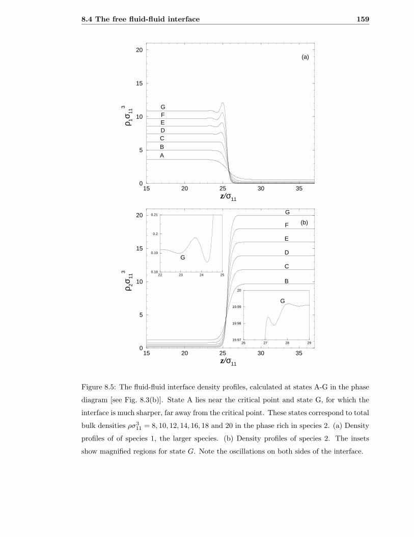
8.4 The free fluid-fluid interface 159
15 20 25 30 35z/σ11
0
5
10
15
20
ρ 1σ11
3
ABCDEFG
(a)
15 20 25 30 35z/σ11
0
5
10
15
20
ρ 2σ11
3
22 23 24 250.18
0.19
0.2
0.21
26 27 28 2919.97
19.98
19.99
20
B
C
D
E
F
G
G
G
(b)
Figure 8.5: The fluid-fluid interface density profiles, calculated at states A-G in the phase
diagram [see Fig. 8.3(b)]. State A lies near the critical point and state G, for which the
interface is much sharper, far away from the critical point. These states correspond to total
bulk densities ρσ311 = 8, 10, 12, 14, 16, 18 and 20 in the phase rich in species 2. (a) Density
profiles of of species 1, the larger species. (b) Density profiles of species 2. The insets
show magnified regions for state G. Note the oscillations on both sides of the interface.

160 Binary star-polymer solutions: bulk and interfacial properties
On moving along the binodal away from the critical point, and crossing the intersection
with the FW line, there are bulk states (on the binodal) at which the the pair correlation
functions, hij(r), decay in a damped oscillatory fashion. Since it is the same pole in the
structure factors that determines the asymptotic decay of the one-body density profiles,
ρi(r), for these states on the oscillatory side of the FW line one should expect damped
oscillatory decay of ρi(r) into the bulk phase. For the present model the FW line intersects
the binodal on both sides so that when both bulk coexisting states are on the oscillatory
side of the FW line, then the asymptotic decay of the density profiles will be damped
oscillatory on both sides of the interface – as we found in Ch. 5 for the binary GCM.
Having calculated the equilibrium free interface density profiles we can determine the
surface tension, which is defined as the excess grand potential per unit area and can be
written as
γ =
∫ ∞
−∞dz (P + ω(z)) , (8.4.4)
where P is the bulk pressure at coexistence and ω(z) is the grand potential density obtained
from Eqs. (8.3.4) and (8.4.1) with Vi(z) = 0. The reduced tension γ∗ = βγσ211 is plotted in
Fig. 8.6 for the interfaces corresponding to Fig. 8.5. We have chosen to plot γ∗ versus the
order parameter (ρA1 − ρB
1 )σ311, where ρA
1 is the bulk density of species 1 in phase A, rich
in species 1, and ρB1 is the same quantity in phase B, poor in species 1 – as we did for the
binary GCM in Ch. 5. Mean-field arguments imply that γ∗ should vanish as (ρA1 − ρB
1 )3
on approaching the critical point and this is confirmed by our numerical results (see inset
to Fig. 8.6).
We can obtain an estimate for the surface tension of a phase separated mixture of ‘real’
star-polymers by choosing γ∗ = 5, corresponding to a state well removed from the critical
point, and setting T = 300 K and σ11 = 20 nm. We find γ = 52 µN/m, the same as for the
GCM.
The numerical values of γ∗ determine whether we can expect to observe oscillatory
density profiles in a more accurate treatment of the free interface. As the present mean
field functional does not include the effects of capillary wave fluctuations one needs to
make an estimate of these fluctuation effects on oscillatory structure [7]. In Ch. 5 on
the GCM free interface we addressed the issue of whether capillary-wave fluctuations
would destroy the layering structures we found in the DFT treatment of the interface.
The situation for the present model is the same as for the GCM; i.e., we assume that
DFT describes the ‘bare’ or ‘intrinsic’ profiles – which might be oscillatory, as in the

8.4 The free fluid-fluid interface 161
100
10110
−3
10−2
10−1
100
101
102
0 1 2 3 4 5 6 7 8 9 10 11
(ρ1
A−ρ1
Β)σ11
3
0
1
2
3
4
5
6
7
8
9
10
11
12
13
14
15
βγσ 11
2
Figure 8.6: The reduced surface tension, γ∗ = βγσ211, at the planar free interface, plotted
against the order parameter (ρA1 − ρB
1 )σ311, the density difference in species 1 between the
two phases, which vanishes at the critical point. The line joining the data points is a
guide to the eye. Inset: double-logarithmic plot of the same quantities, demonstrating the
power-law dependence of γ∗; the straight line has gradient 3.
present case – and that fluctuations can be unfrozen on these. If one performs a Gaussian
smearing of the profiles over the interfacial thermal roughness ξ⊥ for a density profile
with decaying oscillations of wavelength 2π/α1 and decay length α−10 , these quantities
are unaltered but the amplitude is reduced by a factor exp[−(α21 − α2
0)ξ2⊥/2] [52, 61]. The
roughness ξ⊥ depends on the interfacial area L2x and on the external potential, e.g. gravity.
Ignoring the latter one finds that the amplitude of the oscillations in the density profile
should be reduced by a factor (Lx/ξ)−ω[(α1/α0)2−1] where ω ≡ (4πβγξ2)−1 is, as usual,
the dimensionless parameter which measures the strength of capillary wave fluctuations
and ξ ≡ (α0)−1. The larger the value of ω ∝ 1/γ∗, the more damped are the oscillations.
As mentioned in Ch. 5.5 the power law dependence on the interfacial area L2x that this
unfreezing procedure predicts is supported by the simulations of Toxvaerd and Stecki
[62] and those of Chacon et al. [58, 59, 60]. For the present model at states where the
oscillations in the DFT profiles are very pronounced, as with the GCM, the calculated

162 Binary star-polymer solutions: bulk and interfacial properties
exponent in the power law is small, typically −0.1, which implies that the the amplitude
of the oscillations at these particularly ‘stiff’ interfaces should only be weakly damped
by the capillary-wave fluctuations. As emphasized in Ch. 5 the reduced surface tension
γ∗ far from the critical point is very large in these liquid mixtures since the coexisting
phases correspond to a very high pressure and there are very large density differences,
for the individual species, between the phases – see Fig. 8.3. Such large values of γ∗ do
not normally arise at the liquid-vapour interface of simple, one-component fluids where
the solid phase intervenes at low temperatures. However the model considered by Chacon
et al. [58, 59, 60] ensures that the ratio of the melting temperature Tm to the critical
temperature Tc is small, i.e., Tm/Tc . 0.2, and in these circumstances γ∗ can be large and
then damping of the oscillations is weak.
8.5 Star-polymers at a hard wall: wetting behaviour
By integrating the normal component of the osmotic pressure in the interior of the star
polymer along the area of contact between the star and the wall, Jusufi et al. [132] were able
to calculate the force, F (z), and therefore the potential acting between a star-polymer and
a hard wall, with z denoting the distance from the star center to the planar wall surface.
The force scales as F (z) ∼ 1/z as z → 0, and for z → ∞ the form F (z) ∼ (∂/∂z)erf(κiz)
pertains, where erf(x) = (2/√
π)∫ x0 dt exp(−t2) is the error function and κ−1
i is a length
scale of order the radius of gyration of the polymer. For a star polymer with f = 2,
the value κi = 1.16/σii was found to give the best fit to simulations [132]. By matching
these two forms at z = σii/2 and then integrating to get the potential, Jusufi et al. [132]
proposed the following form for the effective potential Vi(z) between a star polymer and
a hard, planar wall:
βVi(z) = Λf3/2
− ln(
2zσii
)
−(
4z2
σ2ii− 1
)
(
ψi − 12
)
+ ζi for z ≤ σii/2;
ζierfc(κiz)/erfc(κiσii/2) for z > σii/2(8.5.1)
where erfc(x) = 1 − erf(x) is the complementary error function, ψi = (1 + κ2i σ
2ii/2)−1 is a
parameter chosen to guarantee the continuity of the local osmotic pressure in the interior
of the star polymer and
ζi =2√
πψi
κiσiierfc
(κiσii
2
)
exp
(
κ2i σ
2ii
4
)
. (8.5.2)

8.5 Star-polymers at a hard wall: wetting behaviour 163
0 2 4 6 8 10 12 14 16z/σ11
0
2
4
6
8
10
12
14
16
ρ 1σ11
30 2 4 6 8 10 12 14 16
z/σ1
0
2
4
6
8
10
12
14
16
ρ 2σ11
3
Figure 8.7: The density profiles of species 1, the larger particles, adsorbed at a wall
described by the potential (8.5.1), calculated along a path of constant total density, ρσ311 =
7.0, i.e., path A in Fig. 8.8. From left to right the profiles refer to x = 0.99, 0.95, 0.9,
0.88, 0.879, 0.878955, 0.878951 and 0.8789505, where x is the concentration of species 2
and xcoex = 0.87895019. The thickness of the adsorbed film increases continuously as
x → x+coex, indicating complete wetting. The inset shows the density profiles of species 2
for the same values of x. Note that species 2 is depleted from the region adjoining the
wall.
The final parameter Λ, which has a weak f dependence, is also chosen to match the
simulation results, giving Λ = 0.46 when f = 2 [132].
By using Eq. (8.5.1) for the external potential in Eq. (8.4.1) we are modeling the binary
star polymer fluid at a hard wall. We found that for certain states approaching the binodal
on the side poor in species 1, the larger particles, a thick wetting layer of the coexisting
phase rich in species 1 was adsorbed at the wall, the thickness of which diverged at the
binodal. Typical wetting density profiles are displayed in Fig. 8.7. These were calculated
along a constant density path ρσ311 = 7.0, approaching the binodal (path A in Fig. 8.8).
Upon investigating higher total densities we found there is a first order wetting transition,
above which the wall no longer wets completely. The point on the binodal at which the

164 Binary star-polymer solutions: bulk and interfacial properties
0 0.1 0.2 0.3 0.4 0.5 0.6 0.7 0.8 0.9 1x
0
5
10
15
20
ρσ11
3
0.95 0.955 0.96x
8.7
8.8
8.9
9
9.1
9.2
ρσ11
3
Spinodal
Binodal
pre−wettingline
A
Binodal
Figure 8.8: The phase diagram obtained from the RPA (as in Fig. 8.3). The two filled
circles show the location of the pre-wetting line. The upper point on the binodal is the
wetting point where the pre-wetting line meets the binodal tangentially and the lower
point is the critical point at the end of the pre-wetting line. The inset shows the pre-
wetting line at greater magnification. The horizontal path labeled A is that along which
the density profiles in Fig. 8.7 are calculated.
wetting transition occurs, the wetting point, is at (x, ρσ311) = (0.959, 9.15). Descending
from the wetting point is a short pre-wetting line, ending in a pre-wetting critical point
at (x, ρσ311) = (0.951, 8.75). The pre-wetting line is displayed in Fig. 8.8. This wetting
scenario is very similar to that which we found in Ch. 6 for the binary GCM fluid at a
planar wall with a repulsive Yukawa potential mimicking the effective potential between
the Gaussian particles and a hard wall.
The wetting point and the pre-wetting line were determined by analysing the density
profiles and the adsorption of species 1, Γ1, defined by
Γ1 =
∫ ∞
0dz (ρ1(z) − ρ1), (8.5.3)
where ρ1 = ρ1(∞), the density of species 1 in the bulk, i.e., far away from the wall. At the
pre-wetting line, the adsorption exhibits a discontinuous jump. In Fig. 8.9, the adsorption
calculated along constant total density paths (ρσ311 = 9.0, 8.9, 8.8 and 8.7) approaching

8.5 Star-polymers at a hard wall: wetting behaviour 165
the binodal is plotted. Figs. 8.9(a)-(c) correspond to paths that intersect the pre-wetting
line, whereas the path of Fig. 8.9(d) passes just below the pre-wetting line critical point.
We determine the location of the pre-wetting line by monitoring the jump in Γ1 and, in
the region of the pre-wetting critical point, the erosion of two branches in the free energy.
On solving numerically for the density profiles, one moves first along one branch, and
then jumps to the other before converging to the equilibrium solution. Note also that the
interfacial compressibility, χ12 = ∂Γ1/∂µ2 ∝ (∂Γ1/∂x)ρ still has a pronounced peak below
the critical point – see Fig. 8.9(d). The jump in the adsorption decreases for intersecting
paths approaching the pre-wetting critical point. These results should be compared with
those of Fig. 8.10, where Γ1 is plotted along the ρσ311 = 7.0 path (path A in Fig. 8.8),
along which the density profiles in Fig. 8.7 are calculated. This path is far away from the
wetting transition, and the film thickness increases smoothly with no jumps as the binodal
is approached; the thickness eventually diverging at the binodal.
We find that in the limit x → x+coex, below the wetting point Γ1 increases linearly with
− ln ∆x, where ∆x = (x − xcoex) is the deviation from coexistence. This linear increase
with − ln ∆x is illustrated in Fig. 8.10. For ∆x → 0+, Γ1, as defined by (8.5.3), scales
proportionally to the film thickness l, i.e., Γ1 ∼ l(ρA1 −ρB
1 ), where ρA1 is the bulk coexisting
density of species 1 in phase A, rich in species 1 and wetting the wall, and ρB1 is the bulk
density in phase B, poor in species 1. Equivalent behaviour was found for the GCM in Ch.
6 where we were able to describe the results by considering an effective interface potential,
Eq. (6.3.1), of the form
ωex(l; x) = l(
ωA − ωB)
+ γw,A + γA,B + ae−l/ξw + O(e−2l/ξw), (8.5.4)
where γw,A is the surface tension of the wall-phase A interface, γA,B that of the free A-B
interface, a is a coefficient dependent on ρ and ξw is the bulk correlation length in the
phase wetting the wall [11, 69, 15]. Eq. (8.5.4) is valid for a complete wetting situation;
minimisation of ωex with respect to l yields the equilibrium film thickness l for a given
undersaturation ∆x. ωB is the grand potential per unit volume in bulk phase B at given
chemical potentials µ1 and µ2, while ωA is the corresponding quantity in phase A at the
same chemical potentials. To lowest order in the chemical potential deviations:
ωA − ωB ' (ρA1 − ρB
1 )∆µ1 + (ρA2 − ρB
2 )∆µ2. (8.5.5)
Since ∆µi ≡ (µi − µi,coex) ∝ ∆x to lowest order, it follows that the first term on the right
hand side of Eq. (8.5.4) is proportional to l∆x. Minimisation of Eq. (8.5.4) then yields

166 Binary star-polymer solutions: bulk and interfacial properties
−11 −9 −7 −5 −3ln(x−xcoex.)
0
5
10
15
20
25
−11 −9 −7 −5 −3
0
5
10
15
20
25
−11 −9 −7 −5 −3ln(x−xcoex.)
0
5
10
15
20
25
Γ 1σ11
2−11 −9 −7 −5 −3
0
5
10
15
20
25Γ 1σ
11
2
ρσ11
3=9.0 ρσ11
3=8.9
ρσ11
3=8.8 ρσ11
3=8.7
(a) (b)
(c) (d)
Figure 8.9: Plots of the adsorption of species 1, Γ1, versus the logarithm of the deviation
from bulk coexistence ln(x−xcoex), at constant total density ρ, for paths intersecting [(a)-
(c)] and passing just below (supercritical) (d) the pre-wetting line. The jumps in (a)-(c)
indicate the first-order pre-wetting transition.
l ∼ −ξw ln ∆x. We were able to confirm that the pre-factor to the logarithm is indeed
ξw = 1/α0, where α0 is the imaginary part of the pole with the smallest imaginary part
(see Sec. 8.3), in the structure factors, for the bulk wetting phase A.
The wall potential (8.5.1) that we employ decays as erfc(κiz) ∼ exp(−κ2i z
2)/√
πκiz
as z → ∞. If the wall potential we had chosen had a slower decay, then the effective
interface potential (8.5.4) might have additional wall contributions – see chapters 3 and
6, in particular Sec. 6.3.2.

8.6 Summary and concluding remarks 167
−16 −14 −12 −10 −8 −6 −4 −2ln(x−xcoex.)
0
5
10
15
20
25
30
Γ 1σ11
2
Figure 8.10: The adsorption of species 1, Γ1, along path A in Fig. 8.8 with constant
total density, ρσ311 = 7, as a function of the logarithm of the deviation from bulk coexis-
tence, ln(x − xcoex). The adsorption corresponds to the density profiles in Fig. 8.7. On
approaching the binodal, Γ1 increases linearly with − ln(x − xcoex).
8.6 Summary and concluding remarks
We have shown that a binary fluid of star-polymers, where the interactions between the
star-polymers are modeled by purely repulsive effective pair potentials, can phase separate
into two fluid phases. When the binodal lies at sufficiently high densities (ρσ311 & 5),
the quasi-exact HNC closure to the Ornstein-Zernike equations gives results for the bulk
structure and thermodynamics (including the binodal) which are very similar to those from
the much simpler RPA. We chose pair potential parameters to correspond to a binary fluid
of f = 2 arm star-polymers with length ratio 2:1 in order to compare with our results for
the binary GCM in Ch. 6. The GCM is an effective pair potential between the centers of
mass of polymer chains, so by choosing f = 2 the star-polymer pair potential should also be
that between the central monomers on a pair of polymers. We are therefore comparing two
perspectives: ‘central monomer’ versus ‘center of mass’ as the coordinate for the effective
pair potential between the polymers. Since it is the same underlying polymer system
that both are describing, the thermodynamics and, therefore, phase diagrams should be

168 Binary star-polymer solutions: bulk and interfacial properties
similar, and this is indeed what is found. Since the structure of the fluid is dependent on
the particular ‘perspective’ one takes for describing the fluid, one should expect somewhat
different structure factors and pair correlation functions. However, the two approaches
give a surprisingly similar picture in terms of the location of the FW line relative to
the binodal and the values for the bulk correlation length ξ. At this level it appears to
matter little that one approach employs an effective pair potential that is finite at r = 0
(the GCM) whereas the other has a weakly diverging pair potential (the star-polymer).
We also found the same line denoting the crossover in the asymptotic decay of the pair
correlation functions hij(r) from damped oscillatory decay with one wavelength to damped
oscillatory with another wavelength, joining the cusp in the FW line, that was found for
the GCM in Ch. 5.4. By calculating the Lifshitz lines we showed that the location of these
is closely related to that of the FW line.
Having shown that the RPA closure is a very good approximation for bulk pair correla-
tion functions, we used the simple Helmholtz free energy functional (8.3.4) which generates
the RPA to calculate one-body density profiles for the inhomogeneous fluid mixture. In
the case of the free fluid-fluid interface the density profiles of both species showed os-
cillations on both sides of the interface for certain states. The onset of the oscillations
was accounted for by the location of the FW line. We also calculated the density profiles
of the fluid at a repulsive wall potential equivalent to the effective potential between a
star-polymer and a hard wall, and showed that there was a first order wetting transition,
with the associated pre-wetting line. The picture that emerged from these studies of the
inhomogeneous fluid is very similar to that for the binary GCM.
Chapter 9
Final Remarks
To conclude we return to possible applications of the binary GCM and the log-Gauss
potentials used in Ch. 8 to describe mixtures of polymers. As mentioned in chapter 4,
the effective interaction between two identical isolated nonintersecting polymer chains,
averaged over the internal conformations, is well represented by a Gaussian whose width
R is of the same order as the radius of gyration and whose height is a few kBT . The
simulation study of Louis et al. [19, 20] showed that the Gaussian shape remains a good
approximation to the effective potential in dilute and semi-dilute solutions of self-avoiding
random walk (SAW) polymers and that the parameters ε and R do not vary strongly
with the concentration of the polymer: ε ' 2kBT . The same authors showed that the
Gaussian effective potential reproduces the structure and thermodynamic properties of
SAW polymer solutions over a wide concentration range. Such a procedure has great
appeal as the monomer degrees of freedom no longer appear; one treats the chains as ‘soft
colloids’ [19, 20]. Much less is established for mixtures of polymers; it is not known how
well the phase separation found for the GCM (using the RPA and the HNC [47]) accounts
for that which is observed at high concentration in mixtures of polymers with different
chain lengths1. Our results predict demixing phase separation in the semi-dilute regime, in
agreement with the results of Refs. [147, 148]. Phase separation is, of course, also observed
in polymer blends (melts). Given the predictions of rich interfacial behaviour that have
emerged from the present study of the GCM it would be worthwhile to pursue further
possible connections between demixing in polymer systems and in the GCM.
1In order to introduce phase separation it may be necessary to introduce explicit monomer-monomer
repulsion in the underlying polymer system (A.A. Louis, private communication).
169

170 Final Remarks
One could improve upon the state-independent pair potential approximation used here
which is most reliable for modeling polymers in dilute solutions (ρR3 < 1), and is only
approximately correct in the semi-dilute regime [34, 20]. In the semi-dilute regime we
could expect the GCM (and log-Gauss) pair potentials to acquire some additional density-
dependence in their parameters, mimicking the effects of many-body forces. Since we
have ignored any such dependence in this work, we expect our results to be only semi-
quantitatively correct for modeling polymer mixtures in the semi-dilute regime.
The rich bulk and interfacial phenomena displayed by the simple model presented in
this thesis show that the ‘colloidal approach’ of deriving effective pair potentials between
complex polymeric molecules can be very fruitful. Moreover, the remarkable success of
the simple and analytically tractable RPA in accounting for bulk correlation functions
and thermodynamic properties of the present log-Gauss and Gaussian model opens new
perspectives for the study of the properties of inhomogeneous mixtures of such ultrasoft-
particle fluids. Given the variety of ways that exist in colloidal science to externally
manipulate the conformations of chain-like molecules, we expect the RPA-approach to be
a tool whose applicability will be much wider than simply the system of chains in athermal
solvents presented here.
Although the (binary) GCM provides a simple, zeroth order model for polymers in solu-
tion, we believe the most appealing aspect of the model is that the simple RPA Helmholtz
free energy functional Eq. (5.2.2), seems to provide quite an accurate description of the
GCM fluid. It is the simplicity of the RPA that is useful: The GCM can be treated as a
‘test-bed’ for new theories in any of a variety of different aspects of liquid-state physics.
We are referring particularly to the results in Ch. 7, where we were able to use this sim-
ple model to test whether the effects of thick adsorbed wetting films are incorporated in
a general DFT method for calculating the solvent mediated potential between two large
particles dissolved in a solvent near to fluid-fluid coexistence. Thanks to the simplicity of
the model we were able to resolve which correlation effects were included in the theory,
and which were neglected, and, for example, to determine what factors determined the
depth of the SM potential. Had we used a more sophisticated functional, then we doubt
whether such a detailed analysis of the influence of thick adsorbed wetting films on the
SM potentials would have been possible.
Another use to which the GCM has been put, was to test the dynamical DFT proposed
by Marconi and Tarazona [149, 150]. Dzubiella and Likos [151] used the one-component

Final Remarks 171
GCM to test whether the dynamical DFT was able to describe a fluid confined in an exter-
nal potential that was suddenly changed (for example, the situation one might envisage if
there were a number of colloids confined in an optical tweezer). These authors compared
the results of dynamical DFT with those of Brownian Dynamics simulations. The signifi-
cance of the results of Dzubiella and Likos [151] was not in the specific properties of the
dynamics of the Gaussian particles, rather it was the ability to test the basic formalism
of the dynamical DFT using a simple model. We plan to use the binary GCM in a sim-
ilar way, in order to develop theories for the dynamics of binary fluids, for example, the
dynamics of phase separation for a fluid confined in an external potential. The (binary)
GCM can therefore be viewed as a useful ‘test-bed’ for testing new theories.
As a final remark we note that the binary Gaussian Core Model is very different from
the binary Gaussian Model introduced by Helfand and Stillinger [152] – see also Ref. [153].
In the latter v11(r) = v22(r) = 0 while the Mayer-f -function f12(r) ≡ exp(−βv12(r)) − 1
is a Gaussian. This model also exhibits fluid-fluid phase separation at high densities
[152, 153].

Appendix A
DFT and the Einstein Model
In this Appendix we begin by reminding the reader of the Classical Einstein model of a solid.
We subsequently attempt to treat the Einstein model within a DFT framework, and show
why this approach breaks down. Finally we make some, rather speculative, conclusions
about DFT theories for solids in general.
The Einstein model is perhaps the simplest model of a solid. In the Einstein model we
consider a set of N particles each labeled i with position ri, momentum pi and mass m.
Each particle is bound by a harmonic potential
vi(ri) = α(ri − Ri)2, (A.0.1)
where α is the binding strength parameter, which determines how tightly the particle is
bound to the lattice site for this particle at Ri. The Hamiltonian for the Einstein model
is
H =N
∑
i=1
[
p2i
2m+ vi(ri)
]
. (A.0.2)
Since this is just the Hamiltonian for a set of N independent harmonic oscillators, the
partition function for the system QN = QN1 , where Q1 is the partition function for a single
oscillator. The partition function is
QN = h−3N
∫
drN
∫
dpN exp(−βH). (A.0.3)
Note that this does not have a 1/N ! indistinguishability factor – each particle is bound to
a different lattice site, and so the particles are distinguishable. The integrals in (A.0.3)
are all Gaussian, and so we obtain:
QN = Λ−3N
(
βα
π
)−3N/2
, (A.0.4)
173

174 Appendix A. DFT and the Einstein Model
where
Λ =
√
2πβ~2
m(A.0.5)
is the thermal de Broglie wavelength. The Helmholtz free energy is therefore
FEin = −kBT ln QN =3
2NkBT ln
(
Λ2βα
π
)
. (A.0.6)
Note that this free energy does not reduce to the ideal gas Helmholtz free energy in the
limit α → 0. This is a manifestation of the fact that by considering each particle bound
to a particular lattice site from the outset, the particles are distinguishable, which is not
the case for the ideal gas, or any other fluid. The internal energy is simply 3NkBT , which
we can obtain via the equipartition theorem, and the pressure P = −(∂F/∂V )T = 0 for
the Einstein model, since the free energy (A.0.6) is independent of the volume V .
The (time averaged) density profile for a single particle in an external potential is
simply proportional to the Boltzmann factor of that potential, which in the present case
of a harmonic potential, gives us a Gaussian density profile. The total density distribution
profile for the particles in the Einstein solid is therefore a sum of Gaussian peaks, each
centered around the set of lattice sites Ri:
ρ(r) =N
∑
i=1
ρi(r) =N
∑
i=1
(
βα
π
)3/2
e−βα(r−Ri)2
, (A.0.7)
where ρi(r) is the density contribution from the ith particle which has a Gaussian density
distribution centered around Ri and the prefactor to the Gaussian is determined from the
normalization condition of one particle per lattice site. As a consistency check we can
use the density profiles (A.0.7) to calculate the contribution to the Helmholtz free energy,
from the external potentials (A.0.1):
〈V 〉 =N
∑
i=1
∫
drρi(r)vi(r)
= α
(
βα
π
)3/2 N∑
i=1
∫
dr (r − Ri)2e−βα(r−Ri)
2
=3
2NkBT, (A.0.8)
which is, of course, simply the result one would obtain by applying the equipartition
theorem for the potential energy degrees of freedom.
Having recalled the Einstein solid, we shall now consider the results from DFT for the
same system. The basic idea behind most attempts to construct a classical DFT for solids,

Appendix A. DFT and the Einstein Model 175
is that one can treat the solid as a (highly) inhomogeneous fluid and that one can apply
a DFT constructed for the fluid phase to treat the solid phase. In DFT’s for the solid
phase one often assumes the one-body density profile is of the form in Eq. (A.0.7) with
α, an inverse width parameter for the Gaussian peaks, treated as a variational parameter
to minimize the free energy. In classical DFT one considers the following Helmholtz free
energy functional:
F [ρ] = F [ρ] +
∫
drρ(r)V (r), (A.0.9)
where F [ρ] is the intrinsic Helmholtz free energy functional and V (r) is the external poten-
tial on the fluid. For the present Einstein system we cannot express the external potential
contribution to the Helmholtz free energy in this way because the external potential is
different for each particle – see Eq. (A.0.1) – in the Einstein model the ith particle sees
the ith potential well. This should alert us to the possibility that the present DFT ap-
proach may fail. However, for the present, we shall assume that the external potential
contribution to the Helmholtz free energy is 〈V 〉 = 32NkBT , i.e. that given by Eq. (A.0.8).
Returning to Eq. (A.0.9), the intrinsic Helmholtz free energy functional F [ρ] is nor-
mally split up as follows
F [ρ] = Fid[ρ] + Fex[ρ], (A.0.10)
where Fid[ρ] is the ideal gas contribution and Fex[ρ] is the excess part, which includes the
effects of any interactions that there are between the particles. The ideal gas contribution
to the intrinsic Helmholtz free energy functional is
Fid[ρ] = kBT
∫
drρ(r) [ln Λ3ρ(r) − 1]. (A.0.11)
We consider an ideal gas (i.e. Fex[ρ] = 0), with the external potential on the ith particle
given by Eq. (A.0.1) – i.e. corresponding to the Hamiltonian for the Einstein model, Eq.
(A.0.2). It appears reasonable to substitute Eq. (A.0.7) into Eq. (A.0.11), in order to
obtain the kinetic energy contribution to the Helmholtz free energy. If the parameter
α in the external potential is large, then the Gaussian peaks in the density profile, Eq.
(A.0.7), will be extremely narrow, and if we assume that the contribution from overlap
between Gaussian density peaks on neighbouring lattice sites in the integral obtained from
inserting Eq. (A.0.7) into (A.0.11) will be negligible, then one obtains:
F solidid =
3
2NkBT ln
(
Λ2βα
π
)
− 5
2NkBT. (A.0.12)
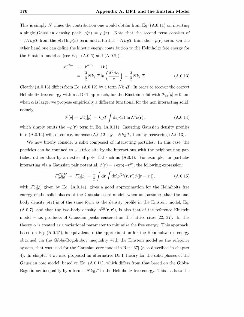
176 Appendix A. DFT and the Einstein Model
This is simply N times the contribution one would obtain from Eq. (A.0.11) on inserting
a single Gaussian density peak, ρ(r) = ρi(r). Note that the second term consists of
−32NkBT from the ρ(r) ln ρ(r) term and a further −NkBT from the −ρ(r) term. On the
other hand one can define the kinetic energy contribution to the Helmholtz free energy for
the Einstein model as (see Eqs. (A.0.6) and (A.0.8)):
FEinni ≡ FEin − 〈V 〉
=3
2NkBT ln
(
Λ2βα
π
)
− 3
2NkBT. (A.0.13)
Clearly (A.0.13) differs from Eq. (A.0.12) by a term NkBT . In order to recover the correct
Helmholtz free energy within a DFT approach, for the Einstein solid with Fex[ρ] = 0 and
when α is large, we propose empirically a different functional for the non interacting solid,
namely
F [ρ] = F∗ni[ρ] = kBT
∫
drρ(r) ln Λ3ρ(r), (A.0.14)
which simply omits the −ρ(r) term in Eq. (A.0.11). Inserting Gaussian density profiles
into (A.0.14) will, of course, increase (A.0.12) by +NkBT , thereby recovering (A.0.13).
We now briefly consider a solid composed of interacting particles. In this case, the
particles can be confined to a lattice site by the interactions with the neighbouring par-
ticles, rather than by an external potential such as (A.0.1). For example, for particles
interacting via a Gaussian pair potential, φ(r) = ε exp(−r2), the following expression:
FGCMsolid = F∗
ni[ρ] +1
2
∫
dr
∫
dr′ρ(2)(r, r′)φ(|r − r′|), (A.0.15)
with F∗ni[ρ] given by Eq. (A.0.14), gives a good approximation for the Helmholtz free
energy of the solid phases of the Gaussian core model, when one assumes that the one-
body density ρ(r) is of the same form as the density profile in the Einstein model, Eq.
(A.0.7), and that the two-body density, ρ(2)(r, r′), is also that of the reference Einstein
model – i.e. products of Gaussian peaks centered on the lattice sites [22, 37]. In this
theory α is treated as a variational parameter to minimize the free energy. This approach,
based on Eq. (A.0.15), is equivalent to the approximation for the Helmholtz free energy
obtained via the Gibbs-Bogoliubov inequality with the Einstein model as the reference
system, that was used for the Gaussian core model in Ref. [37] (also described in chapter
4). In chapter 4 we also proposed an alternative DFT theory for the solid phases of the
Gaussian core model, based on Eq. (A.0.11), which differs from that based on the Gibbs-
Bogoliubov inequality by a term −NkBT in the Helmholtz free energy. This leads to the

Appendix A. DFT and the Einstein Model 177
question, which is the better approximation for the Helmholtz free energy for the solid
phase? The first comment to make is that the free energy from the Gibbs-Bogoliubov
inequality provides an upper bound for the true free energy of the solid, however, the
DFT is constructed empirically, as is the case for many DFTs, on the basis that it gives
reasonable results for the phase behaviour of the GCM solid.
It is interesting to note that the extra −NkBT term in the Helmholtz free energy of the
solid does not change the value obtained for the pressure, P , of the solid. We demonstrate
this as follows: The Helmholtz free energy per particle, f = F/N = fni + fex, where fex is
the excess contribution for interacting particles and fni = FEinni /N is the non-interacting
part, can be written as (see Eq. (A.0.13)):
fni =3
2kBT ln α + (α independent terms). (A.0.16)
The pressure is thus
βP
ρ= βρ
∂f
∂ρ= βρ
∂fni
∂ρ+ βρ
∂fex
∂ρ
=3ρ
2α
(
∂α
∂ρ
)
+ βρf ′ex. (A.0.17)
For a given (ρ, T ), f is minimized with respect to α: ∂f/∂α|α=αmin = 0. Since the term
NkBT , which is the difference in the Helmholtz free energy obtained from the two theories,
is independent of α, this means that αmin is the same within both theories and therefore
(∂αmin/∂ρ) and the pressure P are the same within both theories. However, although
this term in the Helmholtz free energy does not change the pressure, it should affect the
values obtained for the chemical potential, and therefore any calculation of the liquid-solid
coexisting densities, as well as many other thermodynamic quantities for the solid phase;
for example, the extra term results in a difference of kB per particle (a significant amount)
in the value of the entropy calculated from the two theories for the Helmholtz free energy
of the solid phase. However, we do not believe these differences will significantly change
the phase diagram obtained for the GCM from these two theories.
Thinking beyond the GCM solid, we speculate, for certain model fluids, that it may
be profitable, when attempting to construct a DFT theory for the solid phase, to use Eq.
(A.0.14) as the non-interacting starting point for the theory, rather than Eq. (A.0.11). To
the expression in Eq. (A.0.14) one would then add an ‘excess’ functional F ∗ex[ρ], incorpo-
rating the contribution to the Helmholtz free energy arising from the interactions between
the particles.

178 Appendix A. DFT and the Einstein Model
We take the opportunity here to make a general point concerning the value obtained for
the entropy of the solid phase, when calculated within the DFT framework. We note that
DFT theories seem to systematically predict too low a value for the Lindemann ratio [46],
or equivalently, too large a value for the width parameter, α, for the Gaussian density peaks
– see Eq. (A.0.7). This can be seen in Baus’ review [45], where the Lindemann parameters
for some of the early theories of hard-sphere freezing are tabulated. It is also a feature
of the most recent theories for hard-sphere freezing, see for example Refs. [154, 46]. The
entropy of the solid depends quite sensitively on the value of α. The entropy change per
particle, ∆s = ∆S/N , on freezing has been calculated in several DFT theories of freezing
(see Ref. [45] and references therein), and there seems to be a discrepancy in the value
obtained for ∆s, when compared to simulations, that can be accounted for by considering
the discrepancy between the value obtained for α from DFT and from simulations: We
write the Helmholtz free energy as
f =3
2kBT ln α + Σ(T, α), (A.0.18)
where we have separated the α dependent part from the non-interacting part of the
Helmholtz free energy and we denote the remaining part by Σ(T, α). Σ(T, α) contains
both the (excess) contribution to the Helmholtz free energy, i.e. that due to the particle
interactions, as well as the α-independent terms in fid, the ideal-gas contribution to the
free energy. From Eq. (A.0.18) we can calculate the entropy per particle:
s = −(
∂f
∂T
)
ρ
= −3
2kB ln α − 3
2
kBT
α
(
∂α
∂T
)
ρ
−(
∂Σ(T, α)
∂T
)
ρ
. (A.0.19)
The entropy is therefore, of course, dependent on the parameter α, the inverse width
parameter for the Gaussian density peaks. We shall now turn to one of the more successful
applications of DFT to the problem of hard-sphere freezing, the theory of Curtin and
Ashcroft [155, 156]. In table A.1 we reproduce some of table I in Ref. [156] (see also
Ref. [45]), comparing liquid-solid coexistence data for the hard-sphere solid, from the
DFT theory and from simulations. ρs and ρl are the coexisting solid and liquid densities.
The Lindemann parameter L is related to the parameter α by L = (3/βαa2)1/2 and
a = (4/ρs)1/3 for the fcc lattice. Using these values we can determine the value of the
Gaussian width parameter α. From the simulation results, βαSIMσ2 = 77 and from the
DFT theory, βαDFT σ2 = 112, where σ is the hard-sphere diameter. Using these two
values we can calculate the difference in the non-interacting (ideal gas) part of the entropy

Appendix A. DFT and the Einstein Model 179
ρs ρl ∆s/kB L
Simulation 1.04 0.94 1.16 0.126
Theory 1.025 0.905 1.31 0.104
Table A.1: Liquid-solid coexistence data for the hard-sphere solid, reproduced from Ref.
[156]. ρs and ρl are the coexisting solid and liquid densities, L is the Lindemann parameter
and ∆s is the entropy change per particle on freezing.
in Eq. (A.0.19), 32kB ln(αDFT /αSIM ), from using these two different values for α (for
hard-spheres (∂α/∂T )ρ = 0, and therefore the second term in Eq. (A.0.19) is zero). This
difference is 32kB ln(112/77) = 0.56kB, which is clearly very substantial. Of course, in
calculating ∆s we must also consider the additional effect on the entropy of changing α in
the term Σ(T, α) in the Helmholtz free energy. Nevertheless, the difference, 0.56kB, from
the difference in α in the non-interacting part of the Helmholtz free energy does seem to
be important in accounting for the discrepancy in the entropy change on freezing. This
seems to suggest that to improve a DFT theory for freezing one should focus on generating
the correct value for α in the theory.


Appendix B
Details of the binary GCM Pole
Structure
In this Appendix we show some details of the pole structure for the binary GCM, which
gives rise to the new crossover line (analogous to the Fisher-Widom line) marking the cross-
over in the asymptotic decay of h(r) from damped oscillatory with a particular wavelength,
to damped oscillatory with a different wavelength. Such crossover occurs when there is
a large enough asymmetry in the sizes of the of the two different species of particles. In
Figs. B.1 and B.2, we show the imaginary and real parts of the poles respectively, plotted
versus x, the relative concentration of species 2, for a binary fluid of GCM particles with
total density ρR311 = 2.0 and ε12 = ε11 = ε22 = 2kBT . In both figures, plots a) – f) show
the trend as we change the size asymmetry, q = R22/R11, between the two species in the
binary fluid. In Fig. B.1, we see that the pole with the smallest α0 is one with α1 6= 0
for x ' 0, but as x is increased → 1, the curve for this pole intersects the curve for a
purely imaginary pole (dashed line) twice – these two intersections give rise to the two
branches of the Fisher-Widom line. For plots a) – d), in Fig. B.1, there is no crossover
between poles with different real parts, α1. However, for plots e) – f), the two (solid)
curves corresponding to the poles with the lowest values for α0, each with different values
of α1 6= 0, cross over. For x . 0.7, it is the branch of α1 which is smallest in magnitude
in Fig. B.2, which corresponds to the pole with the smallest value of α0 in Fig. B.1. For
plots e) – f), there is a crossover at x ' 0.7 from the pole with the smallest value of α0
and α1, to a different pole, for which α0 is the lowest in magnitude, but for which α1 has
the second lowest magnitude – i.e. for x & 0.7 there is a pole with a lower value for α1,
181

182 Appendix B. Details of the binary GCM Pole Structure
but a larger value for α0, than the pole which determines the asymptotic decay of h(r)
and which has the lowest value for α0. For this density the cross-over between the two
poles occurs in the region of the phase diagram where the purely imaginary pole dominates
the asymptotic decay of h(r), but at lower densities ρ, these poles have α0 with a value
lower than that for the purely imaginary pole, and therefore the asymptotic decay of h(r)
crosses over from damped oscillatory, to damped oscillatory with a different wavelength –
the locus of the cross over points in the phase diagram gives us the lines in the bottom
right hand corner of Figs. 5.1, 5.2 and 5.3.
0 0.5 1
0
2
4
6
α0R11
0 0.5 1 0 0.5 1
0
2
4
6
0 0.5 1x
0
2
4
6
α0R11
0 0.5 1x
0 0.5 1x
0
2
4
6
a) b) c)
d) e) f)
Figure B.1: Imaginary part of the poles, α0, plotted versus x, the relative concentration
of species 2, for a binary fluid of GCM particles with fixed total density ρR311 = 2.0 and
ε12 = ε11 = ε22 = 2kBT . The solid lines correspond to poles with a non-zero real part, and
the dashed line, to the purely imaginary pole. Plots a) – f) correspond to different size
asymmetries, q = R22/R11. In a), q = 0.75; in b) q = 0.72, in c) q = 0.71, in d) q = 0.707,
in e) q = 0.705 and in f) q = 0.7.
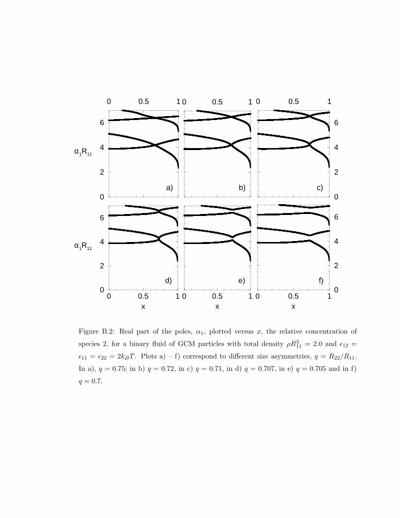
0 0.5 1
0
2
4
6
α1R11
0 0.5 1 0 0.5 1
0
2
4
6
0 0.5 1x
0
2
4
6
α1R11
0 0.5 1x
0 0.5 1x
0
2
4
6
a) b) c)
d) e) f)
Figure B.2: Real part of the poles, α1, plotted versus x, the relative concentration of
species 2, for a binary fluid of GCM particles with total density ρR311 = 2.0 and ε12 =
ε11 = ε22 = 2kBT . Plots a) – f) correspond to different size asymmetries, q = R22/R11.
In a), q = 0.75; in b) q = 0.72, in c) q = 0.71, in d) q = 0.707, in e) q = 0.705 and in f)
q = 0.7.


Appendix C
Derivation of Eq. (7.3.37) for the
excess chemical potential
Inserting Eq. (7.3.10) into Eq. (7.3.35) we obtain:
ω(r) = − 1
β
(
ρ0s − ρ∗e−r2/R2
bs
)
−1
2
(
ρ0s − ρ∗e−r2/R2
bs
)
(
ρ0s v
0ss − ρ∗π3/2εssR
3e− r2
R2ss
(
1− R2
R2ss
)
)
(C.0.1)
where R is given by Eq. (7.3.12). Subtracting Eq. (7.3.36) gives:
ω(r) − ω(∞) =1
βρ∗e−r2/R2
bs +1
2ρ0
sρ∗v0
sse−r2/R2
bs +1
2ρ0
sρ∗π3/2εssR
3e− r2
R2ss
(
1− R2
R2ss
)
− 1
2(ρ∗)2π3/2εssR
3e−r2
(
1
R2bs
+ 1
R2ss
(
1− R2
R2ss
))
(C.0.2)
and after inserting Eq. (C.0.2) into Eq. (7.3.30) and performing the Gaussian integrals we
find
µexb
π3/2=
1
βρ∗R3
bs +1
2ρ0
sρ∗v0
ssR3bs +
1
2ρ0
sρ∗π3/2εssR
3
(
1
R2ss
(
1 − R2
R2ss
))−3/2
− 1
2(ρ∗)2π3/2εssR
3
(
1
R2bs
+1
R2ss
(
1 − R2
R2ss
))−3/2
. (C.0.3)
We now expand R in powers of Rss/Rbs, so that to O(Rss/Rbs)2, R3 = R3
ss. Thus Eq.
(C.0.3) can be written as:
µexb
π3/2=
1
βρ∗R3
bs +1
2ρ0
sρ∗v0
ssR3bs +
1
2ρ0
sρ∗v0
ssR3bs −
1
2(ρ∗)2v0
ss
√2
4R3
bs + O(
Rss
Rbs
)2
. (C.0.4)
185

186 Appendix C. Derivation of Eq. (7.3.37) for the excess chemical potential
If we substitute for ρ∗ using Eq. (7.3.15) then we find
µexb
π3/2εbsR3bs
=µex
b
v0bs
= ρ0s −
√2v0
ss
8εbs(ρ∗)2 + O
(
Rss
Rbs
)2
, (C.0.5)
which is Eq. (7.3.37).

Appendix D
Wetting on Curved Substrates and
the Pre-Wetting line
In this Appendix we demonstrate the effect that a curved substrate has on the wetting
film thickness and pre-wetting line, for a fluid adsorbed on this substrate, rather than
on a planar wall (obtained taking limit Rb → ∞ for the curved substrate). The effect
of curvature is to add an additional term to the surface excess grand potential (binding
potential), Eq. (6.3.1). For example, for a spherical substrate, one must add a term
∆ωex(l) ' 2lγAB/Rb to Eq. (6.3.1) [11]. This means that there are now two terms in
(6.3.1) which are linear in l: this curvature term and the term ∝ l∆x, which incorporates
the effect of being off-coexistence. The equilibrium adsorbed film thickness is determined
by minimising (6.3.1) with respect to l, so since both these terms are linear in l, they have
a similar effect in determining the equilibrium adsorbed film thickness: curvature has
(exactly for large Rb) the same effect when determining the adsorbed fluid film thickness
as does being off-coexistence, when determining the wetting film thickness at a planar wall
[157]. We can see this in Fig. D.1, where we plot the density profiles for a binary fluid of
GCM particles (the phase diagram and pair-potential parameters are in Fig. 5.1), adsorbed
on the surface of a spherical substrate, with the external potential give by (7.6.3), with
Rb = 30R11, λ = R11 and Ai = Rii/R11. The bulk fluid has a total density ρR311 = 7.0 and
is at coexistence: x = xcoex ' 0.8854. For this system, at a planar wall, with the external
potential given by Eq. (7.6.3), with Rb → ∞, the adsorbed film thickness, l = ∞, i.e.
the substrate is completely wet. However, on the present curved substrate, the adsorbed
film thickness is finite – due to the curvature. Curvature also reduces the length of the
187

188 Appendix D. Wetting on Curved Substrates and the Pre-Wetting line
pre-wetting line, and shifts the ‘wetting point’ to lower fluid total densities, i.e. closer to
the bulk critical point – see Fig. D.2.
28 30 32 34 36 38 40 42r/R11
0
2
4
6
8
10
12
14
16
18
20
22
24
ρ iR11
3
Figure D.1: Density profiles for the binary GCM on a curved substrate, with the external
potential given by Eq. (7.6.3), with Rb = 30R11, λ = R11 and Ai = Rii/R11. The bulk
fluid has a total density ρR311 = 7.0 and is at coexistence: x = xcoex ' 0.8854. The solid
line corresponds to the profile for species 1 and the dashed line to species 2. Note that the
adsorbed film thickness is finite, even at coexistence, due to the curvature of the substrate.

Appendix D. Wetting on Curved Substrates and the Pre-Wetting line 189
0 0.5 1x
0
5
10
15
ρR113 0.93 0.94 0.95 0.96 0.97
8.38.48.58.68.78.88.9
99.1
Spinodal
Binodal
FW line
OSCILLATORY
MONOTONIC
Figure D.2: Phase diagram for a mixture of Gaussian particles, equivalent to a mixture
of two polymers with length ratio 2:1 – i.e. the same as Fig. 6.1. ρ is the total density
and x is the concentration of the smaller species 2. The inset shows (as does Fig. 6.1) a
magnification of the pre-wetting line, meeting the binodal at the wetting point (top solid
circle), for a wall potential given by Eq. (6.2.7) with λ/R11 = 1. The lower solid circle
denotes the pre-wetting critical point. The two additional lines in the inset, correspond
to the pre-wetting line for a curved substrate, with external potentials given by (7.6.3),
with λ = R11 and Ai = Rii/R11. The pre-wetting line with ends marked by triangles
corresponds to a substrate with Rb = 50R11, and that with unfilled circles, Rb = 30R11.


Appendix E
Fourier Transform of the Star
Polymer Pair Potential
The Fourier transforms of the three pair potentials vij(r) given in Eq. (8.2.1) can be
calculated analytically. The pair potentials have the form
vij(r) =5
18kBTf3/2 F (r/σij ; τijσij) , (E.0.1)
with a common function F (x; y) for all combinations i, j = 1, 2. Let Q ≡ kσij and
τij ≡ τijσij . Eq. (E.0.1) above implies that the FT vij(k) of the potentials satisfy the
relation
vij(k) =5
18kBTf3/2 σ3
ijF (Q; τij). (E.0.2)
Using the specific form of the function F (x, y) given in Eq. (8.2.1) we obtain the function
F (Q; τij) as:
F (Q; τij) =2π
τ2ij
(
sin Q − Q cos Q
Q3
)
− 4π
(
sin Q − Si(Q)
Q3
)
+π
τ4ij
sin Q
Q
+1
2τ2ij
(
π
τ2ij
)3/2
exp[
τ2ij − Q2/(4τij)
]
×
1 − 1
2
[
erf
(
τij +iQ
2τij
)
+ erf
(
τij −iQ
2τij
)]
, (E.0.3)
with the sine integral
Si(z) =
∫ z
0
sin t
tdt (E.0.4)
and the complex error function erf(z). Note that although the arguments of the error
functions in Eq. (E.0.3) are complex, the FT is real due to the property erf(z∗) = erf∗(z),
with the asterisk denoting the complex conjugate [158].
191


Bibliography
[1] J-P. Hansen and I.R. McDonald, Theory of Simple Liquids, 2 ed. (Academic, London,
1986).
[2] M.E. Fisher and B. Widom, J. Chem. Phys. 50, 3756 (1969).
[3] R. Roth, R. Evans, and S. Dietrich, Phys. Rev. E 62, 5360 (2000).
[4] B. Gotzelmann, R. Roth, S. Dietrich, M. Dijkstra, and R. Evans, Europhys. Lett.
47, 398 (1999).
[5] J.C. Crocker, J.A. Matteo, A.D. Dinsmore, and A.G. Yodh, Phys. Rev. Lett. 82,
4352 (1999).
[6] R. Evans, Adv. Phys. 28, 143 (1979).
[7] R. Evans, in Fundamentals of Inhomogeneous Fluids, edited by D. Henderson
(Dekker, New York, 1992), Chap. 3.
[8] N.D. Mermin, Phys. Rev. 137, A1441 (1965).
[9] P.M. Chaikin and T.C. Lubensky, Principles of condensed matter physics, 2 ed.
(Cambridge University Press, Cambridge, 1995).
[10] M. Schick, in Liquids at Interfaces, edited by J. Charvolin, J.F. Joanny, and J.
Zinn-Justin (North-Holland, Amsterdam, 1990), Chap. 9.
[11] S. Dietrich, in Phase Transitions and Critical Phenomena, edited by C. Domb and
J.L. Lebowitz (Academic, London, 1988), Vol. 12, p. 1.
[12] R. Evans, in Liquids at Interfaces, edited by J. Charvolin, J.F. Joanny, and J. Zinn-
Justin (North-Holland, Amsterdam, 1990), Chap. 1.
193

194 BIBLIOGRAPHY
[13] J.R. Henderson, in Fundamentals of Inhomogeneous Fluids, edited by D. Henderson
(Dekker, New York, 1992), Chap. 2.
[14] T. Aukrust and E.H. Hauge, Phys. Rev. Lett. 54, 1814 (1985).
[15] T. Aukrust and E.H. Hauge, Physica 141A, 427 (1987).
[16] A.O. Parry and R. Evans, Molec. Phys. 78, 1527 (1993).
[17] R. Evans and P. Tarazona, Phys. Rev. Lett. 53, 400 (1984).
[18] A.O. Parry, J. Phys.: Condens. Matter 8, 10761 (1996).
[19] A.A. Louis, P.G. Bolhuis, J-P. Hansen, and E.J. Meijer, Phys. Rev. Lett. 85, 2522
(2000).
[20] P.G. Bolhuis, A.A. Louis, J-P. Hansen, and E.J. Meijer, J. Chem. Phys. 114, 4296
(2001).
[21] A.A. Louis, P.G. Bolhuis, R. Finken, V. Krakoviack, E.J. Meijer, and J-P. Hansen,
Physica A 306, 251 (2002).
[22] C.N. Likos, Phys. Reports 348, 267 (2001).
[23] M. Dijkstra, R. van Roij, and R. Evans, Phys. Rev. E 59, 5744 (1999).
[24] P.G. Bolhuis, A.A. Louis, and J-P. Hansen, Phys. Rev. E 64, 021801 (2001).
[25] V. Krakoviack, J-P. Hansen, and A.A. Louis, Phys. Rev. E 67, 041801 (2003).
[26] P.J. Flory and W. Krigbaum, J. Chem. Phys. 18, 1086 (1950).
[27] O.F. Olaj, W. Lantschbauer, and K.H. Pelinka, Macromolecules 13, 299 (1980).
[28] B. Kruger, L. Schafer, and A. Baumgartner, J. Phys. (Paris) 50, 3191 (1989).
[29] L. Schafer and A. Baumgartner, J. Phys. (Paris) 47, 1431 (1986).
[30] J. Dautenhahn and C.K. Hall, Macromolecules 27, 5399 (1994).
[31] H.M. Harreis, C.N. Likos, and M. Ballauff, J. Chem. Phys. 118, 1979 (2003).
[32] C.N. Likos, M. Schmidt, H. Lowen, M. Ballauff, D. Potschke, and P. Linder, Macro-
molecules 34, 2914 (2001).

BIBLIOGRAPHY 195
[33] C. N. Likos, S. Rosenfeldt, N. Dingenouts, M. Ballauff, P. Lindner, N. Werner, and
F. Vogtle, J. Chem. Phys. 117, 1869 (2002).
[34] P.G. Bolhuis and A.A. Louis, Macromolecules 35, 1860 (2002).
[35] F.H. Stillinger, J. Chem. Phys. 65, 3968 (1976).
[36] F.H. Stillinger and D.K. Stillinger, Physica A 244, 358 (1997).
[37] A. Lang, C.N. Likos, M. Watzlawek, and H. Lowen, J. Phys.: Condens. Matter 12,
5087 (2000).
[38] C.N. Likos, A. Lang, M. Watzlawek, and H. Lowen, Phys. Rev. E 63, 031206 (2001).
[39] A.A. Louis, P.G. Bolhuis, and J-P. Hansen, Phys. Rev. E 62, 7961 (2000).
[40] F.H. Stillinger and T.A. Weber, J. Chem. Phys. 68, 3837 (1977).
[41] F.H. Stillinger, Phys. Rev. B 20, 299 (1979).
[42] F.H. Stillinger and T.A. Weber, J. Chem. Phys. 70, 4879 (1979).
[43] F.H. Stillinger and T.A. Weber, Phys. Rev. B 22, 3790 (1980).
[44] C.F. Tejero, A. Daanoun, H.N.W. Lekkerkerker, and M. Baus, Phys. Rev. E 51, 559
(1995).
[45] M. Baus, J. Phys.: Condens. Matter 2, 2111 (1990).
[46] P. Tarazona, Phys. Rev. Lett. 84, 694 (2000).
[47] R. Finken, A.A. Louis, and J-P. Hansen, J. Stat. Phys. 110, 1015 (2003).
[48] R. Roth, R. Evans, and A.A. Louis, Phys. Rev. E 64, 051202 (2001).
[49] R. Evans, J.R. Henderson, D.C. Hoyle, A.O. Parry, and Z.A. Sabeur, Molec. Phys.
80, 755 (1993).
[50] J.M. Brader, PhD Thesis, University of Bristol (2001).
[51] J.M. Brader, R. Evans, M. Schmidt, and H. Lowen, J Phys.:Condens. Matter 14,
L1 (2002).

196 BIBLIOGRAPHY
[52] R. Evans, R.J.F. Leote de Carvalho, J.R. Henderson, and D.C. Hoyle, J. Chem.
Phys. 100, 591 (1994).
[53] J.M. Brader and R. Evans, Europhys. Lett. 49, 678 (2000).
[54] M.M. Telo da Gama and R. Evans, Mol. Phys. 48, 229 (1983).
[55] G.A. Martynov, Fundamental Theory of Liquids: Methods of Distribution Functions
(A. Hilger, Bristol, 1992).
[56] R.J.F. Leote de Carvalho and R. Evans, Mol. Phys. 92, 211 (1997).
[57] R.J.F. Leote de Carvalho, R. Evans, and Y. Rosenfeld, Phys. Rev. E 59, 1435 (1999).
[58] E. Chacon, M. Reinaldo-Falagan, E. Velasco, and P. Tarazona, Phys. Rev. Lett. 87,
166101 (2001).
[59] P. Tarazona, E. Chacon, M. Reinaldo-Falagan, and E. Velasco, J. Chem. Phys. 117,
3941 (2002).
[60] E. Velasco, P. Tarazona, , M. Reinaldo-Falagan, and E. Chacon, J. Chem. Phys.
117, 10777 (2002).
[61] L.V. Mikheev and A.A. Chernov, Sov. Phys. JETP 65, 971 (1987).
[62] S. Toxvaerd and J. Stecki, J. Chem. Phys. 102, 7163 (1995).
[63] R.D. Groot and P.B. Warren, J. Chem. Phys. 107, 4423 (1997).
[64] C.M. Wijmans, B. Smit, and R.D. Groot, J. Chem. Phys. 114, 7644 (2001).
[65] J.W. Cahn, J. Chem. Phys. 66, 3667 (1977).
[66] C. Ebner and W.F. Saam, Phys. Rev. Lett. 38, 1486 (1977).
[67] D.E. Sullivan, Phys. Rev. B 20, 3991 (1979).
[68] D.E. Sullivan, J. Chem. Phys. 74, 2604 (1981).
[69] T. Aukrust, PhD Thesis, Institutt for teoretisk fysikk Norges Tekniske Hogskole
(1987).
[70] J.R. Henderson, Phys. Rev. E 50, 4836 (1994).
BIBLIOGRAPHY 197
[71] R. Evans, J.M. Brader, R. Roth, M. Dijkstra, M. Schmidt, and H. Lowen, Phil.
Trans. Roy. Soc. Lond. A 359, 961 (2001).
[72] W.G McMillan and J.E. Mayer, J. Chem. Phys. 13, 276 (1945).
[73] J-P. Hansen and H. Lowen, Annu. Rev. Phys. Chem. 51, 209 (2000).
[74] S. Asakura and F. Oosawa, J. Chem. Phys. 22, 1255 (1954).
[75] M.E. Fisher and P.G. de Gennes, C.R. Acad. Sc. Paris B 287, 207 (1978).
[76] P.G. de Gennes, C.R. Acad. Sc. Ser. II 292, 701 (1981).
[77] T.W. Burkhardt and E. Eisenreigler, Phys. Rev. Lett. 74, 3189 (1995).
[78] T.W. Burkhardt and E. Eisenreigler, Phys. Rev. Lett. 78, 2867 (1997).
[79] R. Netz, Phys. Rev. Lett. 76, 3646 (1996).
[80] A. Hanke, F. Schlesener, E. Eisenreigler, and S. Dietrich, Phys. Rev. Lett. 81, 1885
(1998).
[81] F. Schlesener, A. Hanke, and S. Dietrich, J. Stat. Phys. 110, 981 (2003).
[82] D. Beysens and T. Narayanan, J. Stat. Phys. 95, 997 (1999).
[83] D. Beysens and D. Esteve, Phys. Rev. Lett. 54, 2123 (1985).
[84] V. Gurfein, D. Beysens, and F. Perrot, Phys. Rev. A 40, 2543 (1989).
[85] J.S. van Duijneveldt and D. Beysens, J. Chem. Phys. 94, 5222 (1991).
[86] T. Narayanan, A. Kumar, E.S.R. Gopal, D. Beysens, P. Guenoun, and G. Zalczer,
Phys. Rev. E 48, 1989 (1993).
[87] P.D. Gallagher and J.V. Maher, Phys. Rev. A 46, 2012 (1992).
[88] P.D. Gallagher, M.L. Kurnaz, and J.V. Maher, Phys. Rev. A 46, 7750 (1992).
[89] M.L. Kurnaz and J.V. Maher, Phys. Rev. E 51, 5916 (1995).
[90] J-M. Petit B.M. Law and D. Beysens, Phys. Rev. E 57, 5782 (1998).
[91] J-M. Petit B.M. Law and D. Beysens, J. Colloid Interface Sci. 202, 441 (1998).

198 BIBLIOGRAPHY
[92] C. Bauer, T. Bieker, and S. Dietrich, Phys. Rev. E 62, 5324 (2000).
[93] H. Lowen, Phys. Rev. Lett. 74, 1028 (1995).
[94] H.T. Dobbs and J.M. Yeomans, J. Phys.: Condens. Matter 4, 10133 (1992).
[95] H.T. Dobbs, G.A. Darbellay, and J.M. Yeomans, Europhys. Lett. 18, 439 (1992).
[96] T. Gil, M.C. Sabra, J.H. Ipsen, and O.G. Mouritsen, Biophys. J. 73, 1728 (1997).
[97] T. Gil and J.H. Ipsen, Phys. Rev. E 55, 1713 (1997).
[98] T. Gil, J.H. Ipsen, and C.F. Tejero, Phys. Rev. E 57, 3123 (1998).
[99] S. Amokrane and J.G. Malherbe, J. Phys.: Condens. Matter 13, 7199 (2001).
[100] J.R. Henderson, Mol. Phys. 50, 741 (1983).
[101] B. Widom, J. Chem. Phys. 39, 2808 (1963).
[102] B. Widom, J. Chem. Phys. 86, 869 (1982).
[103] Y. Rosenfeld, Phys. Rev. Lett. 63, 980 (1989).
[104] T.L. Hill, An Introduction to Statistical Thermodynamics (Dover, New York, 1986).
[105] T.L. Hill, J. Chem. Phys. 30, 1521 (1959).
[106] D. Chandler, Introduction to Modern Statistical Mechanics (Oxford University Press,
New York, 1987).
[107] J.R. Henderson, J. Chem. Phys. 116, 5039 (2002).
[108] A.J. Archer, R. Evans, and R. Roth, Europhys. Lett. 59, 526 (2002).
[109] T. Bieker and S. Dietrich, Physica A 252, 85 (1998).
[110] M.P. Gelfand and R. Lipowsky, Phys. Rev. B 36, 8725 (1987).
[111] P.J. Upton, J.O. Indekeu, and J.M. Yeomans, Phys. Rev. B 40, 666 (1989).
[112] H. Shinto, K. Uranishi, M. Miyahara, and K. Higashitani, J. Chem. Phys. 116, 9500
(2002).

BIBLIOGRAPHY 199
[113] J.E. Molloy and M.J. Padgett, Contemporary Phys. 43, 241 (2002).
[114] H. de Hek and A. Vrij, J. Colloid Int. Sci. 88, 258 (1982).
[115] A.M. Kulkarni, A.P. Chatterjee, K.S. Schweizer, and C.F. Zukoski, Phys. Rev. Lett.
83, 4554 (1999).
[116] S.R. Kline and E.W. Kaler, Langmuir 13, 412 (1994).
[117] Y. Jayalakshimi and E.W. Kaler, Phys. Rev. Lett. 78, 1379 (1997).
[118] T.J. Sluckin, Phys. Rev. A 41, 960 (1990).
[119] A. Parola, D. Pini, L. Reato, and M. Tau, J. Phys.: Condens. Matter 15, S381
(2003).
[120] M. Dijkstra, R. van Roij, and R. Evans, J. Chem. Phys. 113, 4799 (2000).
[121] K. Lum, D. Chandler, and J.D. Weeks, J. Phys. Chem. B 103, 4570 (1999).
[122] J.D. Weeks, K. Katsov, and K. Vollmayer, Phys. Rev. Lett. 81, 4400 (1998).
[123] J.D. Weeks, Annu. Rev. Phys. Chem. 53, 533 (2002).
[124] S.X. Sun, Phys. Rev. E 64, 021512 (2001).
[125] D.M. Huang and D. Chandler, Phys. Rev. E 61, 1501 (2000).
[126] G.S. Grest, L.H. Fetters, J.S. Huang, and D. Richter, Adv. Chem. Phys. 94, 67
(1996).
[127] C.N. Likos, H. Lowen, M. Watzlawek, B. Abbas, O. Jucknischke, J. Allgaier, and D.
Richter, Phys. Rev. Lett. 80, 4450 (1998).
[128] M. Watzlawek, C.N. Likos, and H. Lowen, Phys. Rev. Lett. 82, 5289 (1999).
[129] C.N. Likos and H.M. Harreis, Condens. Matter Phys. 5, 173 (2002).
[130] T.A. Witten and P.A. Pincus, Macromolecules 19, 2509 (1986).
[131] M. Watzlawek, H. Lowen, and C.N. Likos, J. Phys.: Condens. Matter 10, 8189
(1998).

200 BIBLIOGRAPHY
[132] A. Jusufi, J. Dzubiella, C.N. Likos, C. von Ferber, and H. Lowen, J. Phys.: Condens.
Matter 13, 6177 (2001).
[133] J. Dzubiella, A. Jusufi, C.N. Likos, C. von Ferber, H. Lowen, J. Stellbrink, J. All-
gaier, D. Richter, A.B. Schofield, P.A. Smith, W.C.K. Poon, and P.N. Pusey, Phys.
Rev. E 64, 010401(R) (2001).
[134] A.B. Bhatia and D.E. Thornton, Phys. Rev. B 2, 3004 (1970).
[135] T. Biben and J-P. Hansen, Phys. Rev. Lett. 66, 2215 (1991).
[136] C.N. Likos, N. Hoffmann, H. Lowen, and A.A. Louis, J. Phys.: Condens. Matter 14,
7681 (2002).
[137] A.A. Louis, Phil. Trans. Roy. Soc. A 359, 939 (2001).
[138] A. Jusufi, M. Watzlawek, and H. Lowen, Macromolecules 32, 4470 (1999).
[139] S. Fishman and M.E. Fisher, Physica A 108, 1 (1981).
[140] L. Belloni, J. Chem. Phys. 98, 8080 (1993).
[141] L. Verlet and D. Levesque, Physica 28, 1124 (1962).
[142] G. Gompper and M. Schick, Phys. Rev. B 41, 9148 (1990).
[143] R.M. Hornreich, R. Liebmann, H.G. Schuster, and W. Selke, Z. Phys. B 35, 91
(1979).
[144] J. Stephenson, J. Math. Phys. 11, 420 (1970).
[145] J. Stephenson, Can. J. Phys. 48, 1724 (1970).
[146] T. Garel and J.M. Maillard, J. Phys. C 19, L505 (1986).
[147] D. Broseta, L. Leibler, and J-F. Joanny, Macromolecules 20, 1935 (1987).
[148] A. Sariban and K. Binder, Colloid Polym. Sci. 272, 1474 (1994).
[149] U. Marini Bettolo Marconi and P. Tarazona, J. Chem. Phys. 110, 8032 (1999).
[150] U. Marini Bettolo Marconi and P. Tarazona, J. Phys.: Condens. Matter 12, A413
(2000).

BIBLIOGRAPHY 201
[151] J. Dzubiella and C.N. Likos, J. Phys.: Condens. Matter 15, L147 (2003).
[152] E. Helfand and F.H. Stillinger, J. Chem. Phys. 49, 1232 (1968).
[153] A. Baram, M.W. Maddox, and J.S. Rowlinson, Molec. Phys. 76, 1093 (1992).
[154] Y. Rosenfeld, M. Schmidt, H. Lowen, and P. Tarazona, Phys. Rev. E 55, 4245
(1997).
[155] W.A Curtin and N.W. Ashcroft, Phys. Rev. Lett. 56, 2773 (1986).
[156] W.A Curtin and N.W. Ashcroft, Phys. Rev. A 32, 2909 (1985).
[157] R. Evans, R. Roth, and P. Bryk, Europhys. Lett. 62, 815 (2003).
[158] M. Abramowitz and I.A. Segun, Handbook of Mathematical Functions (Dover, New
York, 1965).