Statistical Mechanics for the Truncated Quasi-Geostrophic ...

Statistical Mechanics for the TruncatedQuasi-Geostrophic Equations

Di Qi, and Andrew J. Majda

Courant Institute of Mathematical Sciences

Fall 2016 Advanced Topics in Applied Math

Di Qi, and Andrew J. Majda (CIMS) Truncated Quasi-Geostrophic Equations Nov. 3, 2016 1 / 36

Introduction

In this lecture, we set-up equilibrium statistical mechanics and apply the theory tosuitable truncations of the barotropic quasi-geostrophic equations withoutdamping and forcing

8

Statistical mechanics for the truncatedquasi-geostrophic equations

8.1 Introduction

In this chapter we set-up statistical mechanics and apply the theory from Chap-ter 7 to suitable truncations of the barotropic quasi-geostrophic equations withoutdamping and forcing

!q

!t+ J"#$q% = 0$

dV

dt"t% = −

∫− !h

!x#′$ (8.1)

where

q = &#′ +h+'y$ ( = &#′$

# = −V"t%y +#′$ q′ = &#′ +h$

v = )⊥# =(

V"t%

0

)

+)⊥#′

and * = +0$ 2,-× +0$ 2,- is the region occupied by the fluid.Recall that, in the empirical theory introduced in Chapter 6, we postulated

empirical one-point statistics which have no direct relationship with the dynamicequations (8.1). In this chapter we build an alternative theory, involving completestatistical mechanics, based on the work of Kraichnan (1975) for ideal fluid flow,and the work of Salmon, Holloway, and Hendershott (1976) for quasi-geostrophicflows. In this alternative approach, we will build a time-dependent transport theory,inherited from the dynamic equations (8.1), considering all the correlations offluctuations and, finally, we derive the most probable state as well as its mean state.

This alternative approach has more traditional features, i.e. it has a keen analogywith the traditional statistical mechanics for the physical objects like ideal gasparticles. In the traditional statistical mechanics for gas particles, finite particlesystems are considered, and then the limiting procedure, called thermodynamiclimit, is taken to reveal the limit behavior of the systems. The concepts like

256


Statistical theory for truncated QG equations

Step I: We make a finite-dimensional truncation of the barotropicquasi-geostrophic equations. The equation is projected on to afinite-dimensional subspace with a Galerkin approximation.

Step II: We then observe the special properties:

I The truncated equations conserve the truncated energy and enstrophy.However, higher moments of the truncated vorticity are no longer conserved.

I The truncated equations satisfy the Liouville property. The truncatedequations define an incompressible flow in phase space. Therefore the resultingflow map is measure preserving, and we can ‘transport’ measures with the flow.

Step III: We apply the equilibrium statistical mechanics theory for ODEs tothe truncated system, i.e. find the probability measure that maximizes theShannon entropy, subject to the constraints of fixed energy and enstrophy.

Step IV: We study the limit behavior of this mean state in the limit whenthe dimension N →∞. This is the continuum limit of the system.


Lecture 9: Statistical Mechanics for the TruncatedQuasi-Geostrophic Equations

1 The finite-dimensional truncated quasi-geostrophic equationsThe spectral truncated quasi-geostrophic equationsConserved quantities for the truncated systemNonlinear stability to the truncated systemThe Liouville property

2 The statistical predictions for the truncated systems

3 Numerical evidence supporting the statistical prediction

4 The pseudo-energy and equilibrium statistical mechanics for the fluctuations


Outline






Truncated variable in Fourier basisThe truncated system is a Galerkin approximation of the barotropicquasi-geostrophic equations with the use of standard Fourier basis.

The truncated small-scale stream function, ψ′Λ, the truncated vorticity, ωΛ, andthe truncated topography, hΛ, in terms of the basis

8.2 The finite-dimensional truncated quasi-geostrophic equations 259

the truncated dynamics equations we proceed as follows. We first introduce theFourier series expansions of the truncated small-scale stream function !′

", thetruncated vorticity #", and the truncated topography h" in terms of the basis

B" ={

exp(ik · x

)#1 ≤

∣∣∣k∣∣∣2≤ "

}

!′" ≡

∑

1≤#k#2≤"

!k$t%eix·k = −

∑

1≤#k#2≤"

1

#k#2#

k$t%eix·k&

h" ≡∑

1≤#k#2≤"

hk$t%eix·k& (8.2)

#" ≡∑

1≤#k#2≤"

#k$t%eix·k =

∑

1≤#k#2≤"

$−#k#2!k$t%%eix·k&

where the amplitudes !k& #

kand h

ksatisfy the reality conditions !−k

= !∗k& #−k

=#∗

k, and h−k

= h∗k

with ∗ denoting complex conjugation here. We also assume thatthe mean value h0 of the topography is zero, so that the solvability condition forthe associated steady state equation is automatically satisfied. We also denote byP" the orthogonal projection on to the finite-dimensional space V" = span'B"(.The truncated dynamical equations are obtained by projecting the barotropicquasi-geostrophic equations in (8.1) onto V"

)q′"

)t+*

)!′"

)x+V

)q′"

)x+P"

(+⊥!′

" ·+q′"

)= 0& q′

" = #" +h"& (8.3)

dV

dt−∫−h"

)!′"

)x= 0, (8.4)

Then, we get the finite-dimensional system of the ordinary differential equation(ODE), the truncated dynamical equations, for the Fourier coefficients with 1 ≤#k#2 ≤ "

d#k

dt− i*k1

#k#2#

k+ iVk1$#k

+ hk%−

∑

l+m=k&

#l#2≤"&#m#2≤"

l⊥ · m#l#2

#l$#m + hm% = 0&(8.5)

dV$t%

dt− i

∑

1≤#k#2≤"

k1h−k

#k

#k#2= 0, (8.6)

8.2.2 Conserved quantities for the truncated system

According to Subsection 1.3.5, the quasi-geostrophic equations (8.1) possess twoor more robust conserved quantities. An advantage of utilizing Fourier truncation


Galerkin approximation to finite-dimensional subspace

We denote by PΛ the orthogonal projection onto the finite-dimensional spaceVΛ = spac {BΛ}

PΛf =∑|k|≤Λ

fkeik·x.




B" ={

exp(ik · x

)#1 ≤

∣∣∣k∣∣∣2≤ "

}

!′" ≡

∑

1≤#k#2≤"

!k$t%eix·k = −

∑

1≤#k#2≤"

1

#k#2#

k$t%eix·k&

h" ≡∑

1≤#k#2≤"

hk$t%eix·k& (8.2)

#" ≡∑

1≤#k#2≤"

#k$t%eix·k =

∑

1≤#k#2≤"

$−#k#2!k$t%%eix·k&


kand h


= !∗k& #−k

=#∗

k, and h−k

= h∗k


)q′"

)t+*

)!′"

)x+V

)q′"

)x+P"

(+⊥!′

" ·+q′"

)= 0& q′

" = #" +h"& (8.3)

dV

dt−∫−h"

)!′"

)x= 0, (8.4)


d#k

dt− i*k1

#k#2#

k+ iVk1$#k

+ hk%−

∑

l+m=k&

#l#2≤"&#m#2≤"

l⊥ · m#l#2

#l$#m + hm% = 0&(8.5)

dV$t%

dt− i

∑

1≤#k#2≤"

k1h−k

#k

#k#2= 0, (8.6)




The finite-dimensional truncated dynamical equations




B" ={

exp(ik · x

)#1 ≤

∣∣∣k∣∣∣2≤ "

}

!′" ≡

∑

1≤#k#2≤"

!k$t%eix·k = −

∑

1≤#k#2≤"

1

#k#2#

k$t%eix·k&

h" ≡∑

1≤#k#2≤"

hk$t%eix·k& (8.2)

#" ≡∑

1≤#k#2≤"

#k$t%eix·k =

∑

1≤#k#2≤"

$−#k#2!k$t%%eix·k&


kand h


= !∗k& #−k

=#∗

k, and h−k

= h∗k


)q′"

)t+*

)!′"

)x+V

)q′"

)x+P"

(+⊥!′

" ·+q′"

)= 0& q′

" = #" +h"& (8.3)

dV

dt−∫−h"

)!′"

)x= 0, (8.4)


d#k

dt− i*k1

#k#2#

k+ iVk1$#k

+ hk%−

∑

l+m=k&

#l#2≤"&#m#2≤"

l⊥ · m#l#2

#l$#m + hm% = 0&(8.5)

dV$t%

dt− i

∑

1≤#k#2≤"

k1h−k

#k

#k#2= 0, (8.6)




Conserved quantities in original QG equations

The (non-truncated) quasi-geostrophic equations (8.1) possess two or morerobust conserved quantities.

Utilizing Fourier truncation, the linear and quadratic conserved quantitiessurvive the truncation.

Candidates for Physically Conserved Quantities:

Total Kinetic Energy:

E =1

2V 2 +

1

2

|∇ψ|2 ;

Enstrophy and Potential Enstrophy:

E =1

2

ˆω2, E =

1

2

ˆq2;

Large-scale Enstrophy:

Q = βV (t) +

(ω + h)2 ;

Generalized Enstrophy:

Q =

ˆG (q) .


Conserved quantities for the truncated system

260 Statistical mechanics for the truncated quasi-geostrophic equations

is that the linear and quadratic conserved quantities survive the truncation. Moreprecisely we have:

Proposition 8.1 The truncated energy E! and enstrophy !! are conserved in thefinite-dimensionally truncated dynamics, where

E! = 12

V 2 + 12

∫−""⊥#′

!"2 dx = 12

V 2 + 12

∑

1≤"k"2≤!

"k"2"#k"2$ (8.7)

!! = %V + 12

∫−q′2

! dx = %V + 12

∑

1≤"k"2≤!

"− "k"2#k+ h

k"2& (8.8)

Proof: In order to show that the truncated total energy E! is conserved in timeit is equivalent to proving that the time derivative of it is identically zero for alltime. For this purpose we take the time derivative of the truncated total energyE! and utilize the truncated dynamic equations (8.3) and (8.4) and we repeatedlycarry out integration by parts

d

dtE! = V

dV

dt−∫−#′

!

'(!

'tdx

= VdV

dt−∫−#′

!

'q′!

'tdx

= V∫−h!

'#′!

'x+%

∫−#′

!

'#′!

'xdx+V

∫−#′

!

'q′!

'xdx

+∫−P!

("⊥#′

! ·"q′!

)#′

!

= V∫−h!

'#′!

'x+V

∫−#′

!

'h!

'xdx+

∫−("⊥#′

! ·"q′!

)#′

!

= 0$

The conservation of the truncated total enstrophy can be shown in a similarfashion. We end the proof of the proposition.

8.2.3 Non-linear stability of some exact solutions to the truncated system

It is easy to see that the truncated system possesses exact solutions having alinear q! −#! relation similar to those introduced in Chapter 1 for the continuumequations

q! = )#!& (8.9)

This condition is the same as

*#′! +h! = )#

′!$ V = −%

)& (8.10)


ProofWe take the time derivative of the truncated total energy EΛ and utilize thetruncated dynamic equations (8.3) and (8.4) and we repeatedly carry outintegration by parts




E! = 12

V 2 + 12

∫−""⊥#′

!"2 dx = 12

V 2 + 12

∑

1≤"k"2≤!

"k"2"#k"2$ (8.7)

!! = %V + 12

∫−q′2

! dx = %V + 12

∑

1≤"k"2≤!

"− "k"2#k+ h

k"2& (8.8)


d

dtE! = V

dV

dt−∫−#′

!

'(!

'tdx

= VdV

dt−∫−#′

!

'q′!

'tdx

= V∫−h!

'#′!

'x+%

∫−#′

!

'#′!

'xdx+V

∫−#′

!

'q′!

'xdx

+∫−P!

("⊥#′

! ·"q′!

)#′

!

= V∫−h!

'#′!

'x+V

∫−#′

!

'h!

'xdx+

∫−("⊥#′

! ·"q′!

)#′

!

= 0$




q! = )#!& (8.9)


*#′! +h! = )#

′!$ V = −%

)& (8.10)


Nonlinear stability to the truncated systemThe truncated system possesses exact solutions having a linear qΛ − ψΛ relation




E! = 12

V 2 + 12

∫−""⊥#′

!"2 dx = 12

V 2 + 12

∑

1≤"k"2≤!

"k"2"#k"2$ (8.7)

!! = %V + 12

∫−q′2

! dx = %V + 12

∑

1≤"k"2≤!

"− "k"2#k+ h

k"2& (8.8)


d

dtE! = V

dV

dt−∫−#′

!

'(!

'tdx

= VdV

dt−∫−#′

!

'q′!

'tdx

= V∫−h!

'#′!

'x+%

∫−#′

!

'#′!

'xdx+V

∫−#′

!

'q′!

'xdx

+∫−P!

("⊥#′

! ·"q′!

)#′

!

= V∫−h!

'#′!

'x+V

∫−#′

!

'h!

'xdx+

∫−("⊥#′

! ·"q′!

)#′

!

= 0$




q! = )#!& (8.9)


*#′! +h! = )#

′!$ V = −%

)& (8.10)

We consider a linear combination of the truncated energy and enstrophy


The non-linear stability of these type of steady states can be studied using thesame techniques as those in Section 4.2. More precisely, we consider a linearcombination of the truncated energy and enstrophy to form a positive quadraticform for perturbations. Let !"q#$"V% be the perturbations, we then have, followingSection 4.2 and utilizing (8.10)

&E#!q#$V%+!#!q#$V% = &E#!q#$V %+!#!q#$V %+"&!"q#$"V%$ (8.11)

where

"&!"q#$"V% = &

2!"V%2 + 1

2

∑

1≤"k"2≤#

(

1+ &

"k"2

)

!"q#%2

= &

2!V −V %2 + 1

2

∑

1≤"k"2≤#

"k"2!&+ "k"2%!'k− '

k%2( (8.12)

The same argument as in Section 4.2 implies that the steady state solution !q#$V %is non-linearly stable for & > 0 in general, or for & > −1 when V ≡ 0.

8.2.4 The Liouville property

Next we verify the Liouville property for the truncated equations (8.3) and (8.4).These equations can be written as a system of ODEs with real coefficients. Indeed,let

S ={k1$ ( ( ( $ kM

}(8.13)

be a defining set of modes for )1 ≤ "k"2 ≤ #* satisfying

k ∈ S ⇒ −k ( S$ S ∪ !−S% = )1 ≤ "k"2 ≤ #*( (8.14)

Let N = 2M +1 and define X ∈ #N

X ≡(V$ Re '

k1$ Im '

k1$ ( ( ( $ Re '

kM$ Im '

kM

)$ X ∈ R2M+1 = #N $N ≫ 1(

(8.15)We then notice that each point X in a big space #N can represent the entire stateof the finite-dimensional system. With these notations, the truncated dynamicequations (8.5) and (8.6) can be written in a more compact form

dX

dt= F!X%$ X"t=0 = X0$ (8.16)


The Liouville property



&E#!q#$V%+!#!q#$V% = &E#!q#$V %+!#!q#$V %+"&!"q#$"V%$ (8.11)

where

"&!"q#$"V% = &

2!"V%2 + 1

2

∑

1≤"k"2≤#

(

1+ &

"k"2

)

!"q#%2

= &

2!V −V %2 + 1

2

∑

1≤"k"2≤#

"k"2!&+ "k"2%!'k− '

k%2( (8.12)




S ={k1$ ( ( ( $ kM

}(8.13)


k ∈ S ⇒ −k ( S$ S ∪ !−S% = )1 ≤ "k"2 ≤ #*( (8.14)


X ≡(V$ Re '

k1$ Im '

k1$ ( ( ( $ Re '

kM$ Im '

kM

)$ X ∈ R2M+1 = #N $N ≫ 1(


dX

dt= F!X%$ X"t=0 = X0$ (8.16)




&E#!q#$V%+!#!q#$V% = &E#!q#$V %+!#!q#$V %+"&!"q#$"V%$ (8.11)

where

"&!"q#$"V% = &

2!"V%2 + 1

2

∑

1≤"k"2≤#

(

1+ &

"k"2

)

!"q#%2

= &

2!V −V %2 + 1

2

∑

1≤"k"2≤#

"k"2!&+ "k"2%!'k− '

k%2( (8.12)




S ={k1$ ( ( ( $ kM

}(8.13)


k ∈ S ⇒ −k ( S$ S ∪ !−S% = )1 ≤ "k"2 ≤ #*( (8.14)


X ≡(V$ Re '

k1$ Im '

k1$ ( ( ( $ Re '

kM$ Im '

kM

)$ X ∈ R2M+1 = #N $N ≫ 1(


dX

dt= F!X%$ X"t=0 = X0$ (8.16)


with the vector field F satisfying the property

Fj!X" = Fj!X1# $ $ $ #Xj−1#Xj+1# $ $ $ #XN "# (8.17)

i.e. Fj does not depend on Xj . This immediately implies the Liouville property.In fact, F satisfies the so-called detailed Liouville property, since it is satisfiedlocally in terms of the Fourier coefficients.

It is easy to see why (8.17) is true. It is obvious that F1 is independent ofX1 = V . Observe that F2j and F2j+1 correspond to %

kjin (8.5). It is obvious that

the contributions from the linear terms in (8.5) are either independent of %kj

or

cause a rotation of X2j = Re %kj

and X2j+1 = Im %kj

. As for the non-linear term

in (8.5), the contribution from %kj

and %−kj(the same as from X2j and X2j+1) is

zero, since the restriction on the summation indices requires either l = 0# m = kj ,

or l = kj# m = 0, or l = −kj# m = 2kj , or l = 2kj# m = −kj . In either case we

have l⊥ · m = 0.

8.3 The statistical predictions for the truncated systems

We now have all the ingredients for the application of the equilibrium statisticaltheory introduced in Section 7.2. We base the theory on the truncated energy andenstrophy from (8.7) and (8.8), which are the two conserved quantities in thistruncated system.

Let & and ' be the Lagrange multipliers for the enstrophy !( and energy E(

respectively. Let

) = '

&# if& = 0$ (8.18)

Thanks to the formula in (7.27), and (8.7)–(8.8), the Gibbs measure is then givenby

"&#' = c exp

⎛

⎝−&

⎛

⎝*V + 12

∑

1≤&k&2≤(

&− &k&2%k+ h

k&2⎞

⎠

−'

⎛

⎝12

V 2 + 12

∑

1≤&k&2≤(

&k&2&%k&2⎞

⎠

⎞

⎠ # (8.19)

where & and ' are determined by the average enstrophy and energy constraints.Due to the resemblance of the most probable distribution (8.19) to the thermalequilibrium ensemble, ' is sometimes referred to as the inverse temperature and& as the thermodynamic potential.


Outline






Gibbs measure based on truncated energy and enstrophy


with the vector field F satisfying the property

Fj!X" = Fj!X1# $ $ $ #Xj−1#Xj+1# $ $ $ #XN "# (8.17)

i.e. Fj does not depend on Xj . This immediately implies the Liouville property.In fact, F satisfies the so-called detailed Liouville property, since it is satisfiedlocally in terms of the Fourier coefficients.

It is easy to see why (8.17) is true. It is obvious that F1 is independent ofX1 = V . Observe that F2j and F2j+1 correspond to %

kjin (8.5). It is obvious that

the contributions from the linear terms in (8.5) are either independent of %kj

or

cause a rotation of X2j = Re %kj

and X2j+1 = Im %kj

. As for the non-linear term

in (8.5), the contribution from %kj

and %−kj(the same as from X2j and X2j+1) is

zero, since the restriction on the summation indices requires either l = 0# m = kj ,

or l = kj# m = 0, or l = −kj# m = 2kj , or l = 2kj# m = −kj . In either case we

have l⊥ · m = 0.

8.3 The statistical predictions for the truncated systems

We now have all the ingredients for the application of the equilibrium statisticaltheory introduced in Section 7.2. We base the theory on the truncated energy andenstrophy from (8.7) and (8.8), which are the two conserved quantities in thistruncated system.

Let & and ' be the Lagrange multipliers for the enstrophy !( and energy E(

respectively. Let

) = '

&# if& = 0$ (8.18)

Thanks to the formula in (7.27), and (8.7)–(8.8), the Gibbs measure is then givenby

"&#' = c exp

⎛

⎝−&

⎛

⎝*V + 12

∑

1≤&k&2≤(

&− &k&2%k+ h

k&2⎞

⎠

−'

⎛

⎝12

V 2 + 12

∑

1≤&k&2≤(

&k&2&%k&2⎞

⎠

⎞

⎠ # (8.19)

where & and ' are determined by the average enstrophy and energy constraints.Due to the resemblance of the most probable distribution (8.19) to the thermalequilibrium ensemble, ' is sometimes referred to as the inverse temperature and& as the thermodynamic potential.

(θ, α) are determined by the energy and enstrophy constraints;

θ is referred to as the inverse temperature;

α is referred to as the thermodynamic potential.


Gibbs measure as a probability measure

8.3 The statistical predictions for the truncated systems 263

In order to guarantee that the Gibbs measure is a probability measure we needto ensure that the coefficients of the quadratic terms are negative, i.e.

!!k!4 +"!k!2 > 0# for all k satisfying !k!2 ≤ $# and

" > 0# if V = 0%

This implies either

! > 0# & > 0# (8.20)

or

V ≡ 0# ! > 0% & > −1# (8.21)

or

! < 0# & < −$# " > 0% (8.22)

Obviously, case (8.22) is a spurious condition due to the truncation only andhence is not physically relevant.

Under the realizability condition in (8.20), (8.21), we may introduce

V = −'

&# (

k= h

k

&+ !k!2# (8.23)

and

(′$)x# t* =

∑

1≤!k!2≤$

(keix·k% (8.24)

We then observe that )V #(′$* satisfies equation (8.10) and hence it is non-linearly

stable under the realizability condition (8.20). If V ≡ 0, then (′$ is a solution to

the first equation in (8.10) and it is non-linearly stable if the realizability condition(8.21) is satisfied.

We may rewrite the Gibbs measure, thanks to (8.11) and (8.12), as

!!#& = c exp)−)!"$ +!&E$**

= c exp)−!)"$ +&E$**

= c!#& exp)−!#&)+q# +V**

= c!#& exp(−!

(&

2)V −V *2

+ 12

∑

1≤!k!2≤$

!k!2)!k!2 +&*)(k− (

k*2

⎞

⎠

⎞

⎠ # (8.25)

This implies

i)α > 0, µ > 0;

ii)V ≡ 0, α > 0, µ > −1;

iii)α < 0, µ < −Λ, θ > 0.


Mean state exact solution

The mean states are exact steady state solutions to the truncated system withlinear potential vorticity-stream function relation.




" > 0# if V = 0%

This implies either

! > 0# & > 0# (8.20)

or

V ≡ 0# ! > 0% & > −1# (8.21)

or

! < 0# & < −$# " > 0% (8.22)



V = −'

&# (

k= h

k

&+ !k!2# (8.23)

and

(′$)x# t* =

∑

1≤!k!2≤$

(keix·k% (8.24)





!!#& = c exp)−)!"$ +!&E$**

= c exp)−!)"$ +&E$**

= c!#& exp)−!#&)+q# +V**

= c!#& exp(−!

(&

2)V −V *2

+ 12

∑

1≤!k!2≤$

!k!2)!k!2 +&*)(k− (

k*2

⎞

⎠

⎞

⎠ # (8.25)


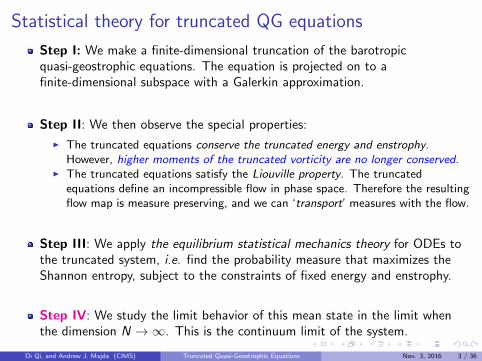
The Gibbs measure as a product of Gaussian measure




" > 0# if V = 0%

This implies either

! > 0# & > 0# (8.20)

or

V ≡ 0# ! > 0% & > −1# (8.21)

or

! < 0# & < −$# " > 0% (8.22)



V = −'

&# (

k= h

k

&+ !k!2# (8.23)

and

(′$)x# t* =

∑

1≤!k!2≤$

(keix·k% (8.24)





!!#& = c exp)−)!"$ +!&E$**

= c exp)−!)"$ +&E$**

= c!#& exp)−!#&)+q# +V**

= c!#& exp(−!

(&

2)V −V *2

+ 12

∑

1≤!k!2≤$

!k!2)!k!2 +&*)(k− (

k*2

⎞

⎠

⎞

⎠ # (8.25)

Equivalent the invariant Gibbs measure for the dynamics is a product of Gaussianmeasures with a non-zero mean�

��

Gα,µ(~X)

=N∏j=1

Gjα,µ (Xj) .


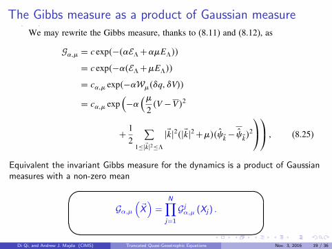
Coherent large-scale mean flow(V , ψ′Λ

)is exactly the ensemble average, or mean state, of (V , ψ′Λ) with respect

to the Gibbs measure


or equivalently

!!"#$X% =N∏

j=1!j

!"#$Xj%& (8.26)

Thus, the invariant Gibbs measure for the dynamics is a product of Gaussianmeasures with a non-zero mean. Moreover, $V "'′

(% is exactly the ensembleaverage, or mean state, of $V"'′

(% with respect to the Gibbs measure

#X$ =∫

"NX!!"#$X%dX =

(V " '

k1" & & & " '

kM

)& (8.27)

This implies, assuming ergodicity for the Gibbs measure as described in Chapter 7,the following remarkable prediction

limT→&

1T

∫ T0+T

T0

'′($x" t%dt = '

′("

limT→&

1T

∫ T0+T

T0

V$t%dt = V = −)

#&

(8.28)

Hence the statistical theory predicts that the time average of the solutions to thetruncated equations converge to the non-linearly stable exact steady state solutionsto the truncated equations. In other words, a specific coherent large-scale meanflow will emerge from the dynamics of (8.3), (8.4) with generic initial data aftercomputing a long time average.

8.4 Numerical evidence supporting the statistical prediction

The equilibrium statistical mechanics theory provides us with a striking predictionregarding the long time behavior of solutions to the spectrally truncated systems.Namely, the long time average of the solution should converge to the mostprobable mean state for generic initial data. We naturally ask if such a prediction isvalid. Instead of trying to prove the ergodicity of the Gibbs measure, an impossibletheoretical task at the present stage of our knowledge, we utilize careful numericalexperiments as we did earlier in Chapter 7. Here we report some numericalevidence supporting the convergence of the time averages of numerical solutionsto the most probable mean state predicted by the equilibrium statistical mechanicstheory in Section 8.3 for the spectrally truncated barotropic quasi-geostrophicequations on a periodic box with topography but no large-scale mean flow. Inother words, we provide numerical evidence for the validity of equation (8.28).

The statistical theory predicts that the time average of the solutions convergeto the non-linearly stable exact steady state solutions to the truncatedequations.

A specific coherent large-scale mean flow will emerge from the dynamics of(8.3), (8.4) with generic initial data after computing a long time average.


Outline






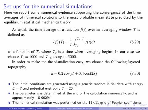
Set-ups for the numerical simulationsHere we report some numerical evidence supporting the convergence of the timeaverages of numerical solutions to the most probable mean state predicted by theequilibrium statistical mechanics theory.8.4 Numerical evidence supporting the statistical prediction 265

As usual, the time average of a function f!t" over an averaging window T isdefined as

!f"!T" = 1T

∫ T0+T

T0

f!t"dt (8.29)

as a function of T , where T0 is a time when averaging begins. In our case wechoose T0 = 1000 and T goes up to 5000.

In order to make the the visualization easy, we choose the following layeredtopography

h = 0#2 cos!x"+0#4 cos!2x" (8.30)

so that the most probable mean state predicted by the statistical theory is alsolayered, i.e. function of x only. The initial conditions are generated using ageneric random initial data with energy E = 7 and potential enstrophy ! = 20.The parameter $ is determined at the end of the calculation numerically, and isapproximately −0#9029. The numerical simulation was performed on the 11×11grid of Fourier coefficients; however, the results presented here are the streamfunctions and flows (velocity fields) on the 32 × 32 grid in physical space afterinterpolation of these results.

The convergence is measured in terms of the relative L2 error, which is definedas

L2%f& g' = %f −g%0

%f%0(8.31)

for two functions f and g.According to the above definition, L2%()& !()"!T"' denotes the relative

L2-error for the stream function, and L2%*⊥()& !*⊥()"!T"' denotes the relative

L2-error for the velocity (flow).

T L2%()& !()"!T"' L2%*⊥()& !*⊥()"!T"'

10 1#404 1#41520 1#318 1#34250 1#109 1#11670 0#8953 0#9008

100 0#4333 0#4473200 0#2451 0#2604500 0#2416 0#24961000 8#648 ·10−2 0#10175000 6#902 ·10−2 9#184 ·10−2

(8.32)

Table (8.32) lists the relative errors against the averaging window size T . As wecan see, the relative L2-errors for both stream function and velocity decrease as the

The initial conditions are generated using a generic random initial data with energyE = 7 and potential enstrophy E = 20;

The parameter µ is determined at the end of the calculation numerically, and isapproximately −0 9029;

The numerical simulation was performed on the 11×11 grid of Fourier coefficients.


Error in time-average

8.4 Numerical evidence supporting the statistical prediction 265


!f"!T" = 1T

∫ T0+T

T0

f!t"dt (8.29)



h = 0#2 cos!x"+0#4 cos!2x" (8.30)



L2%f& g' = %f −g%0

%f%0(8.31)




T L2%()& !()"!T"' L2%*⊥()& !*⊥()"!T"'

10 1#404 1#41520 1#318 1#34250 1#109 1#11670 0#8953 0#9008

100 0#4333 0#4473200 0#2451 0#2604500 0#2416 0#24961000 8#648 ·10−2 0#10175000 6#902 ·10−2 9#184 ·10−2

(8.32)

Table (8.32) lists the relative errors against the averaging window size T . As wecan see, the relative L2-errors for both stream function and velocity decrease as the

8.4 Numerical evidence supporting the statistical prediction 265


!f"!T" = 1T

∫ T0+T

T0

f!t"dt (8.29)



h = 0#2 cos!x"+0#4 cos!2x" (8.30)



L2%f& g' = %f −g%0

%f%0(8.31)




T L2%()& !()"!T"' L2%*⊥()& !*⊥()"!T"'

10 1#404 1#41520 1#318 1#34250 1#109 1#11670 0#8953 0#9008

100 0#4333 0#4473200 0#2451 0#2604500 0#2416 0#24961000 8#648 ·10−2 0#10175000 6#902 ·10−2 9#184 ·10−2

(8.32)

Table (8.32) lists the relative errors against the averaging window size T . As wecan see, the relative L2-errors for both stream function and velocity decrease as theDi Qi, and Andrew J. Majda (CIMS) Truncated Quasi-Geostrophic Equations Nov. 3, 2016 23 / 36

Time average of stream function and velocity


–3

–2

–1

0

1

2

3

4

–3 –2 –1 0 1 2–3

–2

–1

0

1

2

X

Y

–3 –2 –1 0

(a) (b)

(c) (d)

(e) (f)

1 2 3–3

– 2

–1

0

1

2

3

X

Y

–3

–2

–1

0

1

2

–3 –2 –1 0 1 2X

–1.5

–1

– 0.5

0

0.5

1

1.5

2

2.5

Y

–3 –2 –1 0 1 2 3X

–3

–2

–1

0

1

2

3Y

–3

–2

–1

0

1

2

–3 –2 –1 0 1 2X

–2

–1.5

–1

– 0.5

0

0.5

1

1.5

2

Y

–3 –2 –1 0 1 2 3X

–3

–2

–1

0

1

2

3

Y

Figure 8.1 (a) time average of stream function with T = 50, (b) time averageof velocity with T = 50, (c) time average of stream function with T = 100,(d) time average of velocity with T = 100, (e) time average of stream functionwith T = 500, (f) time average of velocity with T = 500.

averaging time increases. For a time average window of 5000, the relative erroris less than 10%. Figure 8.1 depicts the time average of the numerical solutionsover windows of size 50, 100, and 500. Figure 8.2 shows the time average ofthe numerical solutions over a window of 5000 versus the most probable mean

Figure: time average with T = 50




–3

–2

–1

0

1

2

3

4

–3 –2 –1 0 1 2–3

–2

–1

0

1

2

X

Y

–3 –2 –1 0

(a) (b)

(c) (d)

(e) (f)

1 2 3–3

– 2

–1

0

1

2

3

X

Y

–3

–2

–1

0

1

2

–3 –2 –1 0 1 2X

–1.5

–1

– 0.5

0

0.5

1

1.5

2

2.5

Y

–3 –2 –1 0 1 2 3X

–3

–2

–1

0

1

2

3

Y

–3

–2

–1

0

1

2

–3 –2 –1 0 1 2X

–2

–1.5

–1

– 0.5

0

0.5

1

1.5

2

Y

–3 –2 –1 0 1 2 3X

–3

–2

–1

0

1

2

3Y

Figure 8.1 (a) time average of stream function with T = 50, (b) time averageof velocity with T = 50, (c) time average of stream function with T = 100,(d) time average of velocity with T = 100, (e) time average of stream functionwith T = 500, (f) time average of velocity with T = 500.






–3

–2

–1

0

1

2

3

4

–3 –2 –1 0 1 2–3

–2

–1

0

1

2

X

Y

–3 –2 –1 0

(a) (b)

(c) (d)

(e) (f)

1 2 3–3

– 2

–1

0

1

2

3

X

Y

–3

–2

–1

0

1

2

–3 –2 –1 0 1 2X

–1.5

–1

– 0.5

0

0.5

1

1.5

2

2.5

Y–3 –2 –1 0 1 2 3

X

–3

–2

–1

0

1

2

3

Y

–3

–2

–1

0

1

2

–3 –2 –1 0 1 2X

–2

–1.5

–1

– 0.5

0

0.5

1

1.5

2

Y

–3 –2 –1 0 1 2 3X

–3

–2

–1

0

1

2

3

YFigure 8.1 (a) time average of stream function with T = 50, (b) time averageof velocity with T = 50, (c) time average of stream function with T = 100,(d) time average of velocity with T = 100, (e) time average of stream functionwith T = 500, (f) time average of velocity with T = 500.




Time-averaged solution with T = 5000 (left) and the mostprobable mean state (right)8.5 The pseudo-energy and equilibrium statistical mechanics 267

–1.5

–1

–0.5

0

0.5

1

1.5

2

–3 –2 –1 0 1

(a) (b)

(c) (d)

2–3

–2

–1

0

1

2

X

Y

–2

–1

–1.5

–0.5

0

0.5

1

1.5

2

–3 –2 –1 0 1 2–3

–2

–1

0

1

2

X

Y

–3 –2 –1 0 1 2 3–3

–2

–1

0

1

2

3

X

Y

–3 –2 –1 0 1 2 3–3

–2

–1

0

1

2

3

X

Y

Figure 8.2 (a) time average of stream function with T = 5000, (b) stream func-tion of the most probable mean state, (c) time average of velocity field withT = 5000, (d) velocity field of the most probable mean state.

state predicted by the equilibrium statistical theory. It is visually clear that therunning time average is close to the predicted most probable mean state for awindow size of 5000, but far from close for a window of size 50 or 100, withintermediate behavior for a window of size 500. This indicates that averagingover a sufficiently large window of time is essential for observing the predictedresults in (8.28). The specific examples for layered topography in Chapter 5 showthat such results are indeed generic in a statistical sense, i.e. not every individualsolution satisfies (8.28).

8.5 The pseudo-energy and equilibrium statistical mechanics forfluctuations about the mean

In many problems in geophysical fluids, we can assume that the time averagedmean state, the climate, is known with reasonable accuracy and that the statis-tical fluctuations about the mean state are the quantities of interest. This point


Outline






Fluctuations about the mean state

In geophysical fluids, we can assume that the time averaged mean state, theclimate, is known with reasonable accuracy and that the statistical fluctuationsabout the mean state are the quantities of interest.


of view is an important one for stochastic modeling. See for instance, Majda,Timofeyev, and Vanden Eijnden (2001). Here we show how dynamical equationsfor fluctuations and equilibrium statistical mechanics can be applied directly forthe truncated quasi-geostrophic equations treated earlier in this chapter. For sim-plicity in exposition, we assume that there is no large-scale mean flow, and theonly geophysical effect is topography, so that the equations in (8.3)–(8.4) become

!q"

!t+P"#$⊥%" ·$q"& = 0' (8.33)

We consider the exact steady solutions from (8.9) or (8.10)

q" = (%") q" = *%" +h" (8.34)

and consider perturbations about this mean state, i.e.

%" = %" + %) q" = q" + +) *% = +' (8.35)

Substituting (8.35) into (8.33) yields the equations

!+

!t+ P"#$⊥%" ·$q"&+P"#$⊥% ·$q"&+P"#$⊥%" ·$+&

+ P"#$⊥% ·$+& = 0' (8.36)

Utilizing (8.34) we have

P"#$⊥%" ·$q"& = 0)

P"#$⊥% ·$q& = (P"#$⊥% ·$%& = −(P"#$⊥% ·$%&'

Hence (8.36) becomes the equations for perturbations

!+

!t+P"#$⊥%" ·$#+−(%&&+P"#$⊥% ·$+& = 0)

*% = +'

(8.37)

The equations for perturbations involve the familiar truncated non-linear terms ofordinary fluid flow

P"#$⊥% ·$+& (8.38)

and the linear operator reflecting the mean flow %"

P"#$⊥%" ·$#+−(%&&' (8.39)

Next, we would like to set-up a statistical theory for fluctuations directly from thedynamics in (8.37). According to Chapter 7, we need to find the conserved quan-tities for (8.37) and also verify the Liouville property for the finite-dimensionalsystem of ODEs. From Section 8.2, we know that the standard non-linear terms in

We assume there is no large-scale mean flow, and the only geophysical effect istopography.


Equations for perturbations



!q"

!t+P"#$⊥%" ·$q"& = 0' (8.33)


q" = (%") q" = *%" +h" (8.34)


%" = %" + %) q" = q" + +) *% = +' (8.35)


!+

!t+ P"#$⊥%" ·$q"&+P"#$⊥% ·$q"&+P"#$⊥%" ·$+&

+ P"#$⊥% ·$+& = 0' (8.36)


P"#$⊥%" ·$q"& = 0)

P"#$⊥% ·$q& = (P"#$⊥% ·$%& = −(P"#$⊥% ·$%&'


!+

!t+P"#$⊥%" ·$#+−(%&&+P"#$⊥% ·$+& = 0)

*% = +'

(8.37)


P"#$⊥% ·$+& (8.38)


P"#$⊥%" ·$#+−(%&&' (8.39)




!q"

!t+P"#$⊥%" ·$q"& = 0' (8.33)


q" = (%") q" = *%" +h" (8.34)


%" = %" + %) q" = q" + +) *% = +' (8.35)


!+

!t+ P"#$⊥%" ·$q"&+P"#$⊥% ·$q"&+P"#$⊥%" ·$+&

+ P"#$⊥% ·$+& = 0' (8.36)


P"#$⊥%" ·$q"& = 0)

P"#$⊥% ·$q& = (P"#$⊥% ·$%& = −(P"#$⊥% ·$%&'


!+

!t+P"#$⊥%" ·$#+−(%&&+P"#$⊥% ·$+& = 0)

*% = +'

(8.37)


P"#$⊥% ·$+& (8.38)


P"#$⊥%" ·$#+−(%&&' (8.39)



Conserved quantities for (8.37)

We would like to set-up a statistical theory for fluctuations directly from thedynamics in (8.37).

The standard non-linear terms, PΛ

(∇⊥ψ · ∇ω

), conserve both the energy

and enstrophy;

The linear operator, PΛ

(∇⊥ψΛ · ∇

(ω − µψ

)), conserves neither the energy

nor the enstrophy.

The non-linear stability analysis suggests that there exists a single conservedquantity, E , involving fluctuations about the mean state given by thepseudo-energy�

�� E =

1

2

(ω2 − µψω

)= EΛ + µEΛ.


Conservation of pseudo-energy

We focus only on the contribution arising from the linear terms, since thenon-linear terms automatically conserve both energy and enstrophy separately.

8.5 The pseudo-energy and equilibrium statistical mechanics 269

(8.38) conserve the energy and enstrophy; however, the linear operator in (8.39)conserves neither the energy nor the enstrophy. Nevertheless, the non-linear sta-bility analysis from Section 4.2 and equation (8.12) suggests that there exists asingle conserved quantity, E, for the dynamics in (8.37), involving fluctuationsabout the mean state given by the pseudo-energy

E = 12

∫− !"2 −#$"% = !& +#E&' (8.40)

which is an appropriate linear combination of energy and enstrophy. To check theconservation of the pseudo-energy directly for the dynamic equations in (8.37),we focus only on the contribution arising from the linear terms in (8.39), sincethe non-linear terms in (8.38) automatically conserve both energy and enstrophyseparately. We calculate from (8.37) and (8.39) that

dE

dt=∫− !"−#$%

("

(t

= −∫− !"−#$%)⊥$& ·)!"−#$%

= −∫−)⊥$& ·)

(12

!"−#$%2)

= 0' (8.41)

which verifies the conservation of the pseudo-energy.From Section 4.2 and Subsection 8.2.3, the quadratic form defining the pseudo-

energy in (8.40) is given by

E = 12

∑

#k#2≤&

(

1+ #

#k#2

)

#"k#2 (8.42)

and is positive definite only for # > −1 for arbitrary truncations &. In this case,we introduce the pseudo-energy variables, p

k, defined by

pk=(

1+ #

#k#2

)1/2

"k* (8.43)

Next we sketch how to set up equilibrium statistical mechanics directly for thefluctuation described by the dynamic equations (8.37).

With (8.43) we use the natural coordinates

X =(

Re pk1

' Im pk1

' * * * ' Re pkM

' Im pkM

)(8.44)

over a suitably defining set S as in (8.13)–(8.14). It is a straightforward exercisefor the reader to check that the Liouville property is satisfied directly for the


Checking Liouville property



E = 12

∫− !"2 −#$"% = !& +#E&' (8.40)


dE

dt=∫− !"−#$%

("

(t

= −∫− !"−#$%)⊥$& ·)!"−#$%

= −∫−)⊥$& ·)

(12

!"−#$%2)

= 0' (8.41)



E = 12

∑

#k#2≤&

(

1+ #

#k#2

)

#"k#2 (8.42)


k, defined by

pk=(

1+ #

#k#2

)1/2

"k* (8.43)



X =(

Re pk1

' Im pk1

' * * * ' Re pkM

' Im pkM

)(8.44)

over a suitably defining set S as in (8.13)–(8.14). It is a straightforward exercisefor the reader to check that the Liouville property is satisfied directly for the



E = 12

∫− !"2 −#$"% = !& +#E&' (8.40)


dE

dt=∫− !"−#$%

("

(t

= −∫− !"−#$%)⊥$& ·)!"−#$%

= −∫−)⊥$& ·)

(12

!"−#$%2)

= 0' (8.41)



E = 12

∑

#k#2≤&

(

1+ #

#k#2

)

#"k#2 (8.42)


k, defined by

pk=(

1+ #

#k#2

)1/2

"k* (8.43)



X =(

Re pk1

' Im pk1

' * * * ' Re pkM

' Im pkM

)(8.44)

over a suitably defining set S as in (8.13)–(8.14). It is a straightforward exercisefor the reader to check that the Liouville property is satisfied directly for theIt is straightforward to check that the Liouville property is satisfied directly for the

fluctuation dynamics with the variables in (8.43).Di Qi, and Andrew J. Majda (CIMS) Truncated Quasi-Geostrophic Equations Nov. 3, 2016 31 / 36

Equilibrium statistical Gibbs measure for the fluctuations

The equilibrium statistical theory applies directly to the fluctuations with theequilibrium statistical Gibbs measure given by

Gα = Cα exp(−αE

)= Cα exp

(−α

2

∑∣∣p~k ∣∣2) .This Gibbs measure for fluctuations has the same structure in thepseudo-energy variables as the Gibbs measure for the truncated Burgersequations;

This leads to predictions of equi-partition of pseudo-energy for fluctuationsabout the mean state as the truncated Burgers equation;The same result would have been obtained directly from the approach bymerely diagonalizing the quadratic form in (8.25)

Gα,µ = cα,µ exp

[−α

(µ

2

(V − V

)2+

1

2

∑|k|2

(|k|2 + µ

)(ψk − ψk

)2)]

.


Numerical results confirming the equi-partition ofpseudo-energy


0 5 10 15 20 25 30 35 40 45 500

0.050.1

0.150.2

0.250.3

0.350.4

0.450.5

(a) (b)

pseu

do-e

nerg

y

0 50 100 150 2000

0.010.020.030.040.050.060.070.080.090.1

pseu

do-e

nerg

y

Figure 8.3 Pseudo-energy spectrum. Solid line with circles – numerical result,dashed line – analytical prediction. (a) 11 × 11 case: ! = 4"355#$ = −0"9029,(b) 23×23 case: ! = 19"52#$ = −0"9545.

dynamics (8.37) with the variables in (8.43) with the same structure as (8.16)and (8.17). Thus the equilibrium statistical theory developed in Chapter 7 appliesdirectly to the fluctuations with the equilibrium statistical Gibbs measure givenby

!! = C!e−!E = C!e− !2∑ #p

k#2 " (8.45)

This Gibbs measure for fluctuations has the same structure in the pseudo-energyvariables as the Gibbs measure for the truncated Burgers equations in Section 7.3and leads to predictions of equi-partition of pseudo-energy for fluctuations aboutthe mean state as in Chapter 7 for the truncated Burgers equation. Clearly, the sameresult would have been obtained directly from the approach in Sections 8.2 and 8.3by merely diagonalizing the quadratic form in (8.25); however, the dynamic statis-tical theory for fluctuations developed here has independent interest and providesan alternative point of view which we emphasize here. Figure 8.3 contains numer-ical results confirming the equi-partition of pseudo-energy predicted by (8.45).The numerical simulation is carried out in exactly the same way as described inSection 8.4 with the same layered topography given by (8.30). The pseudo-energyin each mode is calculated using time average just as in Subsection 7.3.4. It isvisually clear that the equi-partition of energy holds very well.

8.6 The continuum limit

Recall that we are interested in the dynamics of the quasi-geostrophic equations(8.1). It is only in the limit of % → & that we recover the solution to (8.1) fromsolutions to the truncated equations (8.3), (8.4). Thus we are naturally interested


A list of the topics that we have studied in the previouslectures

i) Exact solutions showing interesting physics

ii) Conserved quantities

iii) Response to large-scale forcing

iv) Large- and small-scale interaction via topographic stress.

v) Non-linear stability of certain steady geophysical flows

vi) Equilibrium statistics mechanics and statistical theories for largecoherent structures

vii) Dynamic modeling for geophysical flows

viii) How information theory can be used to quantify predictability forensemble predictions in geophysical flows


Modern Applied Math Paradigm

Modern Applied Math Paradigm

Rigorous Math Theory

Qualitative orQuantitativeModels

Novel NumericalAlgorithm

Crucial Improved Understanding ofComplex System

3 / 51


Questions & Discussions


Statistical Mechanics for the Truncated Quasi-Geostrophic ...

Documents

Transcript of Statistical Mechanics for the Truncated Quasi-Geostrophic ...