Earth’s Circulation Atmospheric Circulation Ocean Circulation.
Statistical-mechanical forcing of ocean circulation
Bill Merryfield
Canadian Centre for Climate Modelling
and Analysis
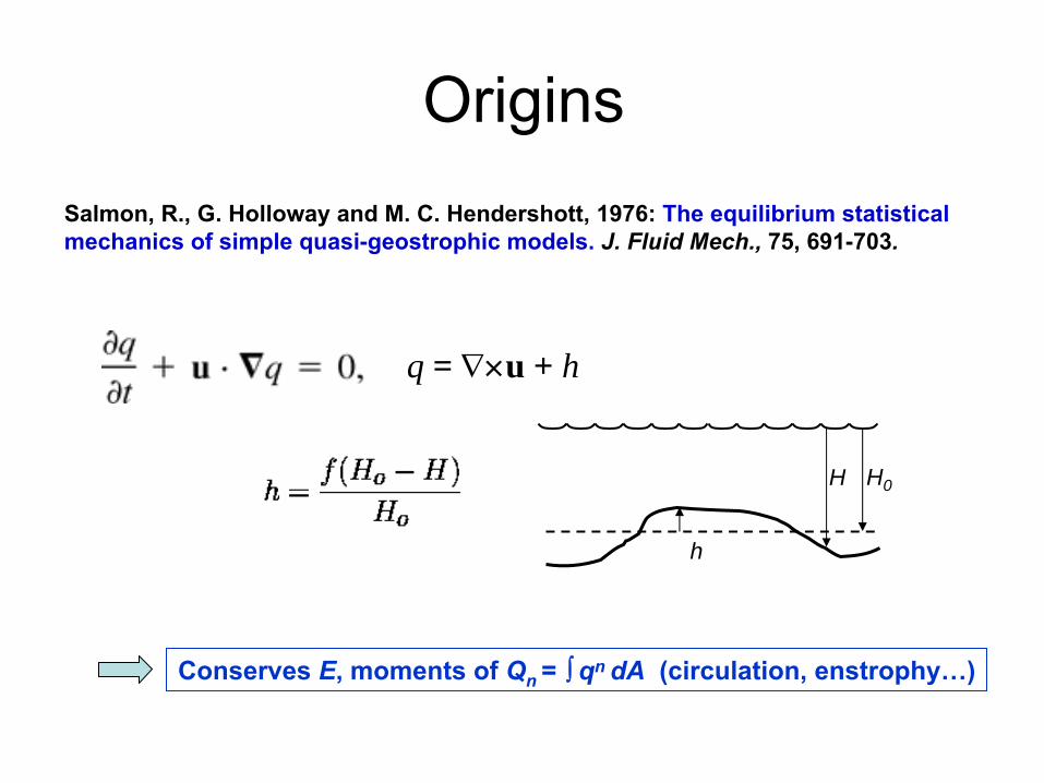
OriginsSalmon, R., G. Holloway and M. C. Hendershott, 1976: The equilibrium statistical mechanics of simple quasi-geostrophic
models.
J. Fluid Mech., 75, 691-703.
q = ∇×u + h
H0H
h
Conserves E, moments of Qn
= ∫
qn
dA
(circulation, enstrophy…)
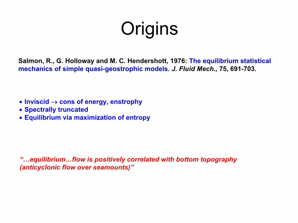
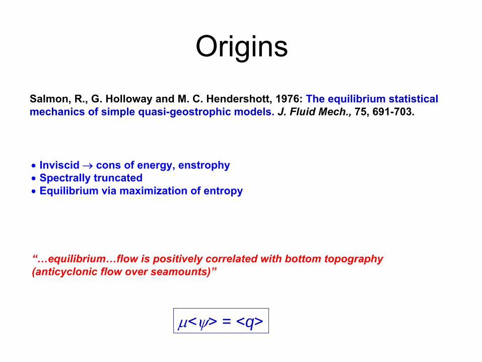
OriginsSalmon, R., G. Holloway and M. C. Hendershott, 1976: The equilibrium statistical mechanics of simple quasi-geostrophic
models.
J. Fluid Mech., 75, 691-703.
“…equilibrium…flow is positively correlated with bottom topography (anticyclonic
flow over seamounts)”
• Inviscid
→ cons of energy, enstrophy• Spectrally truncated• Equilibrium via maximization of entropy
μ<ψ> = <q>
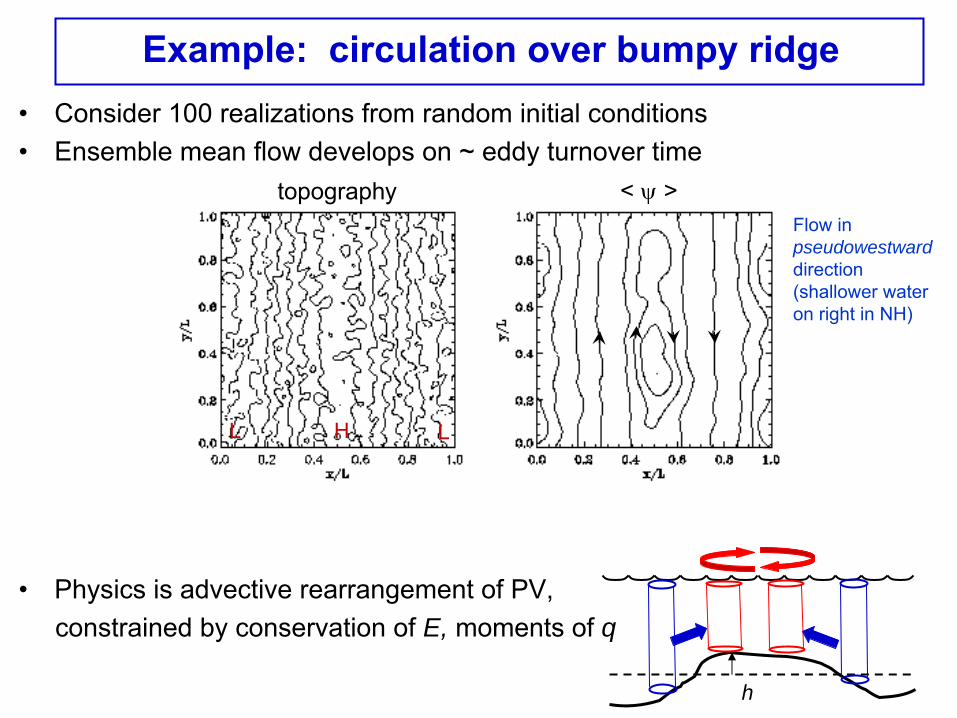
Example: circulation over bumpy ridge •
Consider 100 realizations from random initial conditions •
Ensemble mean flow develops on ~ eddy turnover timetopography < ψ
>
H LL
•
Physics is advective
rearrangement of PV, constrained by conservation of E, moments of q
h
Flow in pseudowestward direction (shallower water on right in NH)
What is Entropy?
•
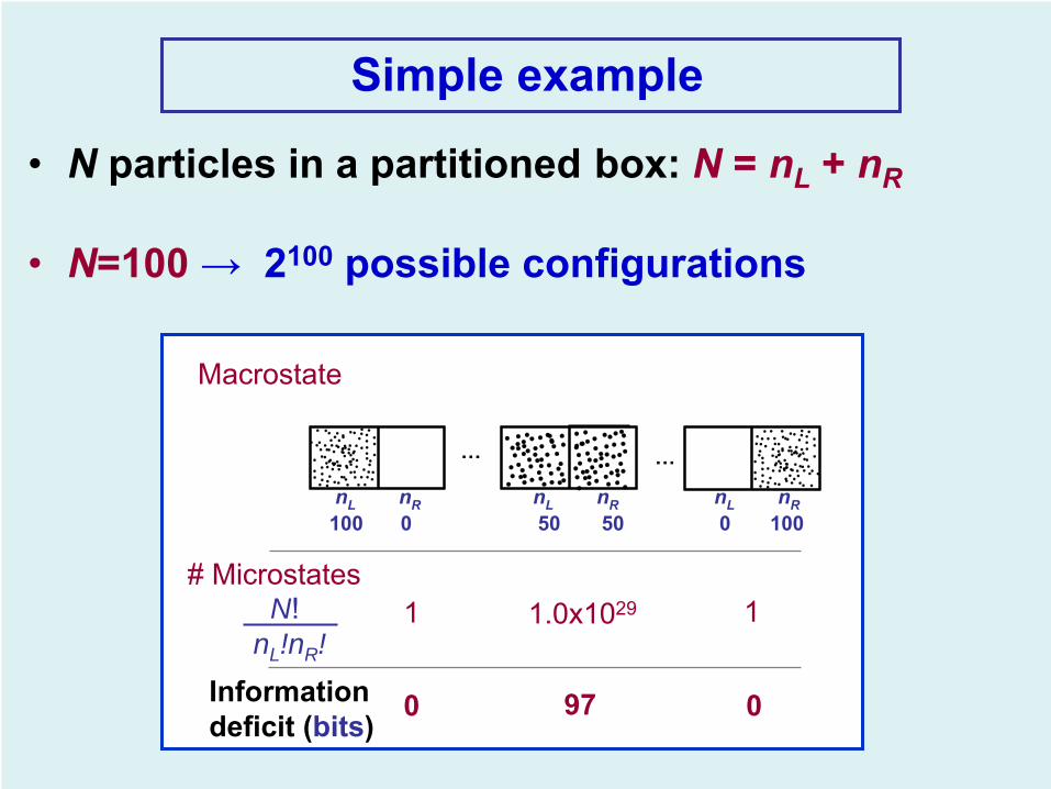
Entropy is the INFORMATION DEFICIT between detailed knowledge (microstate)
and statistical knowledge (macrostate) of a system
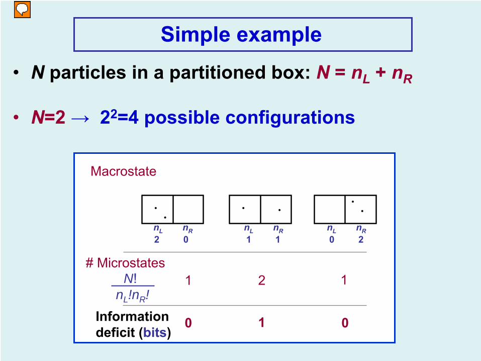
Simple example
•
N particles in a partitioned box: N = nL
+ nR
•
N=2 →
22=4 possible configurations
1 2 1
0 1 0Informationdeficit (bits)
# MicrostatesN!
nL !nR !
Macrostate
•
•
• • •
•
nL nR nL nR nL nR2 0 1 1 0 2
Simple example
1 1.0x1029 1
0 97 0Informationdeficit (bits)
# MicrostatesN!
nL !nR !
Macrostate
nL nR nL nR nL nR100 0 50 50 0 100
•
N particles in a partitioned
box: N = nL
+ nR
•
N=100 →
2100
possible configurations
… …•
••
• ••
•
•
•
•
•
••
•••
••
•
•
•
••
•••
••
•
••
••
•••
••
•
•
•
••
••
•
•
•
••
•
••
••
•
•
•
••
•
••
•••
•
•
•
•
•
••
•••
•
•
•
•
•
••
• ••
•
•
•
•
•
••
• ••
•
•
•
•
•
••
•••
•
•
•
•
•
••
•• •
••
•
•
•
••
•• •
••
•
••
••
•• •
••
•
•
•
• •
••
•
•
•
• •
•
• •
••
•
•
•
• •
•
••
• ••
•
•
•
•
•
••
• ••
•
•
•
•
•
••
•••
•
•
•
•
•
••
•••
•
•
•
•
• •••• ••
• •• •
••• ••• •
••
•••• ••
•
•••
•••• • •
• •••
•• ••• •••
• • •• ••••••
•
•
•
•••• ••
••
•
• •••• • •
• ••
• ••••
••• • •
••• • •
• • •••
•
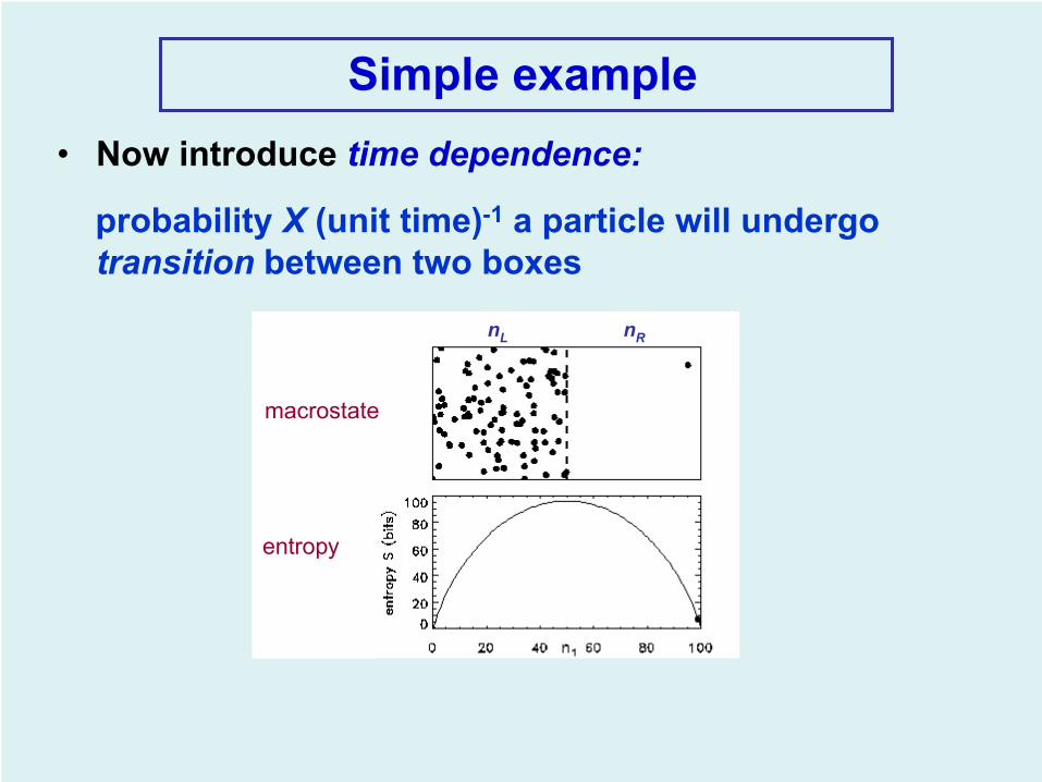
Now introduce time dependence:
probability X
(unit time)-1
a particle will undergo transition
between two boxes
nL nR
macrostate
entropy
Simple example
•
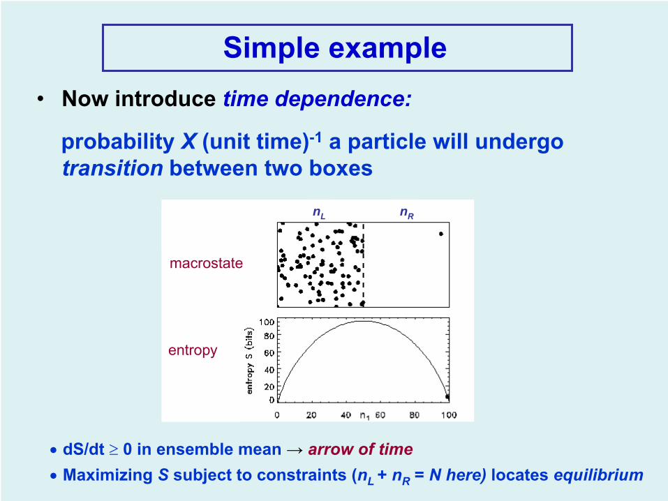
Now introduce time dependence:
probability X
(unit time)-1
a particle will undergo transition
between two boxes
nL nR
macrostate
entropy
Simple example
• dS/dt
≥
0 in ensemble mean → arrow of time• Maximizing S subject to
constraints (nL
+ nR
= N here) locates equilibrium
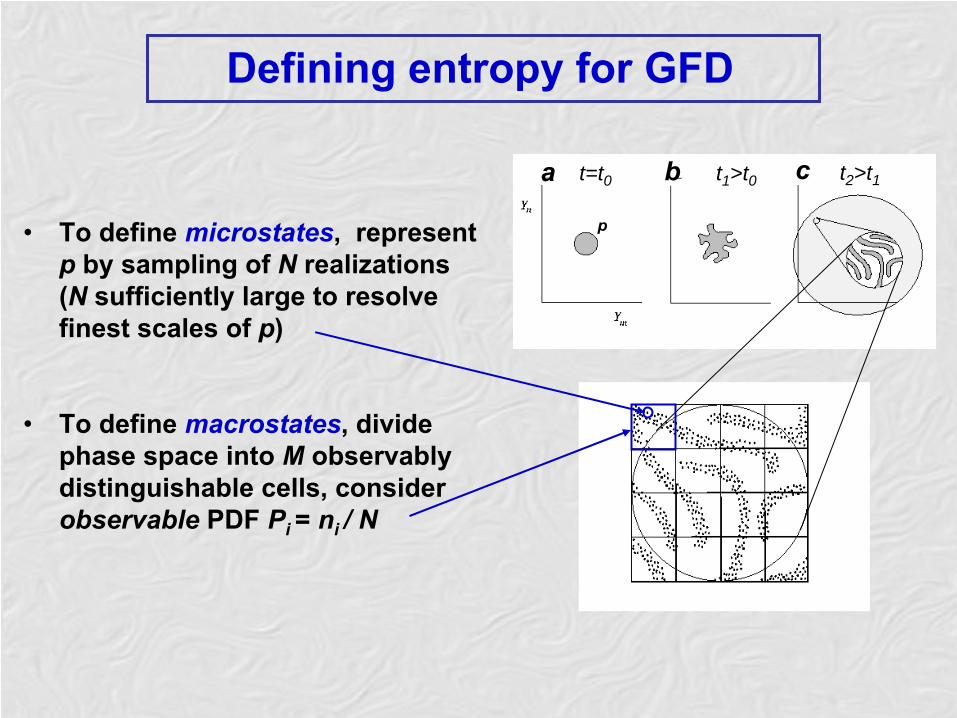
Defining entropy for GFD
•
To define microstates, represent p
by sampling of N
realizations (N sufficiently large to resolve finest scales of p)
•
To define macrostates, divide phase space into M observably distinguishable cells, consider observable PDF Pi = ni
/ N
a b c
p
t=t0 t1 >t0 t2 >t1
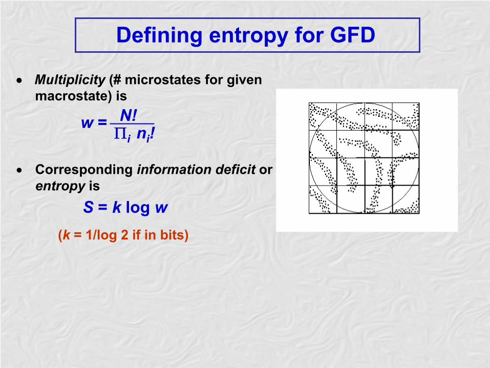
Defining entropy for GFD
•
Multiplicity (# microstates for given macrostate) is
•
Corresponding
information deficit or entropy
is
(k = 1/log 2 if in bits)
w = N!Πi
ni
!
S = k log w
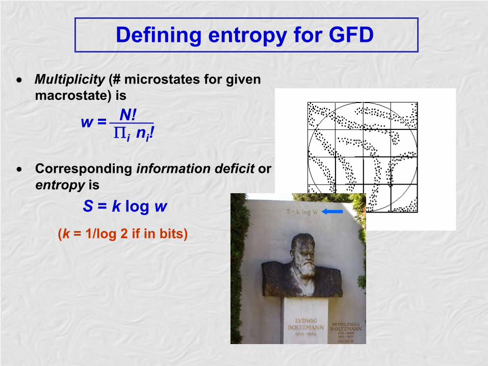
Defining entropy for GFD
•
Multiplicity (# microstates for given macrostate) is
•
Corresponding
information deficit or entropy
is
(k = 1/log 2 if in bits)
w = N!Πi
ni
!
S = k log w
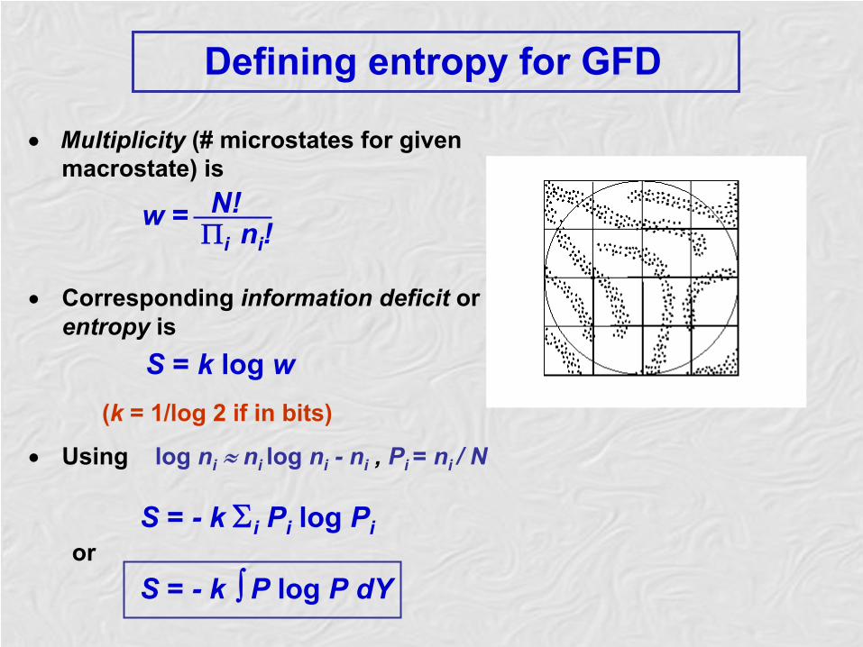
Defining entropy for GFD
•
Multiplicity (# microstates for given macrostate) is
•
Corresponding
information deficit or entropy
is
(k = 1/log 2 if in bits)
•
Using log ni
≈ ni
log ni
- ni
, Pi = ni
/ N
w = N!Πi
ni
!
S = k log w
S = -
k Σi
Pi
log Pi
S = -
k ∫
P log P dYor
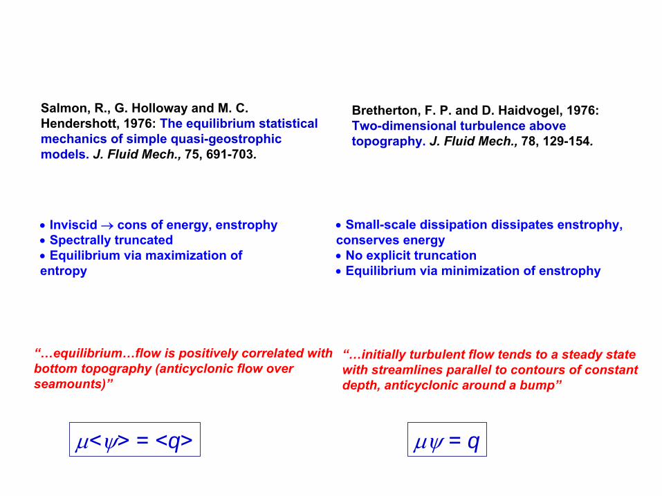
Bretherton, F. P. and D. Haidvogel, 1976: Two-dimensional turbulence above topography.
J. Fluid Mech., 78, 129-154.
“…equilibrium…flow is positively correlated with bottom topography (anticyclonic
flow over seamounts)”
“…initially turbulent flow tends to a steady state with streamlines parallel to contours of constant depth, anticyclonic
around a bump”
• Inviscid
→ cons of energy, enstrophy• Spectrally truncated•
Equilibrium via maximization of entropy
•
Small-scale dissipation dissipates enstrophy, conserves energy • No explicit truncation• Equilibrium via minimization of enstrophy
μ<ψ> = <q> μψ = q
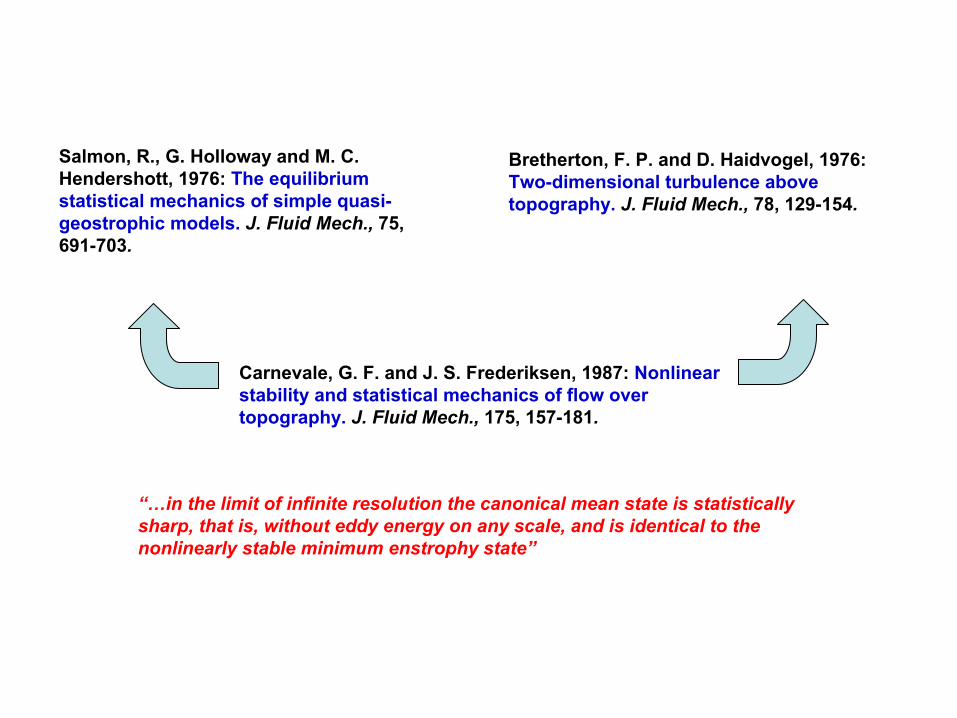
Salmon, R., G. Holloway and M. C. Hendershott, 1976: The equilibrium statistical mechanics of simple quasi-geostrophic
models.
J. Fluid Mech., 75, 691-703.
Salmon, R., G. Holloway and M. C. Hendershott, 1976: The equilibrium statistical mechanics of simple quasi-
geostrophic
models.
J. Fluid Mech., 75, 691-703.
Bretherton, F. P. and D. Haidvogel, 1976: Two-dimensional turbulence above topography.
J. Fluid Mech., 78, 129-154.
“…in the limit of infinite resolution the canonical mean state is statistically sharp, that is, without eddy energy on any scale, and is identical to the nonlinearly stable minimum enstrophy
state”
Carnevale, G. F. and J. S. Frederiksen, 1987: Nonlinear stability and statistical mechanics of flow over topography.
J. Fluid Mech., 175, 157-181.
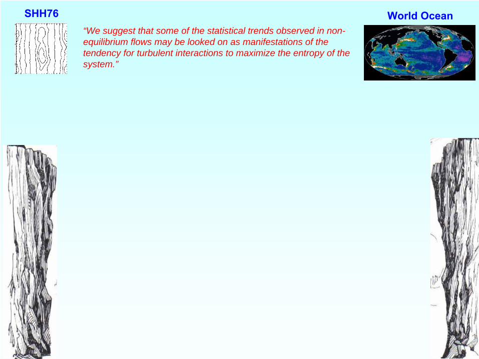
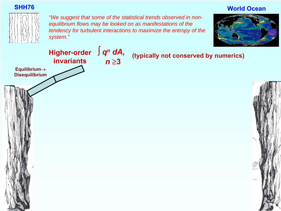
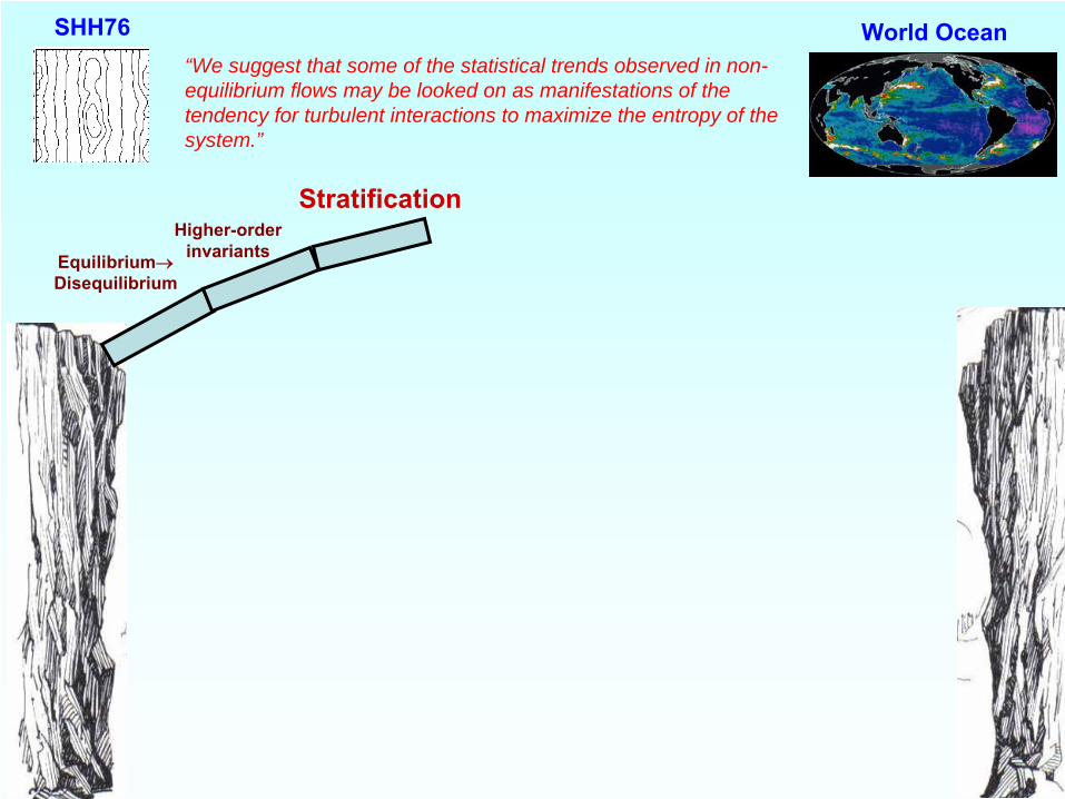
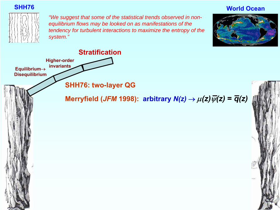
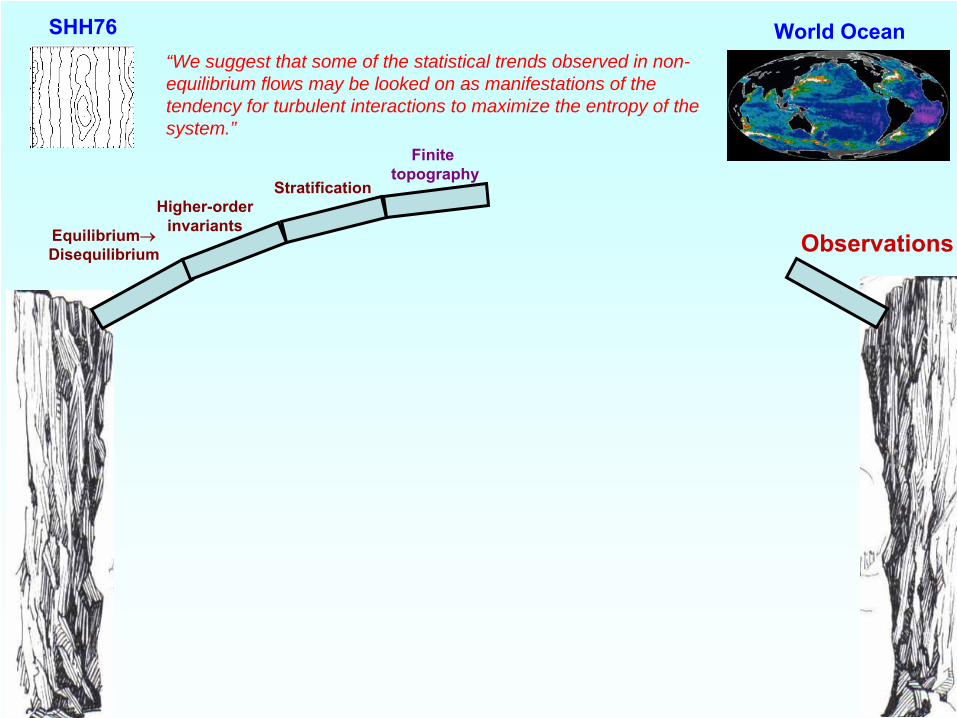
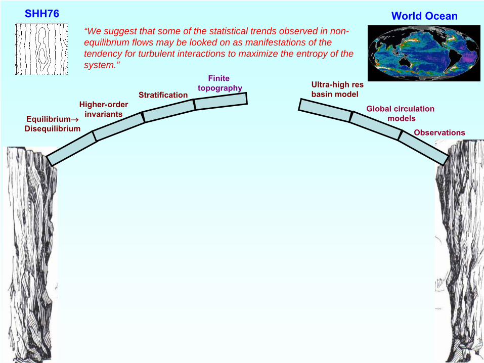
SHH76 World Ocean“We suggest that some of the statistical trends observed in non- equilibrium flows may be looked on as manifestations of the tendency for turbulent interactions to maximize the entropy of the system.”
SHH76 World Ocean
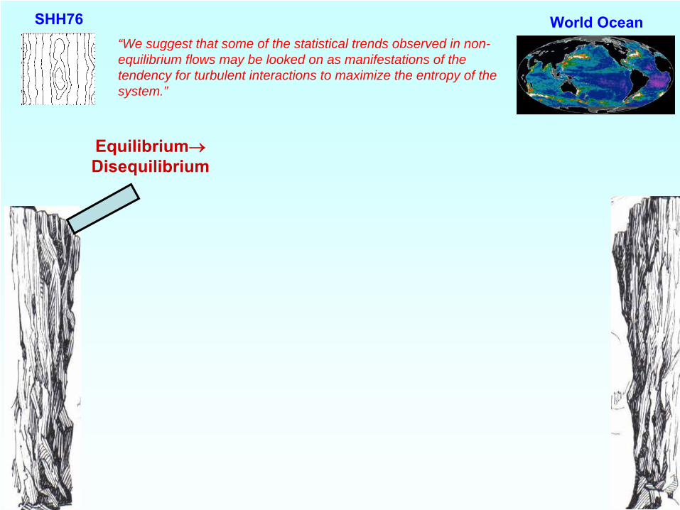
Equilibrium→Disequilibrium
“We suggest that some of the statistical trends observed in non- equilibrium flows may be looked on as manifestations of the tendency for turbulent interactions to maximize the entropy of the system.”
SHH76 World Ocean
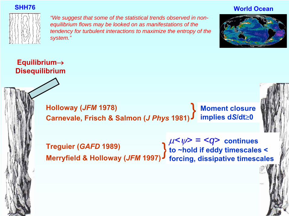
Equilibrium→Disequilibrium
“We suggest that some of the statistical trends observed in non- equilibrium flows may be looked on as manifestations of the tendency for turbulent interactions to maximize the entropy of the system.”
Treguier
(GAFD 1989)Merryfield & Holloway (JFM 1997)
Holloway (JFM 1978)Carnevale, Frisch & Salmon (J Phys
1981)} Moment closure implies dS/dt≥0
}μ<ψ> = <q>
continues
to ~hold if eddy timescales < forcing, dissipative timescales
•
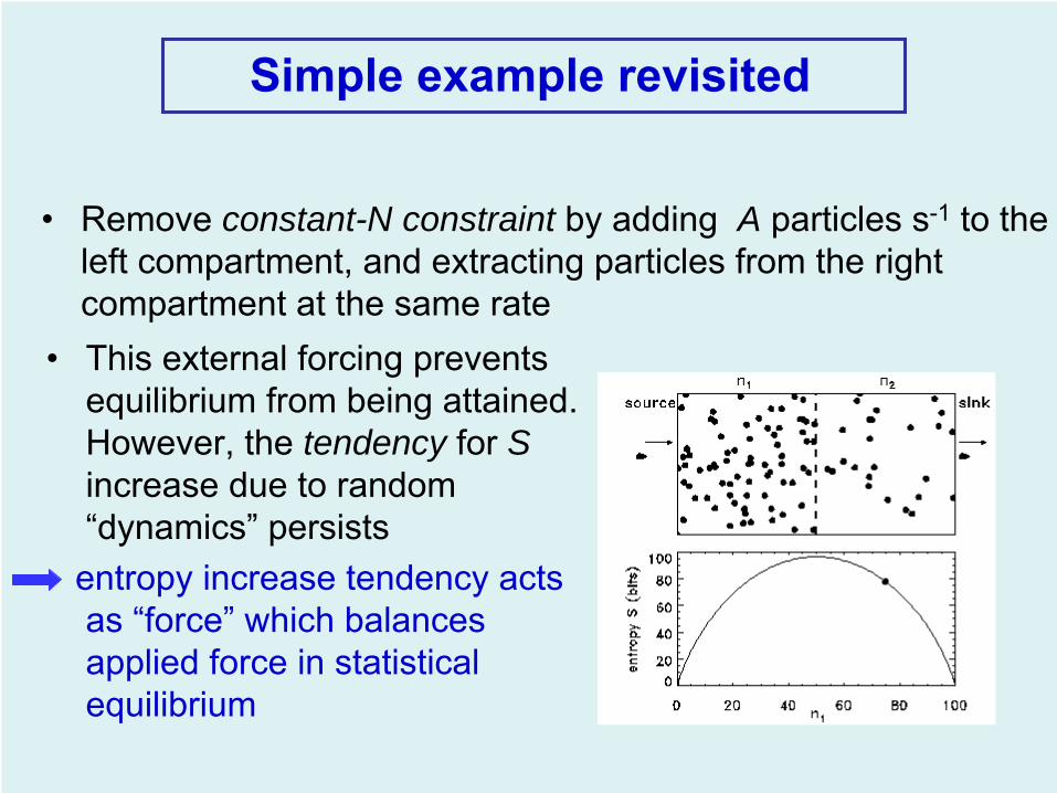
Remove constant-N constraint by adding A particles s-1
to the left compartment, and extracting particles from the right compartment at the same rate
•
This external forcing prevents equilibrium from being attained. However, the tendency for S increase due to random “dynamics”
persists
entropy increase tendency acts as “force”
which balances
applied force in statistical equilibrium
Simple example revisited
SHH76 World Ocean
Equilibrium→Disequilibrium
“We suggest that some of the statistical trends observed in non- equilibrium flows may be looked on as manifestations of the tendency for turbulent interactions to maximize the entropy of the system.”
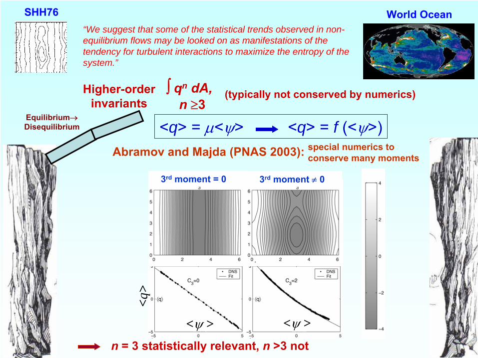
Higher-orderinvariants
∫
qn
dA, n ≥3
(typically not conserved by numerics)

SHH76 World Ocean
Equilibrium→Disequilibrium
“We suggest that some of the statistical trends observed in non- equilibrium flows may be looked on as manifestations of the tendency for turbulent interactions to maximize the entropy of the system.”
Higher-orderinvariants
∫
qn
dA, n ≥3
(typically not conserved by numerics)
<q> = μ<ψ> <q> = f (<ψ>)
SHH76 World Ocean
Equilibrium→Disequilibrium
“We suggest that some of the statistical trends observed in non- equilibrium flows may be looked on as manifestations of the tendency for turbulent interactions to maximize the entropy of the system.”
Higher-orderinvariants
Abramov
and Majda
(PNAS 2003):
∫
qn
dA, n ≥3
(typically not conserved by numerics)
<q> = μ<ψ> <q> = f (<ψ>)
n = 3 statistically relevant, n >3 not
special numerics
to conserve many moments
3rd
moment = 0 3rd
moment ≠
0
<q>
<ψ ><ψ >
SHH76 World Ocean
Equilibrium→Disequilibrium
“We suggest that some of the statistical trends observed in non- equilibrium flows may be looked on as manifestations of the tendency for turbulent interactions to maximize the entropy of the system.”
Higher-orderinvariants
Stratification
SHH76 World Ocean
Equilibrium→Disequilibrium
“We suggest that some of the statistical trends observed in non- equilibrium flows may be looked on as manifestations of the tendency for turbulent interactions to maximize the entropy of the system.”
Higher-orderinvariants
Stratification
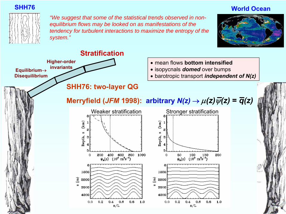
Merryfield (JFM 1998): arbitrary N(z) → μ(z)ψ(z) = q(z)
SHH76: two-layer QG
SHH76 World Ocean
Equilibrium→Disequilibrium
“We suggest that some of the statistical trends observed in non- equilibrium flows may be looked on as manifestations of the tendency for turbulent interactions to maximize the entropy of the system.”
Higher-orderinvariants
Stratification
Merryfield (JFM 1998): arbitrary N(z) → μ(z)ψ(z) = q(z)
SHH76: two-layer QG
Weaker stratification Stronger stratification
• mean flows bottom intensified• isopycnals
domed over bumps• barotropic
transport independent of N(z)
Equilibrium→Disequilibrium
Higher-orderinvariants
Stratification
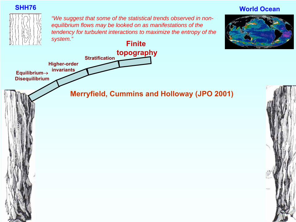
Finite topography
Merryfield, Cummins and Holloway (JPO 2001)
SHH76 World Ocean“We suggest that some of the statistical trends observed in non- equilibrium flows may be looked on as manifestations of the tendency for turbulent interactions to maximize the entropy of the system.”
Equilibrium→Disequilibrium
Higher-orderinvariants
Stratification
Finite topography
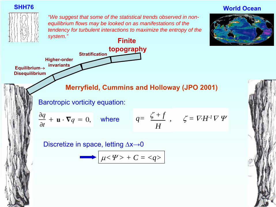
Merryfield, Cummins and Holloway (JPO 2001)
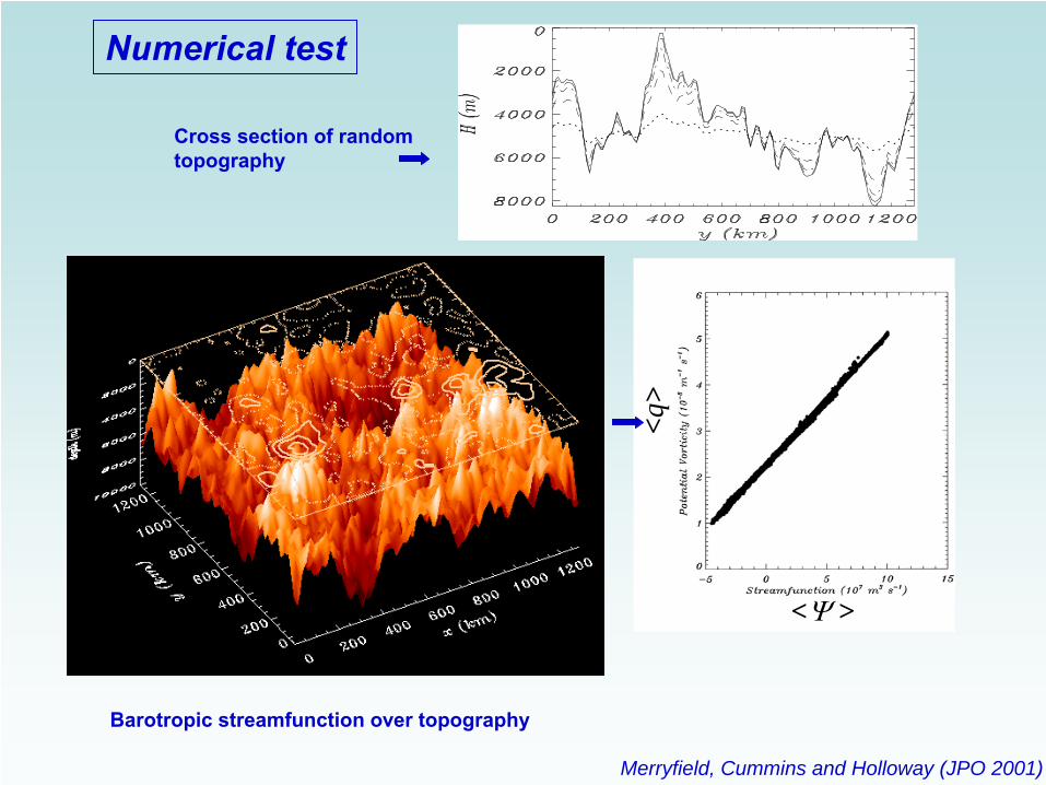
Barotropic
vorticity
equation:
where q= ζ + fH
, ζ =∇⋅H-1∇ Ψ
Discretize
in space, letting Δx→0
μ<Ψ > + C = <q>
SHH76 World Ocean“We suggest that some of the statistical trends observed in non- equilibrium flows may be looked on as manifestations of the tendency for turbulent interactions to maximize the entropy of the system.”
<q>
<Ψ >
Numerical test
Merryfield, Cummins and Holloway (JPO 2001)
Cross section of random topography
Barotropic
streamfunction
over topography

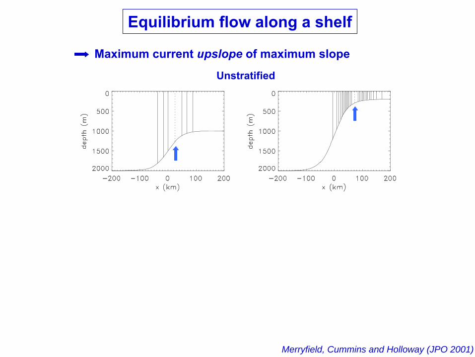
Equilibrium flow along a shelf
Merryfield, Cummins and Holloway (JPO 2001)
Unstratified
Equilibrium flow along a shelf
Merryfield, Cummins and Holloway (JPO 2001)
Unstratified
Maximum current upslope
of maximum slope
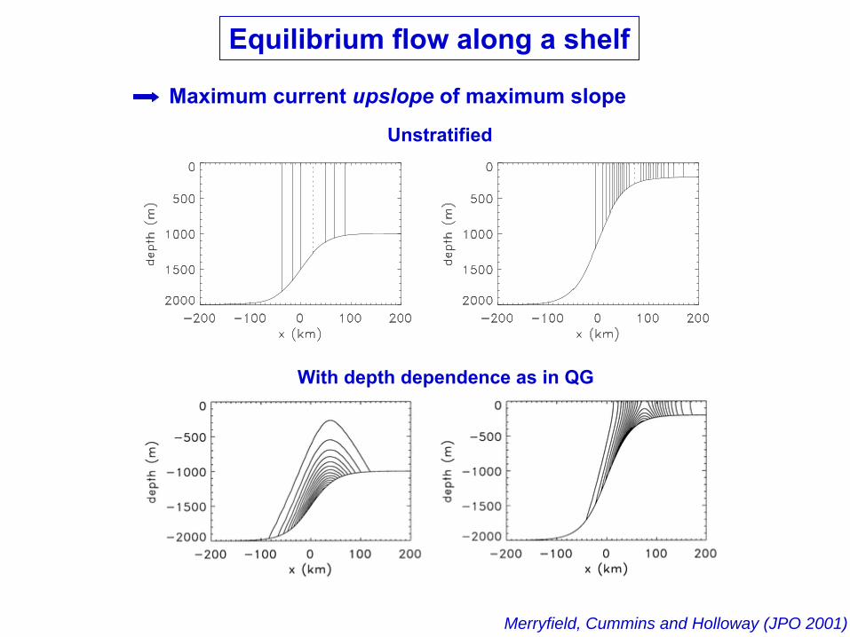
Equilibrium flow along a shelf
Merryfield, Cummins and Holloway (JPO 2001)
Unstratified
With depth dependence as in QG
Maximum current upslope
of maximum slope
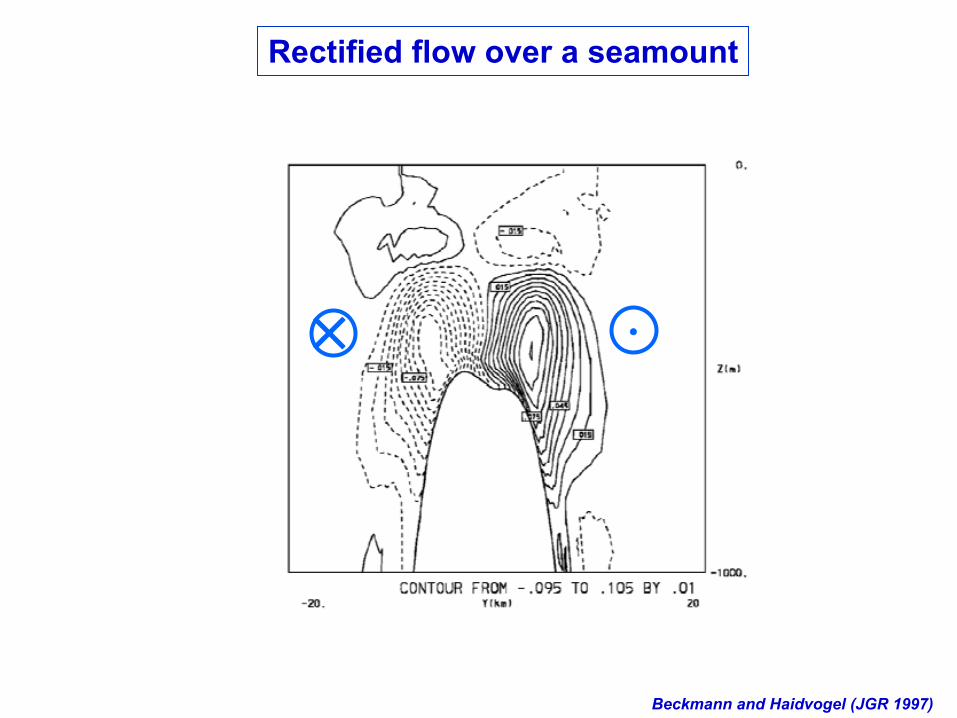
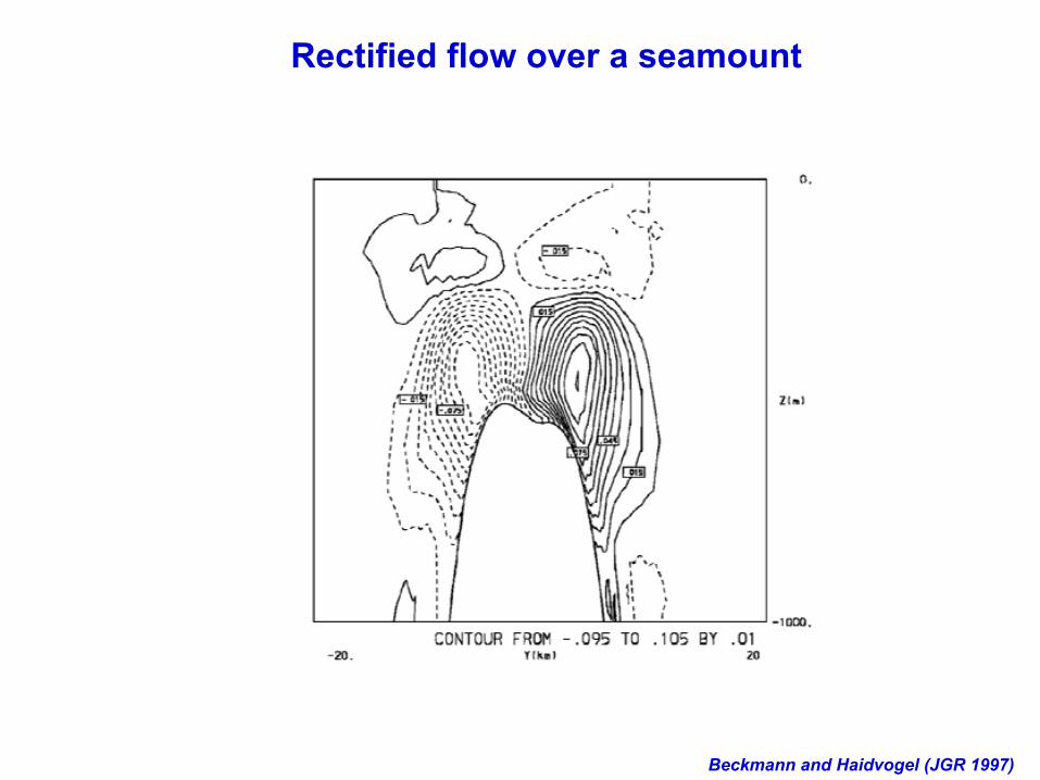
Rectified flow over a seamount
Beckmann and Haidvogel
(JGR 1997)
•×
SHH76 World Ocean“We suggest that some of the statistical trends observed in non- equilibrium flows may be looked on as manifestations of the tendency for turbulent interactions to maximize the entropy of the system.”
Equilibrium→Disequilibrium
Higher-orderinvariants
Stratification
Finite topography
Observations
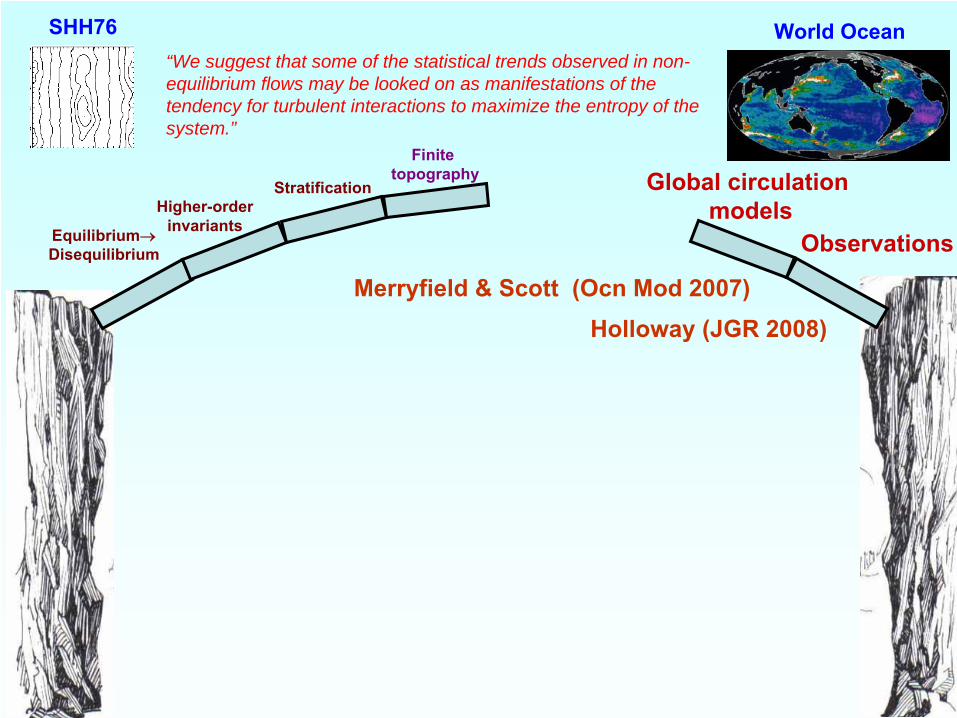
Global circulation models
Merryfield & Scott (Ocn
Mod 2007)Holloway (JGR 2008)
SHH76 World Ocean“We suggest that some of the statistical trends observed in non- equilibrium flows may be looked on as manifestations of the tendency for turbulent interactions to maximize the entropy of the system.”
Equilibrium→Disequilibrium
Higher-orderinvariants
Stratification
Finite topography
Observations
Global circulation models
Merryfield & Scott (Ocn
Mod 2007)Holloway (JGR 2008)
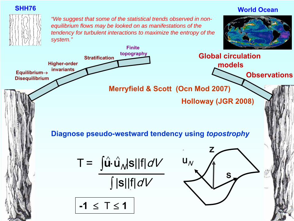
∧z
∧s
∧
uN∫u⋅uN
|s||f|dV|s||f|dV∫
∧
∧T = ∧
-1 ≤
T
≤
1
Diagnose pseudo-westward tendency using topostrophy
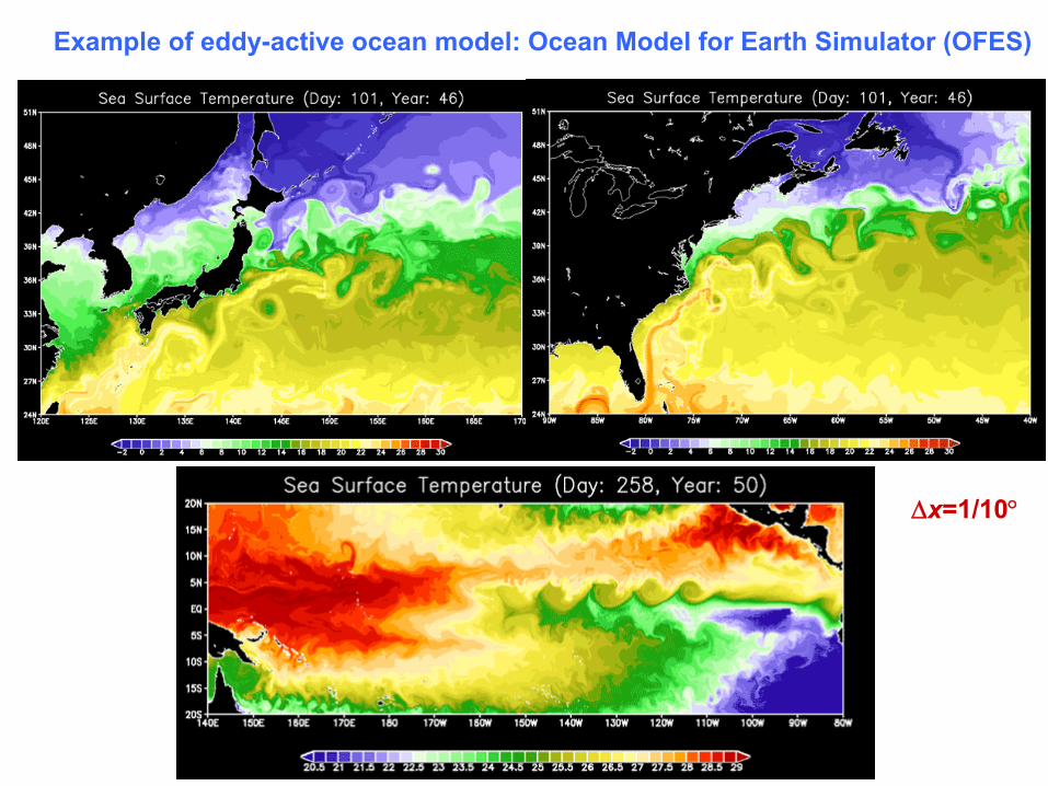
Example of eddy-active ocean model: Ocean Model for Earth Simulator (OFES)
Δx=1/10°
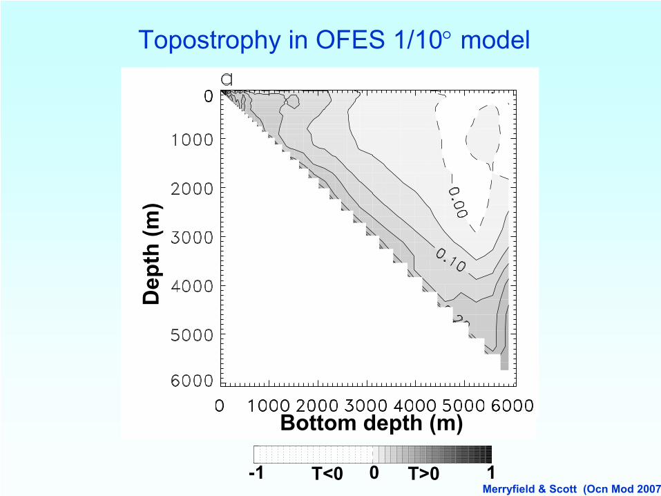
Topostrophy
in OFES 1/10°
model
-1 0 1T<0 T>0
Dep
th (m
)
Bottom depth (m)
Merryfield & Scott (Ocn
Mod 2007)
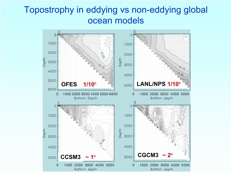
-1 0 1T<0 T>0
Bottom depth (m)
Topostrophy
in eddying vs
non-eddying global ocean models
OFES LANL/NPS1/10° 1/10°
CCSM3 ~ 1° CGCM3 ~ 2°
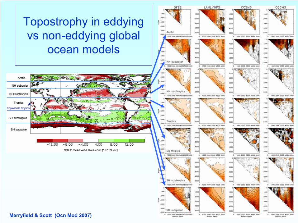
Topostrophy
in eddying vs
non-eddying global ocean models
Merryfield & Scott (Ocn
Mod 2007)
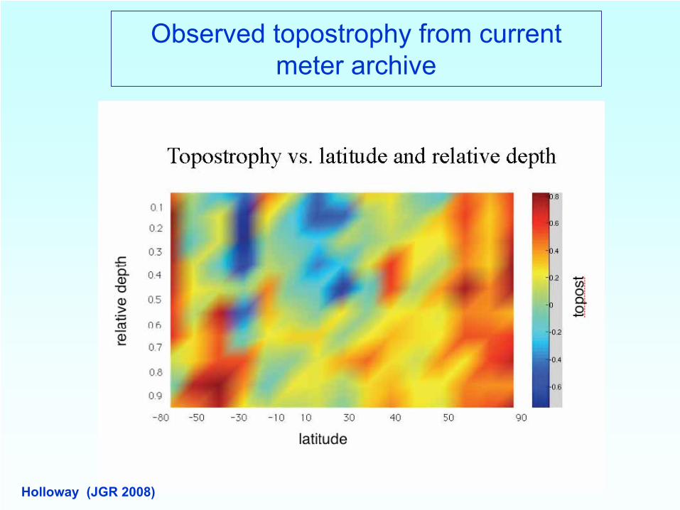
Observed topostrophy
from current meter archive
Holloway (JGR 2008)
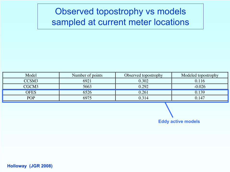
Observed topostrophy
vs
models sampled at current meter locations
Holloway (JGR 2008)
Model Number of points Observed topostrophy Modeled topostrophyCCSM3 6921 0.302 0.116CGCM3 5663 0.292 -0.026OFES 6526 0.261 0.139POP 6975 0.314 0.147
Eddy active models
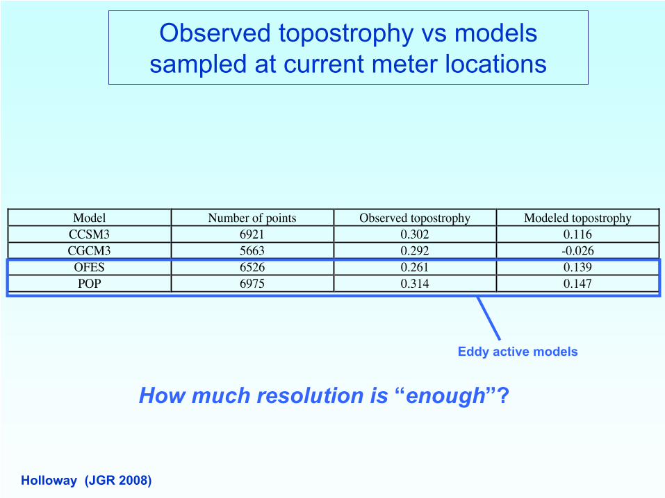
Observed topostrophy
vs
models sampled at current meter locations
Holloway (JGR 2008)
Model Number of points Observed topostrophy Modeled topostrophyCCSM3 6921 0.302 0.116CGCM3 5663 0.292 -0.026OFES 6526 0.261 0.139POP 6975 0.314 0.147
Eddy active models
How much resolution is
“enough”?
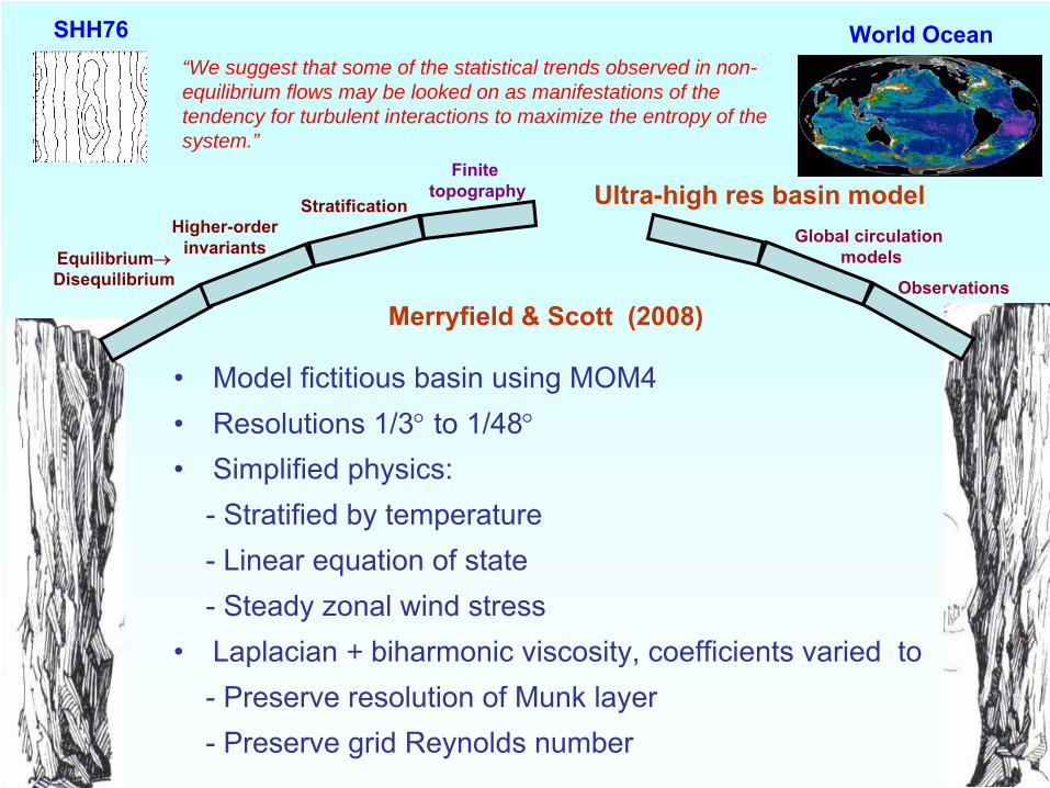
SHH76 World Ocean“We suggest that some of the statistical trends observed in non- equilibrium flows may be looked on as manifestations of the tendency for turbulent interactions to maximize the entropy of the system.”
Equilibrium→Disequilibrium
Higher-orderinvariants
Stratification
Finite topography
Observations
Global circulation models
Merryfield & Scott (2008)
Ultra-high res basin model
•
Model fictitious basin using MOM4•
Resolutions 1/3°
to 1/48°•
Simplified physics:-
Stratified by temperature-
Linear equation of state-
Steady zonal wind stress•
Laplacian
+ biharmonic
viscosity, coefficients varied to -
Preserve resolution of Munk
layer-
Preserve grid Reynolds number
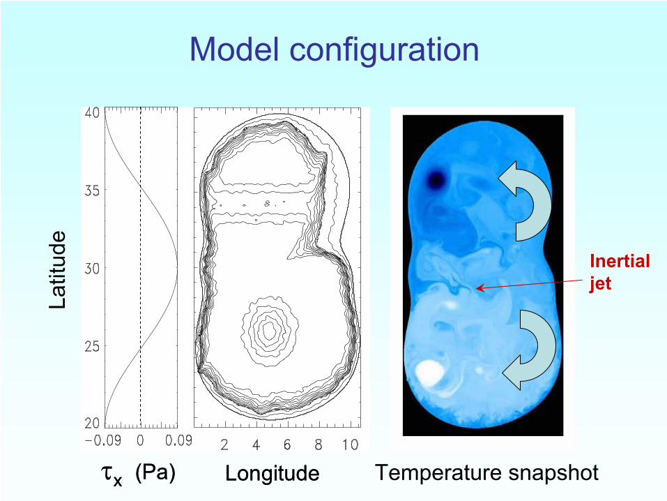
Model configuration
τx Longitude(Pa)τx Longitude(Pa)
Latit
ude
Temperature snapshot
Inertialjet
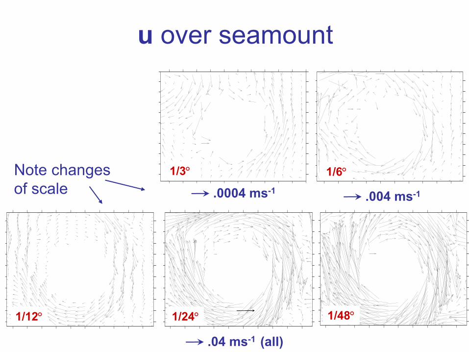
��
u
over seamount
1/3° 1/6°
1/12° 1/24° 1/48°
Note changes of scale .0004 ms-1 .004 ms-1
.04 ms-1 (all)
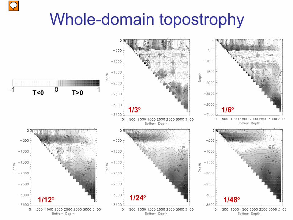
1/3° 1/6°
1/12° 1/24° 1/48°
-1 0 1T<0 T>0
Whole-domain topostrophy
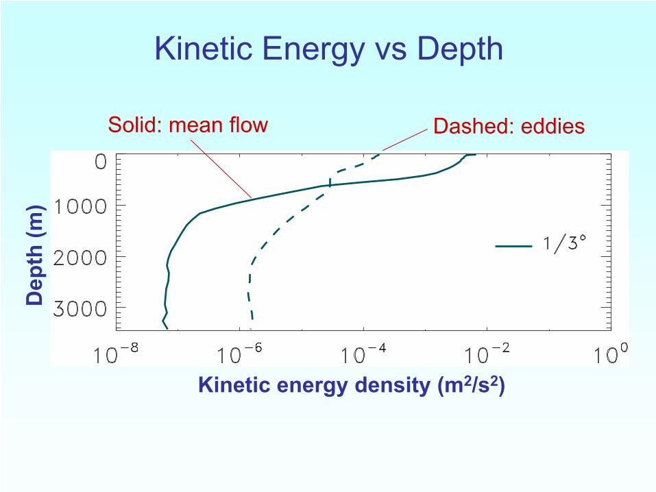
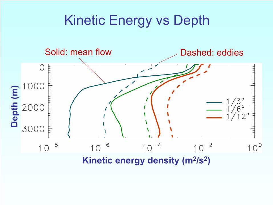
Kinetic Energy vs
DepthD
epth
(m)
Kinetic energy density (m2/s2)
Solid: mean flow Dashed: eddies
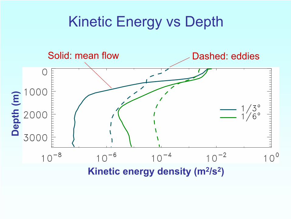
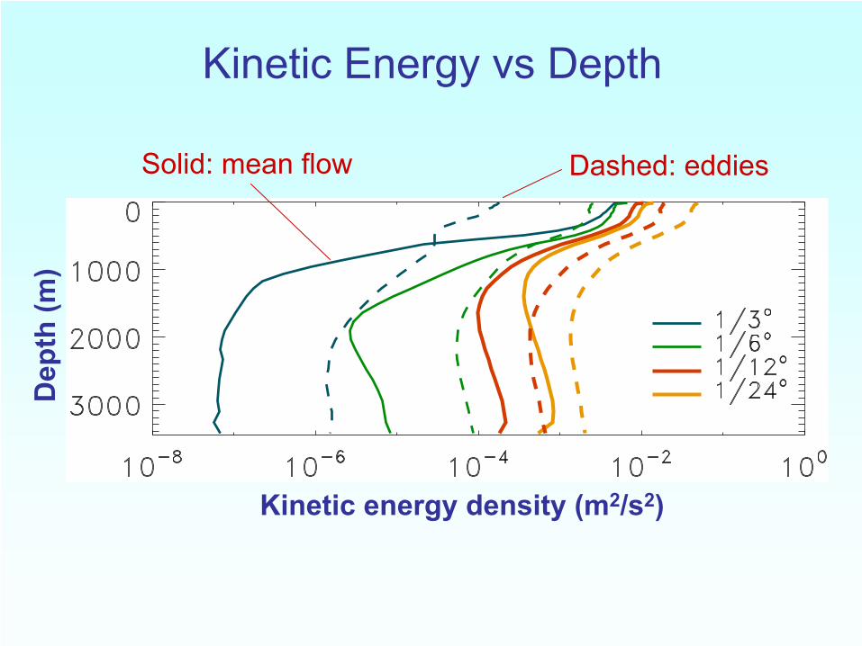
Kinetic Energy vs
DepthD
epth
(m)
Kinetic energy density (m2/s2)
Solid: mean flow Dashed: eddies
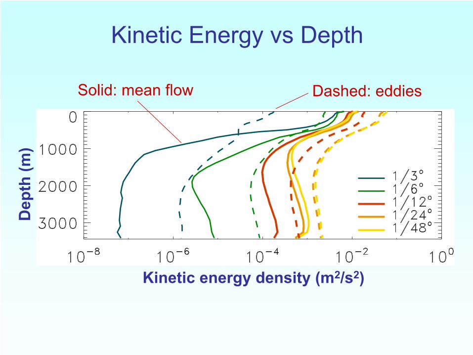
Kinetic Energy vs
DepthD
epth
(m)
Kinetic energy density (m2/s2)
Solid: mean flow Dashed: eddies
Kinetic Energy vs
DepthD
epth
(m)
Kinetic energy density (m2/s2)
Solid: mean flow Dashed: eddies
Kinetic Energy vs
DepthD
epth
(m)
Kinetic energy density (m2/s2)
Solid: mean flow Dashed: eddies
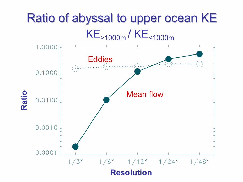
Ratio of abyssal to upper ocean KERatio of abyssal to upper ocean KE
Resolution
Eddies
Rat
io Mean flow
KE>1000m / KE<1000m
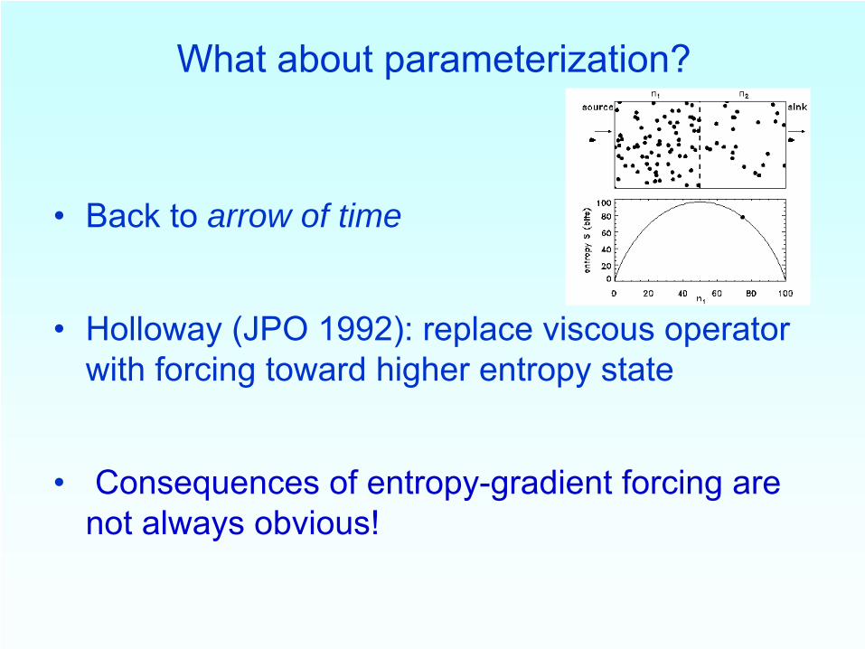
What about parameterization?
•
Back to arrow of time
•
Holloway (JPO 1992): replace viscous operator with forcing toward higher entropy state
•
Consequences of entropy-gradient forcing are not always obvious!
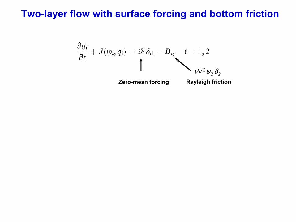
ν∇2ψ2 δ2
Rayleigh frictionZero-mean forcing
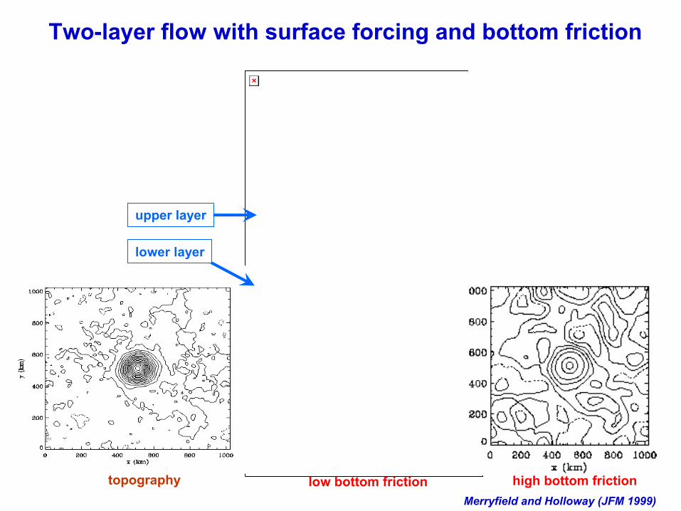
Two-layer flow with surface forcing and bottom friction
Merryfield and Holloway (JFM 1999)topography
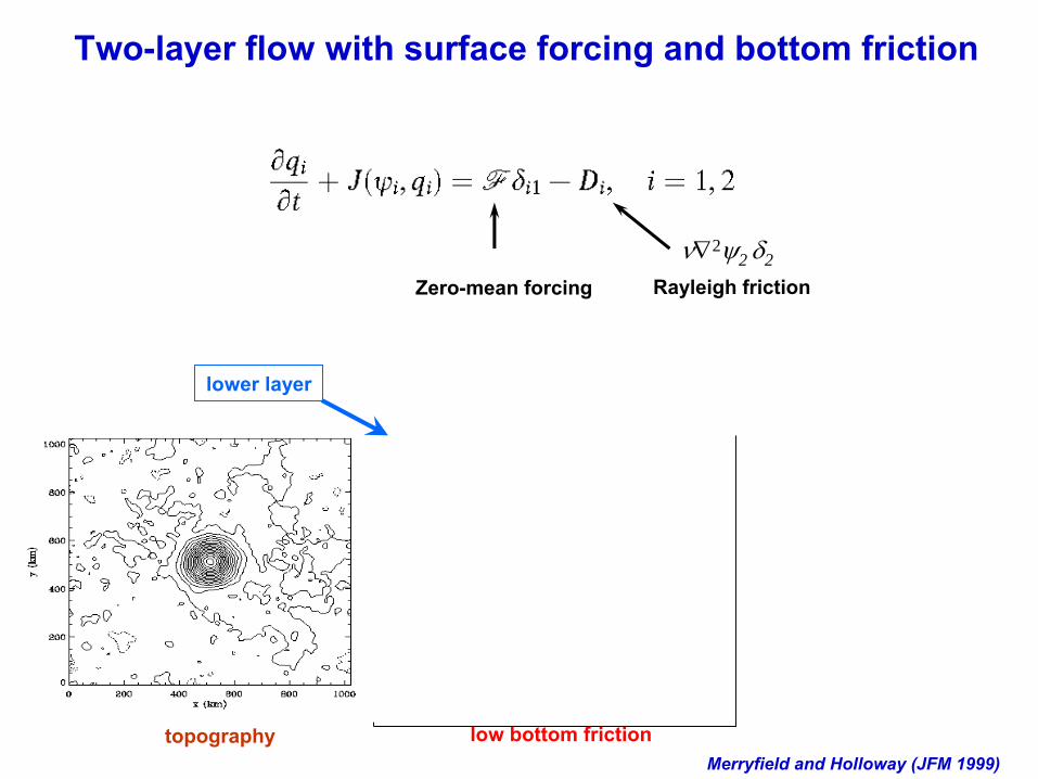
Two-layer flow with surface forcing and bottom friction
lower layerupper layer
low bottom friction
ν∇2ψ2 δ2
Rayleigh frictionZero-mean forcing
Merryfield and Holloway (JFM 1999)
topography
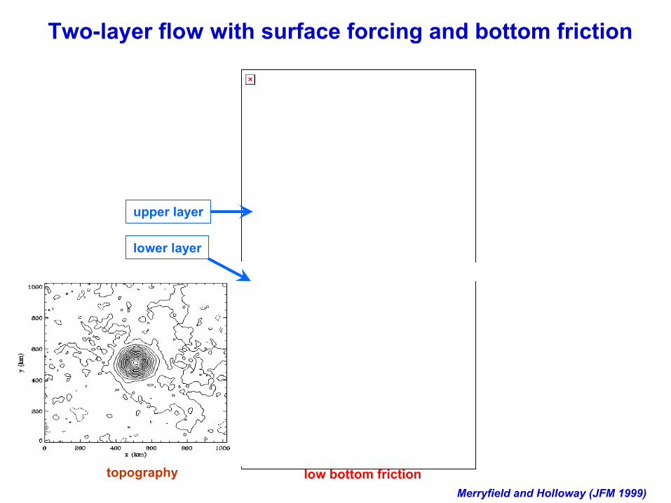
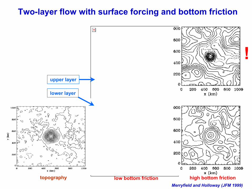
Two-layer flow with surface forcing and bottom friction
lower layer
upper layer
low bottom friction
high bottom frictionMerryfield and Holloway (JFM 1999)
topography
Two-layer flow with surface forcing and bottom friction
lower layer
upper layer
low bottom friction
Merryfield and Holloway (JFM 1999)
topography
Two-layer flow with surface forcing and bottom friction
!
low bottom friction
lower layer
upper layer
high bottom friction
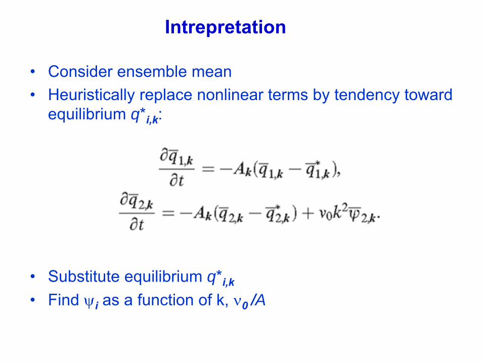
Intrepretation
•
Consider ensemble mean •
Heuristically replace nonlinear terms by tendency toward equilibrium q*i,k
:
•
Substitute equilibrium q*i,k
•
Find ψi
as a function of k, ν0 /A
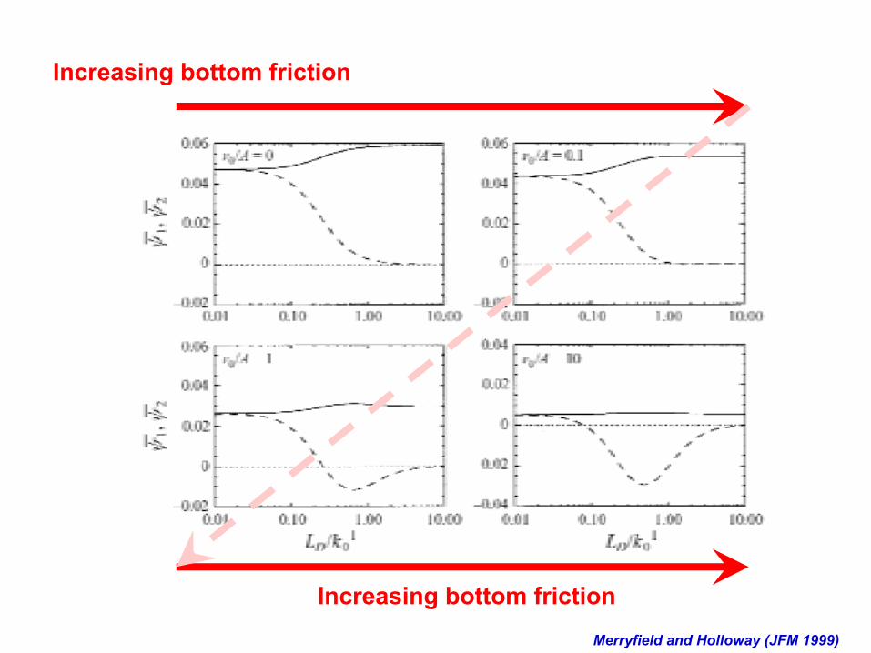
Merryfield and Holloway (JFM 1999)
Increasing bottom friction
Increasing bottom friction
Rectified flow over a seamount
Beckmann and Haidvogel
(JGR 1997)
SHH76 World Ocean“We suggest that some of the statistical trends observed in non- equilibrium flows may be looked on as manifestations of the tendency for turbulent interactions to maximize the entropy of the system.”
Equilibrium→Disequilibrium
Higher-orderinvariants
Stratification
Finite topography
Observations
Global circulation models
Ultra-high res basin model
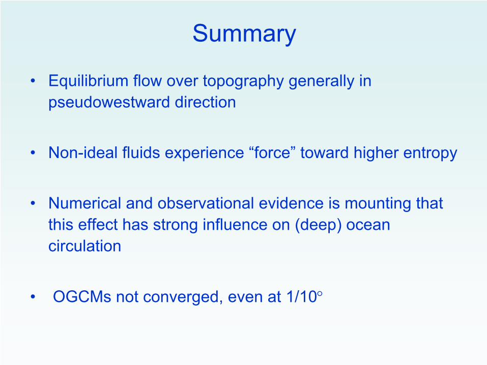
Summary
•
Equilibrium flow over topography generally in pseudowestward
direction
•
Non-ideal fluids experience “force”
toward higher entropy
•
Numerical and observational evidence is mounting that this effect has strong influence on (deep) ocean circulation
•
OGCMs
not converged, even at 1/10°
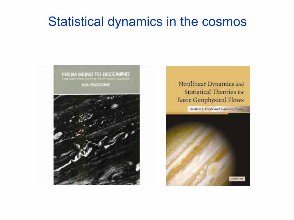
Statistical dynamics in the cosmos
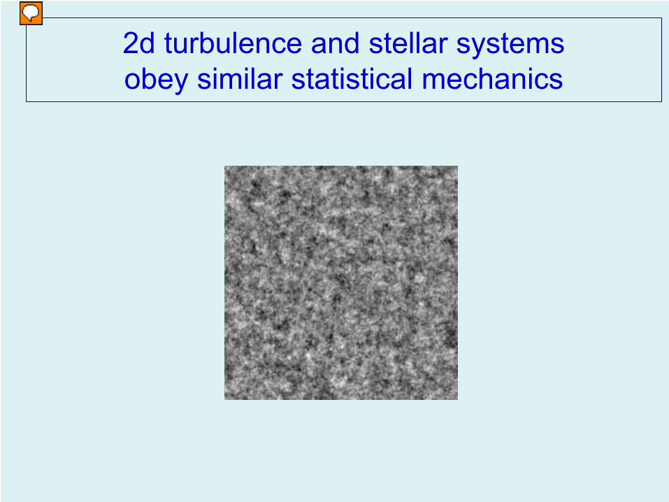
2d turbulence and stellar systems obey similar statistical mechanics
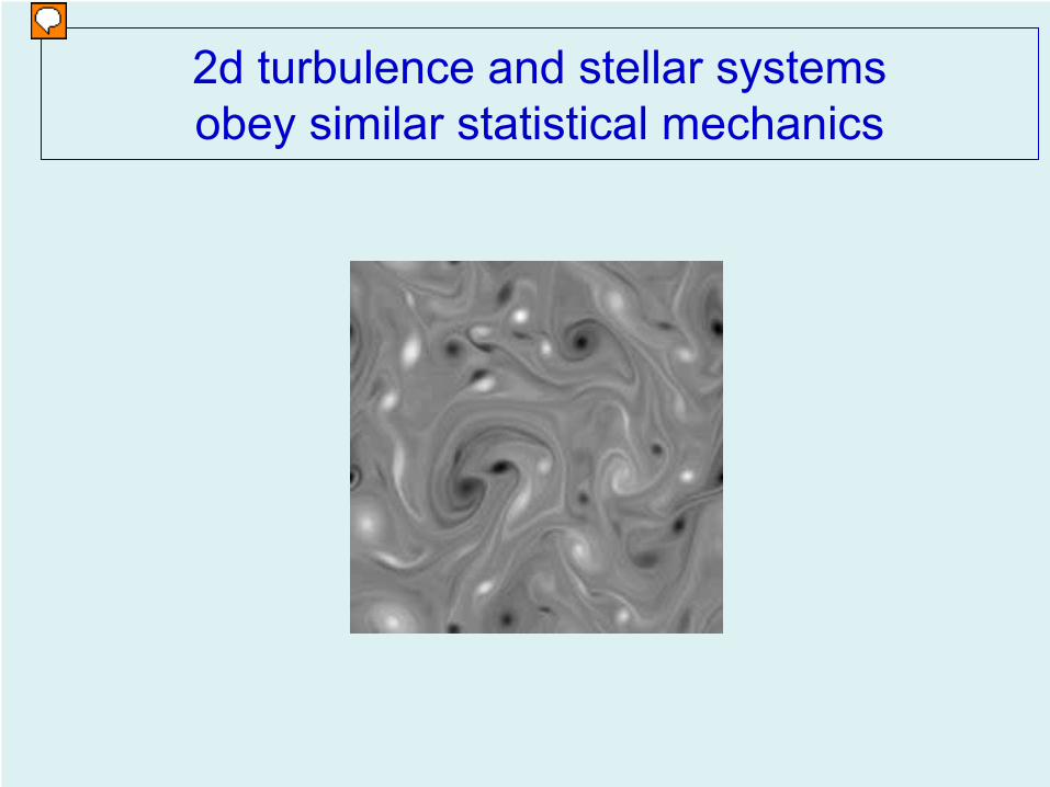
2d turbulence and stellar systems obey similar statistical mechanics
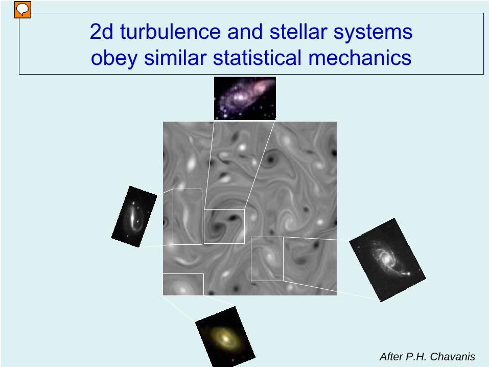
2d turbulence and stellar systems obey similar statistical mechanics
After P.H. Chavanis
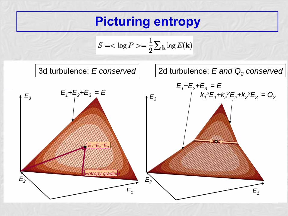
Picturing entropy
Σ
E1 =E2 =E3
E3 E3E1 +E2 +E3 = E
E1 +E2 +E3 = Ek1
2E1 +k22E2 +k3
2E3 = Q2
3d turbulence: E conserved 2d turbulence: E and Q2 conserved
Entropy gradient
E1
E2
E1
E2