Statistical Matching and Imputation of Survey Data with ... · Statistical matching techniques aim...

Statistical Matching and Imputation ofSurvey Data with StatMatch*

Marcello D’OrazioE-mail: [email protected]

January 9, 2017

1 Introduction

Statistical matching techniques aim at integrating two or more data sources (usuallydata from sample surveys) referred to the same target population. In the basic statisticalmatching framework, there are two data sources A and B sharing a set of variables Xwhile the variable Y is available only in A and the variable Z is observed just in B.The X variables are common to both the data sources, while the variables Y and Z arenot jointly observed. The objective of statistical matching (hereafter denoted as SM)consists in investigating the relationship between Y and Z at “micro” or “macro” level(D’Orazio et al., 2006b). In the micro case the SM aims at creating a “synthetic” datasource in which all the variables, X, Y and Z, are available (usually A ∪B with all themissing values filled in, or simply A filled in with the values of Z). When the objective ismacro, the data sources are integrated to derive an estimate of the parameter of interest,e.g. the correlation coefficient between Y and Z or the contingency table Y × Z.

A parametric approach to SM requires the explicit adoption of a model for (X,Y, Z);obviously, if the model is misspecified the results will not be reliable. The nonparametricapproach is more flexible in handling complex situations (different types of variables).The two approaches can be mixed: first a parametric model is assumed and its param-eters are estimated then a synthetic data set is derived through a nonparametric microapproach. In this manner the advantages of both parametric and nonparametric ap-proach are maintained: the model is parsimonious while nonparametric techniques offerprotection against model misspecification. Table 1 provides a summary of the objectivesand approaches to SM (D’Orazio et al., 2008).

*This document is partly based on the work carried out in the framework of the ESSnet project on DataIntegration, partly funded by Eurostat (December 2009–December 2011). For more information onthe project visit http://www.essnet-portal.eu/di/data-integration

1

mailto:[email protected]

http://www.essnet-portal.eu/di/data-integration

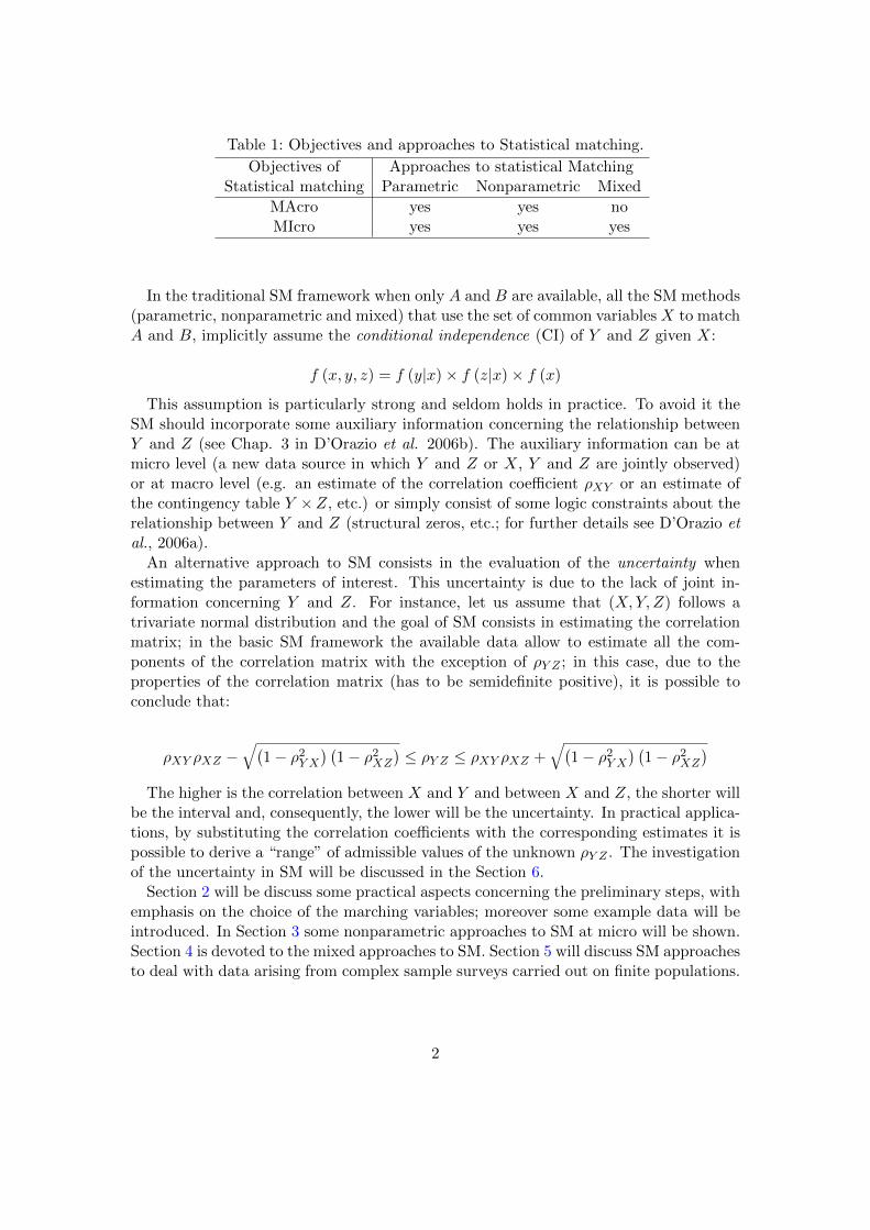
Table 1: Objectives and approaches to Statistical matching.

Objectives of Approaches to statistical MatchingStatistical matching Parametric Nonparametric Mixed

MAcro yes yes noMIcro yes yes yes

In the traditional SM framework when only A and B are available, all the SM methods(parametric, nonparametric and mixed) that use the set of common variables X to matchA and B, implicitly assume the conditional independence (CI) of Y and Z given X:

f (x, y, z) = f (y|x)× f (z|x)× f (x)

This assumption is particularly strong and seldom holds in practice. To avoid it theSM should incorporate some auxiliary information concerning the relationship betweenY and Z (see Chap. 3 in D’Orazio et al. 2006b). The auxiliary information can be atmicro level (a new data source in which Y and Z or X, Y and Z are jointly observed)or at macro level (e.g. an estimate of the correlation coefficient ρXY or an estimate ofthe contingency table Y ×Z, etc.) or simply consist of some logic constraints about therelationship between Y and Z (structural zeros, etc.; for further details see D’Orazio etal., 2006a).

An alternative approach to SM consists in the evaluation of the uncertainty whenestimating the parameters of interest. This uncertainty is due to the lack of joint in-formation concerning Y and Z. For instance, let us assume that (X,Y, Z) follows atrivariate normal distribution and the goal of SM consists in estimating the correlationmatrix; in the basic SM framework the available data allow to estimate all the com-ponents of the correlation matrix with the exception of ρY Z ; in this case, due to theproperties of the correlation matrix (has to be semidefinite positive), it is possible toconclude that:

ρXY ρXZ −√(

1− ρ2Y X

) (1− ρ2XZ

)≤ ρY Z ≤ ρXY ρXZ +

√(1− ρ2Y X

) (1− ρ2XZ

)The higher is the correlation between X and Y and between X and Z, the shorter will

be the interval and, consequently, the lower will be the uncertainty. In practical applica-tions, by substituting the correlation coefficients with the corresponding estimates it ispossible to derive a “range” of admissible values of the unknown ρY Z . The investigationof the uncertainty in SM will be discussed in the Section 6.

Section 2 will be discuss some practical aspects concerning the preliminary steps, withemphasis on the choice of the marching variables; moreover some example data will beintroduced. In Section 3 some nonparametric approaches to SM at micro will be shown.Section 4 is devoted to the mixed approaches to SM. Section 5 will discuss SM approachesto deal with data arising from complex sample surveys carried out on finite populations.

2

2 Practical steps in an application of statistical matching

Before applying SM methods in order to integrate two or more data sources some de-cisions and preprocessing steps are required (Scanu, 2008). In practice, given two datasources A and B related to the same target population, the following steps are necessary:

1. Choice of the target variables Y and Z, i.e. of the variables observed distinctly intwo sample surveys.

2. Identification of all the common variables X shared by A and B. In this step someharmonization procedures may be required because of different definitions and/orclassifications. Obviously, if two similar variables can not be harmonized they haveto be discarded. The common variables should not present missing values and theobserved values should be accurate (no measurement errors). Note that if A andB are representative samples of the same population then the common variablesare expected to share the same marginal/joint distribution.

3. Potentially all the X variables can be used directly in the SM application, so calledmatching variables but actually, not all them are used. Section 2.2 will providemore details concerning this issue.

4. The choice of the matching variables is strictly related to the matching framework(see Table 1).

5. Once decided the framework, a SM technique is used to match the samples.

6. Finally the results of the matching should be evaluated.

2.1 Example data

The next Sections will provide simple examples of application of some SM techniques inthe R environment (R Core Team, 2015) by using the functions in StatMatch (D’Orazio,2016). These examples will use artificial data set that come with StatMatch; theseartificial data sets are generated by considering the variables usually observed in theEU-SILC (European Union Statistics on Income and Living Conditions) survey (formajor details see StatMatch help pages).

> library(StatMatch) #loads pkg StatMatch

> data(samp.A) # sample A in SM examples

> str(samp.A)

'data.frame': 3009 obs. of 13 variables:

$ HH.P.id : chr "10149.01" "17154.02" "5628.01" "15319.01" ...

$ area5 : Factor w/ 5 levels "NE","NO","C",..: 1 1 2 4 4 3 4 5 4 3 ...

$ urb : Factor w/ 3 levels "1","2","3": 1 1 2 1 2 2 2 2 2 2 ...

$ hsize : int 1 2 1 2 5 2 4 3 4 4 ...

$ hsize5 : Factor w/ 5 levels "1","2","3","4",..: 1 2 1 2 5 2 4 3 4 4 ...

3

$ age : num 85 78 48 78 17 28 26 51 60 21 ...

$ c.age : Factor w/ 5 levels "[16,34]","(34,44]",..: 5 5 3 5 1 1 1 3 4 1 ...

$ sex : Factor w/ 2 levels "1","2": 2 1 1 1 1 2 2 2 2 2 ...

$ marital : Factor w/ 3 levels "1","2","3": 3 2 3 2 1 2 1 2 2 1 ...

$ edu7 : Factor w/ 7 levels "0","1","2","3",..: 4 4 4 2 2 6 6 3 2 4 ...

$ n.income: num 1677 13520 20000 12428 0 ...

$ c.neti : Factor w/ 7 levels "(-Inf,0]","(0,10]",..: 2 3 4 3 1 1 2 3 1 1 ...

$ ww : num 3592 415 2735 1240 5363 ...

> data(samp.B) # sample B in the SM examples

> str(samp.B)


$ HH.P.id: chr "5.01" "5.02" "24.01" "24.02" ...



$ hsize : int 2 2 2 2 2 2 3 3 3 3 ...


$ age : num 45 18 76 74 47 46 53 55 21 53 ...



$ marital: Factor w/ 3 levels "1","2","3": 3 1 2 2 1 1 2 2 1 2 ...


$ labour5: Factor w/ 5 levels "1","2","3","4",..: 3 5 4 4 1 5 5 1 5 1 ...

$ ww : num 179 179 330 330 1116 ...

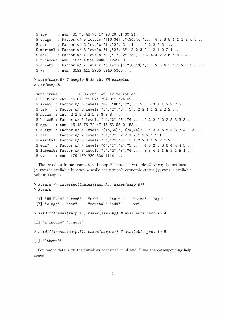
The two data frames samp.A and samp.B share the variables X.vars; the net income(z.var) is available in samp.A while the person’s economic status (y.var) is availableonly in samp.B.

> X.vars <- intersect(names(samp.A), names(samp.B))

> X.vars

[1] "HH.P.id" "area5" "urb" "hsize" "hsize5" "age"

[7] "c.age" "sex" "marital" "edu7" "ww"

> setdiff(names(samp.A), names(samp.B)) # available just in A

[1] "n.income" "c.neti"

> setdiff(names(samp.B), names(samp.A)) # available just in B

[1] "labour5"

For major details on the variables contained in A and B see the corresponding helppages.

4

2.2 The choice of the matching variables

In statistical matching applications A and B may share many common variables. Inpractice, just the most relevant ones, called matching variables, are used in the match-ing. The selection of these variables should be performed through opportune statisticalmethods (descriptive, inferential, etc.) and by consulting subject matter experts.

From a statistical point of view, the choice of the marching variables XM (XM ⊆ X)should be carried out in a “multivariate sense” in order to identify the subset of theXM variables connected at the same time with Y and Z (Cohen, 1991); unfortunatelythis would require the availability of an auxiliary data source in which all the variables(X,Y, Z) are observed. In the basic SM framework the data in A permit to explorethe relationship between Y and X, while the relationship between Z and X can beinvestigated in B. Then the results of the two separate analyses have to be combined insome manner; usually the subset of the matching variables is obtained as XM = XY ∪XZ ,being XY (XY ⊆ X) the subset of the common variables that better explains Y , whileXZ is the subset of the common variables that better explain Z (XZ ⊆ X). The risk isthat of ending with too many matching variables, thereby increasing the complexity ofthe problem and potentially affecting negatively the results of SM. In particular, in themicro approach this may introduce additional undesired variability and bias as far asthe joint (marginal) distribution of XM and Z is concerned. For this reason sometimesthe set of the matching variables is obtained as a compromise

XY ∩XZ ⊆ XM ⊆ XY ∪XZ

.The simplest procedure to identify XY consists in calculation of pairwise correla-

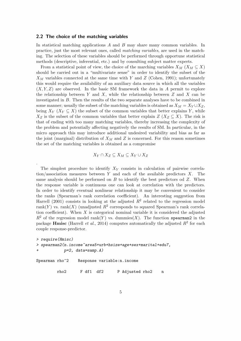
tion/association measures between Y and each of the available predictors X. Thesame analysis should be performed on B to identify the best predictors od Z. Whenthe response variable is continuous one can look at correlation with the predictors.In order to identify eventual nonlinear relationship it may be convenient to considerthe ranks (Spearman’s rank correlation coefficient). An interesting suggestion fromHarrell (2001) consists in looking at the adjusted R2 related to the regression modelrank(Y ) vs. rank(X) (unadjusted R2 corresponds to squared Spearman’s rank correla-tion coefficient). When X is categorical nominal variable it is considered the adjustedR2 of the regression model rank(Y ) vs. dummies(X). The function spearman2 in thepackage Hmisc (Harrell et al., 2014) computes automatically the adjusted R2 for eachcouple response-predictor.

> require(Hmisc)

> spearman2(n.income~area5+urb+hsize+age+sex+marital+edu7,

+ p=2, data=samp.A)

Spearman rho^2 Response variable:n.income

rho2 F df1 df2 P Adjusted rho2 n

5

area5 0.033 25.45 4 3004 0.0000 0.031 3009

urb 0.000 0.49 2 3006 0.6105 0.000 3009

hsize 0.032 49.82 2 3006 0.0000 0.031 3009

age 0.136 236.99 2 3006 0.0000 0.136 3009

sex 0.120 410.25 1 3007 0.0000 0.120 3009

marital 0.034 53.02 2 3006 0.0000 0.033 3009

edu7 0.071 38.17 6 3002 0.0000 0.069 3009

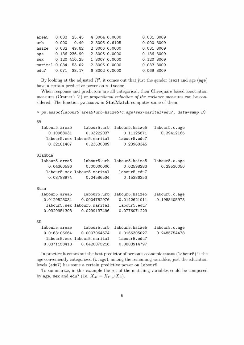
By looking at the adjusted R2, it comes out that just the gender (sex) and age (age)have a certain predictive power on n.income.

When response and predictors are all categorical, then Chi-square based associationmeasures (Cramer’s V ) or proportional reduction of the variance measures can be con-sidered. The function pw.assoc in StatMatch computes some of them.

> pw.assoc(labour5~area5+urb+hsize5+c.age+sex+marital+edu7, data=samp.B)

$V

labour5.area5 labour5.urb labour5.hsize5 labour5.c.age

0.10968031 0.03222037 0.11125871 0.39412166

labour5.sex labour5.marital labour5.edu7

0.32181407 0.23630089 0.23968345

$lambda


0.04360596 0.00000000 0.02598283 0.29530050


0.08788974 0.04586534 0.15386353

$tau


0.0129525034 0.0004782976 0.0142621011 0.1988405973


0.0329951308 0.0299137496 0.0776071229

$U


0.0163106664 0.0007064674 0.0166305027 0.2485754478


0.0371158413 0.0420075216 0.0803914797

In practice it comes out the best predictor of person’s economic status (labour5) is theage conveniently categorized (c.age), among the remaining variables, just the educationlevels (edu7) has some a certain predictive power on labour5.

To summarize, in this example the set of the matching variables could be composedby age, sex and edu7 (i.e. XM = XY ∪XZ).

6

When too many variables are available, before computing pairwise association/correlationmeasures it would be necessary to discard the redundant predictors (functions redun andvarclus in Hmisc can be of help).

Sometimes the important predictors can be identified by fitting models and then run-ning procedures for selecting the best predictors. The selection of the subset XY can alsobe demanded to nonparametric procedures such as Classification And Regression Trees(Breiman et al., 1984). Instead of fitting a single tree, it would be better to fit a randomforest (Breiman, 2001) by means of the function randomForest available in the packagerandomForest (Liaw and Wiener, 2002) which provides a measure of importance forthe predictors (to be used with caution).

The approach to SM based on the study of uncertainty offers the possibility of choosingthe matching variable by selecting just those common variables with the highest contri-bution to the reduction of the uncertainty. The function Fbwidths.by.x in StatMatchpermits to explore the reduction of uncertainty when all the variables (X,Y, Z) are cat-egorical. In particular, assuming that XD correspond to the complete crossing of thematching variables XM , it is possible to show that in the basic SM framework

P(low)j,k ≤ PY=j,Z=k ≤ P

(up)j,k ,

being

P(low)j,k =

∑i

PXD=i ×max{

0;PY=j|XD=i + PZ=k|XD=i − 1}

P(up)j,k =

∑i

PXD=i ×min{PY=j|XD=i;PZ=k|XD=i

}for j = 1, . . . , J and k = 1, . . . ,K, being J and K the categories of Y and Z respectively.

The function Fbwidths.by.x estimates (P(low)j,k , P

(up)j,k ) for each cell in the contingency

table Y ×Z for all the possible combinations of the input X variables; then the reductionof uncertainty is measured naively by the average widths of the intervals:

d =1

J ×K∑j,k

(P(up)j,k − P

(low)j,k )

> # choiche of the matching variables based on uncertainty

> xx <- xtabs(~c.age+sex+marital+edu7, data=samp.A)

> xy <- xtabs(~c.age+sex+marital+edu7+c.neti, data=samp.A)

> xz <- xtabs(~c.age+sex+marital+edu7+labour5, data=samp.B)

> out.fbw <- Fbwidths.by.x(tab.x=xx, tab.xy=xy, tab.xz=xz)

> # sort output according to average width

> sort.av <- out.fbw$sum.unc[order(out.fbw$sum.unc$av.width),]

> head(sort.av) # best 6 combinations of the Xs

x.vars x.cells x.freq0 xy.cells xy.freq0

|c.age*sex*marital*edu7 4 210 51 1470 863

7

|c.age*sex*edu7 3 70 7 490 168

|c.age*sex*marital 3 30 0 210 18

|c.age*marital*edu7 3 105 16 735 341

|c.age*sex 2 10 0 70 0

|c.age*edu7 2 35 1 245 55

xz.cells xz.freq0 av.width rel.av.width

|c.age*sex*marital*edu7 1050 538 0.06598348 0.5688524

|c.age*sex*edu7 350 111 0.07158300 0.6171266

|c.age*sex*marital 150 22 0.07559817 0.6517420

|c.age*marital*edu7 525 213 0.07760632 0.6690545

|c.age*sex 50 3 0.07804262 0.6728159

|c.age*edu7 175 42 0.08114008 0.6995195

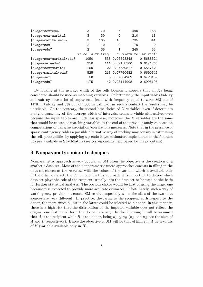
By looking at the average width of the cells bounds it appears that all Xs beingconsidered should be used as matching variables. Unfortunately the input tables tab.xyand tab.xy have a lot of empty cells (cells with frequency equal to zero; 863 out of1470 in tab.xy and 538 out of 1050 in tab.xy); in such a context the results may beunreliable. On the contrary, the second best choice of X variables, even if determinesa slight worsening of the average width of intervals, seems a viable alternative, evenbecause the input tables are much less sparse; moreover the X variables are the samethat would be chosen as matching variables at the end of the previous analyses based oncomputations of pairwise association/correlations measures. Note that in the presence ofsparse contingency tables a possible alternative way of working may consist in estimatingthe cells probabilities by applying a pseudo-Bayes estimator, implemented in the functionpBayes available in StatMatch (see corresponding help pages for major details).

3 Nonparametric micro techniques

Nonparametric approach is very popular in SM when the objective is the creation of asynthetic data set. Most of the nonparametric micro approaches consists in filling in thedata set chosen as the recipient with the values of the variable which is available onlyin the other data set, the donor one. In this approach it is important to decide whichdata set plays the role of the recipient; usually it is the data set to be used as the basisfor further statistical analyses. The obvious choice would be that of using the larger onebecause it is expected to provide more accurate estimates; unfortunately, such a way ofworking may provide inaccurate SM results, especially when the sizes of the two datasources are very different. In practice, the larger is the recipient with respect to thedonor, the more times a unit in the latter could be selected as a donor. In this manner,there is a high risk that the distribution of the imputed variable does not reflect theoriginal one (estimated form the donor data set). In the following it will be assumedthat A is the recipient while B is the donor, being nA ≤ nB (nA and nB are the sizes ofA and B respectively). Hence the objective of SM will be that of filling in A with valuesof Y (variable available only in B).

8

In StatMatch the following nonparametric micro techniques are available: randomhot deck, nearest neighbor hot deck and rank hot deck (see Section 2.4 in D’Orazio et al.,2006b; Singh et al., 1993).

3.1 Nearest neighbor distance hot deck

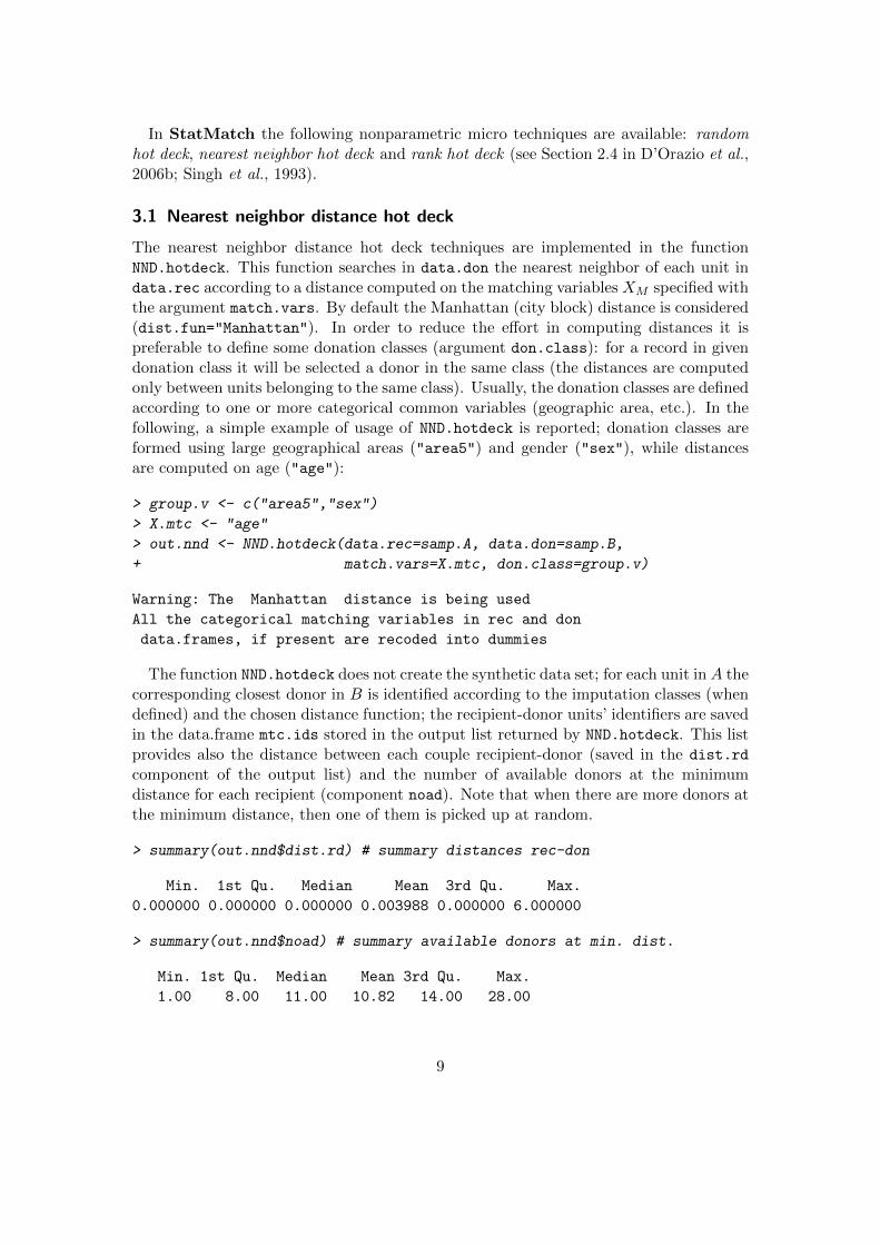
The nearest neighbor distance hot deck techniques are implemented in the functionNND.hotdeck. This function searches in data.don the nearest neighbor of each unit indata.rec according to a distance computed on the matching variables XM specified withthe argument match.vars. By default the Manhattan (city block) distance is considered(dist.fun="Manhattan"). In order to reduce the effort in computing distances it ispreferable to define some donation classes (argument don.class): for a record in givendonation class it will be selected a donor in the same class (the distances are computedonly between units belonging to the same class). Usually, the donation classes are definedaccording to one or more categorical common variables (geographic area, etc.). In thefollowing, a simple example of usage of NND.hotdeck is reported; donation classes areformed using large geographical areas ("area5") and gender ("sex"), while distancesare computed on age ("age"):

> group.v <- c("area5","sex")

> X.mtc <- "age"

> out.nnd <- NND.hotdeck(data.rec=samp.A, data.don=samp.B,

+ match.vars=X.mtc, don.class=group.v)

Warning: The Manhattan distance is being used

All the categorical matching variables in rec and don

data.frames, if present are recoded into dummies

The function NND.hotdeck does not create the synthetic data set; for each unit in A thecorresponding closest donor in B is identified according to the imputation classes (whendefined) and the chosen distance function; the recipient-donor units’ identifiers are savedin the data.frame mtc.ids stored in the output list returned by NND.hotdeck. This listprovides also the distance between each couple recipient-donor (saved in the dist.rd

component of the output list) and the number of available donors at the minimumdistance for each recipient (component noad). Note that when there are more donors atthe minimum distance, then one of them is picked up at random.

> summary(out.nnd$dist.rd) # summary distances rec-don

Min. 1st Qu. Median Mean 3rd Qu. Max.

0.000000 0.000000 0.000000 0.003988 0.000000 6.000000

> summary(out.nnd$noad) # summary available donors at min. dist.


1.00 8.00 11.00 10.82 14.00 28.00

9

In order to derive the synthetic data set it is necessary to run the function cre-

ate.fused which requires the output of NND.hotdeck function (component mtc.ids ofthe output’s list) and the specification of the Z variables to donate from B to A via theargument z.vars:

> head(out.nnd$mtc.ids)

rec.id don.id

[1,] "35973" "27403"

[2,] "21483" "36572"

[3,] "39095" "29030"

[4,] "36844" "22421"

[5,] "560" "33394"

[6,] "34062" "13754"

> fA.nnd <- create.fused(data.rec=samp.A, data.don=samp.B,

+ mtc.ids=out.nnd$mtc.ids,

+ z.vars="labour5")

> head(fA.nnd) #first 6 obs.

HH.P.id area5 urb hsize hsize5 age c.age sex marital

35973 17154.02 NE 1 2 2 78 (64,104] 1 2

21483 10198.01 NE 2 1 1 54 (44,54] 1 2

39095 18619.02 NE 1 2 2 42 (34,44] 1 1

36844 17559.01 NE 2 2 2 55 (54,64] 1 2

560 260.01 NE 2 2 2 70 (64,104] 1 2

34062 16246.01 NE 2 3 3 66 (64,104] 1 2

edu7 n.income c.neti ww labour5

35973 3 13520 (10,15] 415.1592 4

21483 3 0 (-Inf,0] 985.7281 1

39095 2 18937 (15,20] 5728.2815 1

36844 2 18666 (15,20] 1592.5737 1

560 1 8619 (0,10] 2163.1869 4

34062 3 21268 (20,25] 1970.7038 4

As far as distances are concerned (argument dist.fun), all the distance functions inthe package proxy (Meyer and Butchta, 2015) are available. Anyway, for some partic-ular distances it was decided to write specific R functions. In particular, when dealingwith continuous matching variables it is possible to use the maximum distance (L∞

norm) implemented in maximum.dist; this function works on the true observed values(continuous variables) or on transformed ranked values (argument rank=TRUE) as sug-gested in Kovar et al. (1988); the transformation (ranks divided by the number of units)removes the effect of different scales and the new values are uniformly distributed in theinterval [0, 1]. The Mahalanobis distance can be computed by using mahalanobis.dist

10

which allows an external estimate of the covariance matrix (argument vc). When deal-ing with mixed type matching variables, the Gowers’s dissimilarity (Gower, 1981) canbe computed (function gower.dist): it is an average of the distances computed on thesingle variables according to different rules, depending on the type of the variable. Allthe distances are scaled to range from 0 to 1, hence the overall distance cat take a valuein [0, 1]. When dealing with mixed types matching variables it is still possible to usethe distance functions for continuous variables but NND.hotdeck transforms factors intodummies (by means of the function fact2dummy).

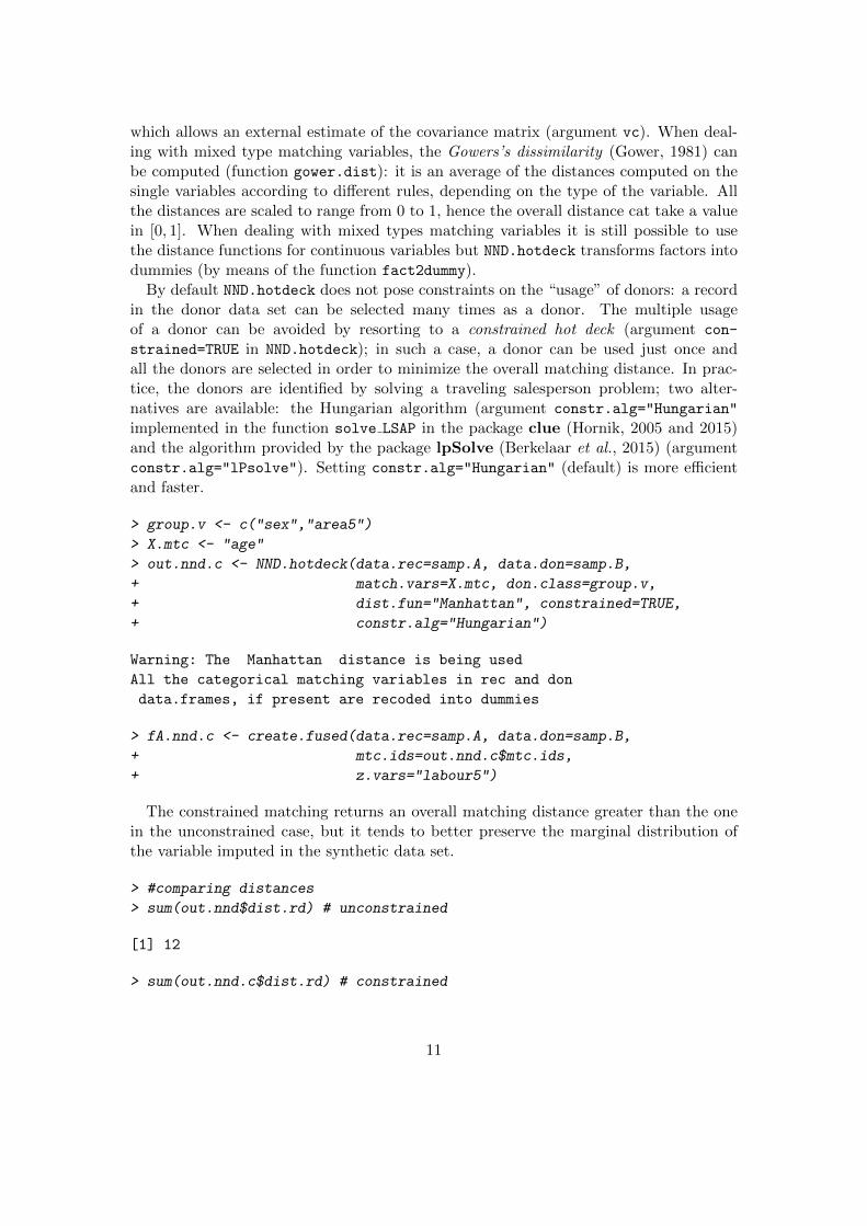
By default NND.hotdeck does not pose constraints on the “usage” of donors: a recordin the donor data set can be selected many times as a donor. The multiple usageof a donor can be avoided by resorting to a constrained hot deck (argument con-

strained=TRUE in NND.hotdeck); in such a case, a donor can be used just once andall the donors are selected in order to minimize the overall matching distance. In prac-tice, the donors are identified by solving a traveling salesperson problem; two alter-natives are available: the Hungarian algorithm (argument constr.alg="Hungarian"

implemented in the function solve LSAP in the package clue (Hornik, 2005 and 2015)and the algorithm provided by the package lpSolve (Berkelaar et al., 2015) (argumentconstr.alg="lPsolve"). Setting constr.alg="Hungarian" (default) is more efficientand faster.

> group.v <- c("sex","area5")

> X.mtc <- "age"

> out.nnd.c <- NND.hotdeck(data.rec=samp.A, data.don=samp.B,

+ match.vars=X.mtc, don.class=group.v,

+ dist.fun="Manhattan", constrained=TRUE,

+ constr.alg="Hungarian")




> fA.nnd.c <- create.fused(data.rec=samp.A, data.don=samp.B,

+ mtc.ids=out.nnd.c$mtc.ids,

+ z.vars="labour5")

The constrained matching returns an overall matching distance greater than the onein the unconstrained case, but it tends to better preserve the marginal distribution ofthe variable imputed in the synthetic data set.

> #comparing distances

> sum(out.nnd$dist.rd) # unconstrained

[1] 12

> sum(out.nnd.c$dist.rd) # constrained

11

[1] 90

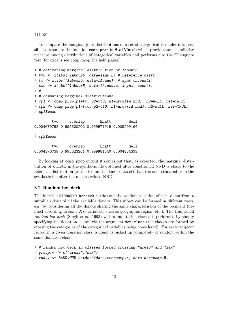
To compare the marginal joint distributions of a set of categorical variables it is pos-sible to resort to the function comp.prop in StatMatch which provides some similaritymeasure among distributions of categorical variables and performs also the Chi-squaretest (for details see comp.prop the help pages).

> # estimating marginal distribution of labour5

> tt0 <- xtabs(~labour5, data=samp.B) # reference distr.

> tt <- xtabs(~labour5, data=fA.nnd) # synt unconstr.

> ttc <- xtabs(~labour5, data=fA.nnd.c) #synt. constr.

> #

> # comparing marginal distributions

> cp1 <- comp.prop(p1=tt, p2=tt0, n1=nrow(fA.nnd), n2=NULL, ref=TRUE)

> cp2 <- comp.prop(p1=ttc, p2=tt0, n1=nrow(fA.nnd), n2=NULL, ref=TRUE)

> cp1$meas

tvd overlap Bhatt Hell

0.004679798 0.995320202 0.999971919 0.005299164

> cp2$meas


0.004376739 0.995623261 0.999981040 0.004354333

By looking at comp.prop output it comes out that, as expected, the marginal distri-bution of c.netI in the synthetic file obtained after constrained NND is closer to thereference distribution (estimated on the donor dataset) than the one estimated from thesynthetic file after the unconstrained NND.

3.2 Random hot deck

The function RANDwNND.hotdeck carries out the random selection of each donor from asuitable subset of all the available donors. This subset can be formed in different ways,e.g. by considering all the donors sharing the same characteristics of the recipient (de-fined according to some XM variables, such as geographic region, etc.). The traditionalrandom hot deck (Singh et al., 1993) within imputation classes is performed by simplyspecifying the donation classes via the argument don.class (the classes are formed bycrossing the categories of the categorical variables being considered). For each recipientrecord in a given donation class, a donor is picked up completely at random within thesame donation class.

> # random hot deck in classes formed crossing "area5" and "sex"


> rnd.1 <- RANDwNND.hotdeck(data.rec=samp.A, data.don=samp.B,

12

+ match.vars=NULL, don.class=group.v)

> fA.rnd <- create.fused(data.rec=samp.A, data.don=samp.B,

+ mtc.ids=rnd.1$mtc.ids,

+ z.vars="labour5")

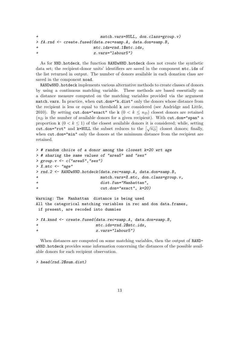
As for NND.hotdeck, the function RANDwNND.hotdeck does not create the syntheticdata set; the recipient-donor units’ identifiers are saved in the component mtc.ids ofthe list returned in output. The number of donors available in each donation class aresaved in the component noad.RANDwNND.hotdeck implements various alternative methods to create classes of donors

by using a continuous matching variable. These methods are based essentially ona distance measure computed on the matching variables provided via the argumentmatch.vars. In practice, when cut.don="k.dist" only the donors whose distance fromthe recipient is less or equal to threshold k are considered (see Andridge and Little,2010). By setting cut.don="exact" the k (0 < k ≤ nD) closest donors are retained(nD is the number of available donors for a given recipient). With cut.don="span" aproportion k (0 < k ≤ 1) of the closest available donors it is considered; while, settingcut.don="rot" and k=NULL the subset reduces to the

[√nD]

closest donors; finally,when cut.don="min" only the donors at the minimum distance from the recipient areretained.

> # random choice of a donor among the closest k=20 wrt age

> # sharing the same values of "area5" and "sex"


> X.mtc <- "age"


+ match.vars=X.mtc, don.class=group.v,

+ dist.fun="Manhattan",

+ cut.don="exact", k=20)


All the categorical matching variables in rec and don data.frames,

if present, are recoded into dummies

> fA.knnd <- create.fused(data.rec=samp.A, data.don=samp.B,


+ z.vars="labour5")

When distances are computed on some matching variables, then the output of RAND-wNND.hotdeck provides some information concerning the distances of the possible avail-able donors for each recipient observation.

> head(rnd.2$sum.dist)

13

min max sd cut dist.rd

[1,] 0 61 17.204128 1 0

[2,] 0 38 9.898723 1 1

[3,] 0 50 11.642050 1 0

[4,] 0 38 10.037090 1 1

[5,] 0 53 14.865282 1 0

[6,] 0 49 13.404280 1 1

In particular, "min", "max" and "sd" columns report respectively the minimum, themaximum and the standard deviation of the distances (all the available donors areconsidered), while "cut" refers to the distance of the kth closest donor; "dist.rd" isdistance existing among the recipient and the randomly chosen donor.

When selecting a donor among those available in the subset identified by the argumentscut.don and k, it is possible to use a weighted selection by specifying a weighting variablevia weight.don argument. This topic will be tackled in Section 5.

3.3 Rank hot deck

The rank hot deck distance method has been introduced by Singh et al. (1993). Itsearches for the donor at a minimum distance from the given recipient record but, inthis case, the distance is computed on the percentage points of the empirical cumulativedistribution function of the unique (continuous) common variable XM being considered.The empirical cumulative distribution function is estimated by:

F (x) =1

n

n∑i=1

I (xi ≤ x)

being I() = 1 if xi ≤ x and 0 otherwise. This transformation provides values uniformlydistributed in the interval [0, 1]; moreover, it can be useful when the values of XM cannot be directly compared because of measurement errors which however do not affectthe “position” of a unit in the whole distribution (D’Orazio et al., 2006b). This methodis implemented in the function rankNND.hotdeck. The following simple example showshow to call it.

> # distance computed on the percentage points of ecdf of "age"

> rnk.1 <- rankNND.hotdeck(data.rec=samp.A, data.don=samp.B,

+ var.rec="age", var.don="age")

> #create the synthetic data set

> fA.rnk <- create.fused(data.rec=samp.A, data.don=samp.B,

+ mtc.ids=rnk.1$mtc.ids,

+ z.vars="labour5",

+ dup.x=TRUE, match.vars="age")

> head(fA.rnk)


21384 10149.01 NE 1 1 1 85 (64,104] 2 3

14

35973 17154.02 NE 1 2 2 78 (64,104] 1 2

11774 5628.01 NO 2 1 1 48 (44,54] 1 3

32127 15319.01 S 1 2 2 78 (64,104] 1 2

6301 2973.05 S 2 5 >=5 17 [16,34] 1 1

12990 6206.02 C 2 2 2 28 [16,34] 2 2

edu7 n.income c.neti ww age.don labour5

21384 3 1677 (0,10] 3591.8939 85 4

35973 3 13520 (10,15] 415.1592 78 4

11774 3 20000 (15,20] 2735.4029 48 2

32127 1 12428 (10,15] 1239.5086 78 5

6301 1 0 (-Inf,0] 5362.7588 17 3

12990 5 0 (-Inf,0] 2077.7137 28 3

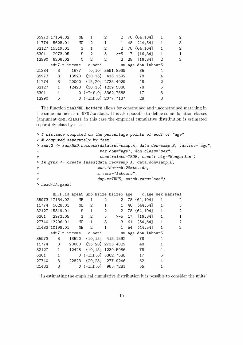
The function rankNND.hotdeck allows for constrained and unconstrained matching inthe same manner as in NND.hotdeck. It is also possible to define some donation classes(argument don.class), in this case the empirical cumulative distribution is estimatedseparately class by class.

> # distance computed on the percentage points of ecdf of "age"

> # computed separately by "sex"

> rnk.2 <- rankNND.hotdeck(data.rec=samp.A, data.don=samp.B, var.rec="age",

+ var.don="age", don.class="sex",

+ constrained=TRUE, constr.alg="Hungarian")

> fA.grnk <- create.fused(data.rec=samp.A, data.don=samp.B,

+ mtc.ids=rnk.2$mtc.ids,

+ z.vars="labour5",


> head(fA.grnk)


35973 17154.02 NE 1 2 2 78 (64,104] 1 2

11774 5628.01 NO 2 1 1 48 (44,54] 1 3

32127 15319.01 S 1 2 2 78 (64,104] 1 2

6301 2973.05 S 2 5 >=5 17 [16,34] 1 1

27740 13206.01 NO 1 3 3 61 (54,64] 1 2

21483 10198.01 NE 2 1 1 54 (44,54] 1 2

edu7 n.income c.neti ww age.don labour5

35973 3 13520 (10,15] 415.1592 78 4

11774 3 20000 (15,20] 2735.4029 48 1

32127 1 12428 (10,15] 1239.5086 78 4

6301 1 0 (-Inf,0] 5362.7588 17 5

27740 3 22823 (20,25] 277.9246 62 4

21483 3 0 (-Inf,0] 985.7281 55 1

In estimating the empirical cumulative distribution it is possible to consider the units’

15

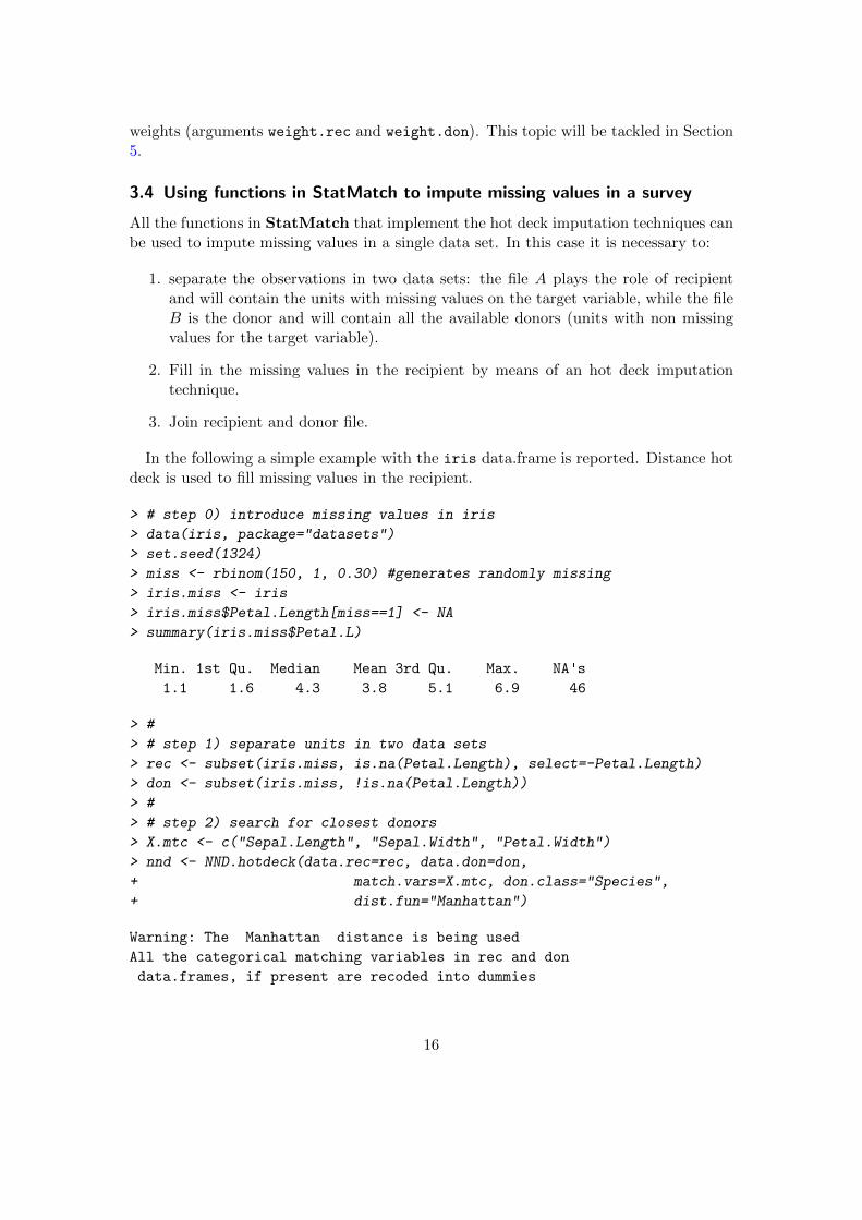
weights (arguments weight.rec and weight.don). This topic will be tackled in Section5.

3.4 Using functions in StatMatch to impute missing values in a survey

All the functions in StatMatch that implement the hot deck imputation techniques canbe used to impute missing values in a single data set. In this case it is necessary to:

1. separate the observations in two data sets: the file A plays the role of recipientand will contain the units with missing values on the target variable, while the fileB is the donor and will contain all the available donors (units with non missingvalues for the target variable).

2. Fill in the missing values in the recipient by means of an hot deck imputationtechnique.

3. Join recipient and donor file.

In the following a simple example with the iris data.frame is reported. Distance hotdeck is used to fill missing values in the recipient.

> # step 0) introduce missing values in iris

> data(iris, package="datasets")

> set.seed(1324)

> miss <- rbinom(150, 1, 0.30) #generates randomly missing

> iris.miss <- iris

> iris.miss$Petal.Length[miss==1] <- NA

> summary(iris.miss$Petal.L)

Min. 1st Qu. Median Mean 3rd Qu. Max. NA's

1.1 1.6 4.3 3.8 5.1 6.9 46

> #

> # step 1) separate units in two data sets

> rec <- subset(iris.miss, is.na(Petal.Length), select=-Petal.Length)

> don <- subset(iris.miss, !is.na(Petal.Length))

> #

> # step 2) search for closest donors

> X.mtc <- c("Sepal.Length", "Sepal.Width", "Petal.Width")

> nnd <- NND.hotdeck(data.rec=rec, data.don=don,

+ match.vars=X.mtc, don.class="Species",

+ dist.fun="Manhattan")




16

> # fills rec

> imp.rec <- create.fused(data.rec=rec, data.don=don,

+ mtc.ids=nnd$mtc.ids, z.vars="Petal.Length")

> imp.rec$imp.PL <- 1 # flag for imputed

> #

> # step 3) re-aggregate data sets

> don$imp.PL <- 0

> imp.iris <- rbind(imp.rec, don)

> #summary stat of imputed and non imputed Petal.Length

> tapply(imp.iris$Petal.Length, imp.iris$imp.PL, summary)

$`0`


1.1 1.6 4.3 3.8 5.1 6.9

$`1`


1.300 1.425 4.200 3.591 5.100 6.700

4 Mixed methods

A SM mixed method consists of two steps: (1) a model is fitted and all its parameters areestimated, then (2) a nonparametric approach is used to create the synthetic data set.The model is more parsimonious while the nonparametric approach offers “protection”against model misspecification. The implemented mixed approaches for SM are basedessentially on predictive mean matching imputation methods (see D’Orazio et al. 2006b,Section 2.5 and 3.6). In particular, the function mixed.mtc in StatMatch can use twosimilar mixed methods that manage variables (XM , Y, Z) following the the multivariatenormal distribution. The main difference is in step (1) when estimating the parametersof the two regressions Y vs. XM and Z vs. XM . By default the parameters are estimatedthrough maximum likelihood (argument method="ML" in mixed.mtc); in alternative amethod proposed by Moriarity and Scheuren (2001, 2003) (argument method="MS") isavailable. At the end of the step (1), the data set A is filled in with the “intermediate”values za = za + ea (a = 1, . . . , nA) obtained by adding a random residual term ea to thepredicted values za. The same happens in B which is filled in with the values yb = yb+eb(b = 1, . . . , nB).

In the step (2) each record in A is filled in with the value of Z observed on the donorfound in B according to a constrained distance hot deck; the Mahalanobis distance iscomputed by considering the intermediate and live values: couples (ya, za) in A and(yb, zb) in B.

Such a two steps procedure presents various advantages: it offers protection againstmodel misspecification and at the same time reduces the risk of bias in the marginaldistribution of the imputed variable because the distances are computed on intermediateand truly observed values of the target value instead of the matching variables XM . In

17

fact, when computing distances on many matching variables, the variables with lowpredictive power on the target variable may influence negatively the distances.

D’Orazio et al. (2005) compared the two alternative methods based in an exten-sive simulation study: in general ML tends to perform better, moreover it permits toavoid some incoherencies in the estimation of the parameters that can happen with theMoriarity and Scheuren approach.

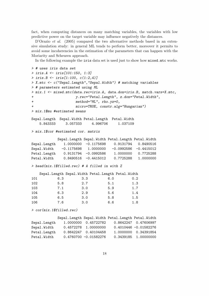
In the following example the iris data set is used just to show how mixed.mtc works.

> # uses iris data set

> iris.A <- iris[101:150, 1:3]

> iris.B <- iris[1:100, c(1:2,4)]

> X.mtc <- c("Sepal.Length","Sepal.Width") # matching variables

> # parameters estimated using ML

> mix.1 <- mixed.mtc(data.rec=iris.A, data.don=iris.B, match.vars=X.mtc,

+ y.rec="Petal.Length", z.don="Petal.Width",

+ method="ML", rho.yz=0,

+ micro=TRUE, constr.alg="Hungarian")

> mix.1$mu #estimated means

Sepal.Length Sepal.Width Petal.Length Petal.Width

5.843333 3.057333 4.996706 1.037109

> mix.1$cor #estimated cor. matrix


Sepal.Length 1.0000000 -0.1175698 0.9131794 0.8490516

Sepal.Width -0.1175698 1.0000000 -0.0992586 -0.4415012

Petal.Length 0.9131794 -0.0992586 1.0000000 0.7725288

Petal.Width 0.8490516 -0.4415012 0.7725288 1.0000000

> head(mix.1$filled.rec) # A filled in with Z


101 6.3 3.3 6.0 0.2

102 5.8 2.7 5.1 1.3

103 7.1 3.0 5.9 1.7

104 6.3 2.9 5.6 1.4

105 6.5 3.0 5.8 1.5

106 7.6 3.0 6.6 1.8

> cor(mix.1$filled.rec)


Sepal.Length 1.0000000 0.45722782 0.8642247 0.47606997

Sepal.Width 0.4572278 1.00000000 0.4010446 -0.01582276

Petal.Length 0.8642247 0.40104458 1.0000000 0.34391854

Petal.Width 0.4760700 -0.01582276 0.3439185 1.00000000

18

When using mixed.mtc the synthetic data set is provided in output as the compo-nent filled.rec of the list returned by calling it with the argument micro=TRUE. Whenmicro=FALSE the function mixed.mtc returns just the estimates of the parameters (para-metric macro approach).

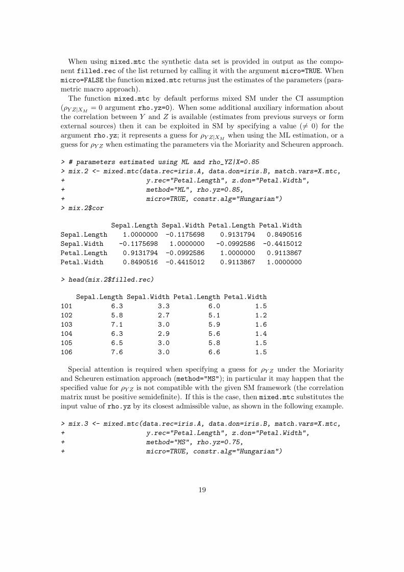
The function mixed.mtc by default performs mixed SM under the CI assumption(ρY Z|XM

= 0 argument rho.yz=0). When some additional auxiliary information aboutthe correlation between Y and Z is available (estimates from previous surveys or formexternal sources) then it can be exploited in SM by specifying a value (6= 0) for theargument rho.yz; it represents a guess for ρY Z|XM

when using the ML estimation, or aguess for ρY Z when estimating the parameters via the Moriarity and Scheuren approach.

> # parameters estimated using ML and rho_YZ|X=0.85



+ method="ML", rho.yz=0.85,


> mix.2$cor


Sepal.Length 1.0000000 -0.1175698 0.9131794 0.8490516

Sepal.Width -0.1175698 1.0000000 -0.0992586 -0.4415012

Petal.Length 0.9131794 -0.0992586 1.0000000 0.9113867

Petal.Width 0.8490516 -0.4415012 0.9113867 1.0000000

> head(mix.2$filled.rec)


101 6.3 3.3 6.0 1.5

102 5.8 2.7 5.1 1.2

103 7.1 3.0 5.9 1.6

104 6.3 2.9 5.6 1.4

105 6.5 3.0 5.8 1.5

106 7.6 3.0 6.6 1.5

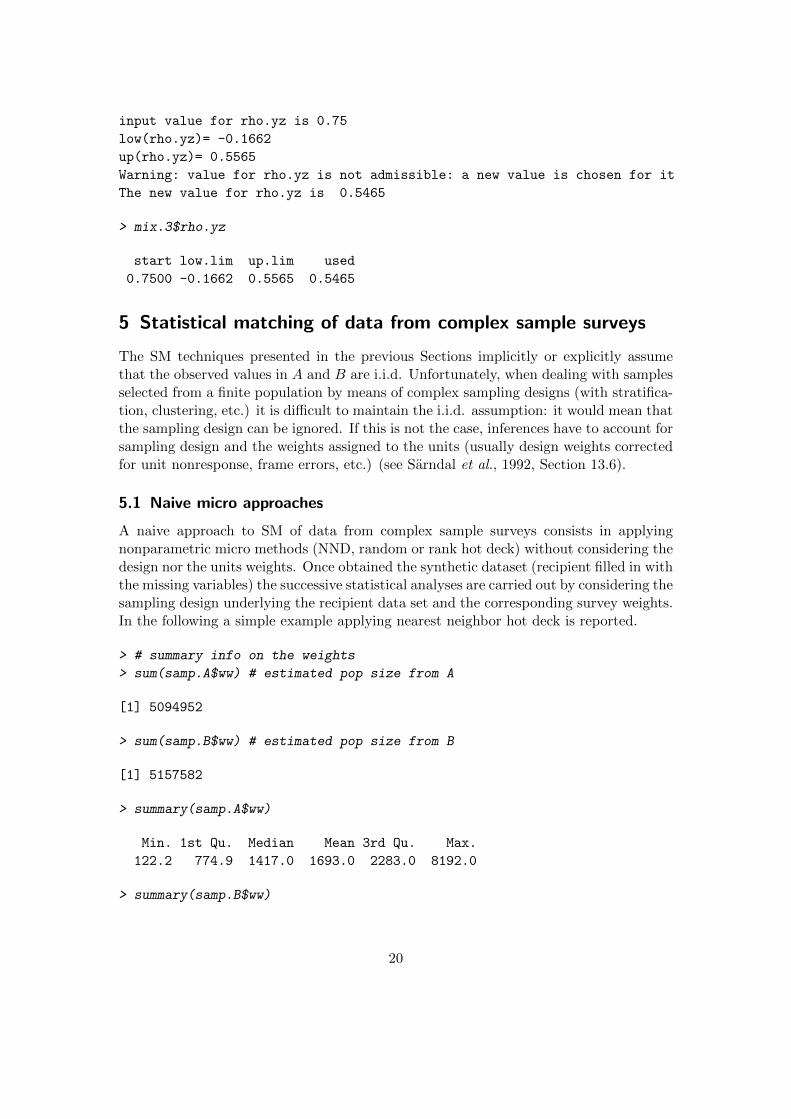
Special attention is required when specifying a guess for ρY Z under the Moriarityand Scheuren estimation approach (method="MS"); in particular it may happen that thespecified value for ρY Z is not compatible with the given SM framework (the correlationmatrix must be positive semidefinite). If this is the case, then mixed.mtc substitutes theinput value of rho.yz by its closest admissible value, as shown in the following example.



+ method="MS", rho.yz=0.75,


19

input value for rho.yz is 0.75

low(rho.yz)= -0.1662

up(rho.yz)= 0.5565

Warning: value for rho.yz is not admissible: a new value is chosen for it

The new value for rho.yz is 0.5465

> mix.3$rho.yz

start low.lim up.lim used

0.7500 -0.1662 0.5565 0.5465

5 Statistical matching of data from complex sample surveys

The SM techniques presented in the previous Sections implicitly or explicitly assumethat the observed values in A and B are i.i.d. Unfortunately, when dealing with samplesselected from a finite population by means of complex sampling designs (with stratifica-tion, clustering, etc.) it is difficult to maintain the i.i.d. assumption: it would mean thatthe sampling design can be ignored. If this is not the case, inferences have to account forsampling design and the weights assigned to the units (usually design weights correctedfor unit nonresponse, frame errors, etc.) (see Sarndal et al., 1992, Section 13.6).

5.1 Naive micro approaches

A naive approach to SM of data from complex sample surveys consists in applyingnonparametric micro methods (NND, random or rank hot deck) without considering thedesign nor the units weights. Once obtained the synthetic dataset (recipient filled in withthe missing variables) the successive statistical analyses are carried out by considering thesampling design underlying the recipient data set and the corresponding survey weights.In the following a simple example applying nearest neighbor hot deck is reported.

> # summary info on the weights

> sum(samp.A$ww) # estimated pop size from A

[1] 5094952

> sum(samp.B$ww) # estimated pop size from B

[1] 5157582

> summary(samp.A$ww)


122.2 774.9 1417.0 1693.0 2283.0 8192.0

> summary(samp.B$ww)

20


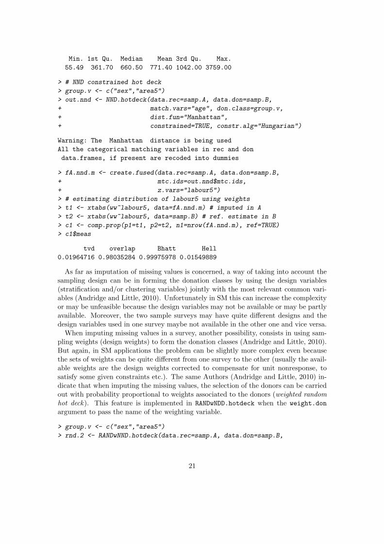
55.49 361.70 660.50 771.40 1042.00 3759.00

> # NND constrained hot deck


> out.nnd <- NND.hotdeck(data.rec=samp.A, data.don=samp.B,

+ match.vars="age", don.class=group.v,

+ dist.fun="Manhattan",

+ constrained=TRUE, constr.alg="Hungarian")




> fA.nnd.m <- create.fused(data.rec=samp.A, data.don=samp.B,

+ mtc.ids=out.nnd$mtc.ids,

+ z.vars="labour5")

> # estimating distribution of labour5 using weights

> t1 <- xtabs(ww~labour5, data=fA.nnd.m) # imputed in A

> t2 <- xtabs(ww~labour5, data=samp.B) # ref. estimate in B

> c1 <- comp.prop(p1=t1, p2=t2, n1=nrow(fA.nnd.m), ref=TRUE)

> c1$meas


0.01964716 0.98035284 0.99975978 0.01549889

As far as imputation of missing values is concerned, a way of taking into account thesampling design can be in forming the donation classes by using the design variables(stratification and/or clustering variables) jointly with the most relevant common vari-ables (Andridge and Little, 2010). Unfortunately in SM this can increase the complexityor may be unfeasible because the design variables may not be available or may be partlyavailable. Moreover, the two sample surveys may have quite different designs and thedesign variables used in one survey maybe not available in the other one and vice versa.

When imputing missing values in a survey, another possibility, consists in using sam-pling weights (design weights) to form the donation classes (Andridge and Little, 2010).But again, in SM applications the problem can be slightly more complex even becausethe sets of weights can be quite different from one survey to the other (usually the avail-able weights are the design weights corrected to compensate for unit nonresponse, tosatisfy some given constraints etc.). The same Authors (Andridge and Little, 2010) in-dicate that when imputing the missing values, the selection of the donors can be carriedout with probability proportional to weights associated to the donors (weighted randomhot deck). This feature is implemented in RANDwNDD.hotdeck when the weight.don

argument to pass the name of the weighting variable.



21

+ match.vars=NULL, don.class=group.v,

+ weight.don="ww")

> fA.wrnd <- create.fused(data.rec=samp.A, data.don=samp.B,


+ z.vars="labour5")

> # comparing marginal distribution of labour5 using weights

> tt.0w <- xtabs(ww~labour5, data=samp.B)

> tt.fw <- xtabs(ww~labour5, data=fA.wrnd)

> c1 <- comp.prop(p1=tt.fw, p2=tt.0w, n1=nrow(fA.wrnd), ref=TRUE)

> c1$meas


0.02129280 0.97870720 0.99972761 0.01650429

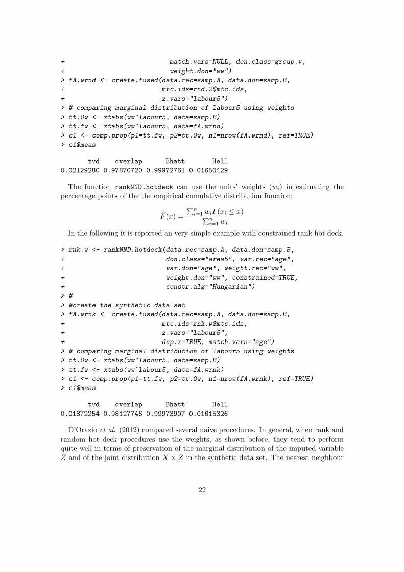
The function rankNND.hotdeck can use the units’ weights (wi) in estimating thepercentage points of the the empirical cumulative distribution function:

F (x) =

∑ni=1wiI (xi ≤ x)∑n

i=1wi

In the following it is reported an very simple example with constrained rank hot deck.

> rnk.w <- rankNND.hotdeck(data.rec=samp.A, data.don=samp.B,

+ don.class="area5", var.rec="age",

+ var.don="age", weight.rec="ww",

+ weight.don="ww", constrained=TRUE,

+ constr.alg="Hungarian")

> #

> #create the synthetic data set

> fA.wrnk <- create.fused(data.rec=samp.A, data.don=samp.B,

+ mtc.ids=rnk.w$mtc.ids,

+ z.vars="labour5",


> # comparing marginal distribution of labour5 using weights

> tt.0w <- xtabs(ww~labour5, data=samp.B)

> tt.fw <- xtabs(ww~labour5, data=fA.wrnk)

> c1 <- comp.prop(p1=tt.fw, p2=tt.0w, n1=nrow(fA.wrnk), ref=TRUE)

> c1$meas


0.01872254 0.98127746 0.99973907 0.01615326

D’Orazio et al. (2012) compared several naive procedures. In general, when rank andrandom hot deck procedures use the weights, as shown before, they tend to performquite well in terms of preservation of the marginal distribution of the imputed variableZ and of the joint distribution X × Z in the synthetic data set. The nearest neighbour

22

donor, performs well only when constrained matching is used and a design variable (usedin stratification) is considered in forming donation classes.

5.2 Statistical matching method that account explicitly for the samplingweights

In literature there are few SM methods that explicitly take into account the samplingdesign and the corresponding sampling weights: Renssen’s approach based on weights’calibrations (Renssen, 1998); Rubin’s file concatenation (Rubin, 1986) and the approachbased on the empirical likelihood proposed by Wu (2004). A comparison among theseapproaches can be found in D’Orazio et al. (2010).

The package StatMatch provides functions to apply the procedures suggested byRenssen (1998). Renssen’s approach consists in a series of calibration steps of the surveyweights in A and B in order to achieve consistency between estimates (mainly totals)computed separately from the two data sources. Calibration is a technique very commonin sample surveys for deriving new weights, as close as possible to the starting ones,which fulfill a series of constraints concerning totals for a set of auxiliary variables (forfurther details on calibration see Sarndal, 2005). The Renssen’s approach works wellwhen dealing with categorical variables or in a mixed case in which the number ofcontinuous variables is very limited. In the following it will be assumed that all thevariables (XD, Y, Z) are categorical, being XD a complete or an incomplete crossing ofthe matching variables XM . The procedure and the functions developed in StatMatchpermits to have one or more continuous variables (better just one) in the subset of thematching variables XM , while Y and Z can be both categorical or a combination ofthem is allowed (Y categorical and Z continuous, or vice versa).

The first step in the Renssen’s procedure consists in calibrating weights in A and in Bsuch that the new weights when applied to the set of the XD variables allow to reproducesome known (or estimated) population totals. In StatMatch the harmonization stepcan be performed by using harmonize.x. This function performs weights calibration (orpost-stratification) by means of functions available in the R package survey (Lumley,2004 and 2014). When the population totals are already known then they have to bepassed to harmonize.x via the argument x.tot; on the contrary, when they are unknown(x.tot=NULL) they are estimated by a weighted average of the totals estimated on thetwo surveys before the harmonization step:

tXD= λt

(A)XD

+ (1− λ) t(B)XD

being λ = nA/(nA + nB) (nA and nB are the sample sizes of A and B respectively)(Korn and Graubard, 1999, pp. 281–284).

The following example shows how to harmonize the joint distribution of the genderand classes of age with the data from the previous example, assuming that the jointdistribution of age and gender is not known in advance.

> tt.A <- xtabs(ww~sex+c.age, data=samp.A)

> tt.B <- xtabs(ww~sex+c.age, data=samp.B)

23

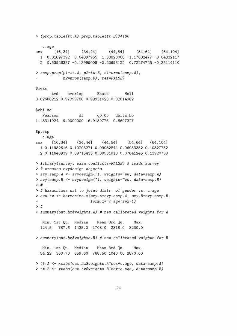
> (prop.table(tt.A)-prop.table(tt.B))*100

c.age

sex [16,34] (34,44] (44,54] (54,64] (64,104]

1 -0.01897392 -0.64897955 1.33820068 -1.17082477 -0.04332117

2 0.53926387 -0.13999008 -0.22698122 0.72274725 -0.35114110

> comp.prop(p1=tt.A, p2=tt.B, n1=nrow(samp.A),

+ n2=nrow(samp.B), ref=FALSE)

$meas


0.02600212 0.97399788 0.99931620 0.02614962

$chi.sq

Pearson df q0.05 delta.h0

11.3311924 9.0000000 16.9189776 0.6697327

$p.exp

c.age

sex [16,34] (34,44] (44,54] (54,64] (64,104]

1 0.11982616 0.10203271 0.09082844 0.06953352 0.10327752

2 0.11640939 0.09715433 0.08531810 0.07641245 0.13920738

> library(survey, warn.conflicts=FALSE) # loads survey

> # creates svydesign objects

> svy.samp.A <- svydesign(~1, weights=~ww, data=samp.A)

> svy.samp.B <- svydesign(~1, weights=~ww, data=samp.B)

> #

> # harmonizes wrt to joint distr. of gender vs. c.age

> out.hz <- harmonize.x(svy.A=svy.samp.A, svy.B=svy.samp.B,

+ form.x=~c.age:sex-1)

> #

> summary(out.hz$weights.A) # new calibrated weights for A


124.5 787.6 1435.0 1708.0 2318.0 8230.0

> summary(out.hz$weights.B) # new calibrated weights for B


54.22 360.70 659.60 768.50 1040.00 3870.00

> tt.A <- xtabs(out.hz$weights.A~sex+c.age, data=samp.A)

> tt.B <- xtabs(out.hz$weights.B~sex+c.age, data=samp.B)

24

> c1 <- comp.prop(p1=tt.A, p2=tt.B, n1=nrow(samp.A),


> c1$meas


8.326673e-17 1.000000e+00 1.000000e+00 0.000000e+00

The second step in the Renssen’s procedure consists in estimating the the joint dis-tribution Y and Z; in practice, when they both are categorical variables of two-waycontingency table Y × Z is the target of estimation; on the contrary, in the mixed case,the objective is the estimation of the total of the continuous variable for each categoryof the categorical one. When Y and Z are both categorical variables, in absence ofauxiliary information, the two-way contingency table Y × Z is estimated under the CIassumption by means of:

P(CIA)(Y=j,Z=k) = P

(A)Y=j|XD=i × P

(B)Z=k|XD=i × PXD=i

for i = 1, . . . , I; j = 1, . . . , J ; K = 1, . . . ,K;

In practice, P(A)Y=j|XD=i is computed from A; P

(B)Z=k|XD=i is computed from data in B

while PXD=i can be estimated indifferently from A or B (the data set are harmonizedwith respect to the XD distribution).

In StatMatch an estimate of the table Y × Z under the CIA is provided by thefunction comb.samples.

> # estimating c.netI vs. labour5 under the CI assumption

> out <- comb.samples(svy.A=out.hz$cal.A, svy.B=out.hz$cal.B,

+ svy.C=NULL, y.lab="c.neti", z.lab="labour5",

+ form.x=~c.age:sex-1)

> #

> addmargins(t(out$yz.CIA)) # table estimated under the CIA

(-Inf,0] (0,10] (10,15] (15,20] (20,25] (25,35]

1 371437.37 300036.37 274311.45 330113.82 211281.36 214834.05

2 66423.86 72968.22 72975.95 97978.40 62237.15 68317.71

3 77131.99 52710.28 46296.31 47966.68 28773.09 29169.28

4 71486.63 321060.02 252077.13 189783.80 88163.94 94066.02

5 396817.21 402085.73 270202.33 176110.31 110621.43 86631.14

Sum 983297.07 1148860.62 915863.16 841953.00 501076.98 493018.19

(35, Inf] Sum

1 105304.98 1807319.4

2 35320.81 476222.1

3 12929.49 294977.1

4 57905.82 1074543.4

5 42613.70 1485081.8

Sum 254074.80 5138143.8

25

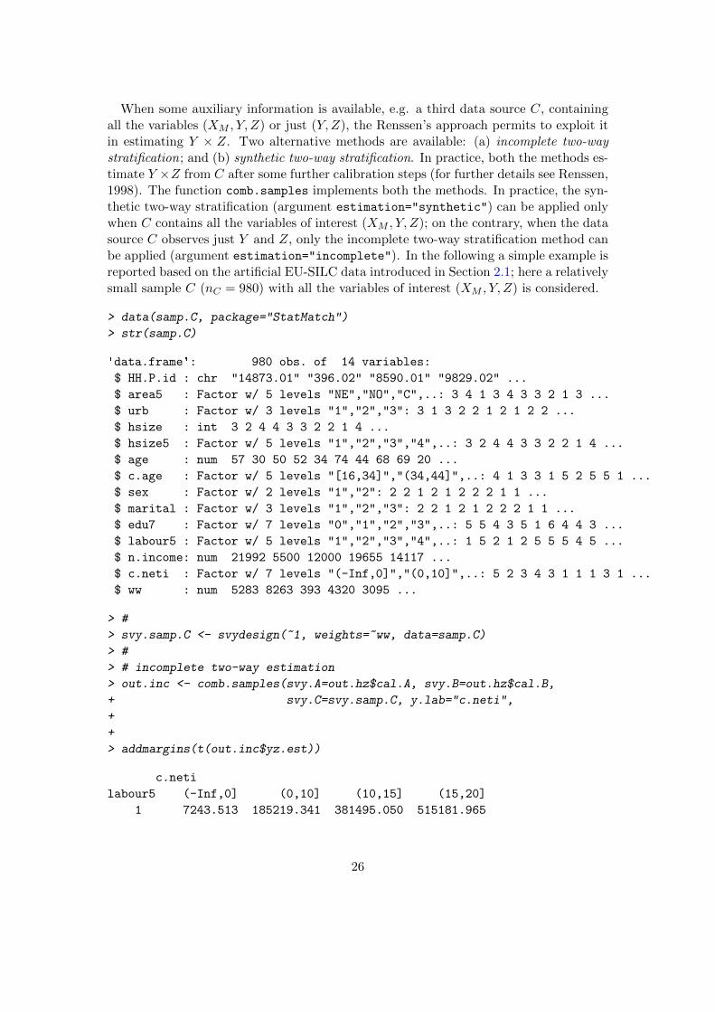
When some auxiliary information is available, e.g. a third data source C, containingall the variables (XM , Y, Z) or just (Y,Z), the Renssen’s approach permits to exploit itin estimating Y × Z. Two alternative methods are available: (a) incomplete two-waystratification; and (b) synthetic two-way stratification. In practice, both the methods es-timate Y ×Z from C after some further calibration steps (for further details see Renssen,1998). The function comb.samples implements both the methods. In practice, the syn-thetic two-way stratification (argument estimation="synthetic") can be applied onlywhen C contains all the variables of interest (XM , Y, Z); on the contrary, when the datasource C observes just Y and Z, only the incomplete two-way stratification method canbe applied (argument estimation="incomplete"). In the following a simple example isreported based on the artificial EU-SILC data introduced in Section 2.1; here a relativelysmall sample C (nC = 980) with all the variables of interest (XM , Y, Z) is considered.

> data(samp.C, package="StatMatch")

> str(samp.C)


$ HH.P.id : chr "14873.01" "396.02" "8590.01" "9829.02" ...



$ hsize : int 3 2 4 4 3 3 2 2 1 4 ...


$ age : num 57 30 50 52 34 74 44 68 69 20 ...



$ marital : Factor w/ 3 levels "1","2","3": 2 2 1 2 1 2 2 2 1 1 ...


$ labour5 : Factor w/ 5 levels "1","2","3","4",..: 1 5 2 1 2 5 5 5 4 5 ...

$ n.income: num 21992 5500 12000 19655 14117 ...

$ c.neti : Factor w/ 7 levels "(-Inf,0]","(0,10]",..: 5 2 3 4 3 1 1 1 3 1 ...

$ ww : num 5283 8263 393 4320 3095 ...

> #

> svy.samp.C <- svydesign(~1, weights=~ww, data=samp.C)

> #

> # incomplete two-way estimation

> out.inc <- comb.samples(svy.A=out.hz$cal.A, svy.B=out.hz$cal.B,

+ svy.C=svy.samp.C, y.lab="c.neti",

+ z.lab="labour5", form.x=~c.age:sex-1,

+ estimation="incomplete")

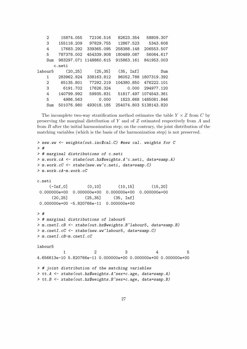
> addmargins(t(out.inc$yz.est))

c.neti

labour5 (-Inf,0] (0,10] (10,15] (15,20]

1 7243.513 185219.341 381495.050 515181.965

26

2 15874.055 72106.516 82623.354 58809.307

3 155118.209 97829.755 12867.523 5343.608

4 17683.292 339365.095 258388.148 206553.507

5 787378.002 454339.908 180489.087 56064.617

Sum 983297.071 1148860.615 915863.161 841953.003

c.neti

labour5 (20,25] (25,35] (35, Inf] Sum

1 283962.924 338163.812 96052.788 1807319.392

2 65135.801 77292.219 104380.850 476222.101

3 6191.702 17626.324 0.000 294977.120

4 140799.992 59935.831 51817.497 1074543.361

5 4986.563 0.000 1823.668 1485081.846

Sum 501076.980 493018.185 254074.803 5138143.820

The incomplete two-way stratification method estimates the table Y × Z from C bypreserving the marginal distribution of Y and of Z estimated respectively from A andfrom B after the initial harmonization step; on the contrary, the joint distribution of thematching variables (which is the basis of the harmonization step) is not preserved.

> new.ww <- weights(out.inc$cal.C) #new cal. weights for C

> #

> # marginal distributions of c.neti

> m.work.cA <- xtabs(out.hz$weights.A~c.neti, data=samp.A)

> m.work.cC <- xtabs(new.ww~c.neti, data=samp.C)

> m.work.cA-m.work.cC

c.neti

(-Inf,0] (0,10] (10,15] (15,20]

0.000000e+00 0.000000e+00 0.000000e+00 0.000000e+00

(20,25] (25,35] (35, Inf]

0.000000e+00 -5.820766e-11 0.000000e+00

> #

> # marginal distributions of labour5

> m.cnetI.cB <- xtabs(out.hz$weights.B~labour5, data=samp.B)

> m.cnetI.cC <- xtabs(new.ww~labour5, data=samp.C)

> m.cnetI.cB-m.cnetI.cC

labour5

1 2 3 4 5

4.656613e-10 5.820766e-11 0.000000e+00 0.000000e+00 0.000000e+00

> # joint distribution of the matching variables

> tt.A <- xtabs(out.hz$weights.A~sex+c.age, data=samp.A)

> tt.B <- xtabs(out.hz$weights.B~sex+c.age, data=samp.B)

27

> tt.C <- xtabs(new.ww~sex+c.age, data=samp.C)

> c1 <- comp.prop(p1=tt.A, p2=tt.B, n1=nrow(samp.A),


> c2 <- comp.prop(p1=tt.C, p2=tt.A, n1=nrow(samp.C),

+ n2=nrow(samp.A), ref=FALSE)

> c1$meas


8.326673e-17 1.000000e+00 1.000000e+00 0.000000e+00

> c2$meas


0.07017944 0.92982056 0.99689740 0.05570102

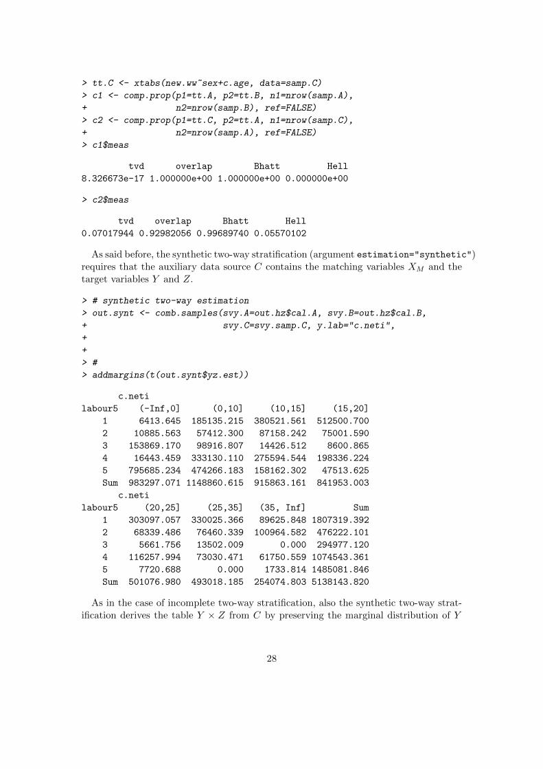
As said before, the synthetic two-way stratification (argument estimation="synthetic")requires that the auxiliary data source C contains the matching variables XM and thetarget variables Y and Z.

> # synthetic two-way estimation

> out.synt <- comb.samples(svy.A=out.hz$cal.A, svy.B=out.hz$cal.B,

+ svy.C=svy.samp.C, y.lab="c.neti",

+ z.lab="labour5", form.x=~c.age:sex-1,

+ estimation="synthetic")

> #

> addmargins(t(out.synt$yz.est))

c.neti

labour5 (-Inf,0] (0,10] (10,15] (15,20]

1 6413.645 185135.215 380521.561 512500.700

2 10885.563 57412.300 87158.242 75001.590

3 153869.170 98916.807 14426.512 8600.865

4 16443.459 333130.110 275594.544 198336.224

5 795685.234 474266.183 158162.302 47513.625

Sum 983297.071 1148860.615 915863.161 841953.003

c.neti

labour5 (20,25] (25,35] (35, Inf] Sum

1 303097.057 330025.366 89625.848 1807319.392

2 68339.486 76460.339 100964.582 476222.101

3 5661.756 13502.009 0.000 294977.120

4 116257.994 73030.471 61750.559 1074543.361

5 7720.688 0.000 1733.814 1485081.846

Sum 501076.980 493018.185 254074.803 5138143.820

As in the case of incomplete two-way stratification, also the synthetic two-way strat-ification derives the table Y × Z from C by preserving the marginal distribution of Y

28

and of Z estimated respectively from A and from B after the initial harmonization step;on the contrary, the joint distribution of the matching variables (which is the basis ofthe harmonization step) is still not preserved.

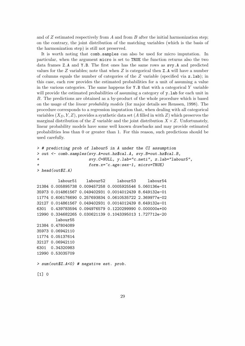
It is worth noting that comb.samples can also be used for micro imputation. Inparticular, when the argument micro is set to TRUE the function returns also the twodata frames Z.A and Y.B. The first ones has the same rows as svy.A and predictedvalues for the Z variables; note that when Z is categorical then Z.A will have a numberof columns equals the number of categories of the Z variable (specified via z.lab); inthis case, each row provides the estimated probabilities for a unit of assuming a valuein the various categories. The same happens for Y.B that with a categorical Y variablewill provide the estimated probabilities of assuming a category of y.lab for each unit inB. The predictions are obtained as a by-product of the whole procedure which is basedon the usage of the linear probability models (for major details see Renssen, 1998). Theprocedure corresponds to a regression imputation that, when dealing with all categoricalvariables (XD, Y, Z), provides a synthetic data set (A filled in with Z) which preserves themarginal distribution of the Z variable and the joint distribution X×Z. Unfortunately,linear probability models have some well known drawbacks and may provide estimatedprobabilities less than 0 or greater than 1. For this reason, such predictions should beused carefully.

> # predicting prob of labour5 in A under the CI assumption

> out <- comb.samples(svy.A=out.hz$cal.A, svy.B=out.hz$cal.B,

+ svy.C=NULL, y.lab="c.neti", z.lab="labour5",

+ form.x=~c.age:sex-1, micro=TRUE)

> head(out$Z.A)

labour51 labour52 labour53 labour54

21384 0.005895738 0.009457258 0.0005925546 5.060136e-01

35973 0.014861567 0.049402931 0.0014012439 8.649132e-01

11774 0.606176690 0.257693834 0.0610535722 2.369977e-02

32127 0.014861567 0.049402931 0.0014012439 8.649132e-01

6301 0.439783594 0.094976579 0.1220299990 0.000000e+00

12990 0.334682265 0.030621139 0.1043395013 1.727712e-20

labour55

21384 0.47804089

35973 0.06942110

11774 0.05137614

32127 0.06942110

6301 0.34320983

12990 0.53035709

> sum(out$Z.A<0) # negative est. prob.

[1] 0

29

> sum(out$Z.A>1) # est. prob. >1

[1] 0

> # compare marginal distributions of Z

> t.zA <- colSums(out$Z.A * out.hz$weights.A)

> t.zB <- xtabs(out.hz$weights.B ~ samp.B$labour5)

> c1 <- comp.prop(p1=t.zA, p2=t.zB, n1=nrow(samp.A), ref=TRUE)

> c1$meas


2.185752e-16 1.000000e+00 1.000000e+00 1.053671e-08

D’orazio et al. (2012) suggest using a randomization mechanism to derive the predictedcategory starting from the estimated probabilities.

> # predicting categories of labour5 in A

> # randomized prediction with prob proportional to estimated prob.

> pps1 <- function(x) sample(x=1:length(x), size=1, prob=x)

> pred.zA <- apply(out$Z.A, 1, pps1)

> samp.A$labour5 <- factor(pred.zA, levels=1:nlevels(samp.B$labour5),

+ labels=as.character(levels(samp.B$labour5)),

+ ordered=T)

> # comparing marginal distributions of Z

> t.zA <- xtabs(out.hz$weights.A ~ samp.A$labour5)

> c1 <- comp.prop(p1=t.zA, p2=t.zB, n1=nrow(samp.A), ref=TRUE)

> c1$meas


0.01281817 0.98718183 0.99985951 0.01185287

> # comparing joint distributions of X vs. Z

> t.xzA <- xtabs(out.hz$weights.A~c.age+sex+labour5, data=samp.A)

> t.xzB <- xtabs(out.hz$weights.B~c.age+sex+labour5, data=samp.B)

> out.comp <- comp.prop(p1=t.xzA, p2=t.xzB, n1=nrow(samp.A), ref=TRUE)

> out.comp$meas


0.04682085 0.95317915 0.99739102 0.05107817

> out.comp$chi.sq


66.305895 46.000000 62.829620 1.055329

30

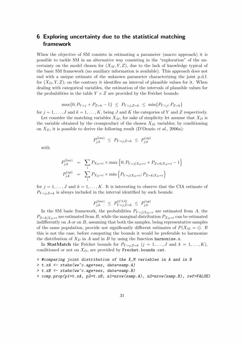
6 Exploring uncertainty due to the statistical matchingframework

When the objective of SM consists in estimating a parameter (macro approach) it ispossible to tackle SM in an alternative way consisting in the “exploration” of the un-certainty on the model chosen for (XM , Y, Z), due to the lack of knowledge typical ofthe basic SM framework (no auxiliary information is available). This approach does notend with a unique estimate of the unknown parameter characterizing the joint p.d.f.for (XD, Y, Z); on the contrary it identifies an interval of plausible values for it. Whendealing with categorical variables, the estimation of the intervals of plausible values forthe probabilities in the table Y × Z are provided by the Frechet bounds:

max{0;PY=j + PZ=k − 1} ≤ PY=j,Z=k ≤ min{PY=j ;PZ=k}

for j = 1, . . . , J and k = 1, . . . ,K, being J and K the categories of Y and Z respectively.Let consider the matching variables XM , for sake of simplicity let assume that XD is

the variable obtained by the crossproduct of the chosen XM variables; by conditioningon XD, it is possible to derive the following result (D’Orazio et al., 2006a):

P(low)j,k ≤ PY=j,Z=k ≤ P

(up)j,k

with

P(low)j,k =

∑i

PXD=i ×max{

0;PY=j|XD=i + PZ=k|XD=i − 1}

P(up)j,k =

∑i

PXD=i ×min{PY=j|XD=i;PZ=k|XD=i

}for j = 1, . . . , J and k = 1, . . . ,K. It is interesting to observe that the CIA estimate ofPY=j,Z=k is always included in the interval identified by such bounds:

P(low)j,k ≤ P

(CIA)Y=j,Z=k ≤ P

(up)j,k

In the SM basic framework, the probabilities PY=j|XD=i are estimated from A, thePZ=k|XD=i are estimated fromB, while the marginal distribution PXD=i can be estimatedindifferently on A or on B, assuming that both the samples, being representative samplesof the same population, provide not significantly different estimates of P (XM = i). Ifthis is not the case, before computing the bounds it would be preferable to harmonizethe distribution of XD in A and in B by using the function harmonize.x.

In StatMatch the Frechet bounds for PY=j,Z=k (j = 1, . . . , J and k = 1, . . . ,K),conditioned or not on XD, are provided by Frechet.bounds.cat.

> #comparing joint distribution of the X_M variables in A and in B

> t.xA <- xtabs(ww~c.age+sex, data=samp.A)

> t.xB <- xtabs(ww~c.age+sex, data=samp.B)

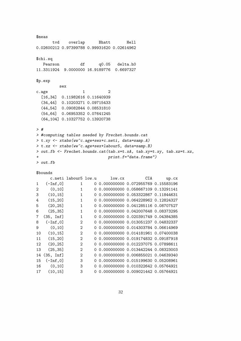
> comp.prop(p1=t.xA, p2=t.xB, n1=nrow(samp.A), n2=nrow(samp.B), ref=FALSE)

31

$meas


0.02600212 0.97399788 0.99931620 0.02614962

$chi.sq


11.3311924 9.0000000 16.9189776 0.6697327

$p.exp

sex

c.age 1 2

[16,34] 0.11982616 0.11640939

(34,44] 0.10203271 0.09715433

(44,54] 0.09082844 0.08531810

(54,64] 0.06953352 0.07641245

(64,104] 0.10327752 0.13920738

> #

> #computing tables needed by Frechet.bounds.cat

> t.xy <- xtabs(ww~c.age+sex+c.neti, data=samp.A)

> t.xz <- xtabs(ww~c.age+sex+labour5, data=samp.B)

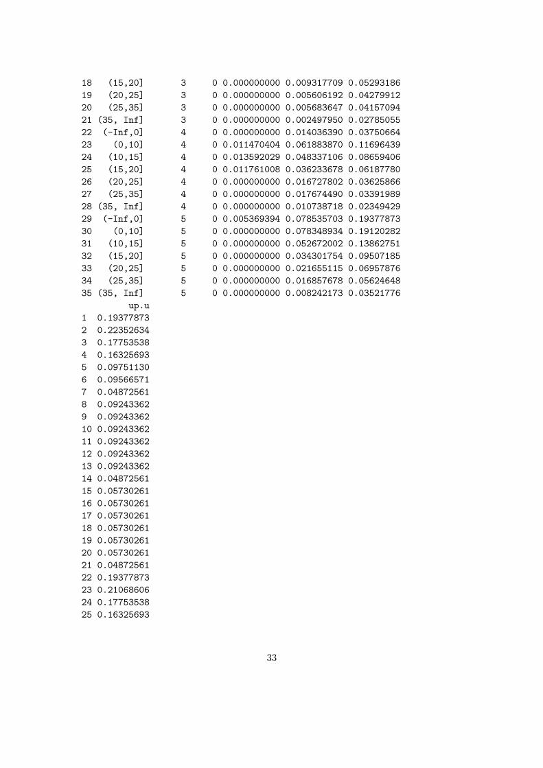
> out.fb <- Frechet.bounds.cat(tab.x=t.xA, tab.xy=t.xy, tab.xz=t.xz,

+ print.f="data.frame")

> out.fb

$bounds

c.neti labour5 low.u low.cx CIA up.cx

1 (-Inf,0] 1 0 0.000000000 0.072955769 0.15583196

2 (0,10] 1 0 0.000000000 0.058667109 0.13291141

3 (10,15] 1 0 0.000000000 0.053322867 0.11844631

4 (15,20] 1 0 0.000000000 0.064228962 0.12824327

5 (20,25] 1 0 0.000000000 0.041285116 0.08707527

6 (25,35] 1 0 0.000000000 0.042007648 0.08373295

7 (35, Inf] 1 0 0.000000000 0.020391749 0.04384385

8 (-Inf,0] 2 0 0.000000000 0.013051237 0.04832337

9 (0,10] 2 0 0.000000000 0.014303784 0.06614969

10 (10,15] 2 0 0.000000000 0.014181961 0.07400038

11 (15,20] 2 0 0.000000000 0.019174832 0.09187918

12 (20,25] 2 0 0.000000000 0.012237075 0.07898611

13 (25,35] 2 0 0.000000000 0.013442244 0.08323003

14 (35, Inf] 2 0 0.000000000 0.006855021 0.04639340

15 (-Inf,0] 3 0 0.000000000 0.015199630 0.05208961

16 (0,10] 3 0 0.000000000 0.010322642 0.05764921

17 (10,15] 3 0 0.000000000 0.009021442 0.05764921

32

18 (15,20] 3 0 0.000000000 0.009317709 0.05293186

19 (20,25] 3 0 0.000000000 0.005606192 0.04279912

20 (25,35] 3 0 0.000000000 0.005683647 0.04157094

21 (35, Inf] 3 0 0.000000000 0.002497950 0.02785055

22 (-Inf,0] 4 0 0.000000000 0.014036390 0.03750664

23 (0,10] 4 0 0.011470404 0.061883870 0.11696439

24 (10,15] 4 0 0.013592029 0.048337106 0.08659406

25 (15,20] 4 0 0.011761008 0.036233678 0.06187780

26 (20,25] 4 0 0.000000000 0.016727802 0.03625866

27 (25,35] 4 0 0.000000000 0.017674490 0.03391989

28 (35, Inf] 4 0 0.000000000 0.010738718 0.02349429

29 (-Inf,0] 5 0 0.005369394 0.078535703 0.19377873

30 (0,10] 5 0 0.000000000 0.078348934 0.19120282

31 (10,15] 5 0 0.000000000 0.052672002 0.13862751

32 (15,20] 5 0 0.000000000 0.034301754 0.09507185

33 (20,25] 5 0 0.000000000 0.021655115 0.06957876

34 (25,35] 5 0 0.000000000 0.016857678 0.05624648

35 (35, Inf] 5 0 0.000000000 0.008242173 0.03521776

up.u

1 0.19377873

2 0.22352634

3 0.17753538

4 0.16325693

5 0.09751130

6 0.09566571

7 0.04872561

8 0.09243362

9 0.09243362

10 0.09243362

11 0.09243362

12 0.09243362

13 0.09243362

14 0.04872561

15 0.05730261

16 0.05730261

17 0.05730261

18 0.05730261

19 0.05730261

20 0.05730261

21 0.04872561

22 0.19377873

23 0.21068606

24 0.17753538

25 0.16325693

33

26 0.09751130

27 0.09566571

28 0.04872561

29 0.19377873

30 0.22352634

31 0.17753538

32 0.16325693

33 0.09751130

34 0.09566571

35 0.04872561

$uncertainty

av.u av.cx

0.1138008 0.0773067

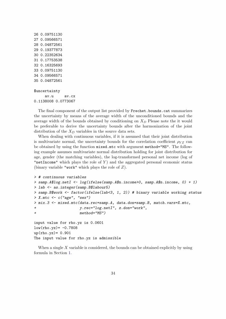
The final component of the output list provided by Frechet.bounds.cat summarizesthe uncertainty by means of the average width of the unconditioned bounds and theaverage width of the bounds obtained by conditioning on XD Please note the it wouldbe preferable to derive the uncertainty bounds after the harmonization of the jointdistribution of the XD variables in the source data sets.

When dealing with continuous variables, if it is assumed that their joint distributionis multivariate normal, the uncertainty bounds for the correlation coefficient ρY Z canbe obtained by using the function mixed.mtc with argument method="MS". The follow-ing example assumes multivariate normal distribution holding for joint distribution forage, gender (the matching variables), the log-transformed personal net income (log of"netIncome" which plays the role of Y ) and the aggregated personal economic status(binary variable "work" which plays the role of Z).

> # continuous variables

> samp.A$log.netI <- log(ifelse(samp.A$n.income>0, samp.A$n.income, 0) + 1)

> lab <- as.integer(samp.B$labour5)

> samp.B$work <- factor(ifelse(lab<3, 1, 2)) # binary variable working status

> X.mtc <- c("age", "sex")

> mix.3 <- mixed.mtc(data.rec=samp.A, data.don=samp.B, match.vars=X.mtc,

+ y.rec="log.netI", z.don="work",

+ method="MS")

input value for rho.yz is 0.0601

low(rho.yz)= -0.7808

up(rho.yz)= 0.901

The input value for rho.yz is admissible

When a single X variable is considered, the bounds can be obtained explicitly by usingformula in Section 1.

34

References

Andridge R.R., Little R.J.A. (2009) “The Use of Sample Weights in Hot Deck Imputation”.Journal of Official Statistics, 25(1), 21–36.

Andridge R.R., Little R.J.A. (2010) “A Review of Hot Deck Imputation for SurveyNonresponse”. International Statistical Review, 78, 40–64.

Berkelaar M. and others (2015) “lpSolve: Interface to Lpsolve v. 5.5 to solve linear–integerprograms”. R package version 5.6.13. http://CRAN.R-project.org/package=lpSolve

Breiman, L. (2001) “Random Forests”, Machine Learning, 45(1), 5–32.

Breiman L., Friedman J. H., Olshen R. A., and Stone, C. J. (1984) Classification andRegression Trees. Wadsworth.

Cohen M.L. (1991) “Statistical matching and microsimulation models”, in Citro andHanushek (eds) Improving Information for Social Policy Decisions: The Uses ofMicrosimulation Modeling. Vol II Technical papers. Washington D.C.

D’Orazio M. (2010) “Statistical matching when dealing with data from complex surveysampling”, in Report of WP1. State of the art on statistical methodologies for dataintegration, ESSnet project on Data Integration, 33–37,http://www.essnet-portal.eu/sites/default/files/131/ESSnetDI_WP1_v1.32.pdf

D’Orazio M. (2016) “StatMatch: Statistical Matching”. R package version 1.2.5.http://CRAN.R-project.org/package=StatMatch

D’Orazio M., Di Zio M., Scanu, M. (2005) “A comparison among different estimators ofregression parameters on statistically matched files trough an extensive simulationstudy”. Contributi Istat, 2005/10

D’Orazio M., Di Zio M., Scanu M. (2006a) “Statistical matching for categorical data:Displaying uncertainty and using logical constraints”. Journal of Official Statistics 22,137–157.

D’Orazio M., Di Zio M., Scanu M. (2006b) Statistical matching: Theory and practice. Wiley,Chichester.

D’Orazio M., Di Zio M., Scanu M. (2008) “The statistical matching workflow”, in: Report ofWP1: State of the art on statistical methodologies for integration of surveys andadministrative data, “ESSnet Statistical Methodology Project on Integration of Surveyand Administrative Data”, 25–26. http://cenex-isad.istat.it/

D’Orazio M., Di Zio M., Scanu M. (2010) “Old and new approaches in statistical matchingwhen samples are drawn with complex survey designs”. Proceedings of the 45th“Riunione Scientifica della Societa’ Italiana di Statistica”, Padova 16–18 June 2010.

D’Orazio M., Di Zio M., Scanu M. (2012) “Statistical Matching of Data from ComplexSample Surveys”. Proceedings of the European Conference on Quality in OfficialStatistics - Q2012, 29 May–1 June 2012, Athens, Greece.

Gower J. C. (1971) “A general coefficient of similarity and some of its properties”.Biometrics, 27, 623–637.

Harrell F.E. (2001) Regression Modeling Strategies With Applications to Linear Models,Logistic Regression, and Survival Analysis. New York, Springer

Harrell F.E., with contributions from Charles Dupont and many others (2016). “Hmisc:Harrell Miscellaneous”. R package version 4.0-1.https://CRAN.R-project.org/package=Hmisc

35

http://CRAN.R-project.org/package=lpSolve

http://www.essnet-portal.eu/sites/default/files/131/ESSnetDI_WP1_v1.32.pdf

http://CRAN.R-project.org/package=StatMatch

http://cenex-isad.istat.it/

https://CRAN.R-project.org/package=Hmisc

Hornik K. (2005). “A CLUE for CLUster Ensembles”. Journal of Statistical Software 14/12.http://www.jstatsoft.org/v14/i12/.

Hornik K. (2014). “clue: Cluster ensembles”. R package version 0.3-48.http://CRAN.R-project.org/package=clue.

Korn E.L., Graubard B.I. (1999) Analysis of Health Surveys. Wiley, New York

Kovar J.G., MacMillan J., Whitridge P. (1988) “Overview and strategy for the GeneralizedEdit and Imputation System”. Statistics Canada, Methodology Working Paper, No.BSMD 88-007 E/F.

Liaw A., Wiener M. (2002) “Classification and Regression by randomForest”. R News, 2(3),18–22.

Lumley T. (2004) “Analysis of complex survey samples”. Journal of Statistical Software, 9(1):1-19

Lumley T. (2016) “survey: analysis of complex survey samples”. R package version 3.31-5.http://CRAN.R-project.org/package=survey

Meyer D., Buchta C. (2016) “proxy: Distance and Similarity Measures”. R package version0.4-16. http://CRAN.R-project.org/package=proxy

Moriarity C., Scheuren F. (2001) “Statistical matching: a paradigm for assessing theuncertainty in the procedure”. Journal of Official Statistics, 17, 407–422.

Moriarity C., Scheuren F. (2003). “A note on Rubin’s statistical matching using fileconcatenation with adjusted weights and multiple imputation”, Jour. of Business andEconomic Statistics, 21, 65–73.

R Core Team (2016) R: A language and environment for statistical computing. R Foundationfor Statistical Computing, Vienna, Austria. http://www.R-project.org/.

Rassler S. (2002) Statistical matching: a frequentist theory, practical applications andalternative Bayesian approaches. Springer Verlag, New York.

Renssen R.H.(1998) “Use of statistical matching techniques in calibration estimation”. SurveyMethodology 24, 171–183.

Rubin D.B. (1986) “Statistical matching using file concatenation with adjusted weights andmultiple imputations”. Journal of Business and Economic Statistics, 4, 87–94.

Sarndal C.E., Swensson B., Wretman J. (1992) Model Assisted Survey Sampling.Springer-Verlag, New York.

Sarndal C.E., Lundstrom S. (2005) Estimation in Surveys with Nonresponse. Wiley, NewYork.

Scanu M. (2008) “The practical aspects to be considered for statistical matching”. in: Reportof WP2: Recommendations on the use of methodologies for the integration of surveys andadministrative data, “ESSnet Statistical Methodology Project on Integration of Surveyand Administrative Data”, 34–35. http://cenex-isad.istat.it/

Singh A.C., Mantel H., Kinack M., Rowe G. (1993) “Statistical matching: use of auxiliaryinformation as an alternative to the conditional independence assumption”. SurveyMethodology, 19, 59–79.

Wu C. (2004) “Combining information from multiple surveys through the empirical likelihoodmethod”. The Canadian Journal of Statistics, 32, 15–26.

36

http://www.jstatsoft.org/v14/i12/

http://CRAN.R-project.org/package=clue

http://CRAN.R-project.org/package=survey

http://CRAN.R-project.org/package=proxy

http://www.R-project.org/

http://cenex-isad.istat.it/

Statistical Matching and Imputation of Survey Data with ... · Statistical matching techniques aim...

Documents

Transcript of Statistical Matching and Imputation of Survey Data with ... · Statistical matching techniques aim...