1

Statistical Machine Translation

Bonnie Dorr Christof Monz

CMSC 723: Introduction to Computational Linguistics

Lecture 8

October 27, 2004

2

Overview

Why MT Statistical vs. rule-based MT Computing translation probabilities from a

parallel corpus IBM Models 1-3

3

A Brief History

Machine translation was one of the first applications envisioned for computers

Warren Weaver (1949): “I have a text in front of me which is written in Russian but I am going to pretend that it is really written in English and that it has been coded in some strange symbols. All I need to do is strip off the code in order to retrieve the information contained in the text.”

First demonstrated by IBM in 1954 with a basic word-for-word translation system

4

Interest in MT

Commercial interest:U.S. has invested in MT for intelligence

purposesMT is popular on the web—it is the most used

of Google’s special featuresEU spends more than $1 billion on translation

costs each year.(Semi-)automated translation could lead to

huge savings

5

Interest in MT

Academic interest: One of the most challenging problems in NLP

research Requires knowledge from many NLP sub-areas, e.g.,

lexical semantics, parsing, morphological analysis, statistical modeling,…

Being able to establish links between two languages allows for transferring resources from one language to another

6

Rule-Based vs. Statistical MT

Rule-based MT: Hand-written transfer rules Rules can be based on lexical or structural transfer Pro: firm grip on complex translation phenomena Con: Often very labor-intensive -> lack of robustness

Statistical MT Mainly word or phrase-based translations Translation are learned from actual data Pro: Translations are learned automatically Con: Difficult to model complex translation phenomena

7

Parallel Corpus

Example from DE-News (8/1/1996)English GermanDiverging opinions about planned tax reform

Unterschiedliche Meinungen zur geplanten Steuerreform

The discussion around the envisaged major tax reform continues .

Die Diskussion um die vorgesehene grosse Steuerreform dauert an .

The FDP economics expert , Graf Lambsdorff , today came out in favor of advancing the enactment of significant parts of the overhaul , currently planned for 1999 .

Der FDP - Wirtschaftsexperte Graf Lambsdorff sprach sich heute dafuer aus , wesentliche Teile der fuer 1999 geplanten Reform vorzuziehen .

8

Word-Level Alignments

Given a parallel sentence pair we can link (align) words or phrases that are translations of each other:

9

Parallel Resources

Newswire: DE-News (German-English), Hong-Kong News, Xinhua News (Chinese-English),

Government: Canadian-Hansards (French-English), Europarl (Danish, Dutch, English, Finnish, French, German, Greek, Italian, Portugese, Spanish, Swedish), UN Treaties (Russian, English, Arabic, . . . )

Manuals: PHP, KDE, OpenOffice (all from OPUS, many languages)

Web pages: STRAND project (Philip Resnik)

10

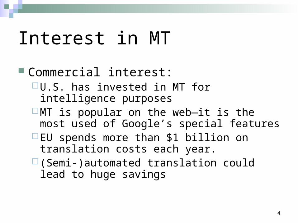
Sentence Alignment

If document De is translation of document Df how do we find the translation for each sentence?

The n-th sentence in De is not necessarily the translation of the n-th sentence in document Df

In addition to 1:1 alignments, there are also 1:0, 0:1, 1:n, and n:1 alignments

Approximately 90% of the sentence alignments are 1:1

11

Sentence Alignment (c’ntd)

There are several sentence alignment algorithms: Align (Gale & Church): Aligns sentences based on their

character length (shorter sentences tend to have shorter translations then longer sentences). Works astonishingly well

Char-align: (Church): Aligns based on shared character sequences. Works fine for similar languages or technical domains

K-Vec (Fung & Church): Induces a translation lexicon from the parallel texts based on the distribution of foreign-English word pairs.

12

Computing Translation Probabilities

Given a parallel corpus we can estimate P(e | f) The maximum likelihood estimation of P(e | f) is: freq(e,f)/freq(f)

Way too specific to get any reasonable frequencies! Vast majority of unseen data will have zero counts!

P(e | f ) could be re-defined as:

Problem: The English words maximizing P(e | f ) might not result in a readable sentence

P(e | f ) maxeif j

P(ei | f j )

13

Computing Translation Probabilities (c’tnd)

We can account for adequacy: each foreign word translates into its most likely English word

We cannot guarantee that this will result in a fluent English sentence

Solution: transform P(e | f) with Bayes’ rule: P(e | f) = P(e) P(f | e) / P(f)

P(f | e) accounts for adequacy P(e) accounts for fluency

14

Decoding

The decoder combines the evidence from P(e) and P(f | e) to find the sequence e that is the best translation:

The choice of word e’ as translation of f’ depends on the translation probability P(f’ | e’) and on the context, i.e. other English words preceding e’

argmaxe

P(e | f ) argmaxe

P( f | e)P(e)

15

Noisy Channel Model for Translation

16

Language Modeling

Determines the probability of some English sequence of length l

P(e) is hard to estimate directly, unless l is very small

P(e) is normally approximated as:

where m is size of the context, i.e. number of previous words that are considered, normally m=2 (tri-gram language model

e1l

P(e1l ) P(e1 ) P(eii2

l | e1i 1)

P(e1l ) P(e1 )P(e2 | e1) P(eii3

l | ei mi 1 )

17

Translation Modeling

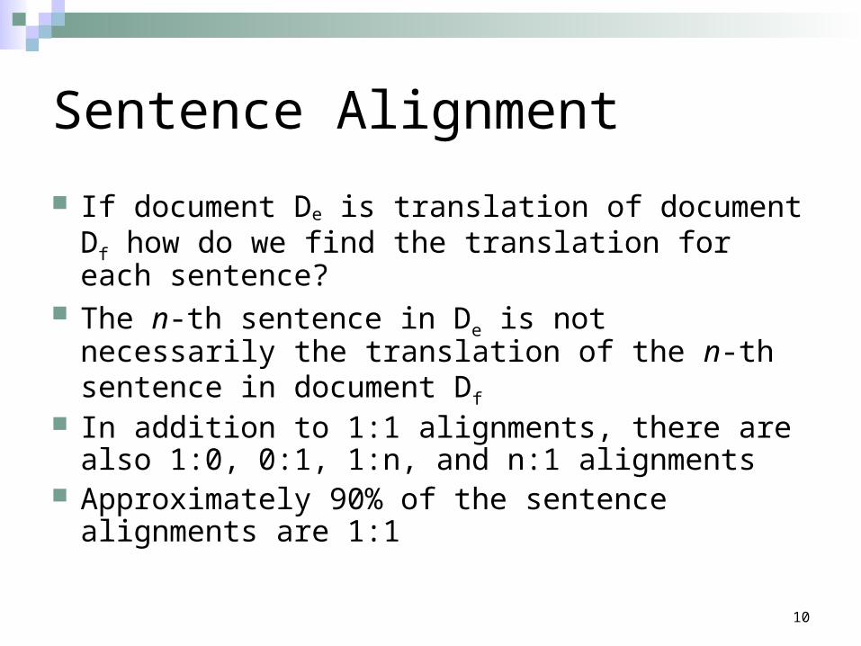
Determines the probability that the foreign word f is a translation of the English word e

How to compute P(f | e) from a parallel corpus? Statistical approaches rely on the co-occurrence

of e and f in the parallel data: If e and f tend to co-occur in parallel sentence pairs, they are likely to be translations of one another

18

Finding Translations in a Parallel Corpus

Into which foreign words f, . . . , f’ does e translate? Commonly, four factors are used:

How often do e and f co-occur? (translation) How likely is a word occurring at position i to translate into a

word occurring at position j? (distortion) For example: English is a verb-second language, whereas German is a verb-final language

How likely is e to translate into more than one word? (fertility) For example: defeated can translate into eine Niederlage erleiden

How likely is a foreign word to be spuriously generated? (null translation)

19

Translation Steps

20

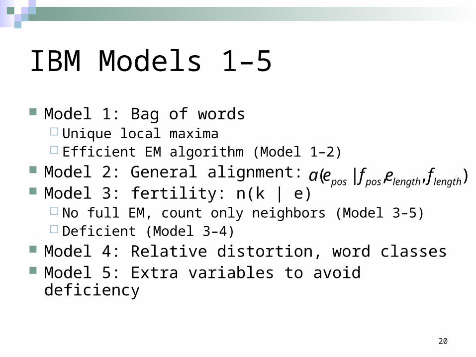
IBM Models 1–5

Model 1: Bag of words Unique local maxima Efficient EM algorithm (Model 1–2)

Model 2: General alignment: Model 3: fertility: n(k | e)

No full EM, count only neighbors (Model 3–5) Deficient (Model 3–4)

Model 4: Relative distortion, word classes Model 5: Extra variables to avoid deficiency

a(epos | f pos,elength, f length )

21

IBM Model 1 Given an English sentence e1 . . . el and a foreign sentence

f1 . . . fm We want to find the ’best’ alignment a, where a is a set pairs of

the form {(i , j), . . . , (i’, j’)}, 0<= i , i’ <= l and 1<= j , j’<= m Note that if (i , j), (i’, j) are in a, then i equals i’, i.e. no many-to-

one alignments are allowed Note we add a spurious NULL word to the English sentence at

position 0 In total there are (l + 1)m different alignments A Allowing for many-to-many alignments results in (2l)m possible

alignments A

22

IBM Model 1

Simplest of the IBM models Does not consider word order (bag-of-

words approach) Does not model one-to-many alignments Computationally inexpensive Useful for parameter estimations that are

passed on to more elaborate models

23

IBM Model 1

Translation probability in terms of alignments:

where:

and:

P( f | e) P( f ,a | e)aA

P( f ,a | e) P(a | e)P( f | a,e)

1

(l 1)mP( f j

j1

m

| ea j )

P( f | e) 1

(l 1)mP( f j

j1

m

| ea j )aA

24

IBM Model 1

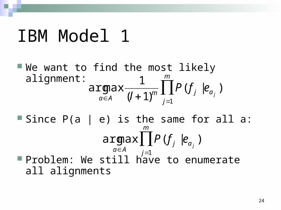
We want to find the most likely alignment:

Since P(a | e) is the same for all a:

Problem: We still have to enumerate all alignments

argmaxaA

1

(l 1)mP( f j

j1

m

| ea j )

argmaxaA

P( f jj1

m

| ea j )

25

IBM Model 1

Since P(fj | ei) is independent from P(fj’ | ei’) we can find the maximum alignment by looking at the individual translation probabilities only

Let , then for each aj:

The best alignment can computed in a quadratic number of steps: (l+1 x m)

argmaxaA

(a1, ... ,am )

a j argmax0il

P( f j | ei)

26

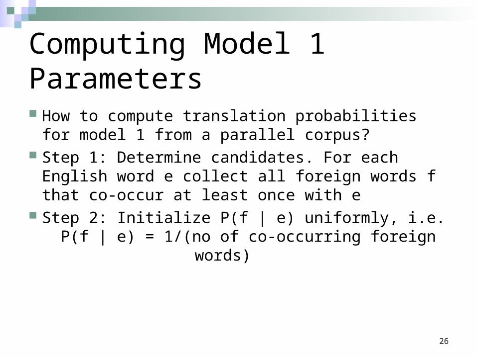
Computing Model 1 Parameters

How to compute translation probabilities for model 1 from a parallel corpus?

Step 1: Determine candidates. For each English word e collect all foreign words f that co-occur at least once with e

Step 2: Initialize P(f | e) uniformly, i.e. P(f | e) = 1/(no of co-occurring foreign

words)

27

Computing Model 1 Parameters

Step 3: Iteratively refine translation probablities:1 for n iterations

2 set tc to zero3 for each sentence pair (e,f) of lengths (l,m)4 for j=1 to m

5 total=0; 6 for i=1 to l

7 total += P(fj | ei); 8 for i=1 to l

9 tc(fj | ei) += P(fj | ei)/total; 10 for each word e 11 total=0; 12 for each word f s.t. tc(f | e) is defined 13 total += tc(f | e); 14 for each word f s.t. tc(f | e) is defined 15 P(f | e) = tc(f | e)/total;

28

IBM Model 1 Example

Parallel ‘corpus’:the dog :: le chienthe cat :: le chat

Step 1+2 (collect candidates and initialize uniformly):P(le | the) = P(chien | the) = P(chat | the) = 1/3P(le | dog) = P(chien | dog) = P(chat | dog) = 1/3P(le | cat) = P(chien | cat) = P(chat | cat) = 1/3P(le | NULL) = P(chien | NULL) = P(chat | NULL) = 1/3

29

IBM Model 1 Example

Step 3: Iterate NULL the dog :: le chien

j=1 total = P(le | NULL)+P(le | the)+P(le | dog)= 1tc(le | NULL) += P(le | NULL)/1 = 0 += .333/1 = 0.333tc(le | the) += P(le | the)/1 = 0 += .333/1 = 0.333tc(le | dog) += P(le | dog)/1 = 0 += .333/1 = 0.333

j=2total = P(chien | NULL)+P(chien | the)+P(chien | dog)=1tc(chien | NULL) += P(chien | NULL)/1 = 0 += .333/1 = 0.333tc(chien | the) += P(chien | the)/1 = 0 += .333/1 = 0.333tc(chien | dog) += P(chien | dog)/1 = 0 += .333/1 = 0.333

30

IBM Model 1 Example

NULL the cat :: le chat j=1

total = P(le | NULL)+P(le | the)+P(le | cat)=1tc(le | NULL) += P(le | NULL)/1 = 0.333 += .333/1 = 0.666tc(le | the) += P(le | the)/1 = 0.333 += .333/1 = 0.666tc(le | cat) += P(le | cat)/1 = 0 +=.333/1 = 0.333

j=2total = P(chien | NULL)+P(chien | the)+P(chien | dog)=1tc(chat | NULL) += P(chat | NULL)/1 = 0 += .333/1 = 0.333tc(chat | the) += P(chat | the)/1 = 0 += .333/1 = 0.333tc(chat | cat) += P(chat | dog)/1 = 0 += .333/1 = 0.333

31

IBM Model 1 Example

Re-compute translation probabilities total(the) = tc(le | the) + tc(chien | the) + tc(chat | the)

= 0.666 + 0.333 + 0.333 = 1.333 P(le | the) = tc(le | the)/total(the)

= 0.666 / 1.333 = 0.5 P(chien | the) = tc(chien | the)/total(the)

= 0.333/1.333 0.25 P(chat | the) = tc(chat | the)/total(the)

= 0.333/1.333 0.25 total(dog) = tc(le | dog) + tc(chien | dog) = 0.666 P(le | dog) = tc(le | dog)/total(dog)

= 0.333 / 0.666 = 0.5 P(chien | dog) = tc(chien | dog)/total(dog)

= 0.333 / 0.666 = 0.5

32

IBM Model 1 Example

Iteration 2: NULL the dog :: le chien

j=1 total = P(le | NULL)+P(le | the)+P(le | dog)= 1.5

= 0.5 + 0.5 + 0.5 = 1.5tc(le | NULL) += P(le | NULL)/1 = 0 += .5/1.5 = 0.333tc(le | the) += P(le | the)/1 = 0 += .5/1.5 = 0.333tc(le | dog) += P(le | dog)/1 = 0 += .5/1.5 = 0.333

j=2total = P(chien | NULL)+P(chien | the)+P(chien | dog)=1

= 0.25 + 0.25 + 0.5 = 1tc(chien | NULL) += P(chien | NULL)/1 = 0 += .25/1 = 0.25tc(chien | the) += P(chien | the)/1 = 0 += .25/1 = 0.25tc(chien | dog) += P(chien | dog)/1 = 0 += .5/1 = 0.5

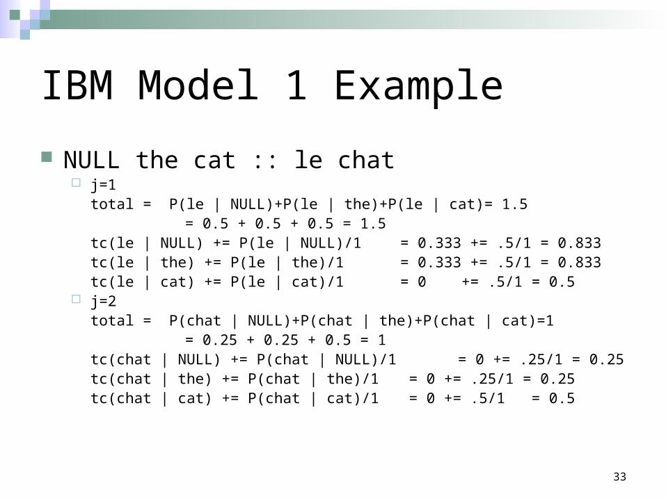
33

IBM Model 1 Example

NULL the cat :: le chat j=1

total = P(le | NULL)+P(le | the)+P(le | cat)= 1.5 = 0.5 + 0.5 + 0.5 = 1.5

tc(le | NULL) += P(le | NULL)/1 = 0.333 += .5/1 = 0.833tc(le | the) += P(le | the)/1 = 0.333 += .5/1 = 0.833tc(le | cat) += P(le | cat)/1 = 0 += .5/1 = 0.5

j=2total = P(chat | NULL)+P(chat | the)+P(chat | cat)=1

= 0.25 + 0.25 + 0.5 = 1tc(chat | NULL) += P(chat | NULL)/1 = 0 += .25/1 = 0.25tc(chat | the) += P(chat | the)/1 = 0 += .25/1 = 0.25tc(chat | cat) += P(chat | cat)/1 = 0 += .5/1 = 0.5

34

IBM Model 1 Example

Re-compute translations (iteration 2): total(the) = tc(le | the) + tc(chien | the) + tc(chat | the)

= .833 + 0.25 + 0.25 = 1.333 P(le | the) = tc(le | the)/total(the)

= .833 / 1.333 = 0.625 P(chien | the) = tc(chien | the)/total(the)

= 0.25/1.333 = 0.188 P(chat | the) = tc(chat | the)/total(the)

= 0.25/1.333 = 0.188 total(dog) = tc(le | dog) + tc(chien | dog) = 0.333 + 0.5 = 0.833 P(le | dog) = tc(le | dog)/total(dog)

= 0.333 / 0.833 = 0.4 P(chien | dog) = tc(chien | dog)/total(dog)

= 0.5 / 0.833 = 0.6

35

IBM Model 1Example

After 5 iterations: P(le | NULL) = 0.755608028335301 P(chien | NULL) = 0.122195985832349 P(chat | NULL) = 0.122195985832349 P(le | the) = 0.755608028335301 P(chien | the) = 0.122195985832349 P(chat | the) = 0.122195985832349 P(le | dog) = 0.161943319838057 P(chien | dog) = 0.838056680161943 P(le | cat) = 0.161943319838057 P(chat | cat) = 0.838056680161943

36

IBM Model 1 Recap

IBM Model 1 allows for an efficient computation of translation probabilities

No notion of fertility, i.e., it’s possible that the same English word is the best translation for all foreign words

No positional information, i.e., depending on the language pair, there might be a tendency that words occurring at the beginning of the English sentence are more likely to align to words at the beginning of the foreign sentence

37

IBM Model 3

IBM Model 3 offers two additional features compared to IBM Model 1:How likely is an English word e to align to k

foreign words (fertility)? Positional information (distortion), how likely is

a word in position i to align to a word in position j?

38

IBM Model 3: Fertility

The best Model 1 alignment could be that a single English word aligns to all foreign words

This is clearly not desirable and we want to constrain the number of words an English word can align to

Fertility models a probability distribution that word e aligns to k words: n(k,e)

Consequence: translation probabilities cannot be computed independently of each other anymore

IBM Model 3 has to work with full alignments, note there are up to (l+1)m different alignments

39

IBM Model 1 + Model 3

Iterating over all possible alignments is computationally infeasible

Solution: Compute the best alignment with Model 1 and change some of the alignments to generate a set of likely alignments (pegging)

Model 3 takes this restricted set of alignments as input

40

Pegging

Given an alignment a we can derive additional alignments from it by making small changes:Changing a link (j,i) to (j,i’)Swapping a pair of links (j,i) and (j’,i’) to (j,i’)

and (j’,i) The resulting set of alignments is called the

neighborhood of a

41

IBM Model 3: Distortion

The distortion factor determines how likely it is that an English word in position i aligns to a foreign word in position j, given the lengths of both sentences:

d(j | i, l, m) Note, positions are absolute positions

42

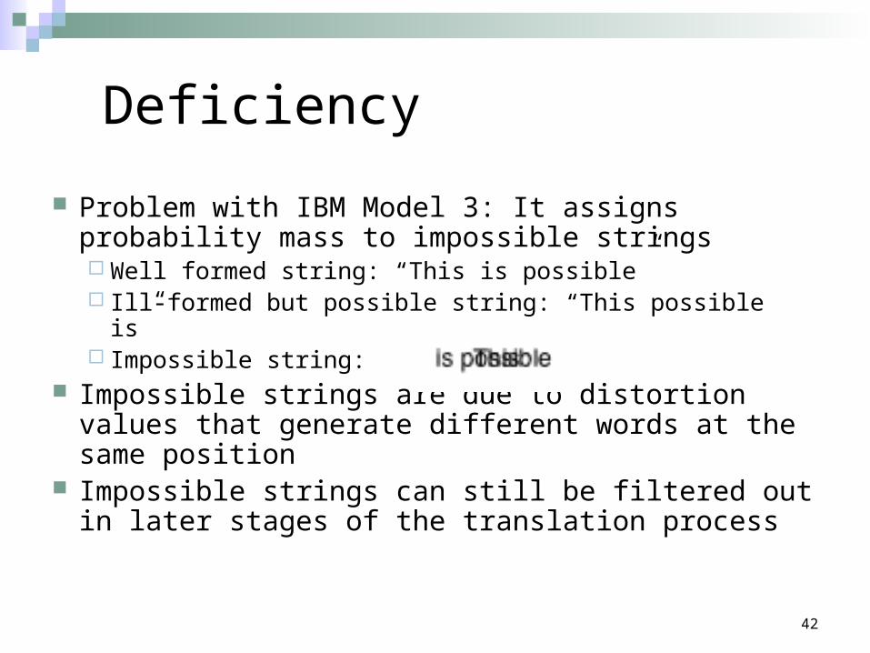
Deficiency

Problem with IBM Model 3: It assigns probability mass to impossible strings Well formed string: “This is possible” Ill-formed but possible string: “This possible is” Impossible string:

Impossible strings are due to distortion values that generate different words at the same position

Impossible strings can still be filtered out in later stages of the translation process

43

Limitations of IBM Models

Only 1-to-N word mapping Handling fertility-zero words (difficult for

decoding) Almost no syntactic information

Word classes Relative distortion

Long-distance word movement Fluency of the output depends entirely on the

English language model

44

Decoding

How to translate new sentences? A decoder uses the parameters learned on a parallel

corpus Translation probabilities Fertilities Distortions

In combination with a language model the decoder generates the most likely translation

Standard algorithms can be used to explore the search space (A*, greedy searching, …)

Similar to the traveling salesman problem