Statistical heartburn: An attempt to digest four pizza ... · Statistical heartburn: An attempt to...
19
Statistical heartburn: An attempt to digest four pizza publications from the Cornell Food and Brand Lab Tim van der Zee 1 , Jordan Anaya 2 , Nicholas J. L. Brown 3 1 Graduate School of Teaching (ICLON), Leiden University, Leiden, The Netherlands Email: [email protected] Twitter: @Research_Tim 2 Omnes Res, Charlottesville, Virginia, omnesres.com Email: [email protected] Twitter: @omnesresnetwork 3 University Medical Center, University of Groningen, The Netherlands Email: [email protected] Twitter: @sTeamTraen Corresponding Author: Nicholas J. L. Brown 3 PeerJ Preprints | https://doi.org/10.7287/peerj.preprints.2748v1 | CC BY 4.0 Open Access | rec: 25 Jan 2017, publ: 25 Jan 2017
Transcript of Statistical heartburn: An attempt to digest four pizza ... · Statistical heartburn: An attempt to...

Statistical heartburn: An attempt to digest four pizza
publications from the Cornell Food and Brand Lab
Tim van der Zee1, Jordan Anaya2, Nicholas J. L. Brown3
1 Graduate School of Teaching (ICLON), Leiden University, Leiden, The Netherlands
Email: [email protected]
Twitter: @Research_Tim
2 Omnes Res, Charlottesville, Virginia, omnesres.com
Email: [email protected]
Twitter: @omnesresnetwork
3 University Medical Center, University of Groningen, The Netherlands
Email: [email protected]
Twitter: @sTeamTraen
Corresponding Author:
Nicholas J. L. Brown3
PeerJ Preprints | https://doi.org/10.7287/peerj.preprints.2748v1 | CC BY 4.0 Open Access | rec: 25 Jan 2017, publ: 25 Jan 2017

Statistical heartburn: An attempt to digest four pizzapublications from the Cornell Food and Brand LabTim van der Zee1, Jordan Anaya2, and Nicholas J. L. Brown3
1Graduate School of Teaching (ICLON), Leiden University, Leiden, The Netherlands2Omnes Res, Charlottesville, Virginia3University Medical Center, University of Groningen, The Netherlands
Corresponding author:Nicholas J. L. Brown3
Email address: [email protected]
ABSTRACT
We present the initial results of a reanalysis of four articles from the Cornell Food and Brand Lab based on data collectedfrom diners at an Italian restaurant buffet. On a first glance at these articles, we immediately noticed a number ofapparent inconsistencies in the summary statistics. A thorough reading of the articles and careful reanalysis of the resultsrevealed additional problems. The sample sizes for the number of diners in each condition are incongruous both withinand between the four articles. In some cases, the degrees of freedom of between-participant test statistics are largerthan the sample size, which is impossible. Many of the computed F and t statistics are inconsistent with the reportedmeans and standard deviations. In some cases, the number of possible inconsistencies for a single statistic was suchthat we were unable to determine which of the components of that statistic were incorrect. We contacted the authors ofthe four articles, but they have thus far not agreed to share their data. The attached Appendix reports approximately 150inconsistencies in these four articles, which we were able to identify from the reported statistics alone. We hope that ouranalysis will encourage readers, using and extending the simple methods that we describe, to undertake their own effortsto verify published results, and that such initiatives will improve the accuracy and reproducibility of the scientific literature.
Keywords: Statistics, Reproducibility, Replication, Reanalysis
INTRODUCTION
Concerns have been raised about the reproducibility of scientific research (Ioannidis, 2005), with many recent concernsfocusing on psychological research (Open Science Collaboration, 2015). Commonly cited reasons for the reproducibilitycrisis include the use of small sample sizes leading to low statistical power (Schwarz and Clore, 2016), a culture ofquestionable research practices (John et al., 2012), and an incentive structure that rewards large numbers of publicationsreporting sensational findings with little penalty for being wrong (Bakker et al., 2012; Smaldino and McElreath, 2016).However, a number of recent articles lead us to question whether a certain fraction of non-reproducibility might be dueto simple reporting or calculation errors. The prevalence of errors in the p values associated with reported test statisticshas been estimated to be anywhere from around 18% to almost 50% (Bakker and Wicherts, 2011; Nuijten et al., 2015).Another study found at least one apparent error in something as simple as a reported mean in around 50% of the articles itsauthors examined (Brown and Heathers, 2016). Of course, it is possible for one or two elementary typos to occur duringthe drafting of an article, and an erroneous statistic due to a participant missing a response on an item can slip into even themost carefully proofread manuscript. However, the presence of a high number of errors in simple statistics might make thereader wonder what else might have been done in a less than rigorous fashion.
Here, we examine four articles from the same laboratory, which contain a remarkably high number of apparent errors andinconsistencies. Our attention was first drawn to this series of articles when the senior author wrote a blog post about the
PeerJ Preprints | https://doi.org/10.7287/peerj.preprints.2748v1 | CC BY 4.0 Open Access | rec: 25 Jan 2017, publ: 25 Jan 2017

context in which the articles came to be written (Wansink, 2016). When we followed the references to the articles cited inthat blog post we immediately noticed some apparent inconsistencies1. We therefore decided to perform a close reanalysisof the four articles that seemed to be closely related to each other, to see how many problems we could identify. A detailedlist of over 150 individual inconsistencies and other problems is given in the Appendix; within the text of this article wediscuss some of the overarching issues with the four target articles and the implications of what we found.
The articles in questionWe reanalyzed four articles by Ozge Sıgırcı, Brian Wansink, and their colleagues, which appear to be based on a singledata set from one field experiment (Just et al., 2014, 2015; Sıgırcı and Wansink, 2015; Kniffin et al., 2016). We will refer tothese articles with the following numbering:
1. Just, D. R., Sıgırcı, O., & Wansink, B. (2014). Lower buffet prices lead to less taste satisfaction. Journal of SensoryStudies, 29(5), 362–370. doi:10.1111/joss.12117
2. Just, D. R., Sıgırcı, O., & Wansink, B. (2015). Peak-end pizza: Prices delay evaluations of quality. Journal ofProduct & Brand Management, 24(7), 770–778. doi:10.1108/jpbm01-2015-0802
3. Kniffin, K. M., Sıgırcı, O., & Wansink, B. (2016). Eating heavily: Men eat more in the company of women.Evolutionary Psychological Science, 2(1), 38–46. doi:10.1007/s40806-015-0035-3
4. Sıgırcı, O., & Wansink, B. (2015). Low prices and high regret: how pricing influences regret at all-you-can-eatbuffets. BMC Nutrition, 1(1), 36. doi:10.1186/s40795-015-0030-x
Each of the four target articles describes what we believe to be the same field study. Apart from the blog post mentionedabove, which strongly implied that the data set is common to these four articles, we base this conclusion on the followingobservations:
• Articles 1, 2, and 4 state that the study took place at “Aiello’s Italian Restaurant, a restaurant mid-way betweenSyracuse and Binghamton, New York.” Article 3 describes the location, differently but not inconsistently, as “anItalian restaurant in Northeastern USA.”
• All four articles mention that the study took place over a two-week period. Articles 1, 2, and 4 further specify thatthis period was in the spring, with data being collected between 11:00 a.m. and 1:30 p.m., and with the weatherbeing overcast and chilly or rainy throughout the days of the study.
• All four articles describe the presence of an all-you-can-eat lunch buffet. Articles 1, 2, and 4 (but not 3) explain thatthe study used a randomized between-subjects design in which participants were given a flyer that entitled them topay either $4 or $8 for the lunch buffet and a free beverage. People who arrived in groups were all assigned to thesame coupon condition.
• Articles 1, 2, and 4 describe the buffet as consisting of pizza, salad, breadsticks, pasta, and soup. Article 3 mentions“pizza, salad, and side dishes.”
• All four articles mention that the number of people recruited was either 139 in total, or 133 adults. Article 1 reportsthat of 139 total participants, 6 were eliminated for being under 18 years of age, thus also giving a total of 133 adults.
• All four articles describe how participants were intercepted at the cash register and given a short questionnaire, whichasked for demographic information along with a variety of questions about their restaurant experience.
Given the identical setting, which is often described with identical sentences across the four articles, and the presence ofmany identical results in different articles (e.g., Table 1 has been copied verbatim between Articles 1 and 2), we concludethat these articles all describe the same field study. However, none of the articles mentions that they are based on the samedata set as their predecessors, even though they were published over a period of many months. We consider that this mayconstitute a breach of good publication ethics practice (Kirkman and Chen, 2011); it is important for the reader to knowthat other articles may exist based on the same data set, so that he or she may appropriately judge the independent claimsof each article.
1The blog post mentioned a total of five articles. Four of these, examined here, were on the same topic; the fifth was on an entirely different topic,and we have not examined it in detail.
2/18
PeerJ Preprints | https://doi.org/10.7287/peerj.preprints.2748v1 | CC BY 4.0 Open Access | rec: 25 Jan 2017, publ: 25 Jan 2017

Methods for identifying errorsNone of the four target articles provides a link to a public version of the data set. We wrote to the correspondingauthors of all four articles, asking explicitly for a copy of the data. We received only one reply, from the authors’ lab’s“Communications Specialist”; this reply did not address our request for the data and instead suggested that we conduct areplication of the study. We wrote back, emphasizing that we wished to check a number of apparent inconsistencies inthe articles, but after two weeks we still have not heard back. We note that the publisher of at least one of the four targetarticles, BioMed Central (Article 4 was published in BMC Nutrition), currently imposes an explicit requirement on authorsto share their data as a condition of publication: “Submission of a manuscript to a BioMed Central journal implies thatmaterials described in the manuscript, including all relevant raw data, will be freely available to any scientist wishing touse them for non-commercial purposes” (BMC, 2017). Fortunately, multiple techniques exist that can identify a number oferrors in reported statistics even without access to the original data.
Granularity errorsStatistics of discrete data are granular, with the effect that they can only take on certain values when rounded to any givennumber of decimal places (typically 2). When the granularity of the statistic is greater than the precision of the reportedvalues, it becomes possible to report values that are mathematically impossible. For example, if the data are reported asintegers, such as survey questions on a Likert-type scale, and the mean is reported to two decimal places (a precision of0.01), it is possible for reported means to be inconsistent if the sample size is below 100 (Brown and Heathers, 2016).Similarly, it is also possible for standard deviations (SDs) to be inconsistent, although the calculation of which values areconsistent or not is more complex (Anaya, 2016).
Almost all of the means and SDs in the four target articles were for (sub)sample sizes below 100 and reported to two decimalplaces, allowing us to scrutinize them with granularity testing. To do this, we used a web application that simultaneouslychecks means (GRIM) and standard deviations (GRIMMER), as explained by Anaya (2016); we also checked meansindependently using an Excel spreadsheet (available at https://osf.io/3fcbr). SDs were assumed to be sample (versuspopulation) SDs in all cases. We took a conservative approach to rounding, allowing potentially ambiguous values (e.g., amean of 0.125) to be rounded both up and down (Brown and Heathers, 2016).
P valuesWe performed an automated check of the consistency between test statistics and p values with statcheck (Epskamp andNuijten, 2015), which did not identify any errors in any of the four articles. However, it should be noted that statcheck wasunable to identify most of the test statistics (it does not search tables and can miss tests in the text that are not in the correctformat). Furthermore, statcheck only checks if the p value is consistent with the test statistic and degrees of freedom (DFs);it cannot check if the test statistic or DFs are themselves correct.
Test statisticsIt is possible to recalculate the test statistics from a t test or an ANOVA using only the per-cell sample sizes, means,and standard deviations. The rpsychi package in R (R Core Team, 2016) provides functions to do this for one- andtwo-way ANOVAs (a one-way ANOVA with two groups is equivalent to a t test, with the F statistic being the square of thet statistic).
To account for uncertainty in the recalculation of the test statistics due to errors introduced by the rounding of the re-ported means and SDs on which these statistics were based, we calculated upper and lower bounds for the test statistics,and treated reported statistics in the target articles as valid if they fell within these bounds. We calculated the upperbound of each F (or, in a few cases, t) statistic by subtracting .005 from all of the SDs (thus biasing all of the standarderrors downward) and then generating every combination of the means with .005 either added to or subtracted fromeach, retaining the largest test statistic produced by all of these combinations. For the lower bound, we performed theanalogous operations in reverse, adding .005 to each of the SDs and retaining the smallest test statistic from every setof means that had been adjusted by either the addition or subtraction of .005 to each value. Because we used all ofthe most extreme possible values from which the means and SDs could have been rounded, we believe that our reanal-
3/18
PeerJ Preprints | https://doi.org/10.7287/peerj.preprints.2748v1 | CC BY 4.0 Open Access | rec: 25 Jan 2017, publ: 25 Jan 2017
ysis gives a conservative estimate of the number of inconsistencies in the F and t statistics reported in the four target articles.
As well as the bounds for the F and t statistics, we also recalculated p values wherever this was possible and appropriate.All of the recalculations were performed separately by the second and third authors in Python and in R, respectively, andchecked by all authors. We copied and pasted the means and SDs from the published tables into a text editor and thentransformed these numbers to data structures in the programming languages that we were using, in order to avoid possiblecorruption due to typing errors on our part. The code for our calculations is available in the GitHub repository associatedwith the present article.
MAJOR CONCERNS
Here we will go over some observations we made which both raise serious questions about the integrity of the data set usedin these papers, and the accuracy of the report.
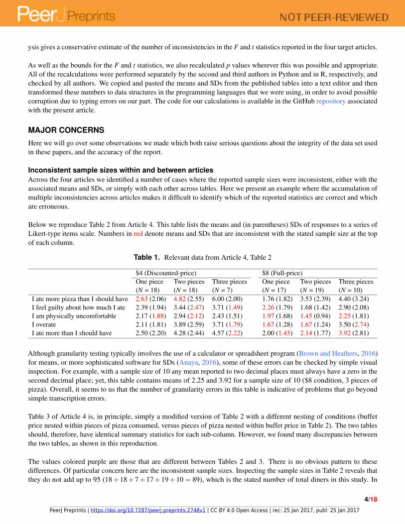
Inconsistent sample sizes within and between articlesAcross the four articles we identified a number of cases where the reported sample sizes were inconsistent, either with theassociated means and SDs, or simply with each other across tables. Here we present an example where the accumulation ofmultiple inconsistencies across articles makes it difficult to identify which of the reported statistics are correct and whichare erroneous.
Below we reproduce Table 2 from Article 4. This table lists the means and (in parentheses) SDs of responses to a series ofLikert-type items scale. Numbers in red denote means and SDs that are inconsistent with the stated sample size at the topof each column.
Table 1. Relevant data from Article 4, Table 2
$4 (Discounted-price) $8 (Full-price)One piece Two pieces Three pieces One piece Two pieces Three pieces(N = 18) (N = 18) (N = 7) (N = 17) (N = 19) (N = 10)
I ate more pizza than I should have 2.63 (2.06) 4.82 (2.55) 6.00 (2.00) 1.76 (1.82) 3.53 (2.39) 4.40 (3.24)I feel guilty about how much I ate 2.39 (1.94) 3.44 (2.47) 3.71 (1.49) 2.26 (1.79) 1.68 (1.42) 2.90 (2.08)I am physically uncomfortable 2.17 (1.88) 2.94 (2.12) 2.43 (1.51) 1.97 (1.68) 1.45 (0.94) 2.25 (1.81)I overate 2.11 (1.81) 3.89 (2.59) 3.71 (1.79) 1.67 (1.28) 1.67 (1.24) 3.50 (2.74)I ate more than I should have 2.50 (2.20) 4.28 (2.44) 4.57 (2.22) 2.00 (1.45) 2.14 (1.77) 3.92 (2.81)
Although granularity testing typically involves the use of a calculator or spreadsheet program (Brown and Heathers, 2016)for means, or more sophisticated software for SDs (Anaya, 2016), some of these errors can be checked by simple visualinspection. For example, with a sample size of 10 any mean reported to two decimal places must always have a zero in thesecond decimal place; yet, this table contains means of 2.25 and 3.92 for a sample size of 10 ($8 condition, 3 pieces ofpizza). Overall, it seems to us that the number of granularity errors in this table is indicative of problems that go beyondsimple transcription errors.
Table 3 of Article 4 is, in principle, simply a modified version of Table 2 with a different nesting of conditions (buffetprice nested within pieces of pizza consumed, versus pieces of pizza nested within buffet price in Table 2). The two tablesshould, therefore, have identical summary statistics for each sub-column. However, we found many discrepancies betweenthe two tables, as shown in this reproduction.
The values colored purple are those that are different between Tables 2 and 3. There is no obvious pattern to thesedifferences. Of particular concern here are the inconsistent sample sizes. Inspecting the sample sizes in Table 2 reveals thatthey do not add up to 95 (18+18+7+17+19+10 = 89), which is the stated number of total diners in this study. In
4/18
PeerJ Preprints | https://doi.org/10.7287/peerj.preprints.2748v1 | CC BY 4.0 Open Access | rec: 25 Jan 2017, publ: 25 Jan 2017
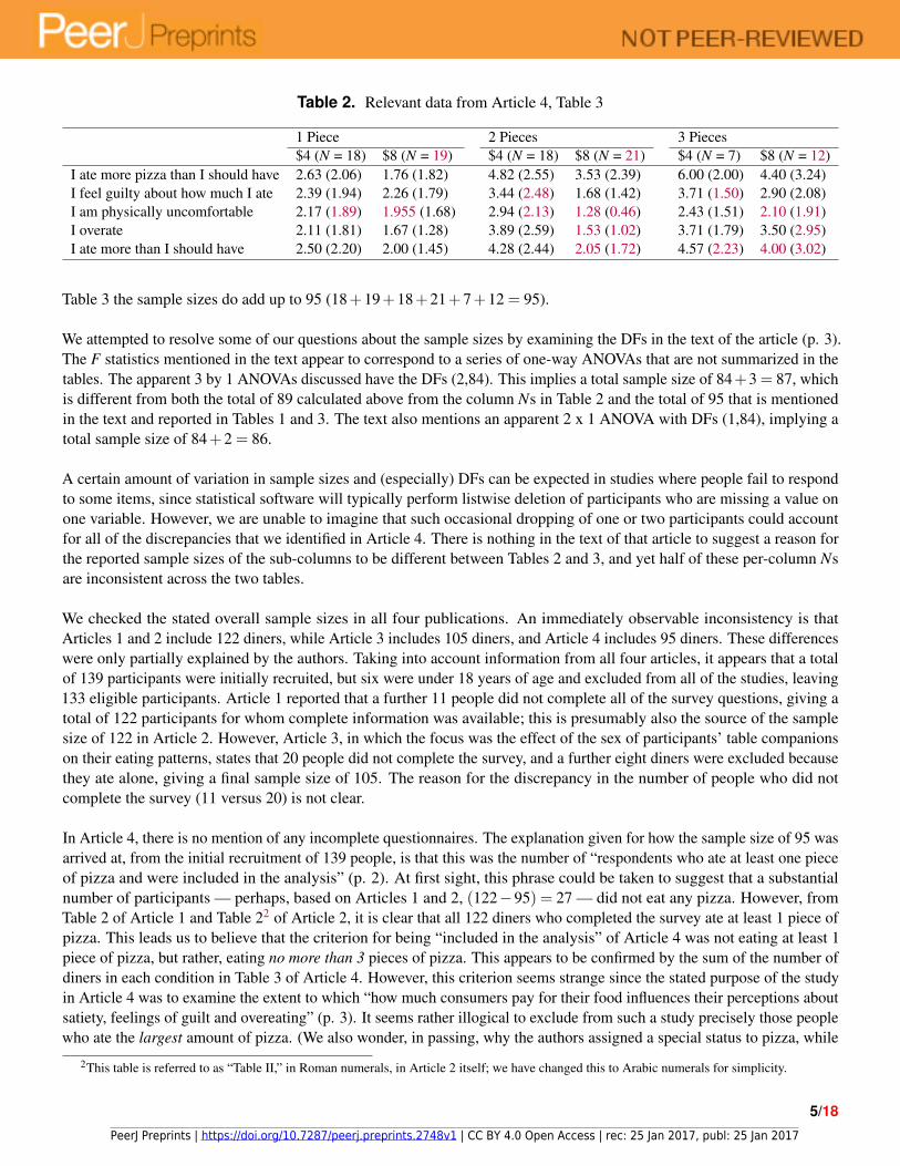
Table 2. Relevant data from Article 4, Table 3
1 Piece 2 Pieces 3 Pieces$4 (N = 18) $8 (N = 19) $4 (N = 18) $8 (N = 21) $4 (N = 7) $8 (N = 12)
I ate more pizza than I should have 2.63 (2.06) 1.76 (1.82) 4.82 (2.55) 3.53 (2.39) 6.00 (2.00) 4.40 (3.24)I feel guilty about how much I ate 2.39 (1.94) 2.26 (1.79) 3.44 (2.48) 1.68 (1.42) 3.71 (1.50) 2.90 (2.08)I am physically uncomfortable 2.17 (1.89) 1.955 (1.68) 2.94 (2.13) 1.28 (0.46) 2.43 (1.51) 2.10 (1.91)I overate 2.11 (1.81) 1.67 (1.28) 3.89 (2.59) 1.53 (1.02) 3.71 (1.79) 3.50 (2.95)I ate more than I should have 2.50 (2.20) 2.00 (1.45) 4.28 (2.44) 2.05 (1.72) 4.57 (2.23) 4.00 (3.02)
Table 3 the sample sizes do add up to 95 (18+19+18+21+7+12 = 95).
We attempted to resolve some of our questions about the sample sizes by examining the DFs in the text of the article (p. 3).The F statistics mentioned in the text appear to correspond to a series of one-way ANOVAs that are not summarized in thetables. The apparent 3 by 1 ANOVAs discussed have the DFs (2,84). This implies a total sample size of 84+3 = 87, whichis different from both the total of 89 calculated above from the column Ns in Table 2 and the total of 95 that is mentionedin the text and reported in Tables 1 and 3. The text also mentions an apparent 2 x 1 ANOVA with DFs (1,84), implying atotal sample size of 84+2 = 86.
A certain amount of variation in sample sizes and (especially) DFs can be expected in studies where people fail to respondto some items, since statistical software will typically perform listwise deletion of participants who are missing a value onone variable. However, we are unable to imagine that such occasional dropping of one or two participants could accountfor all of the discrepancies that we identified in Article 4. There is nothing in the text of that article to suggest a reason forthe reported sample sizes of the sub-columns to be different between Tables 2 and 3, and yet half of these per-column Nsare inconsistent across the two tables.
We checked the stated overall sample sizes in all four publications. An immediately observable inconsistency is thatArticles 1 and 2 include 122 diners, while Article 3 includes 105 diners, and Article 4 includes 95 diners. These differenceswere only partially explained by the authors. Taking into account information from all four articles, it appears that a totalof 139 participants were initially recruited, but six were under 18 years of age and excluded from all of the studies, leaving133 eligible participants. Article 1 reported that a further 11 people did not complete all of the survey questions, giving atotal of 122 participants for whom complete information was available; this is presumably also the source of the samplesize of 122 in Article 2. However, Article 3, in which the focus was the effect of the sex of participants’ table companionson their eating patterns, states that 20 people did not complete the survey, and a further eight diners were excluded becausethey ate alone, giving a final sample size of 105. The reason for the discrepancy in the number of people who did notcomplete the survey (11 versus 20) is not clear.
In Article 4, there is no mention of any incomplete questionnaires. The explanation given for how the sample size of 95 wasarrived at, from the initial recruitment of 139 people, is that this was the number of “respondents who ate at least one pieceof pizza and were included in the analysis” (p. 2). At first sight, this phrase could be taken to suggest that a substantialnumber of participants — perhaps, based on Articles 1 and 2, (122−95) = 27 — did not eat any pizza. However, fromTable 2 of Article 1 and Table 22 of Article 2, it is clear that all 122 diners who completed the survey ate at least 1 piece ofpizza. This leads us to believe that the criterion for being “included in the analysis” of Article 4 was not eating at least 1piece of pizza, but rather, eating no more than 3 pieces of pizza. This appears to be confirmed by the sum of the number ofdiners in each condition in Table 3 of Article 4. However, this criterion seems strange since the stated purpose of the studyin Article 4 was to examine the extent to which “how much consumers pay for their food influences their perceptions aboutsatiety, feelings of guilt and overeating” (p. 3). It seems rather illogical to exclude from such a study precisely those peoplewho ate the largest amount of pizza. (We also wonder, in passing, why the authors assigned a special status to pizza, while
2This table is referred to as “Table II,” in Roman numerals, in Article 2 itself; we have changed this to Arabic numerals for simplicity.
5/18
PeerJ Preprints | https://doi.org/10.7287/peerj.preprints.2748v1 | CC BY 4.0 Open Access | rec: 25 Jan 2017, publ: 25 Jan 2017

apparently ignoring the effect that consumption of another high-calorie food such as pasta might have on diners’ feelingsabout overeating. That is, those who ate no or just one pizza slice might have eaten much more of other food types, whichseems relevant for a study on overeating.)
We continued our analyses of the sample sizes to determine how many people in each price condition (i.e., paying either $4or $8 for the buffet) ate each number of slices3 of pizza. We started this process in Table 2 of Article 2, which providesstatistics for different linear regression models predicting variance in diners’ overall satisfaction with the pizza that they atefrom their satisfaction with each slice.
Table 3. Relevant data from Article 2, Table 2
Half price ($4) Full price ($8)Models Models
Beginning Total End Peak Peak-end Beginning Total End Peak Peak-endN = 62 N = 41 N = 47 N = 62 N = 47 N = 60 N = 26 N = 38 N = 60 N = 38
Here, the “Beginning” model is built with information regarding the first slice of pizza that each diner ate. The “End”model is built with information regarding the last slice that each diner ate, provided they ate at least 2 slices. The “Total”model contains, for diners who ate at least 3 slices, ratings of the first slice, middle slice (or one of the pair of slices oneither side of the “midpoint”, if the total number of slices was even), and last slice. That is:
• The “Beginning” model contains all diners who ate at least 1 slice• The “End” model contains all diners who ate at least 2 slices• The “Total” model contains all diners who ate at least 3 slices
With this information it follows that at the $4 price point:
62 diners ate 1 or more slices, 47 diners ate 2 or more slices, and 41 diners ate 3 or more slices
From which we can deduce:
62−47 = 15 diners ate 1 slice, 47−41 = 6 diners ate 2 slices, and 41 diners ate 3 or more slices
Similarly, at the $8 price point:
60 diners ate 1 or more slices, 38 diners ate 2 or more slices, and 26 diners ate 3 or more slices
From which we can deduce:
60−38 = 22 diners ate 1 slice, 38−26 = 12 diners ate 2 slices, and 26 diners ate 3 or more slices
We were able to compare these per-condition sample sizes for people who ate exactly 1 or 2 slices with the equivalentnumbers from Table 3 of Article 4. (We chose Table 3, rather than Table 2, because the per-column sample sizes in Table 3are consistent with the overall sample size of 95 for that study.) Our Table 4 shows the sample sizes, which are all differentbetween the two articles. Additionally, the sample in Article 4 appears to be a subset of the sample from Article 2 (withpeople who ate more than 3 slices of pizza excluded); as a result, it should not be possible for any of the groups in Article 4to be larger than the equivalent group in Article 2. However, three out of the four groups are larger in Article 4 than inArticle 2. Even if the diners in Article 4 are not a subset of those in Article 2 (for example, because the 11 diners who wereexcluded from Article 2 for having incomplete questionnaires were included in Article 4, and all 11 of those diners ateexactly 2 slices of pizza), this is insufficient to explain the number of people reported as eating exactly 2 slices of pizza in
6/18
PeerJ Preprints | https://doi.org/10.7287/peerj.preprints.2748v1 | CC BY 4.0 Open Access | rec: 25 Jan 2017, publ: 25 Jan 2017
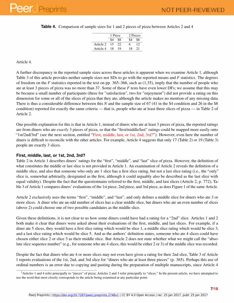
Table 4. Comparison of sample sizes for 1 and 2 pieces of pizza between Articles 2 and 4
1 Piece 2 Pieces$4 $8 $4 $8
Article 2 15 22 6 12Article 4 18 19 18 21
Article 4.
A further discrepancy in the reported sample sizes across these articles is apparent when we examine Article 1, althoughTable 3 of this article provides neither sample sizes nor SDs to go with the reported means and F statistics. The degreesof freedom on the F statistics reported in the text on pp. 365–366, such as (1,35), imply that the number of people whoate at least 3 pieces of pizza was no more than 37. Some of these F tests have even lower DFs; we assume that this maybe because a small number of participants (three for ”satisfaction”, two for ”enjoyment”) did not provide a rating on thisdimension for some or all of the slices of pizza that they ate, although the article makes no mention of any missing data.There is thus a considerable difference between this N and the sample size of 67 (41 in the $4 condition and 26 in the $8condition) reported for exactly the same criteria — that is, people who ate at least three slices of pizza — in Table 2 ofArticle 2.
One possible explanation for this is that in Article 1, instead of diners who ate at least 3 pieces of pizza, the reported ratingsare from diners who ate exactly 3 pieces of pizza, so that the “first/middle/last” ratings could be mapped more easily onto“1st/2nd/3rd” (see the next section, entitled “First, middle, last, or 1st, 2nd, 3rd?”). However, even here the number ofdiners is difficult to reconcile with the other articles. For example, Article 4 suggests that only 17 (Table 2) or 19 (Table 3)people ate exactly 3 slices.
First, middle, last, or 1st, 2nd, 3rd?Table 2 in Article 1 describes diners’ ratings for the “first”, “middle”, and “last” slice of pizza. However, the definition ofwhat constitutes the middle or last slice is not provided in Article 1. An examination of Article 2 reveals the definition of amiddle slice, and also that someone who only ate 1 slice has a first slice rating, but not a last slice rating (i.e., the “only”slice is, somewhat arbitrarily, designated as the first, although it could arguably also be described as the last slice withequal validity). Despite the fact that the questionnaire referred to the first, middle, and last slices (Article 2, p. 772), Ta-ble 3 of Article 1 compares diners’ evaluations of the 1st piece, 2nd piece, and 3rd piece, as does Figure 1 of the same Article.
Article 2 exclusively uses the terms “first”, “middle”, and “last”, and only defines a middle slice for diners who ate 3 ormore slices. A diner who ate an odd number of slices has a clear middle slice, but diners who ate an even number of slices(above 2) could choose one of two possible candidates as the middle slice.
Given these definitions, it is not clear to us how some diners could have had a rating for a “2nd” slice. Articles 1 and 2both make it clear that diners were asked about their evaluations of the first, middle, and last slices. For example, if adiner ate 5 slices, they would have a first slice rating which would be slice 1, a middle slice rating which would be slice 3,and a last slice rating which would be slice 5. And as the authors’ definition states, someone who ate 4 slices could havechosen either slice 2 or slice 3 as their middle slice. But Article 2 does not state whether what we might call the “abso-lute slice sequence number” (e.g., for someone who ate 4 slices, this would be either 2 or 3) of the middle slice was recorded.
Despite the fact that diners who ate 4 or more slices may not even have given a rating for their 2nd slice, Table 3 of Article1 reports evaluations of the 1st, 2nd, and 3rd slice for “diners who ate at least three pieces” (p. 365). Perhaps this use ofordinal numbers is an error due to copying and pasting during the preparation of multiple manuscripts, since Article 4
3Articles 1 and 4 refer principally to “pieces” of pizza; Articles 2 and 3 refer principally to “slices.” In the present article, we have attempted touse the word that most closely corresponds to the article being examined at any particular point.
7/18
PeerJ Preprints | https://doi.org/10.7287/peerj.preprints.2748v1 | CC BY 4.0 Open Access | rec: 25 Jan 2017, publ: 25 Jan 2017
discusses diners who ate 1, 2, or 3 slices of pizza; it could be that in Table 3 of Article 1, and the discussion around it, theterms “1st,” “2nd,” and “3rd” should have read “first,” “middle,” and “last.” But if this were the case, then Figure 1A ofArticle 1 ought to show identical results to Figure 1 of Article 2; however, these figures differ in several ways (for example,the rating for the taste of the last slice in the $4 condition is 6.10 in Figure 1 of Article 2, but the bar in Figure 1A of Article1, and the corresponding entry in Table 3 of Article 1, shows a value of 6.38). As a result, it is unclear to us exactly whatdata are presented in Table 3 and Figure 1 of Article 1.
Further investigation into Articles 1 and 2 only adds to the confusion. On page 772 of Article 2 the authors use the DFs(2,80) and (2,50) to test the effect of slice order (first, middle, last) on pizza evaluations for the half price and full pricegroups, respectively. These DFs are correct assuming a repeated measures design and taking the sample sizes from the“total” models (41 and 26) in Table 2 of Article 2. In turn, this implies that Figure 1 of Article 2 shows the evaluations ofdiners who ate 3 or more slices of pizza. While someone who ate a first slice could have consumed 1, 2, 3, or more slices,anyone who ate a middle slice ate 3 or more slices (by definition); as a result we should be able to obtain the “taste ofmiddle slice” value for Figure 1 of Article 2 from Table 2 of Article 1. The value for the half-price ($4) group from Table 2of Article 1 is 6.68, which matches 6.68 in Figure 1 of Article 2. However, the value for the full-price ($8) group of 7.97 inTable 2 of Article 1 does not match the value of 8.00 in Figure 1 of Article 2.
Further inconsistencies across studiesAssuming that all four articles do indeed describe studies using the same participants and the same data collectionprocedures, there appear to be further inconsistencies in the reporting of the methods and results across the four articles.For example:
1. Article 3 describes how researchers observed the diners during their meal in order to establish how many slicesof pizza and bowls of salad each person ate, including “appropriate subtractions” (p. 41) for unfinished slices ofpizza and bowls of salad when these were cleaned away by waitstaff. However, none of the other articles gives anyindication that the number of slices of pizza consumed was anything but an integer. Additionally, Article 2 states thatthe researchers were “not able to accurately measure consumption of non-pizza food items” (p. 772) — a statementthat might refer to an inability to count fractional portions, or simply explain the article’s exclusive focus on pizza,but which in any case directly contradicts Article 3, which included data for how much salad was consumed. Article2 also claims that “pizza was by far the most popular choice on the buffet”; however, Table 2 in Article 3 indicatesthat more bowls of salad were consumed than slices of pizza for every group, and sometimes by a wide margin (e.g.,4.83 bowls of salad vs. 1.33 pizza slices for females eating with males).
2. Articles 1, 2, and 4 all state that the modal number of slices of pizza consumed by each participant was three.However, the numbers of participants who were reported to have consumed each number of slices varies considerablybetween these articles. In Article 1, the DFs on pp. 365–366 suggest that 37 people (see previous discussion) atethree or more slices, and the per-column Ns of Table 2 show that 122 people ate at least 1 slice, meaning that(122−37 = 85) people ate either 1 or 2 slices. However this number might be partitioned between those who ate 1and 2 slices, at least one of the components will be 43 or larger (i.e., greater than the 37 people who ate 3 slices), sothe modal number of slices must be either 1 or 2. In Article 4, the claim that the modal number of slices was 3 isdirectly contradicted by the sub-column headings in Tables 2 and 3, regardless of how the inconsistencies betweenthese two tables are resolved (see also the section above). Only in Article 2 is it possible for the modal number ofslices of pizza consumed to have been 3, given the reported sample sizes. Thus, either the modal number of slicesconsumed was different between studies and has been reported incorrectly in at least one case (which would be aninteresting result, given all the evidence that these four articles almost certainly come from the same data set), or thenumbers of participants who ate each number of slices of pizza are incorrectly reported by a wide margin in at leasttwo articles.
8/18
PeerJ Preprints | https://doi.org/10.7287/peerj.preprints.2748v1 | CC BY 4.0 Open Access | rec: 25 Jan 2017, publ: 25 Jan 2017

DISCUSSION
Here, we have presented in-depth reanalyses of four published articles from the same laboratory that reported a varietyof analyses of what appeared to be the same data set, gathered in the field setting of an all-you-can-eat buffet restaurant.We have shown that these articles contain a very large number of apparent errors and inconsistencies. The types of errorsinclude: impossible sample sizes within and between articles, incorrectly calculated and/or reported test statistics anddegrees of freedom, and a large number of impossible means and standard deviations. In total, we over 150 inconsistenciesand impossibilities in these four papers. Taken together, these problems make it difficult to have confidence in the authors’conclusions.
In examining these articles we were conservative with our methods and tried to give the authors the benefit of the doubt atall stages. We made generous allowances for rounding, considered all possibilities for test statistics, and made multiplepasses within and across the articles to try and identify the correct sample sizes. We checked granularity errors withan online web application, with an Excel sheet, with R code, and by hand. Two of us reconstructed the test statisticswith two different programming languages and multiple statistical packages and formulas, and in some cases with onlineapplications as well. We consulted several sources to ensure that we understood the correct degrees of freedom for all thetests that appeared to have been performed by the original authors (most statistics are not accompanied by any informationas to what was being measured). We constructed test data sets and checked our methods with these.
None of us can remember encountering a set of articles with as many inconsistencies and unresolved questions in the basicreporting of results as in this case. Our best guess as to what might have happened is that the four articles started out as onesingle project and some wires became crossed when this project was being sliced up into publishable units. This mightexplain the strange mixture of “first,” “middle,” and “last” slices with “1st,” “2nd,” and “3rd” in Article 1, with both ofthose sequences only being defined in other articles in the series.
A full explanation of what took place would probably require a substantial amount of input from the authors of the fourtarget articles. It will certainly require access to the data set; however, our attempts to obtain the data have been unsuccessfuluntil now (this preprint was submitted on January 24, 2017)4. Until such an explanation is forthcoming, we suggest that theresearch community may wish to exercise caution in interpreting the results presented in the four target articles.
We noted earlier that our attention was drawn to this series of articles by a blog post written by the senior author (Wansink,2016). Reactions by readers of that blog post mostly fell into one of two categories. Some were critical of the hiring andmanagement policies of the laboratory that they felt were implied by the blog post, while others expressed skepticism aboutthe ways in which the hypotheses tested by the researchers were generated. Although we have our own feelings aboutboth of these issues, we have chosen to concentrate here only on the objective problems that we identified in the publishedliterature, in the hope that the record will be corrected by whatever means the authors and the respective journal editorsmight consider appropriate. After all, as the aforementioned blog post stated, the resume of one of the authors will alwayshave these papers on it.
CONCLUSION
Science cannot be expected to always be “correct”, but it is expected to be done carefully and accurately. This is essentialbecause science builds upon itself, and without a solid foundation future studies are doomed to fail; the cumulative advancesin knowledge required for true progress are only possible when the scientific literature is trustworthy and accurate.Using the discussed papers as an example, the present work contributes to this goal by:
4When we wrote to the original authors to ask for their data, they proposed that we either conduct a replication of their study instead, or enterinto an agreement with them to license their data for use in our own original analyses (apparently in the belief that we were interested in learningmore about patterns of pizza consumption). When we explained that we wanted to see the data in order to check what appeared to be a number ofinconsistencies in their studies, we received no further reply (it has been two weeks since our last email).
9/18
PeerJ Preprints | https://doi.org/10.7287/peerj.preprints.2748v1 | CC BY 4.0 Open Access | rec: 25 Jan 2017, publ: 25 Jan 2017

1. Raising awareness that the published literature is not flawless, and that these flaws can include gross inconsistenciesand impossibilities
2. Showing that many such errors can be analyzed effectively without direct access to the original data with varioustools
3. Calling upon the scientific community — both editors and reviewers prior to publication of an article, and readers ingeneral after publication — to more closely scrutinize reported results in the literature
The first and third of these points have been investigated and discussed before in various publications (Ioannidis, 2005;Open Science Collaboration, 2015; John et al., 2012; Bakker and Wicherts, 2011; Nuijten et al., 2015; Brown and Heathers,2016). However, relatively little attention has been given to the second point, namely how critical readers can scrutinizereported results in the literature, and what tools are available for this purpose. In this paper we have demonstratedvarious such tools, which allow a critical appreciation of the veracity of reported results even without direct access to thedata. These tools can be used in additional to the readers’ more qualitative judgment of a paper, such as regarding theappropriateness of sampling or choice of statistical tests. Much of the value of these tools lies in their objectivity, as theytest the mathematical plausibility of reported results. We think that the existence and usage of these tools ought to be morewidely known among authors, editors, reviewers, and anyone who “merely” reads the published literature.
Although there is arguably no one-size-fits-all approach when it comes to checking papers, there are a variety of standardsteps that can be used with many studies. Manual inspection can reveal inconsistencies in reported sample sizes within apaper, or between multiple papers based on the same data. These checks should also include inspection of reported degreesof freedom, which are straightforward to calculate for common analyses such as t tests and ANOVAs. Subsequently,statcheck, and various other online tools, allow the critical reader to easily check common statistics such as z, t, and F testseither one by one (GraphPad, 2017; Stangroom, 2017; StatTrek.com, 2017) or en masse (Epskamp and Nuijten, 2015).In addition, any mean or SD based on granular data (such as Likert-type measures) can be checked for plausibility usingGRIMMER (Anaya, 2016). A most relevant application is that to statistics describing Likert-type data, which are verycommon in the social sciences. Note that none of the tests mentioned above are limited to values reported in texts or tables;visualizations such as charts or path diagrams should also be carefully inspected.
It is important to consider that all these tests can do is assess the accuracy of reported results, which may or may not reflectthe veracity of the underlying data or the appropriateness of the analyses that were performed. Even the most conscientiousresearcher will undoubtedly make mistakes from time to time. As such, we suggest that these tests be interpreted carefullyand conservatively, and readers should take into account the number and types of any set of inconsistencies. On the otherhand, even when reported results were generated by a completely random process, some of them will not be detected asbeing inconsistent by tools like statcheck and GRIM/GRIMMER. That is, these tests may not only give false positives insome cases (typos and other innocent errors), but also false negatives (failing to detect a true inconsistency). For example, ifa mean of 4.28 with a sample size of 58 is misreported as 4.27, this will be detected by GRIM (Brown and Heathers, 2016),but if the misreported value were 4.26, this would appear to be consistent. This added uncertainty should be consideredwhen interpreting the range of inconsistencies, or lack thereof. All in all, these tools can be powerful aids to the criticalexamination of published results, but their output should always be interpreted with caution.
Finally, we want to emphasize that a critical inspection of the published literature should not be mischaracterized as ahobby for the overly cynical, nor as so-called “methodological terrorism”. On the contrary, carefully evaluating presenteddata is a cornerstone of scientific investigation, and it is only logical to apply this also to the published literature. If we arenot willing to critically assess published studies, we also cannot guarantee their veracity.
APPENDIX: LIST OF INCONSISTENCIESThe following is a list of inconsistencies that we noticed and verified mathematically in the four publications. This list maynot be exhaustive, as not all statistics could be checked without the data set and more details of the methods that wereused. Sample sizes listed in the publications were taken at face value except for lines 5–10 of Article 1, Table 2, where it is
10/18
PeerJ Preprints | https://doi.org/10.7287/peerj.preprints.2748v1 | CC BY 4.0 Open Access | rec: 25 Jan 2017, publ: 25 Jan 2017
clear from Article 2 that different numbers of diners have first slice, middle slice, and last slice data. We have no way ofknowing whether the inconsistencies we identified are typos or calculation errors.
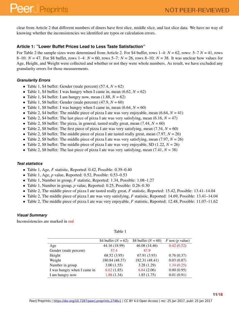
Article 1: ”Lower Buffet Prices Lead to Less Taste Satisfaction”For Table 2 the sample sizes were determined from Article 2. For $4 buffet, rows 1–4: N = 62, rows: 5–7 N = 41, rows8–10: N = 47. For $8 buffet, rows 1–4: N = 60, rows 5–7: N = 26, rows 8–10: N = 38. It was unclear how values forAge, Height, and Weight were collected and whether or not they were whole numbers. As result, we have excluded anygranularity errors for those measurements.
Granularity Errors
• Table 1, $4 buffet: Gender (male percent) (57.4, N = 62)• Table 1, $4 buffet: I was hungry when I came in, mean (6.62, N = 62)• Table 1, $4 buffet: I am hungry now, mean (1.88, N = 62)• Table 1, $8 buffet: Gender (male percent) (47.9, N = 60)• Table 1, $8 buffet: I was hungry when I came in, mean (6.64, N = 60)• Table 2, $4 buffet: The middle piece of pizza I ate was very enjoyable, mean (6.64, N = 41)• Table 2, $4 buffet: The last piece of pizza I ate was very satisfying, mean (6.16, N = 47)• Table 2, $8 buffet: The pizza, in general, tasted really great, mean (7.44, N = 60)• Table 2, $8 buffet: The first piece of pizza I ate was very satisfying, mean (7.34, N = 60)• Table 2, $8 buffet: The middle piece of pizza I ate tasted really great, mean (7.97, N = 26)• Table 2, $8 buffet: The middle piece of pizza I ate was very satisfying, mean (7.97, N = 26)• Table 2, $8 buffet: The middle piece of pizza I ate was very enjoyable, SD (1.22, N = 26)• Table 2, $8 buffet: The last piece of pizza I ate was very satisfying, mean (7.41, N = 38)
Test statistics
• Table 1, Age, F statistic, Reported: 0.42, Possible: 0.39–0.40• Table 1, Age, p value, Reported: 0.52, Possible: 0.53–0.53• Table 1, Number in group, F statistic, Reported: 1.34, Possible: 1.08–1.27• Table 1, Number in group, p value, Reported: 0.25, Possible: 0.26–0.30• Table 2, The middle piece of pizza I ate tasted really great, F statistic, Reported: 15.42, Possible: 13.41–14.04• Table 2, The middle piece of pizza I ate was very satisfying, F statistic, Reported: 14.69, Possible: 13.41–14.04• Table 2, The middle piece of pizza I ate was very enjoyable, F statistic, Reported: 12.48, Possible: 11.07–11.62
Visual Summary
Inconsistencies are marked in red
Table 1
$4 buffet (N = 62) $8 buffet (N = 60) F test (p value)Age 44.16 (18.99) 46.08 (14.46) 0.42 (0.52)Gender (male percent) 57.4 47.9Height 68.52 (3.95) 67.91 (3.93) 0.76 (0.37)Weight 180.84 (48.37) 182.31 (48.41) 0.03 (0.87)Number in group 3.00 (1.55) 3.28 (1.29) 1.34 (0.25)I was hungry when I came in 6.62 (1.85) 6.64 (2.06) 0.00 (0.95)I am hungry now 1.88 (1.34) 1.85 (1.75) 0.01 (0.91)
11/18
PeerJ Preprints | https://doi.org/10.7287/peerj.preprints.2748v1 | CC BY 4.0 Open Access | rec: 25 Jan 2017, publ: 25 Jan 2017
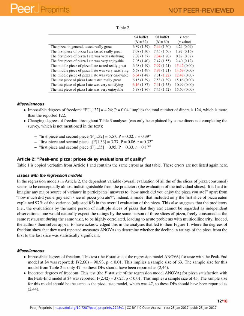
Table 2
$4 buffet $8 buffet F test(N = 62) (N = 60) (p value)
The pizza, in general, tasted really great 6.89 (1.39) 7.44 (1.60) 4.24 (0.04)The first piece of pizza I ate tasted really great 7.08 (1.30) 7.45 (1.60) 1.97 (0.16)The first piece of pizza I ate was very satisfying 7.08 (1.37) 7.34 (1.70) 0.82 (0.37)The first piece of pizza I ate was very enjoyable 7.05 (1.40) 7.47 (1.55) 2.40 (0.12)The middle piece of pizza I ate tasted really great 6.68 (1.49) 7.97 (1.21) 15.42 (0.00)The middle piece of pizza I ate was very satisfying 6.68 (1.49) 7.97 (1.21) 14.69 (0.00)The middle piece of pizza I ate was very enjoyable 6.64 (1.48) 7.81 (1.22) 12.48 (0.00)The last piece of pizza I ate tasted really great 6.15 (1.89) 7.58 (1.39) 15.16 (0.00)The last piece of pizza I ate was very satisfying 6.16 (1.87) 7.41 (1.55) 10.99 (0.00)The last piece of pizza I ate was very enjoyable 5.98 (1.86) 7.45 (1.52) 15.60 (0.00)
Miscellaneous• Impossible degrees of freedom: “F[1,122] = 4.24; P = 0.04” implies the total number of diners is 124, which is more
than the reported 122.• Changing degrees of freedom throughout Table 3 analyses (can only be explained by some diners not completing the
survey, which is not mentioned in the text):
– “first piece and second piece (F[1,32] = 5.57, P = 0.02, r = 0.39”– “first piece and second piece...(F[1,33] = 3.77, P = 0.06, r = 0.32”– “first piece and second piece (F[1,35] = 0.95, P = 0.33, r = 0.17”
Article 2: “Peak-end pizza: prices delay evaluations of quality”Table 1 is copied verbatim from Article 1 and contains the same errors as that table. These errors are not listed again here.
Issues with the regression modelsIn the regression models in Article 2, the dependent variable (overall evaluation of all the of the slices of pizza consumed)seems to be conceptually almost indistinguishable from the predictors (the evaluation of the individual slices). It is hard toimagine any major source of variance in participants’ answers to “how much did you enjoy the pizza you ate?” apart from“how much did you enjoy each slice of pizza you ate?”; indeed, a model that included only the first slice of pizza eatenexplained 97% of the variance (adjusted R2) in the overall evaluation of the pizza. This also suggests that the predictors(i.e., the evaluations by the same person of multiple slices of pizza that they ate) cannot be regarded as independentobservations; one would naturally expect the ratings by the same person of three slices of pizza, freely consumed at thesame restaurant during the same visit, to be highly correlated, leading to acute problems with multicollinearity. Indeed,the authors themselves appear to have acknowledged this in the analyses that led to their Figure 1, where the degrees offreedom show that they used repeated-measures ANOVAs to determine whether the decline in ratings of the pizza from thefirst to the last slice was statistically significant.
Miscellaneous• Impossible degrees of freedom. This test (the F statistic of the regression model ANOVA) for taste with the Peak-End
model at $4 was reported: F(2,60) = 90.93, p < 0.01. This implies a sample size of 63. The sample size for thismodel from Table 2 is only 47, so these DFs should have been reported as (2,44).
• Incorrect degrees of freedom. This test (the F statistic of the regression model ANOVA) for pizza satisfaction withthe Peak-End model at $4 was reported: F(2,42) = 37.25, p < 0.01. This implies a sample size of 45. The sample sizefor this model should be the same as the pizza taste model, which was 47, so these DFs should have been reported as(2,44).
12/18
PeerJ Preprints | https://doi.org/10.7287/peerj.preprints.2748v1 | CC BY 4.0 Open Access | rec: 25 Jan 2017, publ: 25 Jan 2017
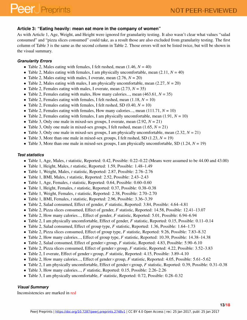
Article 3: “Eating heavily: mean eat more in the company of women”As with Article 1, Age, Weight, and Height were ignored for granularity testing. It also wasn’t clear what values “saladconsumed” and “pizza slices consumed” could take, as a result those are also excluded from granularity testing. The firstcolumn of Table 3 is the same as the second column in Table 2. Those errors will not be listed twice, but will be shown inthe visual summary.
Granularity Errors• Table 2, Males eating with females, I felt rushed, mean (1.46, N = 40)• Table 2, Males eating with females, I am physically uncomfortable, mean (2.11, N = 40)• Table 2, Males eating with males, I overate, mean (2.76, N = 20)• Table 2, Males eating with males, I am physically uncomfortable, mean (2.27, N = 20)• Table 2, Females eating with males, I overate, mean (2.73, N = 35)• Table 2, Females eating with males, How many calories..., mean (463.61, N = 35)• Table 2, Females eating with females, I felt rushed, mean (1.18, N = 10)• Table 2, Females eating with females, I felt rushed, SD (0.40, N = 10)• Table 2, Females eating with females, How many calories..., mean (111.71, N = 10)• Table 2, Females eating with females, I am physically uncomfortable, mean (1.91, N = 10)• Table 3, Only one male in mixed-sex groups, I overate, mean (2.92, N = 21)• Table 3, Only one male in mixed-sex groups, I felt rushed, mean (1.65, N = 21)• Table 3, Only one male in mixed-sex groups, I am physically uncomfortable, mean (2.32, N = 21)• Table 3, More than one male in mixed-sex groups, I felt rushed, SD (1.23, N = 19)• Table 3, More than one male in mixed-sex groups, I am physically uncomfortable, SD (1.24, N = 19)
Test statistics• Table 1, Age, Males, t statistic, Reported: 0.42, Possible: 0.22–0.22 (Means were assumed to be 44.00 and 43.00)• Table 1, Height, Males, t statistic, Reported: 1.59, Possible: 1.48–1.49• Table 1, Weight, Males, t statistic, Reported: 2.87, Possible: 2.76–2.76• Table 1, BMI, Males, t statistic, Reported: 2.52, Possible: 2.43–2.43• Table 1, Age, Females, t statistic, Reported: 0.64, Possible: 0.60–0.60• Table 1, Height, Females, t statistic, Reported: 0.37, Possible: 0.38–0.38• Table 1, Weight, Females, t statistic, Reported: 2.38, Possible: 2.70–2.70• Table 1, BMI, Females, t statistic, Reported: 2.96, Possible: 3.36–3.39• Table 2, Salad consumed, Effect of gender, F statistic, Reported: 3.84, Possible: 4.64–4.81• Table 2, Pizza slices consumed, Effect of gender, F statistic, Reported: 14.58, Possible: 12.41–13.07• Table 2, How many calories..., Effect of gender, F statistic, Reported: 5.01, Possible: 6.94–6.94• Table 2, I am physically uncomfortable, Effect of gender, F statistic, Reported: 0.15, Possible: 0.11–0.14• Table 2, Salad consumed, Effect of group type, F statistic, Reported: 1.36, Possible: 1.64–1.73• Table 2, Pizza slices consumed, Effect of group type, F statistic, Reported: 9.26, Possible: 7.83–8.32• Table 2, How many calories..., Effect of group type, F statistic, Reported: 10.39, Possible: 14.38–14.38• Table 2, Salad consumed, Effect of gender×group, F statistic, Reported: 4.83, Possible: 5.90–6.10• Table 2, Pizza slices consumed, Effect of gender×group, F statistic, Reported: 4.22, Possible: 3.52–3.83• Table 2, I overate, Effect of gender×group, F statistic, Reported: 4.15, Possible: 3.89–4.10• Table 2, How many calories..., Effect of gender×group, F statistic, Reported: 4.05, Possible: 5.61–5.62• Table 2, I am physically uncomfortable, Effect of gender×group, F statistic, Reported: 0.39, Possible: 0.31–0.38• Table 3, How many calories..., F statistic, Reported: 0.15, Possible: 2.26–2.26• Table 3, I am physically uncomfortable, F statistic, Reported: 0.72, Possible: 0.28–0.32
Visual SummaryInconsistencies are marked in red
13/18
PeerJ Preprints | https://doi.org/10.7287/peerj.preprints.2748v1 | CC BY 4.0 Open Access | rec: 25 Jan 2017, publ: 25 Jan 2017
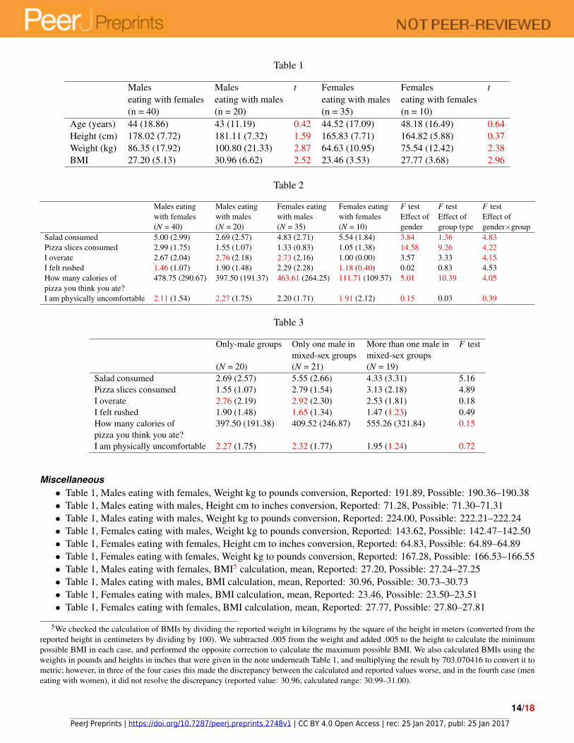
Table 1
Males Males t Females Females teating with females eating with males eating with males eating with females(n = 40) (n = 20) (n = 35) (n = 10)
Age (years) 44 (18.86) 43 (11.19) 0.42 44.52 (17.09) 48.18 (16.49) 0.64Height (cm) 178.02 (7.72) 181.11 (7.32) 1.59 165.83 (7.71) 164.82 (5.88) 0.37Weight (kg) 86.35 (17.92) 100.80 (21.33) 2.87 64.63 (10.95) 75.54 (12.42) 2.38BMI 27.20 (5.13) 30.96 (6.62) 2.52 23.46 (3.53) 27.77 (3.68) 2.96
Table 2
Males eating Males eating Females eating Females eating F test F test F testwith females with males with males with females Effect of Effect of Effect of(N = 40) (N = 20) (N = 35) (N = 10) gender group type gender×group
Salad consumed 5.00 (2.99) 2.69 (2.57) 4.83 (2.71) 5.54 (1.84) 3.84 1.36 4.83Pizza slices consumed 2.99 (1.75) 1.55 (1.07) 1.33 (0.83) 1.05 (1.38) 14.58 9.26 4.22I overate 2.67 (2.04) 2.76 (2.18) 2.73 (2.16) 1.00 (0.00) 3.57 3.33 4.15I felt rushed 1.46 (1.07) 1.90 (1.48) 2.29 (2.28) 1.18 (0.40) 0.02 0.83 4.53How many calories of 478.75 (290.67) 397.50 (191.37) 463.61 (264.25) 111.71 (109.57) 5.01 10.39 4.05pizza you think you ate?I am physically uncomfortable 2.11 (1.54) 2.27 (1.75) 2.20 (1.71) 1.91 (2.12) 0.15 0.03 0.39
Table 3
Only-male groups Only one male in More than one male in F testmixed-sex groups mixed-sex groups
(N = 20) (N = 21) (N = 19)Salad consumed 2.69 (2.57) 5.55 (2.66) 4.33 (3.31) 5.16Pizza slices consumed 1.55 (1.07) 2.79 (1.54) 3.13 (2.18) 4.89I overate 2.76 (2.19) 2.92 (2.30) 2.53 (1.81) 0.18I felt rushed 1.90 (1.48) 1.65 (1.34) 1.47 (1.23) 0.49How many calories of 397.50 (191.38) 409.52 (246.87) 555.26 (321.84) 0.15pizza you think you ate?I am physically uncomfortable 2.27 (1.75) 2.32 (1.77) 1.95 (1.24) 0.72
Miscellaneous• Table 1, Males eating with females, Weight kg to pounds conversion, Reported: 191.89, Possible: 190.36–190.38• Table 1, Males eating with males, Height cm to inches conversion, Reported: 71.28, Possible: 71.30–71.31• Table 1, Males eating with males, Weight kg to pounds conversion, Reported: 224.00, Possible: 222.21–222.24• Table 1, Females eating with males, Weight kg to pounds conversion, Reported: 143.62, Possible: 142.47–142.50• Table 1, Females eating with females, Height cm to inches conversion, Reported: 64.83, Possible: 64.89–64.89• Table 1, Females eating with females, Weight kg to pounds conversion, Reported: 167.28, Possible: 166.53–166.55• Table 1, Males eating with females, BMI5 calculation, mean, Reported: 27.20, Possible: 27.24–27.25• Table 1, Males eating with males, BMI calculation, mean, Reported: 30.96, Possible: 30.73–30.73• Table 1, Females eating with males, BMI calculation, mean, Reported: 23.46, Possible: 23.50–23.51• Table 1, Females eating with females, BMI calculation, mean, Reported: 27.77, Possible: 27.80–27.81
5We checked the calculation of BMIs by dividing the reported weight in kilograms by the square of the height in meters (converted from thereported height in centimeters by dividing by 100). We subtracted .005 from the weight and added .005 to the height to calculate the minimumpossible BMI in each case, and performed the opposite correction to calculate the maximum possible BMI. We also calculated BMIs using theweights in pounds and heights in inches that were given in the note underneath Table 1, and multiplying the result by 703.070416 to convert it tometric; however, in three of the four cases this made the discrepancy between the calculated and reported values worse, and in the fourth case (meneating with women), it did not resolve the discrepancy (reported value: 30.96; calculated range: 30.99–31.00).
14/18
PeerJ Preprints | https://doi.org/10.7287/peerj.preprints.2748v1 | CC BY 4.0 Open Access | rec: 25 Jan 2017, publ: 25 Jan 2017
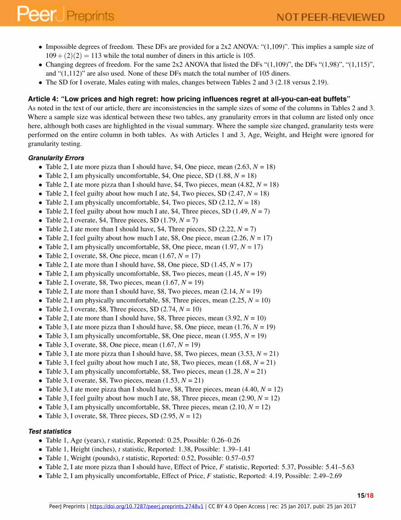
• Impossible degrees of freedom. These DFs are provided for a 2x2 ANOVA: “(1,109)”. This implies a sample size of109+(2)(2) = 113 while the total number of diners in this article is 105.
• Changing degrees of freedom. For the same 2x2 ANOVA that listed the DFs “(1,109)”, the DFs “(1,98)”, “(1,115)”,and “(1,112)” are also used. None of these DFs match the total number of 105 diners.
• The SD for I overate, Males eating with males, changes between Tables 2 and 3 (2.18 versus 2.19).
Article 4: “Low prices and high regret: how pricing influences regret at all-you-can-eat buffets”As noted in the text of our article, there are inconsistencies in the sample sizes of some of the columns in Tables 2 and 3.Where a sample size was identical between these two tables, any granularity errors in that column are listed only oncehere, although both cases are highlighted in the visual summary. Where the sample size changed, granularity tests wereperformed on the entire column in both tables. As with Articles 1 and 3, Age, Weight, and Height were ignored forgranularity testing.
Granularity Errors• Table 2, I ate more pizza than I should have, $4, One piece, mean (2.63, N = 18)• Table 2, I am physically uncomfortable, $4, One piece, SD (1.88, N = 18)• Table 2, I ate more pizza than I should have, $4, Two pieces, mean (4.82, N = 18)• Table 2, I feel guilty about how much I ate, $4, Two pieces, SD (2.47, N = 18)• Table 2, I am physically uncomfortable, $4, Two pieces, SD (2.12, N = 18)• Table 2, I feel guilty about how much I ate, $4, Three pieces, SD (1.49, N = 7)• Table 2, I overate, $4, Three pieces, SD (1.79, N = 7)• Table 2, I ate more than I should have, $4, Three pieces, SD (2.22, N = 7)• Table 2, I feel guilty about how much I ate, $8, One piece, mean (2.26, N = 17)• Table 2, I am physically uncomfortable, $8, One piece, mean (1.97, N = 17)• Table 2, I overate, $8, One piece, mean (1.67, N = 17)• Table 2, I ate more than I should have, $8, One piece, SD (1.45, N = 17)• Table 2, I am physically uncomfortable, $8, Two pieces, mean (1.45, N = 19)• Table 2, I overate, $8, Two pieces, mean (1.67, N = 19)• Table 2, I ate more than I should have, $8, Two pieces, mean (2.14, N = 19)• Table 2, I am physically uncomfortable, $8, Three pieces, mean (2.25, N = 10)• Table 2, I overate, $8, Three pieces, SD (2.74, N = 10)• Table 2, I ate more than I should have, $8, Three pieces, mean (3.92, N = 10)• Table 3, I ate more pizza than I should have, $8, One piece, mean (1.76, N = 19)• Table 3, I am physically uncomfortable, $8, One piece, mean (1.955, N = 19)• Table 3, I overate, $8, One piece, mean (1.67, N = 19)• Table 3, I ate more pizza than I should have, $8, Two pieces, mean (3.53, N = 21)• Table 3, I feel guilty about how much I ate, $8, Two pieces, mean (1.68, N = 21)• Table 3, I am physically uncomfortable, $8, Two pieces, mean (1.28, N = 21)• Table 3, I overate, $8, Two pieces, mean (1.53, N = 21)• Table 3, I ate more pizza than I should have, $8, Three pieces, mean (4.40, N = 12)• Table 3, I feel guilty about how much I ate, $8, Three pieces, mean (2.90, N = 12)• Table 3, I am physically uncomfortable, $8, Three pieces, mean (2.10, N = 12)• Table 3, I overate, $8, Three pieces, SD (2.95, N = 12)
Test statistics• Table 1, Age (years), t statistic, Reported: 0.25, Possible: 0.26–0.26• Table 1, Height (inches), t statistic, Reported: 1.38, Possible: 1.39–1.41• Table 1, Weight (pounds), t statistic, Reported: 0.52, Possible: 0.57–0.57• Table 2, I ate more pizza than I should have, Effect of Price, F statistic, Reported: 5.37, Possible: 5.41–5.63• Table 2, I am physically uncomfortable, Effect of Price, F statistic, Reported: 4.19, Possible: 2.49–2.69
15/18
PeerJ Preprints | https://doi.org/10.7287/peerj.preprints.2748v1 | CC BY 4.0 Open Access | rec: 25 Jan 2017, publ: 25 Jan 2017
• Table 2, I overate, Effect of Price, F statistic, Reported: 5.02, Possible: 4.61–4.86• Table 2, I ate more than I should have, Effect of Price, F statistic, Reported: 6.20, Possible: 5.04–5.28• Table 2, I ate more pizza than I should have, Effect of Pieces, F statistic, Reported: 10.77, Possible: 10.80–11.05• Table 2, I feel guilty about how much I ate, Effect of Pieces, F statistic, Reported: 1.49, Possible: 1.77–1.87• Table 2, I am physically uncomfortable, Effect of Pieces, F statistic, Reported: 0.25, Possible: 0.15–0.18• Table 2, I overate, Effect of Pieces, F statistic, Reported: 4.09, Possible: 4.99–5.16• Table 2, I ate more than I should have, Effect of Pieces, F statistic, Reported: 5.00, Possible: 5.61–5.78• Table 2, I feel guilty about how much I ate, Effect of Price×pieces, F statistic, Reported: 1.67, Possible: 1.13–1.20• Table 2, I am physically uncomfortable, Effect of Price×pieces, F statistic, Reported: 1.15, Possible: 1.21–1.30• Table 2, I overate, Effect of Price×pieces, F statistic, Reported: 2.27, Possible: 2.03–2.14• Table 3, I ate more pizza than I should have, One piece, F statistic, Reported: 1.62, Possible: 1.81–1.91• Table 3, I ate more pizza than I should have, Two pieces, F statistic, Reported: 2.47, Possible: 2.60–2.71• Table 3, I ate more pizza than I should have, Three pieces, F statistic, Reported: 1.34, Possible: 1.36–1.40• Table 3, I feel guilty about how much I ate, Two pieces, F statistic, Reported: 7.13, Possible: 7.54–7.79• Table 3, I am physically uncomfortable, Two pieces, F statistic, Reported: 8.11, Possible: 11.93–12.36• Table 3, I overate, Two pieces, F statistic, Reported: 1.63, Possible: 14.62–15.01• Table 3, I ate more than I should have, Two pieces, F statistic, Reported: 10.36, Possible: 10.97–11.27
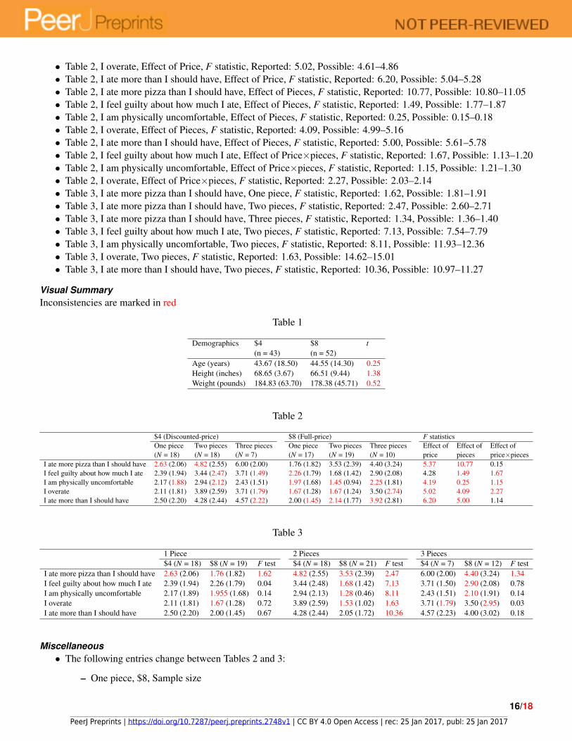
Visual SummaryInconsistencies are marked in red
Table 1
Demographics $4 $8 t(n = 43) (n = 52)
Age (years) 43.67 (18.50) 44.55 (14.30) 0.25Height (inches) 68.65 (3.67) 66.51 (9.44) 1.38Weight (pounds) 184.83 (63.70) 178.38 (45.71) 0.52
Table 2
$4 (Discounted-price) $8 (Full-price) F statisticsOne piece Two pieces Three pieces One piece Two pieces Three pieces Effect of Effect of Effect of(N = 18) (N = 18) (N = 7) (N = 17) (N = 19) (N = 10) price pieces price×pieces
I ate more pizza than I should have 2.63 (2.06) 4.82 (2.55) 6.00 (2.00) 1.76 (1.82) 3.53 (2.39) 4.40 (3.24) 5.37 10.77 0.15I feel guilty about how much I ate 2.39 (1.94) 3.44 (2.47) 3.71 (1.49) 2.26 (1.79) 1.68 (1.42) 2.90 (2.08) 4.28 1.49 1.67I am physically uncomfortable 2.17 (1.88) 2.94 (2.12) 2.43 (1.51) 1.97 (1.68) 1.45 (0.94) 2.25 (1.81) 4.19 0.25 1.15I overate 2.11 (1.81) 3.89 (2.59) 3.71 (1.79) 1.67 (1.28) 1.67 (1.24) 3.50 (2.74) 5.02 4.09 2.27I ate more than I should have 2.50 (2.20) 4.28 (2.44) 4.57 (2.22) 2.00 (1.45) 2.14 (1.77) 3.92 (2.81) 6.20 5.00 1.14
Table 3
1 Piece 2 Pieces 3 Pieces$4 (N = 18) $8 (N = 19) F test $4 (N = 18) $8 (N = 21) F test $4 (N = 7) $8 (N = 12) F test
I ate more pizza than I should have 2.63 (2.06) 1.76 (1.82) 1.62 4.82 (2.55) 3.53 (2.39) 2.47 6.00 (2.00) 4.40 (3.24) 1.34I feel guilty about how much I ate 2.39 (1.94) 2.26 (1.79) 0.04 3.44 (2.48) 1.68 (1.42) 7.13 3.71 (1.50) 2.90 (2.08) 0.78I am physically uncomfortable 2.17 (1.89) 1.955 (1.68) 0.14 2.94 (2.13) 1.28 (0.46) 8.11 2.43 (1.51) 2.10 (1.91) 0.14I overate 2.11 (1.81) 1.67 (1.28) 0.72 3.89 (2.59) 1.53 (1.02) 1.63 3.71 (1.79) 3.50 (2.95) 0.03I ate more than I should have 2.50 (2.20) 2.00 (1.45) 0.67 4.28 (2.44) 2.05 (1.72) 10.36 4.57 (2.23) 4.00 (3.02) 0.18
Miscellaneous• The following entries change between Tables 2 and 3:
– One piece, $8, Sample size
16/18
PeerJ Preprints | https://doi.org/10.7287/peerj.preprints.2748v1 | CC BY 4.0 Open Access | rec: 25 Jan 2017, publ: 25 Jan 2017

– Two pieces, $8, Sample size– Three pieces, $8, Sample size– I feel guilty about how much I ate, Two pieces, $4, SD– I feel guilty about how much I ate, Three pieces, $4, SD– I am physically uncomfortable, One piece $4, SD– I am physically uncomfortable, Two pieces $4, SD– I ate more than I should have, Three pieces, $4, SD– I am physically uncomfortable, One piece, $8, mean– I am physically uncomfortable, Two pieces, $8, mean– I am physically uncomfortable, Two pieces, $8, SD– I am physically uncomfortable, Three pieces, $8, mean– I am physically uncomfortable, Three pieces, $8, SD– I overate, Two pieces, $8, mean– I overate, Two pieces, $8, SD– I overate, Three pieces, $8, SD– I ate more than I should have, Two pieces, $8, mean– I ate more than I should have, Two pieces, $8, SD– I ate more than I should have, Three pieces, $8, mean– I ate more than I should have, Three pieces, $8, SD
• The sample sizes in Table 2 do not add up to 95• Incorrect degrees of freedom: The text describes an apparent 3x1 ANOVA with the DFs “(2, 84)”, implying a total
of 84+3 = 87 diners when there are 95 diners in total• Incorrect degrees of freedom: The text describes an apparent 2x1 ANOVA with the DFs “(1, 84)”, implying a total
of 84+2 = 86 diners when there are 95 diners in total• Table 1, Height, $8, SD seems excessively large (the SD of human height is typically around 4 inches; see also Table
1 of Article 1)• Table 1, Weight, $4, SD is large and inconsistent with the SD in the $8 condition, as well as with the SDs in Table 1
of Article 1.
ACKNOWLEDGMENTS
The authors wish to thank Chris Chambers, Pete Etchells, Eric Robinson, and James Heathers for their helpful commentson earlier drafts of this article. All errors remain the joint responsibility of the three authors.
COMPETING INTERESTS
TvdZ has a blog entitled ”The Skeptical Scientist” at timvanderzee.com. JA operates omnesres.com, oncolnc.org, andprepubmed.org. NJLB has a blog at sTeamTraen.blogspot.com that hosts advertising; his earnings in 2016 were e3.88.
AUTHOR CONTRIBUTIONS
All three authors contributed equally to this article; names are listed in ascending order of age, which we used as a surrogatefor lifetime pizza consumption.
REFERENCES
Anaya, J. (2016). The GRIMMER test: A method for testing the validity of reported measures of variability. PeerJPreprints, 4:e2400v1.
Bakker, M., van Dijk, A., and Wicherts, J. M. (2012). The rules of the game called psychological science. Perspect PsycholSci, 7(6):543–54.
17/18
PeerJ Preprints | https://doi.org/10.7287/peerj.preprints.2748v1 | CC BY 4.0 Open Access | rec: 25 Jan 2017, publ: 25 Jan 2017

Bakker, M. and Wicherts, J. M. (2011). The (mis)reporting of statistical results in psychology journals. Behavior ResearchMethods, 43(3):666–678.
BMC (2017). Bmc editorial policies. BioMed Central, https://www.biomedcentral.com/getpublished/editorial-policies.Brown, N. J. L. and Heathers, J. A. J. (2016). The GRIM test: A simple technique detects numerous anomalies in the
reporting of results in psychology. Social Psychological and Personality Science, Advance online publication:1–7.Epskamp, S. and Nuijten, M. B. (2015). Statcheck: Extract statistics from articles and recompute p values (R package
version 1.0.1).GraphPad (2017). Quickcalcs. Available at http://www.graphpad.com/quickcalcs/.Ioannidis, J. P. A. (2005). Why most published research findings are false. PLoS Medicine, 2(8):e124.John, L. K., Loewenstein, G., and Prelec, D. (2012). Measuring the prevalence of questionable research practices with
incentives for truth telling. Psychological Science, 23(5):524–532.Just, D. R., Sıgırcı, O., and Wansink, B. (2014). Lower buffet prices lead to less taste satisfaction. Journal of Sensory
Studies, 29(5):362–370.Just, D. R., Sıgırcı, O., and Wansink, B. (2015). Peak-end pizza: prices delay evaluations of quality. Journal of Product &
Brand Management, 24(7):770–778.Kirkman, B. L. and Chen, G. (2011). Maximizing your data or data slicing? Recommendations for managing multiple
submissions from the same dataset. Management and Organization Review, 7(3):433–446.Kniffin, K. M., Sıgırcı, O., and Wansink, B. (2016). Eating heavily: Men eat more in the company of women. Evolutionary
Psychological Science, 2(1):38–46.Nuijten, M. B., Hartgerink, C. H. J., Assen, M. A. L. M., Epskamp, S., and Wicherts, J. M. (2015). The prevalence of
statistical reporting errors in psychology (1985–2013). Behavior research methods, pages 1–22.Open Science Collaboration (2015). Estimating the reproducibility of psychological science. Science, 349(6251):aac4716.R Core Team (2016). R: A Language and Environment for Statistical Computing. R Foundation for Statistical Computing,
Vienna, Austria.Schwarz, N. and Clore, G. L. (2016). Evaluating psychological research requires more than attention to the n: A comment
on simonsohn’s (2015) “small telescopes”. Psychological Science, 27(10):1407–1409.Smaldino, P. E. and McElreath, R. (2016). The natural selection of bad science. R Soc Open Sci, 3(9):160384.Stangroom, J. (2017). Social science statistics. Available at http://www.socscistatistics.com/tests.StatTrek.com (2017). Stattrek. Available at http://www.stattrek.com.Sıgırcı, O. and Wansink, B. (2015). Low prices and high regret: How pricing influences regret at all-you-can-eat buffets.
BMC Nutrition, 1(1):36.Wansink, B. (2016). The grad student who never said ”no”. Healthier & Happier, http://www.brianwansink.com/
phd-types-only.
18/18
PeerJ Preprints | https://doi.org/10.7287/peerj.preprints.2748v1 | CC BY 4.0 Open Access | rec: 25 Jan 2017, publ: 25 Jan 2017