Statistical Guide to Data Analysis of Avian Monitoring ... · Statistical Guide to Data Analysis of...

Statistical Guide to Data Analysis of AvianMonitoring ProgramsBiological Technical PublicationBTP-R6001-1999

U.S. Fish & Wildlife Service

Statistical Guide to Data Analysis of AvianMonitoring ProgramsBiological Technical PublicationBTP-R6001-1999

Nadav NurPoint Reyes Bird Observatory, Stinson Beach, CA 94970

Stephanie L. JonesU.S. Fish & Wildlife Service, Mountain-Prairie Region, Denver, CO 80225

Geoffrey R. GeupelPoint Reyes Bird Observatory, Stinson Beach, CA 94970

U.S. Fish & Wildlife Service

AuthorsNadav NurPoint Reyes Bird Observatory4990 Shoreline Hwy.Stinson Beach, CA 94970-9701415/868 1221email: [email protected]

Stephanie L. JonesNongame Migratory Bird CoordinatorU.S. Fish & Wildlife Service, Mountain-Prairie RegionP.O. Box 25486 DFCDenver, CO 80225303/236 8145 ext. 608email: [email protected]

Geoff GeupelPoint Reyes Bird Observatory4990 Shoreline Hwy.Stinson Beach, CA 94970-9701415/868 1221email: [email protected]

Suggested citationNur, N., S.L. Jones, and G.R. Geupel. 1999. A statisticalguide to data analysis of avian monitoring programs.U.S. Department of the Interior, Fish and WildlifeService, BTP-R6001-1999, Washington, D.C.

ii

Preface . . . . . . . . . . . . . . . . . . . . . . . . . . . . . . . . . . . . . . . . . . . . . . . . . . . . . . . . . . . . . . . . . . . . . . . . . . . . . . . . . . . . . . . v

Chapter I. Introduction . . . . . . . . . . . . . . . . . . . . . . . . . . . . . . . . . . . . . . . . . . . . . . . . . . . . . . . . . . . . . . . . . . . . . . . . . . 1

Computer Programs . . . . . . . . . . . . . . . . . . . . . . . . . . . . . . . . . . . . . . . . . . . . . . . . . . . . . . . . . . . . . . . . . . . . . . . . . . . 1

Recommended Monitoring Methods . . . . . . . . . . . . . . . . . . . . . . . . . . . . . . . . . . . . . . . . . . . . . . . . . . . . . . . . . . . . . . 1

Methods . . . . . . . . . . . . . . . . . . . . . . . . . . . . . . . . . . . . . . . . . . . . . . . . . . . . . . . . . . . . . . . . . . . . . . . . . . . . . . . . . . . . . . 1

Methods for Assessing Abundance . . . . . . . . . . . . . . . . . . . . . . . . . . . . . . . . . . . . . . . . . . . . . . . . . . . . . . . . . . . . . . . 3

Demographic Methods . . . . . . . . . . . . . . . . . . . . . . . . . . . . . . . . . . . . . . . . . . . . . . . . . . . . . . . . . . . . . . . . . . . . . . . . . 3

Statistical Terminology and Principles . . . . . . . . . . . . . . . . . . . . . . . . . . . . . . . . . . . . . . . . . . . . . . . . . . . . . . . . . . . . 3

General Considerations of Study Design . . . . . . . . . . . . . . . . . . . . . . . . . . . . . . . . . . . . . . . . . . . . . . . . . . . . . . . . . . 4

Analysis of Vegetation and Habitat Characteristics . . . . . . . . . . . . . . . . . . . . . . . . . . . . . . . . . . . . . . . . . . . . . . . . . 6

Chapter II. Assessment of Abundance and Species Composition Using Point Counts . . . . . . . . . . . . . . . . . . . . . . 8

Analysis . . . . . . . . . . . . . . . . . . . . . . . . . . . . . . . . . . . . . . . . . . . . . . . . . . . . . . . . . . . . . . . . . . . . . . . . . . . . . . . . . . . . . . 8

Community Similarity Indexes . . . . . . . . . . . . . . . . . . . . . . . . . . . . . . . . . . . . . . . . . . . . . . . . . . . . . . . . . . . . . . . . . 11

Linear Regression . . . . . . . . . . . . . . . . . . . . . . . . . . . . . . . . . . . . . . . . . . . . . . . . . . . . . . . . . . . . . . . . . . . . . . . . . . . . 11

Analyzing Vegetation Data in Relation to Point Count Data . . . . . . . . . . . . . . . . . . . . . . . . . . . . . . . . . . . . . . . . . 19

Design . . . . . . . . . . . . . . . . . . . . . . . . . . . . . . . . . . . . . . . . . . . . . . . . . . . . . . . . . . . . . . . . . . . . . . . . . . . . . . . . . . . . . . 19

Power and Sample Size Analysis Using TRENDS . . . . . . . . . . . . . . . . . . . . . . . . . . . . . . . . . . . . . . . . . . . . . . . . . 21

Using MONITOR. . . . . . . . . . . . . . . . . . . . . . . . . . . . . . . . . . . . . . . . . . . . . . . . . . . . . . . . . . . . . . . . . . . . . . . . . . . . . 23

Power and Sample-Size Analyses: Other Sources . . . . . . . . . . . . . . . . . . . . . . . . . . . . . . . . . . . . . . . . . . . . . . . . . . 24

Chapter III. Demographic Monitoring: Mist-nets . . . . . . . . . . . . . . . . . . . . . . . . . . . . . . . . . . . . . . . . . . . . . . . . . . . . 25

Analysis of Productivity . . . . . . . . . . . . . . . . . . . . . . . . . . . . . . . . . . . . . . . . . . . . . . . . . . . . . . . . . . . . . . . . . . . . . . . 25

Analysis of Adult Survival. . . . . . . . . . . . . . . . . . . . . . . . . . . . . . . . . . . . . . . . . . . . . . . . . . . . . . . . . . . . . . . . . . . . . . 27

Design . . . . . . . . . . . . . . . . . . . . . . . . . . . . . . . . . . . . . . . . . . . . . . . . . . . . . . . . . . . . . . . . . . . . . . . . . . . . . . . . . . . . . . 30

Chapter IV. Demographic Monitoring: Nest-monitoring . . . . . . . . . . . . . . . . . . . . . . . . . . . . . . . . . . . . . . . . . . . . . . 32

Background. . . . . . . . . . . . . . . . . . . . . . . . . . . . . . . . . . . . . . . . . . . . . . . . . . . . . . . . . . . . . . . . . . . . . . . . . . . . . . . . . . 32

Analysis . . . . . . . . . . . . . . . . . . . . . . . . . . . . . . . . . . . . . . . . . . . . . . . . . . . . . . . . . . . . . . . . . . . . . . . . . . . . . . . . . . . . . 32

Additional Considerations. . . . . . . . . . . . . . . . . . . . . . . . . . . . . . . . . . . . . . . . . . . . . . . . . . . . . . . . . . . . . . . . . . . . . . 34

Alternatives to the Mayfield Method: Systematic Searching and Time-to-Failure Analysis . . . . . . . . . . . . . . 34

Vegetation Analysis in Relation to Nest-monitoring. . . . . . . . . . . . . . . . . . . . . . . . . . . . . . . . . . . . . . . . . . . . . . . . 34

Design . . . . . . . . . . . . . . . . . . . . . . . . . . . . . . . . . . . . . . . . . . . . . . . . . . . . . . . . . . . . . . . . . . . . . . . . . . . . . . . . . . . . . . 35

Chapter V. Logistic Regression . . . . . . . . . . . . . . . . . . . . . . . . . . . . . . . . . . . . . . . . . . . . . . . . . . . . . . . . . . . . . . . . . . 37

Chapter VI. Concluding Remarks . . . . . . . . . . . . . . . . . . . . . . . . . . . . . . . . . . . . . . . . . . . . . . . . . . . . . . . . . . . . . . . . . 41

References . . . . . . . . . . . . . . . . . . . . . . . . . . . . . . . . . . . . . . . . . . . . . . . . . . . . . . . . . . . . . . . . . . . . . . . . . . . . . . . . . . . 42

iii

Table of Contents

iv

Tables

1. Monitoring methods used in landbird population monitoring and their characteristics. . . . . . . . . . . . . . . . . 2

2. Potential objectives of a monitoring program and typical number of years needed for a method to achieve results. . . . . . . . . . . . . . . . . . . . . . . . . . . . . . . . . . . . . . . . . . . . . . . . . . . . . . . . . . . . . . . . . . . . . . . . . . . . . . 2

3. Example of data from point count observations conducted at three point count stations, three times during the breeding season. . . . . . . . . . . . . . . . . . . . . . . . . . . . . . . . . . . . . . . . . . . . . . . . . . . . . . . . . . . . . . . . . . . . . 10

4. Calculation of diversity, similarity and evenness indices using total bird detections across sites in burned and unburned aspen (Populus tremuloides) stands in Wyoming (from Dieni 1996). . . . . . . . . . . . . . 12

5. Linear regression analysis of number of Black-headed Grosbeaks during the breeding season. . . . . . . . . 14

6. Sample output for linear regression analyses using STATA. . . . . . . . . . . . . . . . . . . . . . . . . . . . . . . . . . . . . . . 18

7. Analysis of point count data on Sacramento River: relationship of bird species richness to Damage Index, controlling for vegetation/habitat characteristics. . . . . . . . . . . . . . . . . . . . . . . . . . . . . . . . . . . . 20

8. Analysis of mist-net captures, Sacramento River 1993: relationship to Damage Index for the six species with adequate sample size. . . . . . . . . . . . . . . . . . . . . . . . . . . . . . . . . . . . . . . . . . . . . . . . . . . . . . . . . . . . 26

9. Analysis of mist-net captures, Sacramento River, 1993: relationship of HY, and proportion HY birds caught in relation to Vegetation Damage Index. . . . . . . . . . . . . . . . . . . . . . . . . . . . . . . . . . . . . . . . . . . . . . . . . . . 26

10. Evaluation and summary of available computer program software used for the analysis of animal marking and surveying studies. . . . . . . . . . . . . . . . . . . . . . . . . . . . . . . . . . . . . . . . . . . . . . . . . . . . . . . . . . . . . . . . . 28

11. Results of SURGE analysis of Wrentits, by territory status. . . . . . . . . . . . . . . . . . . . . . . . . . . . . . . . . . . . . . 29

12. Summary of models in JOLLY and JOLLYAGE (Pollack et al. 1990). . . . . . . . . . . . . . . . . . . . . . . . . . . . . . 30

13. Power analysis for detecting differences in survivorship between two groups. . . . . . . . . . . . . . . . . . . . . . . 36

14. Logistic regression analyses of Grasshopper Sparrow presence/absence in relation to habitat features (from Holmes and Geupel 1998). . . . . . . . . . . . . . . . . . . . . . . . . . . . . . . . . . . . . . . . . . . . . . . . . . . . . . . . . 39

Figures

1A. Trend, log-linear, P = 0.001, Black-headed Grosbeak, Palomarin 1980-1992. . . . . . . . . . . . . . . . . . . . . . . . 13

1B. Trend, linear-no transformation, P = 0.004, Black-headed Grosbeak, Palomarin 1980-1992. . . . . . . . . . . 13

2A. Normal probability plot, residuals of log-transformed data, Black-headed Grosbeak. . . . . . . . . . . . . . . . 16

2B. Normal probability plot, residuals of untransformed data, Black-headed Grosbeak. . . . . . . . . . . . . . . . . 16

3. Bird species richness in relation to Vegetation Damage Index. . . . . . . . . . . . . . . . . . . . . . . . . . . . . . . . . . . . . 17

4A. Distribution of residuals: species richness vs. Vegetation Damage Index. . . . . . . . . . . . . . . . . . . . . . . . . . 19

4B. Quantile-quantile plot of residuals of species richness vs. Vegetation Damage Index against normal distribution. . . . . . . . . . . . . . . . . . . . . . . . . . . . . . . . . . . . . . . . . . . . . . . . . . . . . . . . . . . . . . . . . . . . . . . . . . . 19

5. Probability of detecting Grasshopper Sparrows in relation to Index of Perennial Grass Cover. . . . . . . . . 40

List of Tables and Figures

vv

This Statistical Guide is intended to aid fieldbiologists wishing to analyze data gathered instandardized monitoring programs for landbirds. Itgrew out of the needs expressed by the WesternWorking Group of Partners in Flight, and we thankthe members of that group for providing theincentive to develop this document. It is notintended to replace good statistical texts, but tosupplement them. We encourage readers, andespecially users, of this Guide to forward theircomments, corrections, and other advice to thesenior author for incorporation into future versionsof this Guide.

This work has been a contract between Point ReyesBird Observatory and the U.S. Fish & WildlifeService. This is PRBO Contribution 679.

References to commercial products does not implyendorsement.

AcknowledgmentsWe thank John R. Sauer, J. Scott Dieni, Ken Gerow,Daniel R. Petit, and Jon Bart for multiple reviews ofearlier drafts; John Cornely, Barry Noon, KathiePurcell, C.J. Ralph, Len Thomas, and Jerry Verneralso provided helpful discussion and comments on anearlier draft of this document. The authors, not theabove named reviewers, should be held responsiblefor any errors or outlandish opinions expressedhere. We thank Jim Nichols for providing a helpfulpreprint. We thank the USFWS NongameCoordinators: Tara Zimmerman, Bill Howe, SteveLewis, Diane Pence, Richard Coon, Kent Wohl,together with Dan Petit and John Trapp, for supportand encouragement. Special thanks to all the fieldbiologists who took the time to assist us in doing thisdocument and are out there doing the work, facingthe challenges, and balancing the issues: AdriannaAraya, Grant Ballard, Sharon Browder, MikeBryant, Claire Caldes, Lynn Clark, Paula Gouse,Ron Garcia, Todd Grant, Bill Haglan, JeanneHammond, Laura Hubers, Craig Hultberg, BethMadden, Steve Martin, Bob Murphy, Lark Osborne,Fritz Prellwitz, Pam Rizor, Vickie Roy, Kelli Stone,Julian Wood, Kodiak and McDougall Jones andmany more.

Preface

This Guide is intended to provide guidance to fieldbiologists wishing to analyze data collected onterrestrial bird populations, as part of an avianpopulation monitoring program. A second objectiveis to provide information that will help biologistsdesign such programs. The audience is similar tothat for the Handbook of Field Methods (Ralph etal. 1993), the Monitoring Bird Populations by PointCounts (Ralph et al. 1995), and in many ways thisStatistical Guide to Data Analysis of AvianMonitoring Programs can be a useful complementto the field methods handbook. At the same time,we feel this Statistical Guide can be of use to fieldbiologists studying other organisms besidesterrestrial birds. In our view, all field biologistswill benefit from taking the equivalent of 2 or 3semester courses in statistics and we assume thatreaders of this guide have completed at least thisbasic level in statistics.

This document is not intended to fill deficiencies inbasic knowledge of statistics, nor is it a substitutefor a good statistical text. Rather, this Guide isintended as a supplement to these texts. Our aim isto provide practical advice in the design and analysisof field ecological data and to provide timelyinformation about current statistical computerprograms. Two good statistical texts are provided byNeter et al. (1990) and Kleinbaum et al. (1988). Bothof these texts are “intermediate” in level; that is,they assume the reader has had a basic,introductory course in statistics. Other texts bySnedecor & Cochran (1989), Sokal & Rohlf (1995)and Zar (1996) all provide a good, general statisticalbackground. Intermediate level guides forpracticing ecologists are provided by Crawley (1993),Bart and Notz (1996) and Bart et al. (1998).Noteworthy specialized statistical ecological textsinclude Ludwig & Reynolds (1988), Skalski &Robson (1992), and Draper & Smith (1981). The lasttwo mentioned have many biological examples. Alsosee the informative review by Lancia et al. (1996).

Computer ProgramsComputer programs for summarizing and analyzingdata with general statistical packages are available,for many different levels, prices and targetaudiences. Ellison (1992) reviewed a number of

general statistical packages, but that review issomewhat out of date. One versatile statistical andgraphical package, available for DOS, Windows,and UNIX platforms, is Stata (StataCorp. 1999)(obtained from Stata Corporation, 702 UniversityDrive East, College Station, TX 77840). Specializedcomputer software programs have been created toassist with analysis of capture/recapture data (usedfor analyses of survivorship, also population size);these are reviewed and summarized in this andadditional specialized computer programs arementioned in the respective sections of this Guide.

Recommended Monitoring MethodsA wide range of methods have been used to conductavian monitoring, each tailored to meet a differentset of objectives in the face of different constraints.This Guide does not address all methods that areavailable, especially those that are more widely usedfor research or inventory. Below is a short review ofmonitoring methods available, based on Butcher(1992) and Ralph et al. (1993). The reader is referredto these references (and others cited below) foradditional information. Table 1 describes thevariables measured and subjectively assesses therelative strengths and weaknesses of each method.“Strength” and “weakness” is assessed relative tothe quality of the data gathered to meet theobjective and we have not attempted to factor in costper datum. Table 2 provides a list of monitoringobjectives, monitoring methods and the typical timerequired by the various methods to achieve thoseobjectives (from Geupel & Warkentin 1995).Descriptions of monitoring methods, theirapplications and comparisons, and their limitationscan be found in Ralph and Scott (1981), Verner(1985), Butcher (1992), Ralph et al. (1993), Bucklandet al. (1993) and Geupel & Warkentin (1995).

MethodsArea search—A method in which observers areallowed to roam for a fixed time in a specified area,usually 20 minutes per 3 hectare area (Loyn 1986,Slater 1994). This technique has a wide appeal tovolunteers but standardization of data collection isdifficult.

1

I. Introduction

2 Statistical Guide to Data Analysis of Avian Monitoring Programs

Table 1. Monitoring methods used in landbird population monitoring and their characteristics. Methods are grouped under “survey” and “demographic.” Positive or high level is denoted by “+”, negative or low level denoted by “–” and partial level denoted by “+/–“. Modified from Table 1 in Butcher(1992). “Color banding” is assumed to include nest-searching. “Rare” species refers to species that arelocally (not just globally) rare.

Survey Demographic

Fixed Spot Area Variable Mist Nest Color Variables Measured distance map Search distance net Search banding

Index to abundance + + + + +/– +/– +Density – + – + – – +Survivorship (adult) – – – – + – ++Productivity – – – – + + +Recruitment – – – – + – +Habitat Relations + + + + +/– + +/–Nest Site Characteristics – – – – – + +Predation/Parasitism – – – – – + +Individuals Identified – – – – + – +Breeding Status Known – + – – +/– + +

General Characteristics

Habitat specificity + + + + +/– + +Rare species measured + +/– + +/– – +/– +/–Canopy species measured + + + + – +/– –Area sampled known + + + + +/– + +Large area sampled + – + + +/– – –Use in non-breeding season + +/– + + + – +

Table 2. Potential objectives of a monitoring program and typical number of years needed for a method toachieve results. Actual number of years depends on study design and will vary depending on sample size (e.g., number ofcensus stations, detection or capture rates, number of nests found). We assume that the priorities of themonitoring program reflect local or site-specific needs (adapted from Geupel & Warkentin 1995).

Method

Single Point Repeat Area Spot Mist NestObjective Countsa Pt. Countsb Searchc mapping nettingd monitoringd

Inventory, species presence/absence 1 1 1 1 1 naInventory locally rare species 2-3 1-3 1-3 1-3 1-3 naDetermine species richness 2-3 1-3 1-3 1-3 na naDetermine relative abundance 1-2 1-2 1-3 1-2 3-5 naDetermine species breeding status/seasonality na 1-3 1-3 1-3 1-3 1-3Determine population trend 6-10 5-9 10+ 5-9 6-10 naDetermine productivity na na na na 1-3 1-2Determine adult survivorship na na na 3-5e 3-5 naDetermine life history traits na na na 2-4 na 1-2Habitat association or preference 1-2 1-2 1-2 1-3 na 1-2Identify habitat features 4-6 3-5 3-5 2-4 na 1-2Determine cause of pop. change na na na na 3+ 3+

a Each point count censused one time in a season.b Each point count censused 3 or more times in a season.c Each plot censused 3 or more times in a season.d Most authors/programs recommend this method in conjunction with population surveys.e Possible if birds have been uniquely color-banded.na Not applicable or not possible.

Methods for Assessing AbundancePoint counts—Fixed radius point counts are thebasic method recommended for most monitoringstudies, and are most widely used (Hutto et al. 1986,Ralph et al. 1993, Ralph et al. 1995). These canprovide a cost-effective method of estimating therelative abundance of birds.

Line transects—Fixed-width transects can providecoverage of a greater area than point counts, butwith fewer independent data points or replicates.

Variable distance methods—Estimating distance atwhich birds are detected can be incorporated intoboth point count and line transect surveys.Standardization of distance estimation may bedifficult, as abilities to accurately estimate distancesmay vary greatly between observers.

Spot-mapping—Can provide good densityinformation and information on many aspects ofavian life history. It is expensive per data point andmay be better applied to research projects or to highpriority areas or species.

Demographic MethodsIn general, demographic monitoring methods can beused to identify proximal causes of populationdeclines and provide insight into causes of habitatassociations. They can identify population problemsprior to the detection of declines based onabundance surveys. Ultimately, these methods canbe used to identify “source” or “sink” populations.However, these methods require much effort perstation.

Constant effort mist-netting—Provides informationon productivity and survivorship of populations,but is limited by area covered (which is generallyunknown) and lack of habitat specificity. However,many species can be monitored at the same time,without expending extra effort.

Nest monitoring—Provides site-specific andhabitat-specific information on productivity andreproductive status. Available personnel usuallylimit the number of plots that can be studied, andstudying additional species normally requiresincreased effort.

Color-banding—When combined with nestmonitoring, using unique color-band combinations tofollow the fates of individuals will provide the mostcomplete and unbiased measures of demographicparameters. However, it is the most intensivemethod of all. It is not a method recommended forgeneral monitoring, but like spot-mapping, bestsuited for research projects or for high priorityareas and species.

Statistical Terminology and PrinciplesThe following is a selective review of some statisticalterms relevant to a biologist conducting amonitoring study. Our intention here is to re-acquaint the reader with terms and principles thatmay have rested dormant for many years.

Accuracy—An estimator is accurate if it producesestimates that are, on average, close to the truevalue, i.e., without bias or with a minimum of bias.Accuracy is independent of precision (below). Anestimate can be accurate but not precise, precise butnot accurate, or both accurate and precise. Thedifficulty is that often the “true” value is unknownand therefore accuracy is difficult to judge, exceptfor simulated data where an investigator knows thetrue values.

Bias—The difference between the average estimate(more precisely, the expected value of the estimate)and the true value. Bias is not the same as “error”,rather it is one kind of error, systematic error. If anestimate is as likely to be an overestimate as it is tobe an underestimate, the estimator in question isunbiased, even though there will always be errorassociated with an estimate. To minimize bias would,by definition, maximize accuracy.

Precision—Precision refers to the variability of theestimate: the smaller the variability (and thus thesmaller the standard error) of the estimate, thegreater the precision. As mentioned above, precisionis independent of accuracy. An estimate can be veryprecise, but wildly inaccurate (i.e., strongly biased).

Type I and Type II errors—Rejecting the nullhypothesis when it is correct is committing a Type Ierror. The probability of committing a Type I erroris symbolized α [alpha] and is the significance levelof a test of statistical inference. Accepting the nullhypothesis when it is incorrect is committing a TypeII error; the probability of making such an error issymbolized ß [beta].

Power—The probability of detecting a biologicaleffect, if there is one. More precisely, power is theprobability of rejecting the null hypothesis when thenull hypothesis is incorrect. Normally, the nullhypothesis is an hypothesis of no effect (i.e., nodifference). Power is equal to 1–ß. Power cannot becalculated unless one specifies the alternativehypothesis: one must specify the magnitude of theeffect or difference. A given test will have greaterpower the greater the magnitude of the effect, andconversely, the smaller the true difference betweengroups, the less the power to detect that differencefor a given sample size. Power is discussed ingreater depth in Chapter II of this Guide.

Introduction 3

Poisson distribution—Among several discretedistributions (binomial, geometric, negativebinomial), this distribution is one of the most likelyto be encountered or utilized in ecological studies(Ludwig and Reynolds 1988). Many randomprocesses, in which events occur independently ofeach other, in space or time, conform to a Poissondistribution. Suppose one set up a grid of 100 one-cmsquares (10 cm × 10 cm). The number of rain dropsfalling per square in a short interval of time is likelyto be Poisson-distributed. Suppose that in oneminute, 100 rain drops fell on the 100 squares. If thisprocess was indeed a Poisson process, then we wouldexpect that in 1 minute, on average, 37 squareswould receive 0 drops, 37 squares would receive 1drop, 18 squares would receive 2 drops, and 8squares would receive 3 or more drops. For aPoisson process, the mean of occurrences (per unittime or space, in the rain drop example = 1.0 dropsper square per minute) will equal the variance ofthose occurrences. Thus, for a Poisson-distributedvariable, only one parameter is specified.

Another useful distribution is the binomialdistribution. If N independent trials were conductedand the probability of a “hit” (representing success,failure, death, etc.) on any one trial is p, then thenumber of hits in total is binomially distributed, withmean = Np, and Variance = Np(1–p). As a result,variance is neither independent of the mean (as it isin the normal distribution) nor is it equal to themean (as it is in the Poisson distribution); moreover,variance is maximized when p = 1–p = 0.5. As papproaches 0 or 1, the variance will shrink to zero.The binomial distribution is, for example, utilized inlogistic regression (Chapter V). Note that thebinomial distribution has two parameters, N and p.When the number of trials is large and theprobability of a “hit”, p, is low, then the binomialdistribution can be approximated by the Poissondistribution.

Replicates—Replicates are independent repetitionsor measurements within the experimental design. Ifrepetitions are not independent then these “repeats”are sometimes referred to as pseudoreplicates(Hurlbert 1984, Bart et al. 1998). Suppose 100 pointcount stations in a given habitat type have beensurveyed three separate times during the breedingseason. The 300 data points obtained should not betreated as 300 replicates or samples, because birddata obtained on different days in the same seasonare not independent. Whether or not the 100 pointcount stations are independent or not is difficult tosay a priori, but if spaced far enough apart (Ralphet al. 1995 recommend spacing of at least 250 m), sothat the same individuals are not being counted atdifferent stations, the 100 point count stations can betreated as independent. Assuming independence

among adjacent point count stations, and if the 100point count stations were divided evenly among 4habitats, then there would be 25 replicates.

As far as the three repeats per point count stationare concerned, one can average the data, select therepeat with the highest score for each individualspecies, or sum the data from each of the threevisits. If one wished to compare results among thethree visits (e.g., asking whether there was aseasonal, within-year trend), one can analyze the 300observations, using “point count station” as acategorical variable to be controlled for; this is anexample of a repeated-measures design, in which“point count station” is a blocking variable.

Independence of observations—This is an importantissue in statistical analysis, and is oftenmisunderstood. To start, what is required are thatoutcomes be independent from one observation toanother, after controlling for factors or variablesthat might be influencing the outcome. Suppose thepoint count stations have been spaced 100 m aparton transects of 1 km length. An investigator mightnot feel comfortable in treating observations fromdifferent stations on the same transect as beingindependent of each other. One solution would be toclassify the transect as the unit of observation, i.e.,pooling data from all point count stations on thesame transect, and analyze data accordingly.Another solution would be to include in the analysisa “transect effect.” This would control for the factthat stations on the same transect are more likely tobe similar in outcome than are stations on differenttransects. In this way one can investigatedifferences among and within transects.

A second point is that the independence refers to theoutcome, not the independent variables or factors.Suppose one related bird species richness tovegetation. As long as bird species richness variesindependently from station to station (aftercontrolling for various factors), it would not matterthat all stations on a transect shared some of thesame vegetation characteristics. In other words,there is no requirement that vegetationcharacteristics be independent from one observationunit to another.

General Considerations of Study Design General study design considerations will apply tomost monitoring techniques and studies. Neter et al.(1990) provides a good discussion of experimentaldesign, also see Skalski & Robson (1992) andCrawley (1993); those wishing more detail canconsult specialized texts such as Hicks (1982). Ahelpful and interesting discussion of the issues andthe process for designing an avian monitoring studyon one site such as a National Wildlife Refuge is


given in Johnson (In Press). In this section, wediscuss some general points concerning design of astudy. Later when discussing each methodology inturn (point counts, mist-netting and nest-monitoring), we return to questions of design.Throughout this Guide, the use of “station” refers toone independent monitoring site, e.g., one pointcount station (if observations are deemedindependent of other stations), one line transect, onemist-netting array, one nest-monitoring plot, etc. Itis important to correctly determine the unit ofanalysis early in the study design.

Design—The first and most importantconsideration in designing a study is its objectives.Statistical inference (in particular, tests ofstatistical significance) may be of little interest, inwhich case statistical power need not be consideredin determining the sample size needed. A biologistmay instead wish to monitor a particular areamainly as a descriptive tool. If data are gathered in a standardized fashion (Ralph et al. 1993), thedata from one area can contribute to regional ornational monitoring programs, which likely havestatistical inference as an objective. In many casesthe number of stations will be limited by availableresources or by the physical areas of interest.Some field biologists will be able to establish one,or at most, a couple of demographic monitoringstations (e.g., one mist-net array or onenest-monitoring plot). In those cases placement of the station will usually be constrained by thelocation and size of the habitat of interest, by thedensity of the species of special concern, or becentered on the location of the habitat or species of interest.

Data from just a single demographic monitoringstation may be valuable for several reasons: 1. the data provide a description of temporalpatterns, which data can be combined with othersources of data, 2. the data can allow statistical testsof trends over time, given sufficient number of yearsof data collection (possibly 10 years or more for asingle station), and 3. the data can be combined withdata from other monitoring stations.

Not every monitoring program needs to havehypothesis testing as its goal from the outset. Amonitoring program may be able to collect valuabledata that can later be analyzed (by itself or as partof a larger study), and that analysis would surelyinclude hypothesis testing and tests of statisticalsignificance. But it is pointless to erect contrivedhypotheses before data collection has begun, simplyin order to justify the establishment of a monitoringprogram. After data have been collected, theinvestigator will have a much better idea of how toformulate meaningful hypotheses. This point does

not apply to experimental studies, where explicithypothesis formulation is an essential ingredient toa successful study.

Assuming statistical inference is an importantconsideration, one needs to determine whether theobjective is to determine trends through time,establish bird-habitat relationships, compare effectsof different treatments, or other possible objective.Choice of objective will influence questions of samplesize and allocation of stations (see Randomizationbelow).

Assuming that statistical inference is a goal, thequestion of necessary sample size needs to berelated to statistical power, i.e., the ability to detectan effect if there is one. Statistical power is anelusive concept in part because it is arbitrary.Calculations of sample size in the past have usedpower values ranging from 50% to 95%. Clearly, thegreater the desired power, the greater the samplesize necessary to achieve that power. Generally, thisGuide uses values of 50% and 80%. In designing astudy one would not ordinarily consider 50% powerto be adequate and we do not recommend a study bedesigned to achieve 50% power. Nevertheless 50%power presents a useful level for a posterioriinvestigations, where someone has already collectedthese data and the biologist wishes to consider thestatistical power of the data to detect effects ofinterest. Conversely, in designing a study, 80%power is a commonly used and often-recommendedbenchmark, but it is nothing more than abenchmark.

Power calculations and sample size calculationsboth rely on the presumed magnitude of the effectin question. Clearly, the greater the presumedeffect (e.g., the greater the difference betweenthe two groups), the greater the power will be todetect that effect, and, conversely, the smaller thenecessary sample size to detect an effect at aspecified power. The difficulty here is that the truedifference between groups is unknown, andfurthermore one cannot necessarily use theobserved magnitude of an effect (e.g., observeddifference between two groups) as the criterionfor judging power.

It is easy to fall into the trap of estimating power,retrospectively, using the observed magnitude of aneffect, and several general statistical packagesappear to encourage users to do so, withoutappropriate warnings (discussed in Thomas andKrebs 1997). The problem is that if a statisticallysignificant effect is found, one would not normallycalculate power retrospectively. If the investigatorlooks for an effect and finds there is one, then thereis little need to determine the probability of having

Introduction 5

found that effect. Therefore, retrospective powercalculations are usually pursued only when nosignificant effect is detected. But given that no effectwas detected (statistically), it could be because theobserved magnitude of an effect was substantial, butpower was weak, or because the observedmagnitude of an effect was small, even negligible.However, power will always be low to detect anegligible effect. It is not very informative tocalculate that, given the negligible effect observed,yes, one’s power to detect a negligible effect isnegligible. Thus, to be useful, retrospective poweranalysis requires that only effects of a prioriinterest be examined. In other words, in conductingpower analysis, the magnitude of the effect ofinterest needs to be fixed independently of the dataat hand. The biologist must decide what is themagnitude of an effect worth considering; this is abiological, not a statistical, issue that is sometimesdifficult to settle.

Randomization—Randomization is an importantpart of experimental design, owing to the work ofSir Ronald Fisher in the early 20th century.Randomization is used to combat biases that canundermine survey and experimental studies. Themost important bias concerns assignment totreatments. By randomizing assignment totreatment (e.g., grazed vs. ungrazed), extraneousdifferences among experimental units can beminimized. Even here one would likely userandomization subject to constraint. Suppose onehad five land units, each one that can be divided intofour plots. Randomly choosing treatment for the 20plots could result in an unbalanced design. Instead,one can randomly choose treatment, subject to theconstraint of 10 plots for each treatment. An evenbetter design would use land unit as a blockingvariable. Within each block (here, land unit), onerandomly assigns treatment to plots, with theconstraint that there must be two plots for eachtreatment. Of course, in many studies assignment totreatment is not always under the investigator’scontrol.

Randomization should also be applied to minimizeother types of bias, if feasible. If two treatmentsare being compared using point counts, using twoobservers, one should not assign one observer toconduct point counts in treatment A and the otherobserver to conduct point counts in treatment B.In this case, observer identity and the effect of thetreatment would be confounded. Instead, the twotreatments should be divided between the twoobservers, as randomly or equitably as possible.Another bias concerns order of observation. Ifseveral plots are to be visited each day, one shouldnot visit the plots in the same order each time, butshould vary the order. It is not usually feasible to

visit point count stations in a random order, butone can usually randomize the starting point oneach visit.

The final source of bias concerns inclusion in a study.The sample to be studied will likely be the mostrepresentative of the population in question if it israndomly selected; however, this is often notfeasible. Nevertheless, we recommend incorporatingsome randomness into every study. For example, onecould lay out a grid of point count stations, centeredon a randomly selected starting point as suggestedby Sauer (1998). This approach can be adapted forthose setting up transects of point count stations:the starting point for a transect can be randomlyselected among a subset of possible points. Anotherapproach is to set up a grid of possible stations andthen randomly determine whether or not to includeindividual stations in the study. Hutto et al. (1996)and Hutto and Paige (1995) provide othersuggestions for randomizing point count stationsacross broad areas.

Analysis of Vegetation and Habitat CharacteristicsData on vegetation and habitat features can play animportant role in avian monitoring studies. Thesedata can be gathered at different scales and in manydifferent ways. Methods of vegetation datacollection are described in many publications,including Ralph et al. (1993), the BBIRD programprotocol (Martin et al. 1997), and Hays et al. (1981).One of the most influential vegetation assessmentprotocols developed for use with bird studies is byJames and Shugart (1970), with modifications byNoon (1981). The analyses of vegetation datacollected in conjunction with point counts andnest-monitoring are discussed in the appropriatesections.

Vegetation data can be collected and analyzed atseveral different scales. The broadest is habitatclassification and is qualitative (categorical) ratherthan quantitative. This level includes mostvegetation maps and can be used to select thevegetation types for study. The next broadest scaleis the “stand” level. This scale is commonly used toground-proof aerial photographs and, depending onmethods, to construct bird-habitat (or bird-vegetation) correlations, making use of point countand line transect data. The third scale involvesvegetation used to characterize the study area at asmaller scale than the first methods, often within aradius of 11.28 m following James and Shugart(1970). In some studies, plots are centered on nestsor other sites of bird use (“use sites”), while others(“non-use sites”) are randomly placed forcomparison within the study area. This scale allowsdata that are more quantitative in nature to becollected, compared to other scales. Examples of


studies using this scale are Knopf et al. (1988) andLarson & Bock (1986). This scale provides a goodmeans to establish bird-habitat relationships; suchdata can be gathered quickly, accurately andefficiently. The finest scale of vegetationmeasurement is around the nest, nest plant or othermicro-habitat features (Martin & Roper 1988;Martin et al. 1997).

Currently there is little agreement among biologistson the methods, and even the scale, of vegetationdata collection needed to correlate with birdabundance, habitat needs, distribution and behavior.Therefore, it is not possible at this time torecommend a single approach for analysis ofvegetation data since the data analytic approach willdepend on how the data were collected.

Introduction 7

Several techniques have been used for estimatingabundance of birds (Verner 1985, Bibby et al. 1992,Butcher 1992, Skalski & Robson 1992, Buckland etal. 1993, Greenwood 1996, Lancia et al. 1996). In thepast, two widely used and promoted methods havebeen point counts and line-transects (Ralph & Scott1981, Buckland et al. 1993). Capture/recapture datais a third method used to estimate populations(Greenwood 1996, Lancia et al. 1996). Following therecommendations of the National MonitoringWorking Group of Partners in Flight (Butcher 1992)and Ralph et al. (1993) and Ralph et al. (1995), werestrict our attention to point counts. Line-transectscan also yield valuable data regarding populationabundance and species composition; however, thedesign and analysis of transect data is beyond thescope of this Guide (Ralph & Scott 1981, Buckland etal. 1993). We assume that data will be collected usingfixed radius point counts, as described in Ralph et al.(1993), rather than unlimited distance point countsor variable distance point counts (Ralph & Scott1981).

Throughout this Guide we discuss how to analyzedata gathered in a typical monitoring program andthen discuss design of monitoring programs,especially sample size. Ideally, one should first putcareful thought into designing a monitoringprogram before data collection and analysis.However, here we discuss data analysis first in orderto give the reader a better idea of what sorts of datacan be gathered and what are some inferences thatcan be drawn from data collected in a monitoringprogram.

AnalysisPoint count data have commonly been analyzedwith respect to 1. relative abundance, 2. speciesrichness, 3. species diversity and 4. communitysimilarity. An alternative to the analysis of relativeabundance, has been 5. the analysis of speciespresence/absence (i.e., a species is scored as 1 if oneor more individuals are detected, and 0 ifotherwise). (We recommend not using the term“frequency of occurrence” to characterize suchanalyses, because of ambiguity of this terminology.)However, from the point of maximizing statisticalpower, the analysis of relative abundance (i.e.,number of individuals detected per station) is to be

preferred to an analysis of presence/absence. Thelatter discards information, leading to a loss ofstatistical power. On this point we are in agreementwith Dawson (1981),

“[E]ither frequency of occurrence or averagenumber [per station] is adequate measure forspecies which occur usually as one or none in eachcounting unit. On the other hand, frequencybecomes an increasingly insensitive measure forspecies found in larger numbers.”

Presence/absence may be very helpful as adescriptive tool. That is, it may be informative tostate that a species was present at 40% of stations inhabitat x and 60% of stations in habitat y. Anotheradvantage of presence/absence data is that someanalytic methods can be used for such data but notfor total detections. For example, logistic regressioncan be used with presence/absence, but not withtotal detections. Logistic regression is discussed inmore detail in Chapter V and an example is providedbelow of the analysis of presence/absence data.Nevertheless, more sophisticated variants onlogistic regression can use total detections (e.g,“ordered logistic regression”, StataCorp. 1999). Also,Poisson regression, an analytic method that hasmuch in common with logistic regression, cananalyze total detections (Kleinbaum et al. 1988). Asits name implies, Poisson regression assumes thatthe number of detections per station is Poisson-distributed, but some software (e.g., EGRET)includes the capability of testing this assumption(and modifying the analysis if data do not conform tothis assumption).

Relative abundance is analyzed as number ofdetections per unit area. The number of individualsare determined at each point count station and thisdatum can be entered into regression analyses oranalysis of variance (ANOVA). Results from severalpoint count stations can be averaged to produce asummary statistic (Example 1). If a point countstation is surveyed more than once per season, onecan either sum the number of detections over allpoint count surveys or calculate an average numberper point-count survey. As long as each station issurveyed the same number of times (e.g., threetimes), the two measures (average vs. sum) will

8

II. Assessment of Abundance and SpeciesComposition Using Point Counts

differ only by a constant, in this case, three. A thirdcommonly used method is to use the maximumnumber of detections over the course of the threesurveys. In analyzing relative abundance these threemethods can be expected to yield similar patterns.

The number of individuals detected at a point countstation is a function of the absolute abundance andthe probability of detecting an individual (given thatit is present). Analyses of relative abundanceassume that differences in detectability can beignored, for the purposes of the study. In contrast,variable distance methods (often referred to asdistance sampling; Buckland et al. 1993) attempt toestimate detectability. The assumption thatdifferences in detectability are unimportant shouldbe kept firmly in mind when considering surveys ofrelative abundance. Recent studies confirm thatdetectability is influenced by a number of differentfactors (Buckland et al. 1993, McShea & Rappole1997, Gutzwiller & Marcum 1997).

Absolute abundance. Point count data are often usedto determine relative abundance; however, absoluteabundance may be estimated using variable distancemethods (Buckland et al. 1993, Ramsey & Scott,1981). An important assumption of variable distancemethods is that at the center point of theobservation, all individuals are detected (i.e.,detectability = 100%). It is possible to relax thisassumption if, instead, the true absolute density canbe independently determined at the center point,but this is often not feasible. A second importantassumption is that individuals do not move towardsor away from the observer before being detected.Buckland et al. (1993) provide extensive discussion ofthese and other assumptions. The same authorshave developed a program DISTANCE that carriesout such analyses (Laake et al. 1993, Web site:<http://www.ruwpa.st-and.ac.uk/distance/>).

Species richness is analyzed as total number ofspecies detected. A total can be calculated for eachpoint count station, or for each group of point countstations (Example 1).

There are a plethora of indices for species diversity(Magurran 1988, Ludwig & Reynolds 1988). Theutility of diversity indices has been stronglyquestioned by some (Verner & Larson 1989), andtheir use has limitations. It has been argued thatspecies richness, a component of species diversity, ismore easily and more accurately measured. Speciesrichness is highly correlated with species diversityand can be interpreted more clearly (Verner &Larson 1989). An example of the value of a diversityindex (but one that is admittedly extreme) is acomparison of two communities, each containing fivespecies and each with a total of 100 individuals.

Community A contains 96 individuals of species 1and 1 individual of each of the other 4 species;community B contains 20 individuals of each of fivespecies. Which community is more diverse? If onefeels that both are equally diverse, then speciesrichness is all one needs to take into account.However, if one’s view is that community B is morediverse, because its bird community is moreheterogeneous, then one is justified in using adiversity index. However, keep in mind that moreassumptions are required to estimate diversity thanspecies richness. In particular, calculations ofspecies diversity assume that relative abundance isaccurately estimated and ignores the differences indetectability among species that can skew estimatesof relative abundance.

The most widely used diversity index is referred toas Shannon’s index, or as the Shannon-Wiener indexor the Shannon-Weaver index (Krebs 1989).Shannon’s index, which is derived from informationtheory, reflects both species richness and evennessof distribution among species present. An equationfor the Shannon index, using natural logarithms(ln) is:

where S = number of species in the sample, and piis the proportion of all individuals belonging to theith species. The original Shannon index wascalculated in terms of logarithm base 2, and thus H'was expressed in terms of bits; however, it is morecommon and more convenient to use naturallogarithms, as we have done above. A usefultransformation of H' is given by eH', which has beenlabeled N1 (MacArthur 1965).

N1 expresses diversity in terms of species instead ofbits and thus is easier to interpret. N1 provides thenumber of species that would, if each were equallycommon, yield the same H' value as the actualsample. For example, suppose there are 3 species, 20of species A, 20 of species B and 10 of species C.Using the above equation, H' = 1.055 and N1 = 2.87.These three species, in their uneven distribution,yield the same diversity value as would 2.87 speciesof equal abundance. A comparison of speciesrichness (= S = 3) with N1 (= 2.87) gives us ameasure of evenness of species distribution. That isthe species distribution is maximally even whenS = N1.

For a fixed S, the maximum diversity (Hmax) is equalto –ln (1/S) = ln(S) and therefore the ratio ofobserved diversity to maximum diversity is ameasure of evenness (E): E = H'/Hmax = H'/ln S

i=SH′ = Σ(pi)(lnp), i=1, 2,…S

i=1

Assessment of Abundance and Species Composition Using Point Counts 9

(Examples 1 and 2). If some species are moredetectable than others this will bias one’s measure ofdiversity, either upwards or downwards. If theShannon index is calculated for a number ofsamples, the indices themselves will be normallydistributed, making it possible to use parametricstatistics to compare sets of samples using diversityindices (Magurran 1988). Further techniques for theanalysis of diversity patterns are described inMagurran (1988) and Pielou (1975).

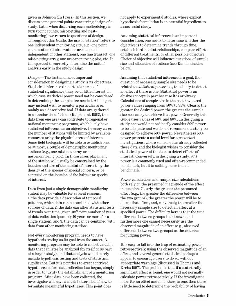
Example 1: Calculation of Summary StatisticsThe following is a simple and hypothetical exampleof data collected using point counts (Table 3).Observations were made at 3 point count stations at3 different times during the breeding season.Species are uniquely identified by a single letter(A, B, C, etc.).

From these data, summary statistics can becalculated, first of all summing (or averaging) acrossthe three survey periods, and then summing (oraveraging) across the three point count stationswhose data have already been summed over the 3survey periods. Such a summarization is shown inTable 3B.

The results shown in Table 3A for each point countstation can be used in a statistical analysis (e.g.,regression or ANOVA) (Example 3). The biologistmay also summarize results for a group of pointcount stations characterized by an importantsimilarity, e.g., all stations at a specific site, or allstations in a specific habitat on a refuge, or otherunit of interest.

The row titled “Average” in Table 3B (second fromthe bottom), simply averages the results from pointcount stations 1-3. The row titled “Cumulative”(bottom) shows the total number of individuals seenat the 3 point count stations (a measure ofabundance), the total species richness for the 3stations, and the species diversity as measured forall 3 stations taken together. Thus, the averagestation had 5 species, but the three stations togetherhad 7 different species. For average number ofindividuals seen per point count survey, the“Cumulative” value is simply three times that of the“Average” value (i.e., 12.33 = 4.11 × 3). Thus the onlydifference between these two measures is that inone case one sums the number of individuals anddivides by the number of point count stations and inthe other case one sums and does not divide. Anystatistical results will be identical whichevermeasure of individuals detected is used, except for a


Table 3. Example of data from point count observations conducted at three point count stations, three timesduring the breeding season.

A. Results by species. “A, A” indicates two individuals of species A were seen, “A, A, A” indicates three individuals, “A, B, C” indicates one individual of three species, etc.

Point Count Survey Species Number of Species Station Number Observed Individuals Richness

1 1 A, A, B, C 4 31 2 B, B, C, D 4 31 3 A, C, D, E 4 42 1 B, B, B, C 4 22 2 B, B, D 3 22 3 B, B, F 3 23 1 B, C, C, D 5 33 2 B, C, E, F, F 5 43 3 B, C, E, F, F, G 6 5

B. Summarization of data from Table 4A.

Point Count Average Number Cumulative EcologicalStation Individuals Species Richness Species Diversity1 Eveness = E

1 4.0 5 4.69 0.9602 3.33 4 2.56 0.6783 5.0 6 5.24 0.924

Average 4.11 5.0 3.86 0.839Cumulative 12.33 7 5.55 0.881

1 Shannon’s index expressed as N1

constant (in this case, 3, the number of point countstations).

In contrast to measures of abundance, Averagespecies richness and Cumulative species richness,will generally not be so simply related to each other.At one extreme average species richness will equalcumulative species richness where there is completeoverlap of species at each point count station. At theother extreme, cumulative species richness will bethree times that of average species richness(assuming one is summarizing data from three pointcount stations) provided there is no species overlapat any point count station. Reality will usually fallsomewhere in between. Either way of summarizingspecies richness can be justified. The same holds forspecies diversity; the average diversity (per pointcount station) and the diversity of the group of pointcount stations are both legitimate ways tocharacterize diversity.

Community Similarity IndexesAnother method of comparing communities is tomeasure the degree of association or similarity incommunity composition between sites or samples.For example, two sites may be identical in speciesrichness, but both have completely different species.For this purpose, a wide range of similarity indiceshave been developed (Magurran 1988). Two suchindices that are widely used and that rely only onpresence/absence data are the Jaccard index andSorensen index (Krebs 1989):

where j = the number of species found at both site Aand B, a = the number of species in site A and b =the number of species found in site B. These indicesare designed to equal 1 where the species from thetwo sites are the same and 0 if the sites have nospecies in common. Example 2 and Table 4 providean example of a calculation of Jacard and Sorensonsimilarity coefficients.

One of the advantages to these indices is theirsimplicity, but the indices do not account fordifferences in the abundance of species. All speciescount equally in the equation whether they areabundant or rare. For this reason, quantitativeindices of similarity have much appeal as analternative. Again, many such indices have beendeveloped (Magurran 1988, Krebs 1989). Here wejust mention one of the simplest, the Renkonen

2jSorenson Cs = _______

a+b

jJaccard Cj = _______

a+b–j

index, also called the Percentage Similarity index.The formula for the Renkonen index (P) is:

where pAi is the percentage of species i in sample A

and pBi is the percentage of species i in sample B

and S is the number of species found in eithersample. With no overlap between samples the indexequals 0, with complete similarity the Renkonenindex equals 100%. Table 4 provides an example ofthe Renkonen index.

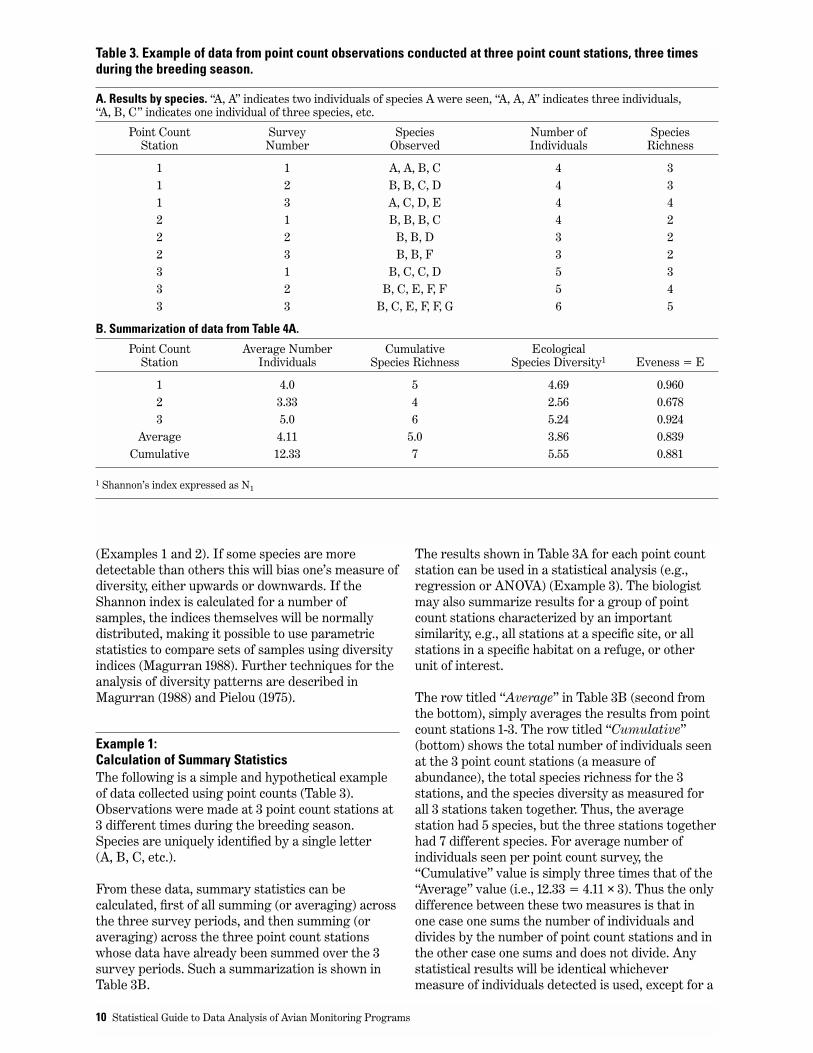
Example 2: Calculation of Community Similarity IndicesThe following is an simplified example of datacollected using point counts (Table 4). Observationswere pooled using the highest number countedduring 3 different surveys in the breeding season,and pooled across 5 paired treatment-control plots(modified from Dieni 1996). Community similarityand diversity indices can be calculated andcomparisons made using these data.

The row titled “number of individuals” in Table 4 isthe sum of the total number of individuals counted ineach site. The columns titled “pa” and “pb” are theproportion of each species in the total; i.e., thenumber of individuals divided by the total number ofindividuals for that site. The calculation of Jaccard’sindex is the number of species in common (j) to bothsites divided by the difference between the sum ofthe number of species in each site minus the numberin common. Sorenson’s index is 2 times j divided bythe summation of the number of species in bothsites.

Other indices may also be informative including theRenkonen index which is calculated by taking thesummation of the minimum of either pa or pb. Otherexamples of the calculations of indices that may beuseful are shown in Table 4.

Linear RegressionTo introduce linear regression, and provide a simpleexample of trend analysis we consider the following.

Example 3: An Example of Simple RegressionBlack-headed Grosbeaks (Pheucticusmelanocephalus) have been surveyed at thePalomarin station of Point Reyes National Seashoreduring the breeding season for many years. Here wepresent data from 1980-1992 (13 years) and wish to

i=SP = Σ minimum (pA

i , pBi)

i=1


determine if there has been a trend for numbers toincrease or decrease during this period.

Keep in mind four key assumptions of linearregression analysis:

1. Normality of residuals

2. Homoscedasticity; that is, there are no systematicdifferences in variance of residuals

3. Independence of the outcome variable (i.e.,independence of residuals), and

4. That we are interested in testing the hypothesis(HA) that there is some sort of linear relationshipbetween dependent and independent variable. In

this case, the hypothesis is that bird abundance isdecreasing or increasing with time, in a linearfashion.

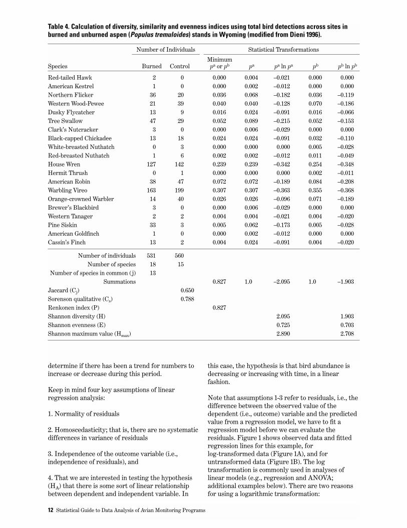
Note that assumptions 1-3 refer to residuals, i.e., thedifference between the observed value of thedependent (i.e., outcome) variable and the predictedvalue from a regression model, we have to fit aregression model before we can evaluate theresiduals. Figure 1 shows observed data and fittedregression lines for this example, forlog-transformed data (Figure 1A), and foruntransformed data (Figure 1B). The logtransformation is commonly used in analyses oflinear models (e.g., regression and ANOVA;additional examples below). There are two reasonsfor using a logarithmic transformation:


Table 4. Calculation of diversity, similarity and evenness indices using total bird detections across sites inburned and unburned aspen (Populus tremuloides) stands in Wyoming (modified from Dieni 1996).

Number of Individuals Statistical Transformations

MinimumSpecies Burned Control pa or pb pa pa ln pa pb pb ln pb

Red-tailed Hawk 2 0 0.000 0.004 –0.021 0.000 0.000American Kestrel 1 0 0.000 0.002 –0.012 0.000 0.000Northern Flicker 36 20 0.036 0.068 –0.182 0.036 –0.119Western Wood-Pewee 21 39 0.040 0.040 –0.128 0.070 –0.186Dusky Flycatcher 13 9 0.016 0.024 –0.091 0.016 –0.066Tree Swallow 47 29 0.052 0.089 –0.215 0.052 –0.153Clark’s Nutcracker 3 0 0.000 0.006 –0.029 0.000 0.000Black-capped Chickadee 13 18 0.024 0.024 –0.091 0.032 –0.110White-breasted Nuthatch 0 3 0.000 0.000 0.000 0.005 –0.028Red-breasted Nuthatch 1 6 0.002 0.002 –0.012 0.011 –0.049House Wren 127 142 0.239 0.239 –0.342 0.254 –0.348Hermit Thrush 0 1 0.000 0.000 0.000 0.002 –0.011American Robin 38 47 0.072 0.072 –0.189 0.084 –0.208Warbling Vireo 163 199 0.307 0.307 –0.363 0.355 –0.368Orange-crowned Warbler 14 40 0.026 0.026 –0.096 0.071 –0.189Brewer’s Blackbird 3 0 0.000 0.006 –0.029 0.000 0.000Western Tanager 2 2 0.004 0.004 –0.021 0.004 –0.020Pine Siskin 33 3 0.005 0.062 –0.173 0.005 –0.028American Goldfinch 1 0 0.000 0.002 –0.012 0.000 0.000Cassin’s Finch 13 2 0.004 0.024 –0.091 0.004 –0.020

Number of individuals 531 560Number of species 18 15

Number of species in common (j) 13Summations 0.827 1.0 –2.095 1.0 –1.903

Jaccard (Cj) 0.650Sorenson qualitative (Cs) 0.788Renkonen index (P) 0.827Shannon diversity (H) 2.095 1.903Shannon evenness (E) 0.725 0.703Shannon maximum value (Hmax) 2.890 2.708

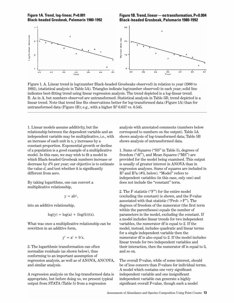
1. Linear models assume additivity, but therelationship between the dependent variable and anindependent variable may be multiplicative, i.e., withan increase of each unit in x, y increases by aconstant proportion. Exponential growth or declineof a population is a good example of a multiplicativemodel. In this case, we may wish to fit a model inwhich Black-headed Grosbeak numbers increase ordecrease by d% per year; our objective is to estimatethe value d, and test whether it is significantlydifferent from zero.

By taking logarithms, one can convert amultiplicative relationship,

y = abx,

into an additive relationship,

log(y) = log(a) + (log(b))(x).

What was once a multiplicative relationship can berewritten in an additive form,

y′ = a′ + b′x.

2. The logarithmic transformation can oftennormalize residuals (as shown below), thusconforming to an important assumption ofregression analysis, as well as of ANOVA, ANCOVA,and similar analysis.

A regression analysis on the log-transformed data isappropriate, but before doing so, we present typicaloutput from STATA (Table 5) from a regression

analysis with annotated comments (numbers belowcorrespond to numbers on the output). Table 5Ashows analysis of log-transformed data; Table 5Bshows analysis of untransformed data.

1. Sums of Squares (“SS” in Table 5), degrees offreedom (“df ”), and Mean Squares (“MS”) areprovided for the model being examined. This outputis usually of greater interest in ANOVA than inregression analyses. Sums of squares are included inR2 and R2a (#3, below). “Model” refers toindependent variables (in this case, only one) anddoes not include the “constant” term.

2. The F statistic (“F”) for the entire model(excluding the constant) is shown, and the P-valueassociated with that statistic (“Prob >F”). Thedegrees of freedom of the numerator (the first termwithin the parentheses) equals the number ofparameters in the model, excluding the constant. Ifa model includes linear trends for two independentvariables, the numerator df is equal to 2. If themodel, instead, includes quadratic and linear termsfor a single independent variable then thenumerator df is also equal to 2. If the model includeslinear trends for two independent variables andtheir interaction, then the numerator df is equal to 3,and so on.

The overall P-value, while of some interest, shouldbe of less concern than P-values for individual terms.A model which contains one very significantindependent variable and one insignificantindependent variable can generate a highlysignificant overall P-value, though such a model


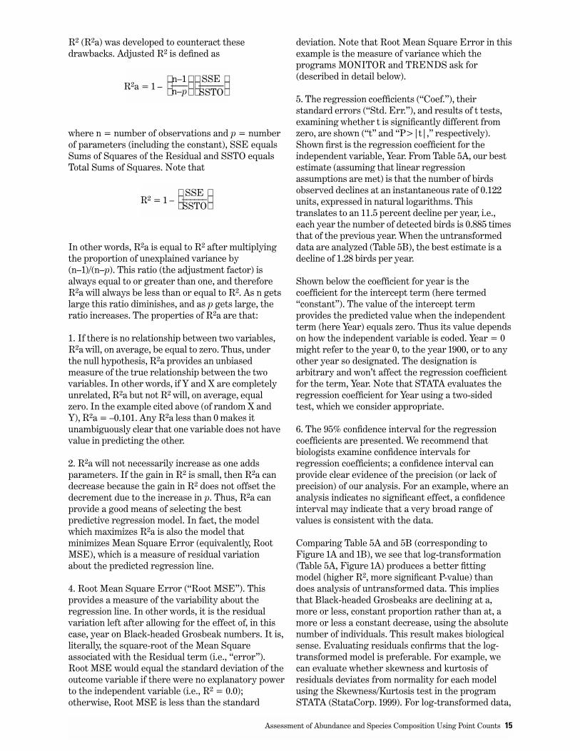
Figure 1. A. Linear trend in log(number Black-headed Grosbeaks observed) in relation to year (1980 to1992), (statistical analysis in Table 5A). Triangles indicate log(number observed) in each year; solid lineindicates best-fitting trend using linear regression analysis. The trend depicted is a log-linear trend.B. As in A. but numbers observed are untransformed. Statistical analysis in Table 5B; trend depicted is alinear trend. Note that trend line fits observations better for log-transformed data (Figure 1A) than foruntransformed data (Figure 1B); e.g., with a higher R2 0.637 vs. 0.545.

Figure 1A. Trend, log-linear, P=0.001Black-headed Grosbeak, Palomarin 1980-1992

Figure 1B. Trend, linear—no transformation, P=0.004Black-headed Grosbeak, Palomarin 1980-1992

would be undesirable. On the other hand, if twoindependent variables are highly correlated, eachvariable could be insignificant (when controlled forthe other), yet the overall model could be verysignificant and provide a good predictive model.

3. R2 (“R-square”) and adjusted R2 (“Adj R-square”).The first statistic is often referred to as thecoefficient of determination. While it should befamiliar to all field biologists, much confusion stillsurrounds its use or abuse (Anderson-Sprecher1994). The second statistic is probably unfamiliar tomany, yet should be more widely known and used(Neter et al. 1990, Kleinbaum et al. 1988). R2 can beinterpreted as the proportion of variation in thedependent variable that can be accounted for by themodel in question. Both statistics provide a measureof the predictive ability of a model. If R2 andadjusted R2 are low, this means that much variationin the Y variable is not accounted for by the model,but this does not reflect on the adequacy of the

model. In Table 5A, R2 = 0.637, meaning that 36% ofthe variation in Black-headed Grosbeak numbers isnot accounted for by an exponential decline innumbers with increasing year.

There are several drawbacks to R2. For one, anyregression model will have a positive R2 associatedwith it, even a regression model that links twovariables that are completely unrelated. To providean example, we generated two random variables X,Y, integers chosen from a uniform distribution (0,100) and which were independent of each other.Values for X were (3, 67, 98, 63, 25, 90, 34, 4, 31, 78)and for Y were (44, 91, 30, 92, 26, 56, 57, 90, 81, 47).Regressing Y on X we obtain R2 = 0.021 (P = 0.69).We would feel uncomfortable in stating that “Xaccounted for 2.1% of the variation in Y,” since inreality we know that it accounts for no suchvariation. The second drawback is that as one addsadditional terms (additional independent variables),R2 will always increase (Neter et al. 1990). Adjusted


Table 5A. Linear regression analysis of number of Black-headed Grosbeaks, breeding season, log-transformed (=ltotbrs) vs. year.

Source SS df MS Number of obs = 13

Model 2.71854704 1 2.71854704 F (1, 11) = 19.31

Residual 1.54865857 11 .140787142 Prob > F = 0.0011

Total 4.26720561 12 .355600468 Rsquare = 0.6371

Adj Rsquare = 0.6041

Root MSE = .37522

ltotbrs Coef. Std. Err. t P>|t| [95% Conf. Interval]

year .1222173 .0278129 4.394 0.001 .183433 .0610016_cons 245.1384 55.23646 4.438 0.001 123.5637 366.713

Table 5B. Linear regression analysis of number of Black-headed Grosbeaks, breeding season, untransformed (=totalbrs) vs. year.


Model 298.291209 1 298.291209 F (1, 11) = 13.20

Residual 248.631868 11 22.6028971 Prob > F = 0.0039

Total 546.923077 12 45.5769231 Rsquare = 0.5454


Root MSE = 4.7543

totalbrs Coef. Std. Err. t P>|t| [95% Conf. Interval]

year 1.28022 .3524085 3.633 0.004 2.055866 .504574_cons 2554.44 699.8845 3.650 0.004 1014.004 4094.875

①

⑤

⑥

②

③

④

R2 (R2a) was developed to counteract thesedrawbacks. Adjusted R2 is defined as

where n = number of observations and p = numberof parameters (including the constant), SSE equalsSums of Squares of the Residual and SSTO equalsTotal Sums of Squares. Note that

In other words, R2a is equal to R2 after multiplyingthe proportion of unexplained variance by(n–1)/(n–p). This ratio (the adjustment factor) isalways equal to or greater than one, and thereforeR2a will always be less than or equal to R2. As n getslarge this ratio diminishes, and as p gets large, theratio increases. The properties of R2a are that:

1. If there is no relationship between two variables,R2a will, on average, be equal to zero. Thus, underthe null hypothesis, R2a provides an unbiasedmeasure of the true relationship between the twovariables. In other words, if Y and X are completelyunrelated, R2a but not R2 will, on average, equalzero. In the example cited above (of random X andY), R2a = –0.101. Any R2a less than 0 makes itunambiguously clear that one variable does not havevalue in predicting the other.

2. R2a will not necessarily increase as one addsparameters. If the gain in R2 is small, then R2a candecrease because the gain in R2 does not offset thedecrement due to the increase in p. Thus, R2a canprovide a good means of selecting the bestpredictive regression model. In fact, the modelwhich maximizes R2a is also the model thatminimizes Mean Square Error (equivalently, RootMSE), which is a measure of residual variationabout the predicted regression line.

4. Root Mean Square Error (“Root MSE”). Thisprovides a measure of the variability about theregression line. In other words, it is the residualvariation left after allowing for the effect of, in thiscase, year on Black-headed Grosbeak numbers. It is,literally, the square-root of the Mean Squareassociated with the Residual term (i.e., “error”).Root MSE would equal the standard deviation of theoutcome variable if there were no explanatory powerto the independent variable (i.e., R2 = 0.0);otherwise, Root MSE is less than the standard

SSE ______ SSTOR2 = 1 –

SSE ______ SSTO

n–1 ____ n–pR2a = 1 –

deviation. Note that Root Mean Square Error in thisexample is the measure of variance which theprograms MONITOR and TRENDS ask for(described in detail below).

5. The regression coefficients (“Coef.”), theirstandard errors (“Std. Err.”), and results of t tests,examining whether t is significantly different fromzero, are shown (“t” and “P>|t|,” respectively).Shown first is the regression coefficient for theindependent variable, Year. From Table 5A, our bestestimate (assuming that linear regressionassumptions are met) is that the number of birdsobserved declines at an instantaneous rate of 0.122units, expressed in natural logarithms. Thistranslates to an 11.5 percent decline per year, i.e.,each year the number of detected birds is 0.885 timesthat of the previous year. When the untransformeddata are analyzed (Table 5B), the best estimate is adecline of 1.28 birds per year.

Shown below the coefficient for year is thecoefficient for the intercept term (here termed“constant”). The value of the intercept termprovides the predicted value when the independentterm (here Year) equals zero. Thus its value dependson how the independent variable is coded. Year = 0might refer to the year 0, to the year 1900, or to anyother year so designated. The designation isarbitrary and won’t affect the regression coefficientfor the term, Year. Note that STATA evaluates theregression coefficient for Year using a two-sidedtest, which we consider appropriate.

6. The 95% confidence interval for the regressioncoefficients are presented. We recommend thatbiologists examine confidence intervals forregression coefficients; a confidence interval canprovide clear evidence of the precision (or lack ofprecision) of our analysis. For an example, where ananalysis indicates no significant effect, a confidenceinterval may indicate that a very broad range ofvalues is consistent with the data.

Comparing Table 5A and 5B (corresponding toFigure 1A and 1B), we see that log-transformation(Table 5A, Figure 1A) produces a better fittingmodel (higher R2, more significant P-value) thandoes analysis of untransformed data. This impliesthat Black-headed Grosbeaks are declining at a,more or less, constant proportion rather than at, amore or less a constant decrease, using the absolutenumber of individuals. This result makes biologicalsense. Evaluating residuals confirms that the log-transformed model is preferable. For example, wecan evaluate whether skewness and kurtosis ofresiduals deviates from normality for each modelusing the Skewness/Kurtosis test in the programSTATA (StataCorp. 1999). For log-transformed data,


we cannot reject the hypothesis of normality (P =0.25), whereas for untransformed data we can rejectthe assumption of normality (P = 0.0003) (resultsobtained using “sktest” in the program STATA).

Results will not always be this clear-cut; we maywant to use graphical methods to examine normalityof residuals. Figure 2 shows a normal probabilityplot for transformed (Figure 2A) and untransformeddata (Figure 2B). We won’t go into the details ofthese plots (interested readers can refer toKleinbaum et al. 1988, Neter et al. 1990); the mainpoint is that if residuals are normally distributed,the data points will fall on the straight line shown.For the log-transformed data there is a reasonablygood match between data points and the line; foruntransformed data there is not. The graphicalmethod does not determine whether or not theresiduals are normally distributed. It does indicateto what extent transformation is or is not improvingthe normality of residuals.

Example 4: Application of Simple and Multiple RegressionWe now tackle a more complex example, taken from astudy by the Point Reyes Bird Observatory,conducted for the California Department of Fish &Game (Nur et al. 1994). We use this example as anopportunity to provide guidance in carrying outmultiple regression analysis. In July1991an herbicide

was accidentally spilled in and near the SacramentoRiver, close to Dunsmuir, CA, resulting in the death ofall aquatic forms of life for a 36-mile stretch of river.In addition, terrestrial fauna and flora along the riverwere thought to have been impacted. Nur et al. (1994)report results of an avian monitoring projectdesigned to assess the impact of the spill onterrestrial bird populations. A quantitative measureof presumed impact was developed by CaliforniaDepartment of Fish & Game biologists, relying ondefoliation, leaf death and other symptoms of stressexhibited by the riparian vegetation, which we termthe Vegetation Damage Index. Sites along the rivervaried in the degree of impact, depending on theexposure to the herbicide. In general sites closer tothe spill site in the downstream direction receivedgreater damage, and therefore higher values of thedamage index. Point counts were laid out in transectsof 7 stations per transect, stations spaced 300 mapart, with each transect parallel to the river and1800m in length, with one transect per “site”. All transectswere in riparian habitat.

In general, there was a tendency for areas with highdamage to show low species richness (Figure 3). Inparticular, there was an overall significant lineartrend for bird species richness to decline withincreasing damage, when analyzing all 55 pointcount stations. Output for this analysis is shown inTable 6A (using the program STATA). Note that inTable 6A, R2 = 0.149, meaning that 85% of thevariation in species richness among point count


Figure 2. Evaluating the assumption of normality using graphical techniques. Comparison of “Normalprobability plots” depicting residuals from analysis of log-transformed (Figure 2A) and untransformed(Figure 2B) observations of Black-headed Grosbeaks. Figure 2A and 2B depict the empirical cumulativedistribution function expected if the variable were normally distributed (y-axis) vs. the observed cumulativedistribution function (x-axis). If the variable in question were normally distributed then the graphed pointswould fall exactly on the solid line and the correlation between the two cumulative distribution functionswould be +1.0. Log-transformed data conform better to a normal distribution than do untransformedobservations.

Figure 2A. Normal probability plot, residuals of log-transformed dataBlack-headed Grosbeak

Figure 2B. Normal probability plot, residuals of untransformed dataBlack-headed Grosbeak

stations is not accounted for by differences in thedamage index. Our interpretation of this result isthat species richness data from individual pointcount stations are very variable. The model is,however, highly significant, and we have no reason tothink the model is inadequate.

One needs to keep in mind that there are twodifferent objectives for which one can use regressionmodels: (i) hypothesis testing, and (ii) prediction. Inthis case, a model with only vegetation damagewould poorly predict species richness at a specificpoint count station. However, such a model achievesthe objective of confirming the hypothesis thatbiological damage resulting from the spill wasassociated with diminished species richness.

Also keep in mind that the magnitude of R2 dependson the unit of analysis. If one were to average datafrom several point counts and then use the averageddata in a regression analysis, this would have littleeffect on the P-value, yet would increase R2

substantially. This is because some of the variationin the dependent variable has been eliminated byusing mean species richness values in the regressionanalysis, rather then species richness at individualpoint count stations.

We confirmed that the linear regression analysis inTable 6A is appropriate, first by examiningnormality of residuals: P = 0.50, using the skewness/kurtosis test (“sktest” of STATA). In other words,

residuals do not appear to deviate from normality.We demonstrate this point graphically in Figure 4.Figure 4A shows the frequency distribution ofresiduals compared to a normal distribution; Figure4B shows a quantile-normal plot for the residualsfrom Table 6A. (Quartiles and percentiles areexamples of quantiles; a quantile-normal plot showsquantiles for the distribution of interest vs. quantilesfrom a normal distribution which matches the firstdistribution in terms of mean and variance.) As witha normal-probability plot (Figure 2), if thedistribution is indeed normal, then the data points(quantiles in this case) would fall on the solid lineshown in the Figure 4B. In this case, there seems tobe a very good match, implying that residuals areapproximately, normally-distributed.

That bird species richness was correlated with theVegetation Damage Index is not by itself adequateevidence for a causal link. In a similar fashion to theanalysis in Table 6A, a suite of vegetationcharacteristics were examined, to determinewhether bird species richness, diversity andabundance were related to habitat or vegetationfeatures. If so, such habitat variables could beconfounding any relationship of the bird fauna to theimpact of the spill. In one scenario, there could be notrue functional relationship between bird speciesrichness and vegetation damage, but a correlationbetween the two can arise if both are correlated witha vegetation feature. In another scenario, the truecausal relationship between bird species richnessand vegetation damage could be strong but it couldbe masked, wholly or in part, because both arecorrelated with a vegetation feature. For example, ifbiological damage from the spill lowered speciesrichness, and the presence of willow (Salix spp.)increased species richness, then if biological damagewas greatest in an area where willows were mostabundant, the correlation between biologicaldamage and bird species richness could be veryweak despite a strong causal relationship betweenthe latter two variables.

Nur et al. (1994) examined 25 habitat features todetermine whether they might be correlated withabundance, species richness and/or species diversity.They found that only two habitat features weresignificantly correlated with abundance, speciesrichness and diversity. The latter variables werepositively correlated to the presence of willowspecies and negatively with the presence of big-leafmaple (Acer macrophyllum), i.e., the more big-leafmaple, the fewer the bird species detected. Theindependent variables were indices based on percentcover that was willow (on a 0 to 10 scale,corresponding to 0 to 100%), and percent cover ofbig-leaf maple. Results of simple linear regression ofbird species richness in relation to willow cover and


Figure 3. Bird species richness from 55 point countstations along the Sacramento River, in relation toVegetation Damage Index. Higher values implygreater damage from spill of metam sodium(statistical results in Table 6A). Least squares line ofbest fit is shown. Data at each point count stationhave been “jittered” (Stata Corp. 1997) to reduceoverlap of points.

Figure 3. Bird species richness in relation toVegetation Damage Index.

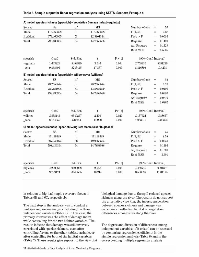
in relation to big-leaf maple cover are shown inTables 6B and 6C, respectively.

The next step in the analysis was to conduct amultiple regression analysis including the threeindependent variables (Table 7). In this case, theprimary interest was the effect of damage indexwhile controlling for the two habitat variables. Theresults indicate that damage was still inverselycorrelated with species richness, even aftercontrolling for one or the other habitat variable, orafter controlling for both of the habitat variables(Table 7). These results give support to the view that

biological damage due to the spill reduced speciesrichness along the river. The results do not supportthe alternative view that the inverse associationbetween species richness and damage wascoincidental, reflecting habitat or vegetationdifferences among sites along the river.

The degree and direction of differences amongindependent variables (if it exists) can be assessedby comparing regression coefficients in thesimple regression analysis (Table 6) and in thecorresponding multiple regression analysis


Table 6. Sample output for linear regression analyses using STATA. See text, Example 4.

A) model: species richness [specrich] = Vegetation Damage Index [vegdindx]


Model 118.969398 1 118.969398 F (1, 53) = 9.28

Residual 679.466965 53 12.8201314 Prob > F = 0.0036

Total 798.436364 54 14.7858586 Rsquare = 0.1490


Root MSE = 3.5805

specrich Coef. Std. Err. t P>|t| [95% Conf. Interval]

vegdindx 1.663229 .5459849 3.046 0.004 2.758336 .5681219_cons 9.368597 .5243445 17.867 0.000 8.316895 10.4203

B) model: species richness [specrich] = willow cover [willotco]


Model 78.2553574 1 78.2553574 F (1, 53) = 5.76

Residual 720.181006 53 13.5883209 Prob > F = 0.0200

Total 798.436364 54 14.7858586 Rsquare = 0.0980


Root MSE = 3.6862


willotco .0838145 .0349257 2.400 0.020 .0137624 .1538667_cons 8.184659 .549244 14.902 0.000 7.083015 9.286303

C) model: species richness [specrich] = big-leaf maple Cover [bigleaco]


Model 111.19329 1 111.19329 F (1, 53) = 8.58

Residual 687.243074 53 12.9668504 Prob > F = 0.0050

Total 798.436364 54 14.7858586 Rsquare = 0.1393


Root MSE = 3.601


bigleaco .0290063 .0099058 2.928 0.005 .0488740 .0091387_cons 9.799174 .6043525 16.214 0.000 8.586997 11.01135

(Table 7). The effect of damage index was similarwhen analyzed by itself or after controlling forwillow tree cover (ß = –1.66 ± 0.55 vs. ß = –1.58 ±0.53). This indicates that willow cover did notconfound the relationship between vegetationdamage and species richness. On the other hand, theapparent effect of damage index, was stronger whenanalyzed by itself than after controlling for big-leafmaple (ß = –1.66 ± 0.55 vs. ß = –1.26 ± 0.56). Big-leaf maple tended to be more prevalent in areaswhere biological damage was greater (in fact, therewas a significant correlation between the two,P<0.01) and thus part of the apparent reduction inspecies richness with increasing damage may beattributed to the influence of big-leaf maple.

Analyzing Vegetation Data in Relation to Point Count DataIn Example 4 (Tables 6-7), we provide an example ofvegetation data analysis coupled with analysis ofdata on bird populations. In this case, the objectivewas to determine whether the relationship betweenvegetation damage and species richness was due to adirect effect of spill-induced damage, or whether thecorrelation was spurious and due to the fact thatboth were correlated with additional habitatvariables. There was evidence that bird speciesrichness was related to habitat variables (specificallythe presence of willow and big-leaf maple), but theserelationships could not by themselves account forthe observation that bird species richness declinedas vegetation damage increased.

Collecting data on many habitat and vegetationfeatures doesn’t answer the question of whichhabitat and vegetation features are causally relatedto bird abundance or distribution. If data onimportant variables are not collected theninterpretation of the data that were collected can becompromised. There is still the problem of siftingthrough the data to determine which features aremost closely related to the response variable inquestion. Many techniques have been used byinvestigators to evaluate multi-dimensional data,including logistic regression, discriminant analysis,principal component analysis, correspondenceanalysis and MANOVA (Ludwig & Reynolds 1988,Trexler & Travis 1993). It is beyond the scope of thisGuide to review these various techniques; however,an example of the use of discriminant analysis ispresented in the section on vegetation analysis inrelation to nest-monitoring.

DesignEven if statistical inference is of no concern to theinvestigator, one must decide on sample size. Ralphet al. (1995) recommend at least 30 point countstations per habitat and per area of interest. If onewished to monitor two habitats in each of two areasthen this would necessitate 120 point count stations.This is only a base number and the number ofstations should be increased if few individuals of aspecies or group of species of interest are detected.Where statistical inference is a goal, then sample sizewill be dictated by considerations of statistical


Figure 4. Evaluation of the assumption of normality of residuals using graphical techniques. Residuals oflinear regression analysis of species richness are depicted (statistical model in Table 6A). Figure 4A)Frequency distribution of residuals (histogram), superimposing a frequency distribution for a normally-distributed variable with the same mean and variance as the observed variable. Figure 4B) Same residualsas in A) but graphed using a quantile-normal plot. The quantiles for the observed distribution (residuals asin Figure 4A) are plotted against the quantiles from a normally-distributed variable with the same mean andvariance as the variable in question. Normality is demonstrated if the observations fall on the solid line.Both A) and B) confirm that residuals are normally distributed.

Figure 4A. Distribution of residuals: species richness vs. Vegetation Damage Index

Figure 4B. Quantile-quantile plot of residuals ofspecies richness vs. Vegetation Damage Indexagainst normal distribution

power; examples include comparisons amongtreatments and monitoring programs that assesstemporal trends (Gerrodette 1987, 1991, Link &Hatfield 1990; for a general review, see Thomas &Krebs 1997).

Dawson (1981) has derived an equation fordetermining the sample size, in this case the numberof point count stations necessary to detect an effectof interest with 50% power. He assumed that eachstation is surveyed once, and that the number ofdetections (for each species or group of species) ateach station follows a Poisson distribution. If thedistribution of bird-detections deviates from Poissondistribution, then the formula would need to berevised. Under a Poisson distribution the meannumber of detections and the variance in thenumber of detections per point count station wouldbe equal. If the variance substantially exceeds themean, or vice versa, one could either modify hisformula, or use other formulas (as modified below).

Dawson also assumed that there were two groups(two habitats, two treatments, etc.) of interest. Theformula for sample size calculations is

[1](3.84)(20000)

n > ______________(d2)(m)

where m = average number of detections persampling unit and d = percent difference betweengroup 1 and group 2, defined as

For example, if m1 = 2.5 and m2 = 1.5, then m = 2.0and d = 50.

Thus, where the average number of individualsdetected per station is equal to 1, the number ofstations per group necessary to achieve 50% powerto detect a 50% difference in mean abundance is30.7. To detect a 25% difference would require 123point count stations per group. That is, to detecthalf the difference (all else being equal) requires 4times the sample size! This exemplifies a generalrule—precision increases, and therefore standarderrors decrease, in proportion to the square root ofsample size. Note that as average number ofdetections increases, sample size (number ofstations) decreases linearly—and proportionally.This emphasizes that calculations of necessarysample sizes reflect the average number ofdetections. Thus, if the average number ofindividuals detected per station is 0.5 rather than

m1–m2 _______ m d = (100)


Table 7. Analysis of point count data on Sacramento River. Relationship of bird species richness to DamageIndex, controlling for vegetation/habitat characteristics (n = sample size).

A. Multiple regression analysis of bird species richness per point count station in relation to vegetation damage and willow cover

Model Statistics Independent variable1

R2a = 0.201, R2= 0.231, P = 0.0011, n =55 Vegetation Damage Index ß = –1.577 ± .525, t = –3.00, P = 0.004Willow cover2 ß = +0.0770 ± .0326, t = +2.36, P = 0.022

B. Multiple regression analysis of bird species richness per point-count station, in relation to vegetation damage and big-leaf maple cover.


R2a = 0.186, R2= 0.216, P = 0.0018, n = 55 Vegetation Damage Index ß = –1.264 ± .562, t = –2.25, P = 0.029Big-leaf maple cover2 ß = –0.0213 ± .0102, t = –2.10, P = 0.041

C. Multiple regression analysis of bird species richness per point-count station, in relation to vegetation damage, willow cover, and big-leaf maple cover


R2a = 0.229, R2= 0.272, P = 0.0010, n = 55 Vegetation Damage Index ß = –1.273 ± .547, t = –2.33, P = 0.024Willow cover2 ß = +0.0651 ± .0329, t = +1.98, P = 0.053Big-leaf maple cover2 ß = –0.0170 ± .0101, t = –1.68, P = 0.100

1 Both considered simultaneously2 On 0 – 10 scale3 All three considered simultaneously

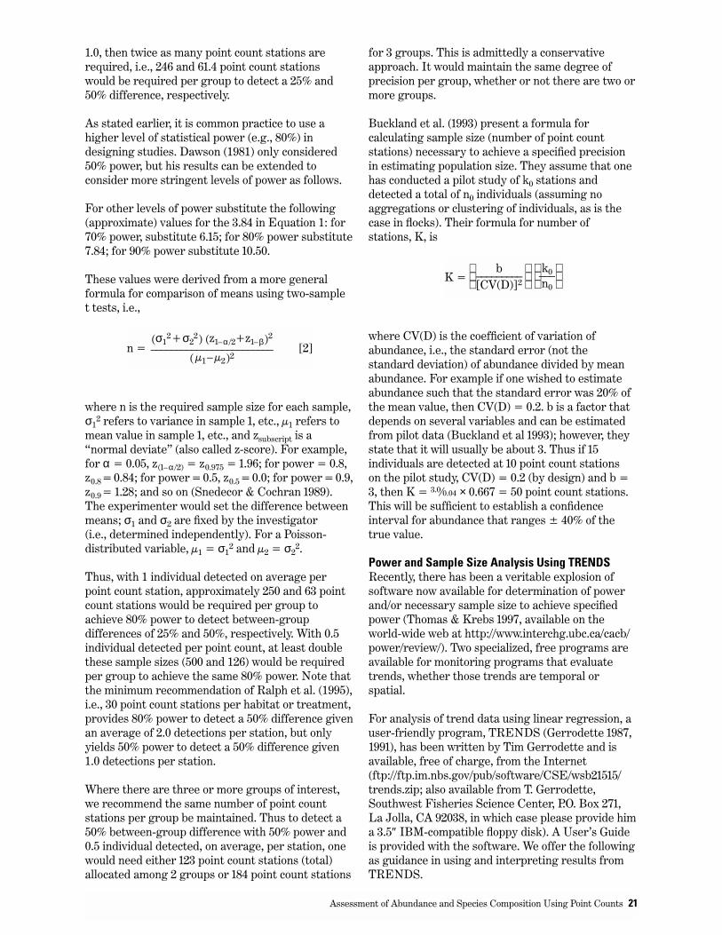
1.0, then twice as many point count stations arerequired, i.e., 246 and 61.4 point count stationswould be required per group to detect a 25% and50% difference, respectively.

As stated earlier, it is common practice to use ahigher level of statistical power (e.g., 80%) indesigning studies. Dawson (1981) only considered50% power, but his results can be extended toconsider more stringent levels of power as follows.

For other levels of power substitute the following(approximate) values for the 3.84 in Equation 1: for70% power, substitute 6.15; for 80% power substitute7.84; for 90% power substitute 10.50.

These values were derived from a more generalformula for comparison of means using two-samplet tests, i.e.,

where n is the required sample size for each sample,σ1

2 refers to variance in sample 1, etc., µ1 refers tomean value in sample 1, etc., and zsubscript is a“normal deviate” (also called z-score). For example,for α = 0.05, z(1–α /2) = z0.975 = 1.96; for power = 0.8,z0.8= 0.84; for power = 0.5, z0.5= 0.0; for power = 0.9,z0.9= 1.28; and so on (Snedecor & Cochran 1989).The experimenter would set the difference betweenmeans; σ1 and σ2 are fixed by the investigator(i.e., determined independently). For a Poisson-distributed variable, µ1 = σ1

2 and µ2 = σ22.

Thus, with 1 individual detected on average perpoint count station, approximately 250 and 63 pointcount stations would be required per group toachieve 80% power to detect between-groupdifferences of 25% and 50%, respectively. With 0.5individual detected per point count, at least doublethese sample sizes (500 and 126) would be requiredper group to achieve the same 80% power. Note thatthe minimum recommendation of Ralph et al. (1995),i.e., 30 point count stations per habitat or treatment,provides 80% power to detect a 50% difference givenan average of 2.0 detections per station, but onlyyields 50% power to detect a 50% difference given1.0 detections per station.

Where there are three or more groups of interest,we recommend the same number of point countstations per group be maintained. Thus to detect a50% between-group difference with 50% power and0.5 individual detected, on average, per station, onewould need either 123 point count stations (total)allocated among 2 groups or 184 point count stations

[2](σ1

2+σ22) (z1–α /2+z1–β)2

________________________( µ1– µ2)2

n =

for 3 groups. This is admittedly a conservativeapproach. It would maintain the same degree ofprecision per group, whether or not there are two ormore groups.

Buckland et al. (1993) present a formula forcalculating sample size (number of point countstations) necessary to achieve a specified precisionin estimating population size. They assume that onehas conducted a pilot study of k0 stations anddetected a total of n0 individuals (assuming noaggregations or clustering of individuals, as is thecase in flocks). Their formula for number ofstations, K, is

where CV(D) is the coefficient of variation ofabundance, i.e., the standard error (not thestandard deviation) of abundance divided by meanabundance. For example if one wished to estimateabundance such that the standard error was 20% ofthe mean value, then CV(D) = 0.2. b is a factor thatdepends on several variables and can be estimatedfrom pilot data (Buckland et al 1993); however, theystate that it will usually be about 3. Thus if 15individuals are detected at 10 point count stationson the pilot study, CV(D) = 0.2 (by design) and b =3, then K = 3.0⁄0.04 × 0.667 = 50 point count stations.This will be sufficient to establish a confidenceinterval for abundance that ranges ± 40% of thetrue value.

Power and Sample Size Analysis Using TRENDSRecently, there has been a veritable explosion ofsoftware now available for determination of powerand/or necessary sample size to achieve specifiedpower (Thomas & Krebs 1997, available on theworld-wide web at http://www.interchg.ubc.ca/cacb/power/review/). Two specialized, free programs areavailable for monitoring programs that evaluatetrends, whether those trends are temporal orspatial.

For analysis of trend data using linear regression, auser-friendly program, TRENDS (Gerrodette 1987,1991), has been written by Tim Gerrodette and isavailable, free of charge, from the Internet(ftp://ftp.im.nbs.gov/pub/software/CSE/wsb21515/trends.zip; also available from T. Gerrodette,Southwest Fisheries Science Center, P.O. Box 271,La Jolla, CA 92038, in which case please provide hima 3.5″ IBM-compatible floppy disk). A User’s Guideis provided with the software. We offer the followingas guidance in using and interpreting results fromTRENDS.

k0 ___ n0

b _________ [CV(D)]2 K =


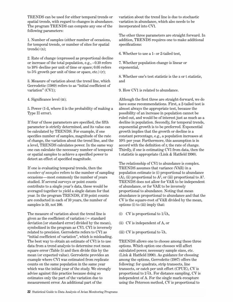
TRENDS can be used for either temporal trends orspatial trends, with regard to changes in abundance.The program TRENDS can compute any one of thefollowing parameters:

1. Number of samples (either number of occasions,for temporal trends, or number of sites for spatialtrends) (n);

2. Rate of change (expressed as proportional declineor increase of the total population, e.g., –0.10 refersto 10% decline per unit of time or space; 0.05 refersto 5% growth per unit of time or space, etc.) (r);

3. Measure of variation about the trend line, whichGerrodette (1989) refers to as “initial coefficient ofvariation” (CV1);

4. Significance level (α);

5. Power (1-ß, where ß is the probability of making aType II error).

If four of these parameters are specified, the fifthparameter is strictly determined, and its value canbe calculated by TRENDS. For example, if onespecifies number of samples, magnitude of the rateof change, the variation about the trend line, and thea level, TRENDS calculates power. In the same wayone can calculate the necessary number of temporalor spatial samples to achieve a specified power todetect an effect of specified magnitude.

If one is evaluating temporal trends, then thenumber of samples refers to the number of samplingoccasions—most commonly the number of yearsstudied. If several surveys or point countscontribute to a single year’s data, these would beaveraged together to yield a single datum for thatyear. In the program TRENDS, if 10 point countsare conducted in each of 10 years, the number ofsamples is 10, not 100.

The measure of variation about the trend line isgiven as the coefficient of variation (= standarddeviation [or standard error] divided by the mean),symbolized in the program as CV1. CV1 is inverselyrelated to precision. Gerrodette refers to CV1 as“initial coefficient of variation”, which is misleading.The best way to obtain an estimate of CV1 is to usedata from a trend analysis to determine root meansquare error (Table 5) and then divide this by themean (or expected value). Gerrodette provides anexample where CV1 was estimated from replicatecounts on the same population in the same yearwhich was the initial year of the study. We stronglyadvise against this practice because doing soestimates only the part of the variation due tomeasurement error. An additional part of the

variation about the trend line is due to stochasticvariation in abundance, which also needs to beincorporated into CV1.

The other three parameters are straight forward. Inaddition, TRENDS requires one to make additionalspecifications:

6. Whether to use a 1- or 2-tailed test,

7. Whether population change is linear orexponential,

8. Whether one’s test statistic is the z or t statistic,and

9. How CV1 is related to abundance.

Although the first three are straight-forward, we dohave some recommendations. First, a 2-tailed test isalmost always the appropriate test, because thepossibility of an increase in population cannot beruled out, and would be of interest just as much as adecline in population. Secondly, for temporal trends,exponential growth is to be preferred. Exponentialgrowth implies that the growth or decline is aconstant percentage, e.g., a population increases at10% per year. Furthermore, this assumption is inaccord with the definition of r, the rate of change.Thirdly, if one is estimating CV1 from data, then thet statistic is appropriate (Link & Hatfield 1990).

The relationship of CV1 to abundance is complex.TRENDS assumes that variance (VAR) in apopulation estimate is (i) proportional to abundance(A), (ii) proportional to A2, or (iii) proportional to A3.TRENDS does not allow for VAR to be independentof abundance, or for VAR to be inverselyproportional to abundance. Noting that meanabundance is proportional to abundance and that theCV is the square-root of VAR divided by the mean,options (i) to (iii) imply that:

(i) CV is proportional to 1/√ A,

(ii) CV is independent of A, or

(iii) CV is proportional to √ A.

TRENDS allows one to choose among these threeoptions. Which option one chooses will affectcalculated power, necessary sample sizes, etc.(Link & Hatfield 1990). As guidance for choosingamong the options, Gerrodette (1987) offers thefollowing: for quadrats, strip transects, linetransects, or catch per unit effort (CPUE), CV isproportional to 1/√ A. For distance sampling, CV isindependent of A. For the single mark-recaptureusing the Peterson method, CV is proportional to


√ A. Presumably, option (i) applies to standard(fixed-distance) point count data, since a pointcount can be thought of as a line transect of lengthzero (Buckland et al. 1993).

Example 5: Power Calculation Using TRENDSTo provide an example of one of the uses ofTRENDS, we consider surveys of Black-headedGrosbeaks (based on data given in Example 3 andFigure 1). CV1 for a single annual count (of log-transformed data) is estimated to be 0.284 (rootmean square error [see Table 5A] divided by meanvalue). Assuming α=0.05, exponential populationchange (i.e., constant percentage change each year),a 2-tailed test, use of the t-statistic, and CV1proportional to 1/√ A, the probability (power) todetect a 5% decline per year after 10 years is 34%.If, instead, CV1 is independent of A, then the powerto detect a 5% decline per year after 10 years is 29%.It is difficult to say whether option (i) or option (ii) ismore appropriate, but the difference between thetwo estimates is small. Thus, the power to detect asubstantial decline (amounting to 40% decline after10 years) is fairly weak. If we increase the time scaleto 15 years, however, power increases to 89% (underoption i). Under this scenario we would haveappreciable power to detect a decline, but after 15years the population will have declined by 54%. Analternative means of increasing power would be toincrease the precision of our annual estimate, whichimplies lowering the variance about the trend line,i.e., decreasing CV1. If CV1 could be lowered from0.284 to 0.200, power would increase (assuming 5%decline over a 10 year period) from 34% to 59%.CV1 might be lowered if sources of error could bereduced (e.g., conduct surveys at the same time ofyear) or if replicate surveys were carried out andthe results for each year then averaged.

One can easily use TRENDS to determine, instead,the minimum number of years required to attain80% power to detect a 5% decline per year (14 years,assuming option i).

Using MONITORWhereas TRENDS uses an analytic approach todetermine sample size, power, etc., MONITOR(developed by James Gibbs) uses computersimulation. Link & Hatfield (1990) argue thatcomputer simulation is to be preferred to analyticsolutions, because the latter can only provideapproximate results. The program MONITOR iseasy to use (ftp://ftp.im.nbs.gov/pub/software/monitor), and a Manual is readily available as well.Users of the program should take into account thefollowing points.

1. Similar to TRENDS, only one data point per plot(or transect or route) is allowed per time unit (e.g.,per year). Unlike TRENDS, MONITOR can allowfor analyses conducted on several plots at once.Where several plots (transects, routes, etc.) areanalyzed at once, MONITOR calculates a weightedtrend (see below for further discussion ofweighting).

2. Whereas “plots”, can refer to “routes” or“transects,” it can also refer to individual point countstations if they will be analyzed in this way (and notsimply pooled across a transect or route). Themaximum number of “plots” is 250.

3. When several surveys are conducted for each plotin the same year (or breeding season or otherinterval of interest), MONITOR averages acrossthese data (i.e., collapsing the data into a single datapoint per plot per year).

4. A critical variable is “variance of plot counts.”This variance is used to simulate variation about thespecified trend line. The manual suggests thatwithin-year variation (determined from multiplesurveys) can be used to estimate between-yearvariance, but this will generally not be valid. Thecorrect estimate is the variance about the trend line,just as with TRENDS.

5. As with TRENDS, the trend can be linear orexponential. We strongly recommend an exponentialtrend for reasons discussed above, unless data athand indicate a linear trend is more appropriate.

6. Data from multiple plots can be weightedaccording to mean abundance, but variance aboutthe plot-specific trends is not used in weighting. Thisis less than satisfactory, because it means that apoorly-estimated trend has as much weight as awell-estimated trend.

7. When data are collected from several plots,MONITOR de-means the values (subtracting offthe mean value for each plot) before calculating thevariance. Otherwise, variance due to habitatdifferences among plots will be included in theestimate of sampling variance (which we areinterested in). However, this de-meaning isundesirable because it over-corrects. That is,suppose we have n plots that are true replicates. Inthis case, all between-plot differences are due tosampling variation, which will have been completelyremoved by de-meaning. A better approach wouldbe to use a covariate (or set of covariates) tocharacterize habitat variation, and then useresiduals from a regression on the habitatcovariate, to provide an appropriate measure ofvariance.


Power and Sample-Size Analyses: Other SourcesSeveral stand-alone statistical packages are nowavailable that can calculate power for a variety ofstatistical tests and situations (reviewed by Thomas& Krebs 1997). In their review, Thomas and Krebsmention five programs that they could recommend.Of these we highlight two: the first is PASS (PowerAnd Sample Size; available from NCSS StatisticalSoftware, 329 North 1000 East, Kaysville, UT 84037;http://www.ncss.com/pass.html). When a class ofecology graduate students was asked to comparePASS with three other recommendable power andsample size programs, 17 out of 19 studentspreferred PASS! It is flexible, accurate, easy to use,and easy to learn. The cost is moderate ($249). Theother program we mention (also reviewed byThomas and Krebs) is GPOWER (Erdfelder et al.1996); though this program did not score as highly asPASS, it is free (http://www.psychologie.uni-trier.de:8000/projects/gpower.html). Thomas andKrebs (1997) examined several general-purposestatistical programs with built-in power analyses,but found none that they could recommend.

Two other valuable sources for power analysis areon the web. The Patuxent Wildlife Research Centerof USGS has an excellent page, that includes apower analysis program for calculating power for monitoring programs, using the data in a manner similar to TRENDS. This is available athttp://www.im.nbs.gov/powcase/powcase.html. Also available is a web page dedicated to thediscussion and calculation of power analyses athttp://www.im.nbs.gov/powcase/powlinks.html. This site has both MONITOR and TRENDSavailable as freeware.

A number of statistical texts treat the problem ofdetermining power. Fleiss (1981) provides anexcellent practical treatment of the problem whenthe outcome is binary (only one of two outcomes), orcan be expressed as a rate or proportion. Thus, histext can be very useful for studies of survival orstudies in which the outcome is presence or absence.Cohen (1988) gives an extensive non-technicaltreatment of power analysis for ANOVA.


Mist-nets can be used to provide estimates of manyparameters: 1. relative abundance, 2. speciescomposition (richness, diversity), 3. productivity, asmeasured by production or abundance of HY(Hatching Year) birds, and 4. annual adult survival.In addition, one can, in theory, estimate 5. offspringsurvivorship to breeding age using data from mist-nets but this is an area that is only now beinginvestigated by researchers. Regarding abundanceand species composition, methods of analysis arethe same as described for analysis of point countdata. Recent examples of analyses of trends inabundance include Johnson & Geupel (1996) andChase et al. (1997); Silkey et al. (1999) discuss thevalidity of inferring population trends from mist-net capture data. Nur et al. (1994) analyzedpatterns of abundance along the upper SacramentoRiver (Example 4) using mist-net capture data andusing point-count data. Mist nets cannot, however,provide an absolute measure of abundance. On theother hand, they can provide an age-specific, andsometimes sex-specific, measure of abundance,with a resolution that cannot be matched by point-count or line-transect data.

Analysis of ProductivityThe number of HY birds caught in a standardizedmist-netting study can provide an index ofproduction of young (DeSante & Geupel 1987, Nur& Geupel 1993b, DeSante et al. 1993). Such datahave been analyzed in three ways: (i) analysis oftotal number of HY birds caught; (ii) analysis ofnumber of HY birds caught per AHY (AfterHatching Year, i.e., adult) caught; or (iii) analysis ofper cent of all birds who are HY. Among theseparameters, (iii) is just a transformation of (ii), andvice versa, provided that all birds are classified asHY or AHY (total = AHY + HY). This can be seenas follows: let HY/AHY=R. Then proportion of allbirds that are HY = HY/(AHY + HY), can bewritten as

Thus, (iii) only re-expresses (ii), but theinterpretation of (ii) is more direct: the numberof fledged young per adult.

1proportion HY = _______1 + (1–R)

Nur & Geupel (1993a, 1993b) point out that there arehazards with including the number of AHY birdscaught as a measure of productivity (as do indices iiand iii above): notably, the catchment area of HYand AHY can differ markedly (Nur & Geupel 1993a).Secondly, many AHY birds are transient, i.e., notbreeding locally. As an alternative, one can use themeasure in (i), HY birds alone. If one findsdifferences in the number of HY birds caught in twosets of sites, or can establish a trend in HY numbers,this provides information about the production ofyoung on a population level, but it may or may notindicate differences or trends in productivity perpair. Thus we recommend that, if variations inbreeding population size can safely be ruled out, incomparing areas or comparing years, the number ofHY be analyzed by itself (see examples in Nur &Geupel 1993b). Otherwise, the biologist shouldanalyze (ii) or (iii). Example 6 demonstratesdifferent ways of analyzing productivity.

Example 6: Analyses of Productivity.This example is taken from the study of the impactof the herbicide metam sodium on landbirdpopulations of the Sacramento River, described inExample 4. Table 8 shows a species-by-speciesanalysis of productivity as measured in two ways,HY birds per 100 net-hours, and proportion of HYbirds in the catch.

To examine patterns of productivity we selectedthose species with sufficient sample size. Ourcriteria were: (1) at least 36 individuals caught (of allage classes) from the 9 sites, and (2) at least 12 HYindividuals caught, total, from the 9 sites. Six speciesmet both criteria (Table 8). The “36 individualcriterion” implied that each site averaged 4 or moreindividuals caught, which we considered a minimalacceptable number. We would have preferred toimpose a minimum of 45 individuals (i.e., 5individuals caught per site on average), but then wewould have had fewer than 6 species to analyze. Thesecond criterion, at least 12 HY individuals caughtamong the 9 sites, may seem too low a threshold (anaverage of 1.33 HY individuals caught per site).Nevertheless, we wished to include possibleinstances where reproductive success was poor or

25

III. Demographic Monitoring: Mist-nets

nil at a number of the 9 sites; such apparentreproductive failure might be especially informative.Thus, a hypothetical species with 5, 4, 2, 1, 0, 0, 0, 0, 0captures at 9 sites would qualify with respect to the“12 HY” criterion. On the other hand, a species with12 HY captures at 1 site, and 8 sites without any HYcaptures is not particularly informative. We thus seta 3rd criterion: HY captures at a minimum of 3 sites.All species that met criteria (1) and (2), also met the3rd criterion.

To analyze the HY capture data, we log-transformedcapture rates (birds caught per 100 net-hours), foreach species at each site. To avoid taking the log of 0(which is undefined), we added a constant—in thiscase, 1—before log-transforming. Had there been nozeroes in the data set, we would not have added any

constant; there would have been no need to. Whereasadding a constant before log-transformation isstandard practice, it can lead to bias (Thomas 1996).However, the direction of bias is conservative: addinga constant makes it somewhat more difficult to detectan effect (e.g., to detect a trend). We recommend thatinvestigators try two different constants (e.g., adding0.5 and adding 1) and determine if results are similar.If they are, then the investigator has some confidencethat his or her results are not unduly sensitive to thechosen constant.

For analysis of the proportion of HY in the catch, weused the logit-transformation. In the case wheretotal captures = HY + AHY,

logit(proportion of HY) = loge(HY/AHY).


Table 8. Analysis of mist-net captures, Sacramento River 1993: Relationship to Damage Index for the six species with adequate sample size (at least 12 HY individuals caught, and at least 36 individuals, total, caught, among 9 sites).

A) Dependent Variable: Hatching Year birds per 100 net hoursa

Species Analysis Number HY Caught

Black-headed Grosbeak ß = –0.369 ± 0.192, P = 0.096, R2a= 0.251, R2= 0.345 12McGillivray’s Warbler ß = –0.519 ± 0.405, P = 0.240, R2a= 0.074, R2= 0.190 39Orange-crowned Warbler ß = –0.226 ± 0.078, P = 0.023, R2a= 0.479, R2= 0.544 15Song Sparrow ß = –0.565 ± 0.357, P = 0.16, R2a= 0.159, R2= 0.264 55Spotted Towhee ß = –0.649 ± 0.227, P = 0.024, R2a= 0.472, R2= 0.538 32Yellow-breasted Chat ß = –0.462 ± 0.169, P = 0.029, R2a= 0.449, R2= 0.518 13

B) Dependent Variable: Proportion of Hatching Year birdsb

Species Analysis Number of Sites

Black headed Grosbeak ß = –0.901 ± 0.566, P = 0.15, R2a= 0.161, R2= 0.266 9McGillivray’s Warbler ß = –1.054 ± 1.115, P > 0.3, R2a= 0.006, R2= 0.130 9Orange-crowned Warbler ß = +1.623 ± 0.432, P = 0.007, R2a= 0.622, R2= 0.669 9Song Sparrow ß = –0.819 ± 0.690, P > 0.2, R2a= 0.170, R2= 0.274 9Spotted Towhee ß = –1.707 ± 0.789, P = 0.074, R2a= 0.344, R2= 0.438 8Yellow-breasted Chat ß = –1.497 ± 1.117, P > 0.2, R2a= 0.117, R2= 0.264 7

a Hatching Year Birds caught per 100 net-hours, log-transformed, i.e. ln((HY caught + 1)/100 net-hours). Results of simple regressionanalyses for effect of Vegetation Damage Index. Sample size = 9 sites for each analysis.b Proportion of Hatching Year birds, logit-transformed Results of simple regression analyses for effect of Vegetation Damage Index.Sample size (number of sites) for each analysis is shown.

Table 9. Analysis of mist-net captures, Sacramento River, 1993: Relationship of HY, and proportion HY birdscaught in relation to Vegetation Damage Index. Results of simple regression analyses; independent variablein each model is Vegetation Damage Index. Number of sites (sample size) is 9. Capture rates have beenlog-transformed, i.e. ln((number of birds + 1)/100 net-hours).

Dependent Variable Analysis

HY birds/100 net-hours ß = –0.795 ± 0.201, P = 0.006, R2a= 0.646, R2= 0.690Proportion of HY birds caught logit-transformed ß = –0.360 ± 0.120, P = 0.028, R2a= 0.453, R2= 0.521

The logit transformation is a commonly usedtransformation in biological analysis and forms thebasis of logistic regression (Chapter V). Note thatthe logit(proportion of HY) is undefined when thedenominator (in this case number AHY caught) iszero. We could have added a constant to thedenominator to avoid this “problem” but did not;we consider it biologically appropriate that ourmeasure of productivity is undefined when thereare (apparently) no adults present. For the analysisin Table 8B, sites could not be included wherelogit(proportion of HY) was undefined, i.e., whereno AHY were caught. This applied to two of thesix species.

As shown in Table 8, of the six species analyzed,three showed a significant decline in capture ratewith increasing biological damage. Analyses of theHY/AHY ratio indicated a consistently downwardtrend with increasing damage (5 out of 6 species hada negative slope), but no species had a significantnegative trend. These results suggest that samplesizes of individual species were likely too small toreveal significant patterns, and a pooled analysiswas carried out, shown in Table 9. Analyses of allHY and AHY caught for all terrestrial bird specieswere pooled and the results confirmed a significantdecrease in productivity with increase in damagesymptoms.

Analysis of Adult SurvivalSurvival can be analyzed in two ways: using capture/recapture methods or analyzing “returnrate”. Return rate is the proportion of individualsobserved in one time period (we refer to this period as t), which are observed again (resighted,recaptured, etc.) in the following time period (period t + 1). Thus return rate is the product of twoprocesses: survival from period t to period t + 1, andresighting (or recapture) in period t + 1. Resightingprobability is defined as the probability an individualis resighted at time t + 1, given that an individualhas survived until time t + 1 (Clobert et al. 1987,Nur & Clobert 1988). In short,

return rate = survival × recaptureprobability .probability.

(We use “recapture” in a broad sense to refer toboth resighting and recapture.) The justification for analyzing return rate as a means of studyingsurvival is the assumption that recapture probabilityis 100% or, at least, that it can be treated as aconstant. This assumption is likely to be violatedwhen one is comparing the sexes, or comparingdifferent species or even different populations.Capture/recapture methodology analyzes bothparameters, survival and recapture probability.

In this way, survival can be estimated independentlyof recapture probability and one can test fordifferences in survival as well as differences inrecapture probability (Lebreton et al. 1992). Itwould seem that capture/recapture methodologyprovides a superior means to analyze survival and,in theory, it does. However, there are threedrawbacks to its usage:

1. Capture/recapture methods require at least threefield seasons to estimate survival for one year,instead of two. 2. More data are required to carryout these analyses than with return-rate analyses,because two parameters are being estimated insteadof one. 3. The optimal software for survival analysesis not yet available, one that combines flexibility,statistical power, and ease of use, without requiringspecialized instruction. In the meantime, there areseveral programs available which can fill the gap (formore detailed discussion, see Lebreton et al. 1993).Table 10 summarizes statistical programs that areavailable for analyzing capture/recapture data(based on Lebreton et al. 1992). Below we discuss sixprograms that have been widely used (SURGE,RELEASE, MARK, SURPH, JOLLY, andJOLLYAGE).

General Comments. Capture/recapture models such as SURGE require at least three field seasons(usually years) in order to estimate survival betweenthe first season and the second, though it is possible,making some assumptions, to derive survivalestimates for the period between the second andthird field seasons. Thus ten field seasons wouldyield estimates of survival for each of eight years,and so on. It is strongly recommended that thecapture occasions be equally spaced and generallyspeaking the programs SURGE, RELEASE,JOLLY, and JOLLYAGE assume this. If one isseeking to estimate annual survival, then thecapture “occasion” is the year or breeding season. In each year, an individual is either caught or re-sighted (scored a “1”), or not observed (scored a“0”). This allows one to construct a capture historyfor each individual (a string of 1’s and 0’s). Thecapture history data set consists of rows ofindividual capture histories. The capture occasionscould instead be defined time periods within a singleyear. This would allow one to estimate survivalwithin a year. In most survival analyses of constant-effort mist-netting data (Peach 1993, Chase et al.1997), all captures for each species from a singlebreeding season have been pooled.

SURGE. This program is available from AVENIX(14, Avenue de Montpellier, 34680 SAINT-GEORGES-D’ORQUES, France; fax number (33) 67 40 22 90. The program comes with a user’smanual (Pradel & Lebreton 1993), and runs on

Demographic Monitoring: Mist-nets 27

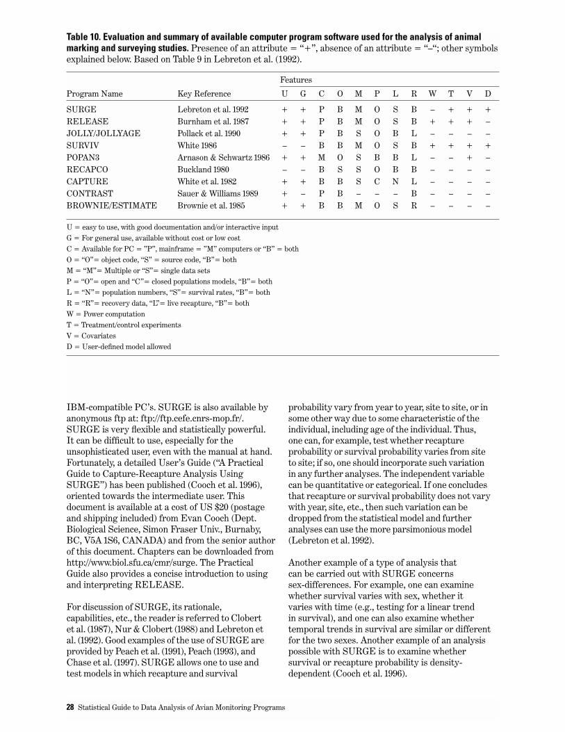
IBM-compatible PC’s. SURGE is also available byanonymous ftp at: ftp://ftp.cefe.cnrs-mop.fr/.SURGE is very flexible and statistically powerful. It can be difficult to use, especially for theunsophisticated user, even with the manual at hand.Fortunately, a detailed User’s Guide (“A PracticalGuide to Capture-Recapture Analysis UsingSURGE”) has been published (Cooch et al. 1996),oriented towards the intermediate user. Thisdocument is available at a cost of US $20 (postageand shipping included) from Evan Cooch (Dept.Biological Science, Simon Fraser Univ., Burnaby,BC, V5A 1S6, CANADA) and from the senior authorof this document. Chapters can be downloaded fromhttp://www.biol.sfu.ca/cmr/surge. The PracticalGuide also provides a concise introduction to usingand interpreting RELEASE.

For discussion of SURGE, its rationale,capabilities, etc., the reader is referred to Clobertet al. (1987), Nur & Clobert (1988) and Lebreton etal. (1992). Good examples of the use of SURGE areprovided by Peach et al. (1991), Peach (1993), andChase et al. (1997). SURGE allows one to use andtest models in which recapture and survival

probability vary from year to year, site to site, or insome other way due to some characteristic of theindividual, including age of the individual. Thus,one can, for example, test whether recaptureprobability or survival probability varies from siteto site; if so, one should incorporate such variationin any further analyses. The independent variablecan be quantitative or categorical. If one concludesthat recapture or survival probability does not varywith year, site, etc., then such variation can bedropped from the statistical model and furtheranalyses can use the more parsimonious model(Lebreton et al. 1992).

Another example of a type of analysis that can be carried out with SURGE concerns sex-differences. For example, one can examinewhether survival varies with sex, whether it varies with time (e.g., testing for a linear trend in survival), and one can also examine whethertemporal trends in survival are similar or differentfor the two sexes. Another example of an analysispossible with SURGE is to examine whethersurvival or recapture probability is density-dependent (Cooch et al. 1996).


Table 10. Evaluation and summary of available computer program software used for the analysis of animalmarking and surveying studies. Presence of an attribute = “+”, absence of an attribute = “–“; other symbolsexplained below. Based on Table 9 in Lebreton et al. (1992).

Features

Program Name Key Reference U G C O M P L R W T V D

SURGE Lebreton et al. 1992 + + P B M O S B – + + +RELEASE Burnham et al. 1987 + + P B M O S B + + + –JOLLY/JOLLYAGE Pollack et al. 1990 + + P B S O B L – – – –SURVIV White 1986 – – B B M O S B + + + +POPAN3 Arnason & Schwartz 1986 + + M O S B B L – – + –RECAPCO Buckland 1980 – – B S S O B B – – – –CAPTURE White et al. 1982 + + B B S C N L – – – –CONTRAST Sauer & Williams 1989 + – P B – – – B – – – –BROWNIE/ESTIMATE Brownie et al. 1985 + + B B M O S R – – – –

U = easy to use, with good documentation and/or interactive inputG = For general use, available without cost or low costC = Available for PC = ”P”, mainframe = ”M” computers or “B” = bothO = “O”= object code, “S” = source code, “B”= bothM = “M”= Multiple or “S”= single data setsP = “O”= open and “C”= closed populations models, “B”= bothL = “N”= population numbers, “S”= survival rates, “B”= bothR = “R”= recovery data, “L”= live recapture, “B”= bothW = Power computationT = Treatment/control experimentsV = CovariatesD = User-defined model allowed

Example 7: Recapture Probability and Territory StatusThe following example is taken from Nur & Geupel(1993a). Survival of Wrentits (Chamaea fasciata), ahighly sedentary species, caught in standardizedmist-netting at the Palomarin field station, wasassessed over an 11 year period (1980 to 1991). Therewas no significant year-to-year variation in survivalprobability or recapture probability. Survival andrecapture probabilities were analyzed for twodifferent classes of individuals: (1) known territoryholders and (2) individuals not holding territories(floaters). Additional data indicated that mostfloaters were very transient. The results of theSURGE analysis are shown in Table 11 for the twoclasses of individuals (territory holders and floaters)and for all individuals, pooled. The results indicatethe value of distinguishing individuals with high sitefidelity (territory holders) from transientindividuals. Survival of territory holders wasestimated to be 57%. But when territory holders andfloaters were pooled, the survival estimate was muchlower at 31%. The reason was that recaptureprobability was very different for the two groups:71% for territory holders and 5% for floaters. Whenthese two groups were pooled, thus violating theassumption of equal survival and recaptureprobability among individuals, the result was a poorestimate of recapture probability and thus anunreliable estimate of survival.

The other programs: RELEASE, MARK, JOLLY,and JOLLYAGE, are freely available to the public(RELEASE and MARK: G.C. White, Dept ofFishery & Wildlife Biology, Colorado State Univ.,Fort Collins, CO 80523; JOLLY and JOLLYAGE:J.E. Hines, Patuxent Wildlife Research Center,Laurel, MD 20708).

RELEASE. The program is described in Burnhamet al. (1987). The program itself is fairly easy to use.It can estimate and compare survival among groupsas well as conduct goodness-of-fit tests to determineif assumptions of analyses are being met (e.g., there

is no heterogeneity in capture probability amongindividuals, there is no recapture-avoidance). Amajor drawback is that no easy to use manual isavailable. Those who wish to use RELEASE toconduct goodness-of-fit tests are urged to consultthe Practical Guide to SURGE (Cooch et al. 1996)where RELEASE is treated in the Appendix.

MARK. This program is in final-development stage.A beta-test version is available fromhttp://www.cnr.colostate.edu/~gwhite/mark/mark.htm. No User’s Manual as such is available butdocumentation is available from the same source.This program is menu-driven and provides anexcellent combination of flexibility, power, and ease-of-use. One disadvantage of MARK is that it isdesigned only to run on Windows95. Novices incapture/recapture analysis are recommended toconsult the Practical Guide to SURGE (Cooch et al.1996), where much of the rationale and backgroundmaterial for this body of analysis is presented.

SURPH (SURvival under Proportional Hazards).This program can be used to analyze survival rates, using both capture-recapture data, and usingknown fate data (also called time to death or time to failure data). SURPH has been developed bySteven G. Smith, John R. Skalski and others. For more information, direct enquiries [email protected]; also see the web site:http://www.cqs.washington.edu/surph/index.html. An extensive, informative, and easy to use manual isavailable. In general, the program is easy to use andflexible. One of its greatest strengths is that, unlikeother capture-recapture programs discussed, itallows one to analyze the effects of individual-levelcovariates on survival and recapture probability.Body mass of adults at the time of first capture ordate of fledging are two possible examples ofindividual level covariates.

JOLLY and JOLLYAGE. These programs aredescribed in Pollock et al. (1990). These twoprograms are the least sophisticated of thosediscussed. The main features to recommend them


Table 11. Results of SURGE analysis of Wrentits, by territory status.

Survival Probability Recapture Probability

Per cent 95% C.I. Per cent 95% C.I.

Territory holders 57a 47-67 71b 53-84Non-territory holders (floaters) 38a 13-72 5b 1-18All adults, pooled 31 22-41 38 23-56

a Difference in parameter estimates, territory holders vs. floaters: P > 0.3b Difference in parameter estimates, territory holders vs. floaters: P < 0.0001

are that they are easy to obtain, easy to use, and themanual for their use (Pollock et al. 1990) is relativelyeasy to follow. One advantage of these two programsis that, unlike the above-discussed programs, JOLLYand JOLLYAGE also estimate population size.

JOLLY assumes no age differentiation (i.e., all ageshave similar survival and recapture probability);JOLLYAGE allows for two age-classes. (In contrast,there is no limitation to the number of age classesconsidered in SURGE.) JOLLY allows a choicebetween one of five models (Table 12). In model A,survival (symbolized phi) and recapture probability(symbolized p) are both time-specific (e.g., they varyfrom year to year). Model A' is like model A but itallows for deaths only, and no new recruitment,whether by birth or by immigration. Thus, model A'would not apply to an investigation that spans morethan 1 year. In model B, survival is time-specific andcapture probability is not, it is constant. In model Dboth survival and capture probability are constantwith time. There is no model C, corresponding toconstant survival, recapture probability varyingwith time. The fifth model is referred to as model 2.(No, there is no model 1.) This model is appropriateif there is trap-shyness (i.e., net avoidance) followingfirst capture. In this case, the program does not useinformation from individuals between their firstcapture and the subsequent capture period. It isassumed that by the time of the second captureperiod following first capture, trap-shyness hasdisappeared. The disadvantage of model 2 is that asizable portion of the data are excluded fromcalculations of survival and capture probability.

JOLLYAGE incorporates three of the above models,adapted to two age classes: these are referred to asA2, B2 and D2. In all these models, survival, but notcapture probability is allowed to vary between theage classes. JOLLY and JOLLYAGE allowgoodness-of-fit tests for a particular model. All theprograms discussed above calculate confidenceintervals. However, JOLLY and JOLLYAGE allowthe upper confidence limit for capture or survival

probability to exceed 1.0 (which is impossible) andallow the lower limit to be less than 0.0 (which is alsoimpossible).

DesignPlacement of nets and mist-net stations is describedby Ralph et al. (1993) and DeSante et al. (1993).Different design considerations apply to the study ofproductivity as compared to the study of adultsurvival. In the case of productivity, the unit ofanalysis is the mist-net station, often containing 10mist-nets. With pilot data in hand, one candetermine the minimum number of mist-net stationsneeded to achieve acceptable statistical power orprecision. Analyses can be conducted, either onindividual species (DeSante et al. 1993, Nur et al.1994, Johnson and Geupel 1996, Chase et al. 1997) oron groups of species (DeSante and Geupel 1987);examples of both methods were described inExample 4. Power will strongly depend on thenumber of individuals caught per station. Clearly,pooling species (e.g., on the basis of habitatpreference), will improve statistical power. Foranalyses of productivity, power, and necessarysample size to achieve a stated level of power, can becalculated with standard methods (see above). Foranalysis of linear trends in space or time, the readercan use specialized programs, such as TRENDS andMONITOR, described above, or use a more generalprogram, such as PASS.

For analyses of adult survival, the unit of analysis isthe individual bird (adult). More precisely, the unitof analysis is the individual capture/recapturehistory. Since recapture is a binary event—anindividual is either recaptured or it is not—powerand necessary sample size can be estimated,adapting methods and results from such binaryprocesses. Fleiss (1981) provides an easy to use text.To estimate necessary sample size (here, number ofdifferent individuals initially caught), it is necessaryto know the average recapture rate (among allindividuals caught in a given year, the proportion ofindividuals recaught in a subsequent year).


Table 12. Summary of models in JOLLY and JOLLYAGE (Pollack et al. 1990).

Program Model Parameters Description

JOLLY A phii, pi Full Jolly-Seber modelA' phii, pi Jolly-Seber “death only” modelB phii, p Time-specific survival and constant capture probablityD phi, p Constant survival and capture probability2 phii, phi*i, pi Jolly-Seber model with “trap-response”

JOLLY AGE A2 phii, phii', pi 2-age, time-specific survival and capture probabilityB2 phi, phi', pi 2-age, constant survival, time-specific capture probabilityD2 phi, phi', p 2-age, constant survival and capture probability

Preliminary results from the Palomarin Fieldstation (Nur & Geupel 1993a, Chase et al. 1997,Geupel and Nur unpublished data) and elsewhere(DeSante et al. 1993), indicate that, under favorableconditions, 30% of adults caught in one year can beexpected to be recaught in the next year. We assumethat transient individuals (see below) are eliminatedfrom the analysis. The recapture rate may easily begreater or less than that, but is likely to varybetween 20 and 45%.

Fleiss (1981) gives an extensive table fordetermining sample size necessary to detectsignificant effects, as a function of the recapture rate(here assumed to be proportional to survival) of twogroups—e.g., two different treatments or twohabitats. For example, if recapture rate of group 1 is0.20 and the recapture rate of group 2 is 0.40 (i.e.,group 2 is twice as likely to be recaught as group 1),the necessary sample to achieve 80% power todetect an effect at the 0.05 level is 91 for each group,or 182 in total. This would represent about 55recaptured individuals, in all (=182 × .3). If one werewilling to settle for 50% power, one could drop thesample size to 50 individuals caught for each group.Also, if one wished to detect a significant difference,with 80% power, when one group is 50% more likelyto survive than another, while keeping the averagerecapture rate at 30% (i.e., recapture of 24% vs.36%), this would require sample sizes of 323individuals for each group (or 646, in total). Theseresults and others summarized in Fleiss (1981) canprovide guidance in designing a study. In somecases, the desired sample size will probably beachieved by using data over multiple years.

As noted above, capture-recapture analyses requiremore data than many other types of analysis. This isso for two reasons: (1) more data are required toestimate two parameters (survival and captureprobability are separately estimated) than just oneparameter, and (2) capture-recapture analyses relyon maximum-likelihood methods, unlike ANOVA andlinear regression, which do not (Kleinbaum et al.1988). The maximum-likelihood method can only

work as intended when the estimate in question isgreater than 0 and less than 1, assuming we areconsidering probability estimates, whose minimumand maximum are 0 and 1. That is, the methodbreaks down when an estimate falls on a boundary(in this case 0 or 1). Examples where this boundaryproblem comes up are: (i) you band 20 individuals ofspecies x and none are ever recaptured, or (ii) all 20individuals of species x are recaptured. It may seemunlikely that during the course of a multi-year studyone obtains 0% recaptures or 100% recaptures, butsuch outcomes are not unlikely on a year-by-yearbasis. Thus, sampling error alone can lead to asituation where all individuals captured in aparticular year are either re-sighted or noindividuals are re-sighted. This presents a problemif one wishes to examine year-by-year variation insurvival.

Problems can also arise in estimating captureprobability. Suppose 20 individuals are captured andreleased in year 1. In year 2, five of these individualsare recaught, and in year 3, two of the five arerecaught a second time. However, 15 of those caughtand released in year 1 are never seen in year 2 oryear 3. We don’t know how many of those 15 actuallydied by year 2 and how many were alive but weremissed that year. If there were one or moreindividuals caught in year 1, missed in year 2, andthen caught again in year 3 (or later), we would haveenough information to try and estimate captureprobability. But in the example given, the capture-recapture analysis is forced to estimate that thecapture probability is 100%. That estimate isproblematic, first because it presents difficulty forthe maximum likelihood method, and second,because such an estimate is likely to be biologicallyincorrect. We therefore recommend that capture-recapture analyses be conducted on data sets thathave at least one (but preferably more than one)individual with gaps in their recapture histories (e.g. “101” or “1001”). Here “dataset” would refer tocaptures from a single species at a single site. Thereader is referred to Cooch et al. (1996) for furtherdiscussion.


Nest-monitoring provides detailed information on anumber of different aspects of reproductive success,in addition to potentially providing information ondensity, habitat associations, and other ecologicalcharacteristics (Table 1). The following componentsof reproductive success of a particular species maybe studied: clutch initiation dates (or other aspectsof breeding season chronology), number of nestattempts and/or broods reared per pair, clutch size,brood size, hatchability (proportion of eggs thathatch), number of young fledged, number of youngfledged per pair, proportion of nests that fail, andnest survivorship (Martin 1992, Martin and Geupel1993, Ralph et al. 1993). In this section we limitattention to nest survivorship. With regard to theother elements of reproductive success, theiranalysis is relatively straight forward and does notpresent any unusual difficulties. Some of thesecomponents of reproductive success can be analyzedusing standard linear model analysis. Theassumptions of such analysis must be met, forexample, the assumption that residuals are normallydistributed. Where the outcome is binary, e.g., abrood is scored “0” if it fails to produce young, and“1” if it produces one or more young, logisticregression (Chapter V) can be used. The reader isreferred to several recent papers which haveanalyzed reproductive success (Geupel & DeSante1990, Martin 1992, Sherry & Holmes 1993, Nur &Geupel 1993b, Robinson et al. 1995).

BackgroundIn nest-monitoring studies, analysis of nestsurvivorship is usually carried out by the Mayfieldmethod (Mayfield 1961, Mayfield 1975). Importantcontributions to these analysis were made byJohnson (1979) and Hensler & Nichols (1981).Recently, Pollock & Cornelius (1988) and Bromaghin& McDonald (1993) have developed alternativemethods. We discuss two methods that provide goodalternatives to the Mayfield method, though neitherhas yet been widely adopted. The first is the methodof Bromaghin & McDonald (1993), which they call“Systematic Nest-searching,” and the second isoften termed “time-to-failure” analysis. However,the Mayfield (1961, 1975) method is at present themost widely used.

AnalysisIf all nests are discovered upon initiation (e.g.,before egg-laying has begun) and then followed untilthey succeed or fail, then it is not necessary to usethe Mayfield method to estimate nest survivorship.In that case, one can score each nest as successful ornot, and data can be analyzed with logisticregression, discriminant analysis or other methods.However, for many field studies, nests are usuallyfound at various stages of the nesting cycle, and,furthermore, the ultimate fate of each nest is notalways known. With such incomplete information, itis recommended to use the Mayfield (1961, 1975)method to estimate nest survivorship (but see belowfor analytic methods that assume that nests can beaged upon discovery). The Mayfield method consistsof dividing the number of nests known to have failedby the sum of the number of days during whichnests were observed and at risk of failing (equals“exposure-days”). This provides an estimate of dailynest mortality and is used to estimate nestsurvivorship for a particular stage of the nestingperiod (if one wishes to estimate stage-specificsurvival probability) or for the entire nesting period.

We consider it useful to summarize the followingguidelines to facilitate nest survivorship analysisbased on Mayfield (1961, 1975). To be included incalculations of nest success a nest must be observeda minimum of 2 times and the outcome (its fate)must be known, or at least must be established forthe last observation of that nest.

Typically the nesting period is divided in to threestages: egg laying, incubation, and nestling periods.Occasionally nest building is differentiated as afourth stage; however, in the absence of observedeggs it is difficult to distinguish early predationfrom failure to lay eggs. Therefore, nestsurvivorship is normally only determined from thepoint that the first egg is laid (or as soon as possiblethereafter). For most passerines, one egg is laid perday, and incubation assumed to begin when the lastegg is laid, with the nestling period beginning whenthe first egg hatches. In general, when there is noother information, the mid-point between nestchecks is used as an estimate of the timing ofsignificant events occurring in the nesting cycle. It is important to check nests regularly (once every

32

IV. Demographic Monitoring: Nest-monitoring

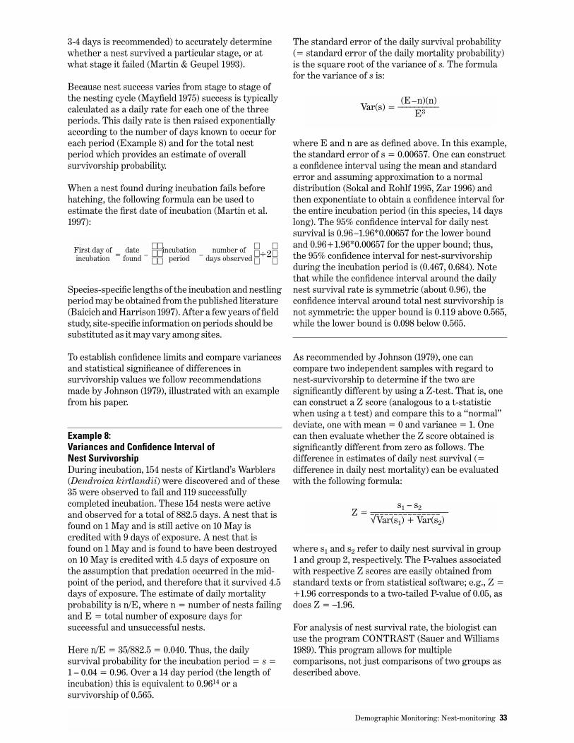
3-4 days is recommended) to accurately determinewhether a nest survived a particular stage, or atwhat stage it failed (Martin & Geupel 1993).

Because nest success varies from stage to stage ofthe nesting cycle (Mayfield 1975) success is typicallycalculated as a daily rate for each one of the threeperiods. This daily rate is then raised exponentiallyaccording to the number of days known to occur foreach period (Example 8) and for the total nestperiod which provides an estimate of overallsurvivorship probability.

When a nest found during incubation fails beforehatching, the following formula can be used toestimate the first date of incubation (Martin et al.1997):

÷2

Species-specific lengths of the incubation and nestlingperiod may be obtained from the published literature(Baicich and Harrison1997). After a few years of fieldstudy, site-specific information on periods should besubstituted as it may vary among sites.

To establish confidence limits and compare variancesand statistical significance of differences insurvivorship values we follow recommendationsmade by Johnson (1979), illustrated with an examplefrom his paper.

Example 8: Variances and Confidence Interval ofNest SurvivorshipDuring incubation, 154 nests of Kirtland’s Warblers(Dendroica kirtlandii) were discovered and of these35 were observed to fail and 119 successfullycompleted incubation. These 154 nests were activeand observed for a total of 882.5 days. A nest that isfound on 1 May and is still active on 10 May iscredited with 9 days of exposure. A nest that isfound on 1 May and is found to have been destroyedon 10 May is credited with 4.5 days of exposure onthe assumption that predation occurred in the mid-point of the period, and therefore that it survived 4.5days of exposure. The estimate of daily mortalityprobability is n/E, where n = number of nests failingand E = total number of exposure days forsuccessful and unsuccessful nests.

Here n/E = 35/882.5 = 0.040. Thus, the dailysurvival probability for the incubation period = s =1 – 0.04 = 0.96. Over a 14 day period (the length ofincubation) this is equivalent to 0.9614 or asurvivorship of 0.565.

incubation number of period – days observed

First day of dateincubation = found –

The standard error of the daily survival probability(= standard error of the daily mortality probability)is the square root of the variance of s. The formulafor the variance of s is:

where E and n are as defined above. In this example,the standard error of s = 0.00657. One can constructa confidence interval using the mean and standarderror and assuming approximation to a normaldistribution (Sokal and Rohlf 1995, Zar 1996) andthen exponentiate to obtain a confidence interval forthe entire incubation period (in this species, 14 dayslong). The 95% confidence interval for daily nestsurvival is 0.96–1.96*0.00657 for the lower boundand 0.96+1.96*0.00657 for the upper bound; thus,the 95% confidence interval for nest-survivorshipduring the incubation period is (0.467, 0.684). Notethat while the confidence interval around the dailynest survival rate is symmetric (about 0.96), theconfidence interval around total nest survivorship isnot symmetric: the upper bound is 0.119 above 0.565,while the lower bound is 0.098 below 0.565.

As recommended by Johnson (1979), one cancompare two independent samples with regard tonest-survivorship to determine if the two aresignificantly different by using a Z-test. That is, onecan construct a Z score (analogous to a t-statisticwhen using a t test) and compare this to a “normal”deviate, one with mean = 0 and variance = 1. Onecan then evaluate whether the Z score obtained issignificantly different from zero as follows. Thedifference in estimates of daily nest survival (=difference in daily nest mortality) can be evaluatedwith the following formula:

where s1 and s2 refer to daily nest survival in group1 and group 2, respectively. The P-values associatedwith respective Z scores are easily obtained fromstandard texts or from statistical software; e.g., Z =+1.96 corresponds to a two-tailed P-value of 0.05, asdoes Z = –1.96.

For analysis of nest survival rate, the biologist canuse the program CONTRAST (Sauer and Williams1989). This program allows for multiplecomparisons, not just comparisons of two groups asdescribed above.

s1 – s2Z = ___________________√Var(s1) + Var(s2)

(E–n)(n)Var(s) = __________

E3

Demographic Monitoring: Nest-monitoring 33

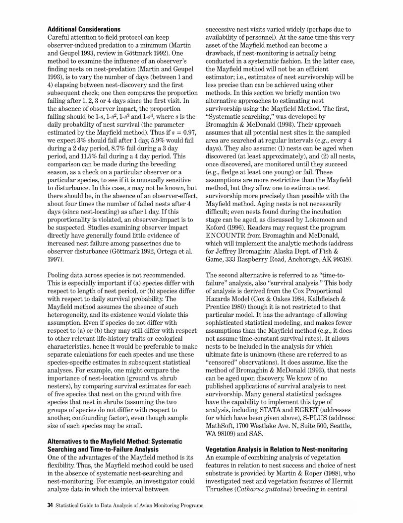
Additional ConsiderationsCareful attention to field protocol can keepobserver-induced predation to a minimum (Martinand Geupel 1993, review in Göttmark 1992). Onemethod to examine the influence of an observer’sfinding nests on nest-predation (Martin and Geupel1993), is to vary the number of days (between 1 and4) elapsing between nest-discovery and the firstsubsequent check; one then compares the proportionfailing after 1, 2, 3 or 4 days since the first visit. Inthe absence of observer impact, the proportionfailing should be 1-s, 1-s2, 1-s3 and 1-s4, where s is thedaily probability of nest survival (the parameterestimated by the Mayfield method). Thus if s = 0.97,we expect 3% should fail after 1 day, 5.9% would failduring a 2 day period, 8.7% fail during a 3 dayperiod, and 11.5% fail during a 4 day period. Thiscomparison can be made during the breedingseason, as a check on a particular observer or aparticular species, to see if it is unusually sensitiveto disturbance. In this case, s may not be known, butthere should be, in the absence of an observer-effect,about four times the number of failed nests after 4days (since nest-locating) as after 1 day. If thisproportionality is violated, an observer-impact is tobe suspected. Studies examining observer impactdirectly have generally found little evidence ofincreased nest failure among passerines due toobserver disturbance (Göttmark 1992, Ortega et al.1997).

Pooling data across species is not recommended.This is especially important if (a) species differ withrespect to length of nest period, or (b) species differwith respect to daily survival probability. TheMayfield method assumes the absence of suchheterogeneity, and its existence would violate thisassumption. Even if species do not differ withrespect to (a) or (b) they may still differ with respectto other relevant life-history traits or ecologicalcharacteristics, hence it would be preferable to makeseparate calculations for each species and use thesespecies-specific estimates in subsequent statisticalanalyses. For example, one might compare theimportance of nest-location (ground vs. shrubnesters), by comparing survival estimates for eachof five species that nest on the ground with fivespecies that nest in shrubs (assuming the twogroups of species do not differ with respect toanother, confounding factor), even though samplesize of each species may be small.

Alternatives to the Mayfield Method: SystematicSearching and Time-to-Failure AnalysisOne of the advantages of the Mayfield method is itsflexibility. Thus, the Mayfield method could be usedin the absence of systematic nest-searching andnest-monitoring. For example, an investigator couldanalyze data in which the interval between

successive nest visits varied widely (perhaps due toavailability of personnel). At the same time this veryasset of the Mayfield method can become adrawback, if nest-monitoring is actually beingconducted in a systematic fashion. In the latter case,the Mayfield method will not be an efficientestimator; i.e., estimates of nest survivorship will beless precise than can be achieved using othermethods. In this section we briefly mention twoalternative approaches to estimating nestsurvivorship using the Mayfield Method. The first,“Systematic searching,” was developed byBromaghin & McDonald (1993). Their approachassumes that all potential nest sites in the sampledarea are searched at regular intervals (e.g., every 4days). They also assume: (1) nests can be aged whendiscovered (at least approximately), and (2) all nests,once discovered, are monitored until they succeed(e.g., fledge at least one young) or fail. Theseassumptions are more restrictive than the Mayfieldmethod, but they allow one to estimate nestsurvivorship more precisely than possible with theMayfield method. Aging nests is not necessarilydifficult; even nests found during the incubationstage can be aged, as discussed by Lokemoen andKoford (1996). Readers may request the programENCOUNTR from Bromaghin and McDonald,which will implement the analytic methods (addressfor Jeffrey Bromaghin: Alaska Dept. of Fish &Game, 333 Raspberry Road, Anchorage, AK 99518).

The second alternative is referred to as “time-to-failure” analysis, also “survival analysis.” This bodyof analysis is derived from the Cox ProportionalHazards Model (Cox & Oakes 1984, Kalbfleisch &Prentice 1980) though it is not restricted to thatparticular model. It has the advantage of allowingsophisticated statistical modeling, and makes fewerassumptions than the Mayfield method (e.g., it doesnot assume time-constant survival rates). It allowsnests to be included in the analysis for whichultimate fate is unknown (these are referred to as“censored” observations). It does assume, like themethod of Bromaghin & McDonald (1993), that nestscan be aged upon discovery. We know of nopublished applications of survival analysis to nestsurvivorship. Many general statistical packageshave the capability to implement this type ofanalysis, including STATA and EGRET (addressesfor which have been given above), S-PLUS (address:MathSoft, 1700 Westlake Ave. N, Suite 500, Seattle,WA 98109) and SAS.

Vegetation Analysis in Relation to Nest-monitoringAn example of combining analysis of vegetationfeatures in relation to nest success and choice of nestsubstrate is provided by Martin & Roper (1988), whoinvestigated nest and vegetation features of HermitThrushes (Catharus guttatus) breeding in central


Arizona. Habitat data were collected, using amodification of the James & Shugart (1980) protocol,within a 5-m radius circle centered on each nest(use-site) and at non-use sites centered on a point 50m distant from a Hermit Thrush nest, but within thesame micro-habitat type. Habitat variables includedthe number of small white firs (between 1 and 3 mtall), number of all small conifers, number of alllarge conifers, number of maple stems categorizedby size, number of locust stems categorized by size,and total number of deciduous woody stems. Nestswere also classified according to whether they did(“low” predation) or did not (“high” predation)escape predation during the egg stage.

Martin & Roper (1988) found that Hermit Thrushuse and non-use sites were distinguished only bynumber of small white firs: use sites averaged 17.5small firs per plot while non-use sites, though in thesame micro-habitat type, averaged 7.6 small firs perplot (P = 0.006). Once this variable was included in astepwise discriminant analysis no other habitatvariable contributed significantly to explainingdifferences between the two types of sites.

Stepwise discriminant analysis identified twoimportant habitat variables that together accountedfor differences in predation category: number ofsmall white firs and minimum measure of nest covervisible from the side. Nests with low predation rateshad more small firs and more cover than nests withhigh predation rates. Martin & Roper (1988) inferthat Hermit Thrush nest-site preference for smallwhite firs has evolved in response to predationpressure that is stronger, the fewer the number ofsmall white firs. A similar analysis can be performedby logistic regression (Kleinbaum et al. 1988),without requiring as many assumptions as doesdiscriminant analysis.

DesignAn important consideration is the desirable samplesize, usually the number of nests. Hensler & Nichols(1981) provide a table of sample size needed toestimate nest survivorship for various parametervalues: length of nesting period, daily survivalprobability of a nest, and degree of precisiondesired. Precision was measured as v/s where s =daily survival probability (= 1 – daily mortalityprobability) and v is the standard error of s. Forexample with s = 0.95 and v = 0.0095, v/s = 0.01. Inthis example, an approximate 95% confidenceinterval for s would have a lower value of 0.931(=0.95 – 1.96*0.0095) and an upper value of 0.969(=0.95 + 1.96*0.0095). Translated into survivalprobabilities for the entire nesting period (of Jdays), would yield an average (mean) survivalprobability of 0.95J, with a lower confidence bound of0.931J and an upper confidence bound of 0.969J. If J

= 25, then the mean is 0.28 and the lower and upperbounds are (0.17,0.45). If J = 30 and daily survivalprobability is 0.98, the mean is 0.545 and the lowerand upper bounds are (0.30,0.98). Thus, it can beseen that a precision of 0.01 is very crude indeed; itallows one to specify only a very broad interval forsurvival probability during the nesting period, e.g.,30% to 98%.

Hensler & Nichols (1981) calculate that to achieve aprecision of 0.01 (as defined above), with dailysurvival probability = 0.97 and nesting period (J) =30, would require a sample of 23 nests. Theconfidence interval for sJ is very broad: between22% and 72%, with the mean = 40%. If the desiredprecision is 0.005, the lower and upper bounds aretighter, lying between 29 and 53%. Such precisionwould require 93 nests. If J is lower, necessarysample size increases; if J is greater, necessarysample sizes would decrease. Also, with higher dailysurvival probability, sample size decreases andconversely, with lower daily survival probability,necessary sample sizes increase. It is possible toobtain precision of 0.005 with a sample of 27 nests(assuming a nesting period of 30 days), but thiswould require a daily survival probability of 0.99,which implies nest survival over the whole (30 day)period is 0.74, a value that is unattainable for mostopen-cup nesters, but may be reasonable for cavitynesters (Martin and Li 1992).

Hensler & Nichols (1981) also provide some powercalculations in relation to sample size, nestlingperiod and daily survival probability. They assumedtwo groups of equal sample size were beingcompared; daily nest survival for group 1 = s1; dailynest survival for group 2 = s2. Their powercalculations for α = 0.05 are shown in Table 13, for s1= 0.95; J = 20, 30 or 40; and K = number of nests ineach group = 20, 75 and 500. s2 varied from 0.04 lessthan s1 to as much as 0.04 greater than s2 (providedthat s2 was less than 1.0). The results in Table 13indicate, first of all, that 20 nests per groups isalmost never sufficient to achieve reasonable power(here defined as 60% power), except when the effect(difference between daily nest survivorship) wasvery large. For example, with K = 20 nests, s1 =0.95, and J = 20 days, the 60% power criterion isnever attained. Changing J to 30, instead, resultedin 60% power or more only if s2 was equal to 0.99. Inthis situation nest survivorship for the entire periodwas 0.21 for group 1 and equal to 0.74 for group 2,i.e., group 2 was more than three times as likely tosurvive as those in group 1. Finally, with J = 40days, K = 20 nests, 73% power was attained if onegroup had 0.99 survival per day and the other grouphad 0.96 survival (equivalent to overall survivorshipof 0.67 and 0.20, respectively). With K = 75 nestsper group, power was 60% or more with moderate

Demographic Monitoring: Nest-monitoring 35

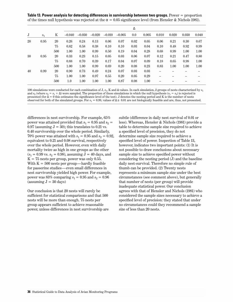
differences in nest survivorship. For example, 65%power was attained provided that s1 = 0.95 and s2 =0.97 (assuming J = 30); this translates to 0.21 vs.0.40 survivorship over the whole period. Similarly,70% power was attained with s1 = 0.95 and s2 = 0.92,equivalent to 0.21 and 0.08 survival, respectivelyover the whole period. However, even with dailymortality twice as high in one groups as the other (s1 = 0.99 vs. s2 = 0.98), assuming J = 40 days, andK = 75 nests per group, power was only 0.55. With K = 500 nests per group—hardly feasible for passerine studies—even small differences innest survivorship yielded high power. For example,power was 83% comparing s1 = 0.95 and s2 = 0.96(assuming J = 30 days)

Our conclusion is that 20 nests will rarely besufficient for statistical comparisons and that 500nests will be more than enough. 75 nests pergroup appears sufficient to achieve reasonablepower, unless differences in nest survivorship are

subtle (difference in daily nest survival of 0.01 orless). Whereas, Hensler & Nichols (1981) provide atable to determine sample size required to achievea specified level of precision, they do notdetermine sample size required to achieve aspecified level of power. Inspection of Table 13,however, indicates two important points: (1) It isnot possible to draw conclusions about necessarysample size to achieve specified power withoutconsidering the nesting period (J) and the baselinedaily nest-survival. Therefore no simple rule ofthumb can be provided. (2) Twenty nestsrepresents a minimum sample size under the bestcircumstances (see comment above), but generallythat number of nests (per group) will provideinadequate statistical power. Our conclusionagrees with that of Hensler and Nichols (1981) whoconsidered the sample sizes necessary to achieve aspecified level of precision: they stated that underno circumstances could they recommend a samplesize of less than 20 nests.


Table 13. Power analysis for detecting differences in survivorship between two groups. Power = proportionof the times null hypothesis was rejected at the α = 0.05 significance level (from Hensler & Nichols 1981).

∆

J s1 K –0.040 –0.030 –0.020 –0.010 –0.005 0.0 0.005 0.010 0.020 0.030 0.040

20 0.95 20 0.26 0.24 0.13 0.06 0.07 0.02 0.05 0.06 0.21 0.30 0.6775 0.82 0.58 0.38 0.10 0.10 0.03 0.04 0.10 0.48 0.92 0.99500 1.00 1.00 0.99 0.50 0.19 0.04 0.28 0.68 0.99 1.00 1.00

30 0.95 20 0.33 0.23 0.15 0.05 0.03 0.06 0.07 0.12 0.21 0.47 0.8075 0.88 0.70 0.39 0.17 0.04 0.07 0.09 0.18 0.65 0.98 1.00500 1.00 1.00 0.99 0.69 0.20 0.08 0.23 0.83 1.00 1.00 1.00

40 0.99 20 0.90 0.73 0.49 0.24 0.07 0.03 0.03 – – – –75 1.00 1.00 0.97 0.55 0.20 0.05 0.29 – – – –500 1.0 1.00 1.00 1.00 0.87 0.08 1.00 – – – –

100 simulations were conducted for each combination of J, s1, K and ∆ values. In each simulation, 2 groups of nests characterized by s1and s2 (where s2 = s1 + ∆) were sampled. The proportion of these simulations in which the null hypothesis (s1 = s2) is rejected ispresented (for ∆ = 0 this estimates the significance level of the test). J denotes the nesting period and K is the number of nestsobserved for both of the simulated groups. For s1 = 0.99, values of ∆ ≥ 0.01 are not biologically feasible and are, thus, not presented.

Like linear regression and ANOVA, logisticregression is a broadly applicable method, one thatis particularly suited for the analysis of binaryoutcomes; i.e., any situation in which the outcomecan be can be scored either “1” or “0” and theprobability of that outcome can be related to one ormore independent variables. We have already brieflymentioned it in regard to analysis of presence/absence data obtained from point counts. Anotherexample might be the analysis of environmentalfactors that relate to nest site selection, comparingsites with nests (scored 1) and sites without nests(scored 0). Survival of a nest to fledging is yetanother example where logistic regression might beapplied. Important features of logistic regressioninclude the following:

1. Like linear regression, the outcome variable inlogistic regression is modeled as a linearcombination of predictor or independent variables.However, an important distinction is that becausethe response variable is measured on a discrete,binary level, the error term has a binomialdistribution, not a normal distribution, as is foundwith linear regression. Linear regression estimatesthe mean of a dependent variable for a set ofpredictor values, while logistic regression estimatesthe proportion of responses in one of two possibleoutcomes given a set of predictor values.

2. Unlike linear regression, the outcome (e.g.,survived or died, scored 1 or 0, respectively) is firsttransformed before being analyzed. If p refers tothe probability of survival, then logistic regressionanalyzes the natural logarithm of [p/(1-p)].Therefore p/(1-p) can be thought of as the odds ofsurvival. For example, when the probability ofsurviving is 0.75, the odds of surviving = 0.75/0.25 or3, meaning that the odds of surviving are threetimes as great as the odds of dying. ln[p/(1-p)] isreferred to as logit p. In the case of simple logisticregression (analogous to simple linear regression),the relationship being modeled is:

logit p = a + bx,

where x is the independent variable, a is theintercept for the equation and b is the regressioncoefficient. This relationship can be rewritten as:

It is easy to see that the relationship between p andx will be non-linear, even though the relationshipbetween logit p and x is linear. One can use thelogistic equation to provide the expected orpredicted proportion of “successes” for a given xvalue.

3. Logistic regression makes no assumptions aboutthe independent variables, unlike discriminantanalysis (Kleinbaum et al. 1988, Ludwig & Reynolds1988), which assumes that the independent variablesare distributed as a multi-variate normal.

4. Logistic regression does, however, assumeindependence of outcome among all observations.Suppose we are following survival to fledglingamong 100 nestlings that came from 20 broods. Eachnestling is classified as having survived (scored 1) ordied (scored 0). Logistic regression on the fate of the100 nestlings would require that each nestlingsurvive or die independently of all others, includingits siblings. However, survival among siblings,especially while still in the nest, cannot be assumedto be independent but this assumption could betested. Linear regression based on 100 observationsmay also be inappropriate. However, here we cancollapse the data and analyze survival from 20broods; the outcome is a number between 0 and 5.Analysis of an outcome that takes on 6 differentvalues is not possible for standard logisticregression, in which the outcome must be 0 or 1.There are variants of logistic regression which canaccommodate non-independence of observations,e.g., available in EGRET, a user-friendly, menu-driven program with an excellent, easy-to-understand manual (available from S.E.R.C., 909Northeast 43rd St., Seattle, WA, 98105). Anothervariant on logistic regression is ordered logisticregression, which can be implemented in STATA(see address above).

ea+bxp = _________

1+ea+bx

37

V. Logistic Regression

Example 9: Analysis of Presence/Absence Data Using Logistic RegressionWe provide the following example of logisticregression, from a study of factors influencingabundance and distribution of GrasshopperSparrows (Ammodramus savannarum) and otherspecies on a shrub- steppe and grassland site ineastern Oregon (Holmes & Geupel 1998). Holmesand Geupel (1998) analyzed the presence or absenceof Grasshopper Sparrows at 220 point count stationsover a 3 year period in relation to a suite of habitatand vegetation features. Here we focus on data fromthe 141 point counts situated in shrub, in relation tothe influence of three habitat variables: perennialgrass cover, overall shrub cover, and density of bigsagebrush (Artemesia tridentata). Considered oneat a time, each is strongly associated with thepresence (in the case of perennial grass) or absence(in the case of shrub cover and Artemesiatridentata) of Grasshopper Sparrows. Annotatedstatistical results output from STATA from thesingle-variable logistic regression analyses arepresented in Table 14 (A, B, and C).

1. The likelihood ratio statistic (LRS), degrees offreedom (in parentheses), and associated P-value arepresented for the overall model. Under the nullhypothesis, the LRS is distributed as a chi-squaredstatistic, hence STATA labels the statistic “chi2(df).”However, because the LRS is a different statisticfrom the “usual” chi squared statistic (Pearsongoodness-of-fit), we prefer to label it LRS.

2. STATA presents a statistic “Pseudo R2” which iscomparable to R2 from ANOVA conducted onindividual observations. The interpretation ofPseudo R2 is the same as the usual R2: it is theproportion of variation in the dependent variableaccounted for by the independent variable orvariables. In this case, 31% of variation in presenceor absence of Grasshopper Sparrows at individualpoint count stations can be accounted for by anindex of perennial grass cover.

3. The log likelihood of the model is presented. Werefer the reader to texts such as Kleinbaum et al.(1988) for more extensive discussion of loglikelihood. For every statistical model a likelihoodcan be calculated which measures how well thatmodel accounts for the observed outcomes.Because the likelihood is a number less than 1, thelog likelihood is always negative. Thus, the morenegative the log likelihood, the more poorly doesthat model account for the observed variation inthe dependent variable. Comparing Table 14A and14C we see that the model with perennial grasscover accounts for more of the variation inGrasshopper Sparrow presence and absence than

does the model with Artemesia only: the formerhas a less negative log likelihood and, consequently,a greater Psuedo R2.

4. The logistic regression coefficient and its standarderror are shown. The results imply that an increasein the log(perennial grass cover) index of one unitincreases the logit(p) by +2.28 units, where p refersto the presence of Grasshopper Sparrows at thatpoint count station.

5. STATA provides a statistical test for thesignificance of each independent variable in themodel. This test is referred to as a Wald test.However, this test is not recommended (Hosmer andLemeshow 1989), because the nominal P-value doesnot correspond well to actual P-value. In some cases,the P-value from the Wald test is too high, leading toa Type II error. Instead, the Likelihood Ratio Testand its associated statistic, LRS, is recommendedfor statistical inference (Kleinbaum et al. 1988,Lebreton et al. 1992). Essentially, the Wald testprovides a quick and easy test of the P-value for anindependent variable. The problem is that using thisquick and easy estimate is often unreliable.

The relationship between Grasshopper Sparrowpresence and perennial grass cover is showngraphically in Figure 5, showing the predictedprobability of Grasshopper Sparrow presence (overthe course of the 3 year study), derived from thestatistical model in Table 14A. This shows (Figure 5)the actual percentages of occurrence of GrasshopperSparrows in relation to the perennial grass coverindex (PGCI) at each point count station. Thesepercentages of Grasshopper Sparrow occurrencewere obtained by grouping point count stations thathad similar PGCI values. An index value of 0 (whichcorresponds to 0% perennial grass cover) and theprobability of detecting one or more GrasshopperSparrows at that point count station over a 3 yearperiod was about 30%. The probability of detecting aGrasshopper Sparrow increased to 40 to 50% with asmall increase in the PGCI to a value of 0.5. With aPGCI value of 1 (corresponding to a perennial grasscover of 1%), the probability of detecting aGrasshopper Sparrow increases to over 70%. With aPGCI value of 1.5 (corresponding to a perennialgrass cover of 3%), the probability of detecting aGrasshopper exceeds 90%. And by the time thePGCI reaches 2.0 (corresponding to a perennialgrass cover of over 5%), the probability of detectinga Grasshopper Sparrow at that point count stationapproaches 100%.

Having obtained the results in Table 14 A, B, and C,the investigator may wish to conduct a multiplelogistic regression analysis to determine how manydifferent factors may be contributing to variation in


Logistic Regression 39

Table 14. Logistic regression analysis of Grasshopper Sparrow presence/absence in relation to habitatfeatures (from Holmes & Geupel 1998). Dependent variable is detection of Grasshopper Sparrow at any of 9surveys (scored as “1”), conducted at 141 point count stations. A. Simple logistic regression in relation toPerennial Grass. B. Simple logistic regression in relation to shrub cover. C. Simple logistic regression inrelation to Artemesia Density. D. Multiple logistic regression analysis with all 3 independent variables.E. Best, multiple logistic regression model, and associated goodness-of-fit statistics.

A) Independent Variable: Perennial Grass Cover Index [lpergras] = ln(Perennial Grass Cover + 1), where Perennial Grass Cover is measured on 0 to 100 scaleLogit Estimates Number of obs = 141

chi2(1) = 60.23Prob >chi2 = 0.0000

Log Likelihood = –67.584999 Pseudo R2 = 0.3083Coef. Std. Err. z P>|z| [95% Conf. Interval]

lpergras 2.280344 .486312 4.689 0.000 1.32719 3.233499

B) Independent Variable: Shrub Cover [shrubcov] (on 0 to 100 scale)Logit Estimates Number of obs = 141

chi2(1) = 22.02Prob >chi2 = 0.0000


shrubcov –.0778626 .0182709 –4.262 0.000 –.113673 –.0420522

C) Independent Variable: Density of Artemesia [artemden] = number of individualsLogit Estimates Number of obs = 141

chi2(1) = 15.09Prob >chi2 = 0.0001


artemden –.0200667 .0055873 –3.591 0.000 –.0310177 –.0091157

D) Multiple logistic regression analysis with all 3 independent variablesLogit Estimates Number of obs = 141

chi2(3) = 74.26Prob >chi2 = 0.0000


lpergras 2.797955 .7079792 3.952 0.000 1.410342 4.185569shrubcov –.0215319 .0252564 –0.853 0.394 –.0710336 .0279697artemden –.0198948 .0081006 –2.456 0.014 –.0357716 –.004018_cons –.1434713 .496225 –0.289 0.772 –1.116054 .8291118

Likelihood Ratio Test for each independent variable while controlling for the other two:lpergras LRS = 50.37, df=1, P <0.0001shrubcov LRS = 0.74, df=1, P = 0.39artemden LRS = 6.50, df=1, P =0.011

E) Best multiple logistic regression modelLogit Estimates Number of obs = 141

chi2(2) = 73.53Prob >chi2 = 0.0000


lpergras 2.846168 .7031315 4.048 0.000 1.468056 4.224281artemden –.0231516 .0070722 –3.274 0.001 –.0370129 –.0092903_cons –.4889746 .2930915 –1.668 0.095 –1.063423 .0854741

Likelihood Ratio Test for each independent variable while controlling for the other:lpergras LRS = 58.43, df=1, P <0.0001artemden LRS = 13.29, df=1, P <0.001

Hosmer-Lemeshow Goodness of Fit test for above model:number of observations = 141number of groups = 15Hosmer-Lemeshow chi2(13) = 6.21Prob >chi2 = 0.938

{③

④ ⑤①

②

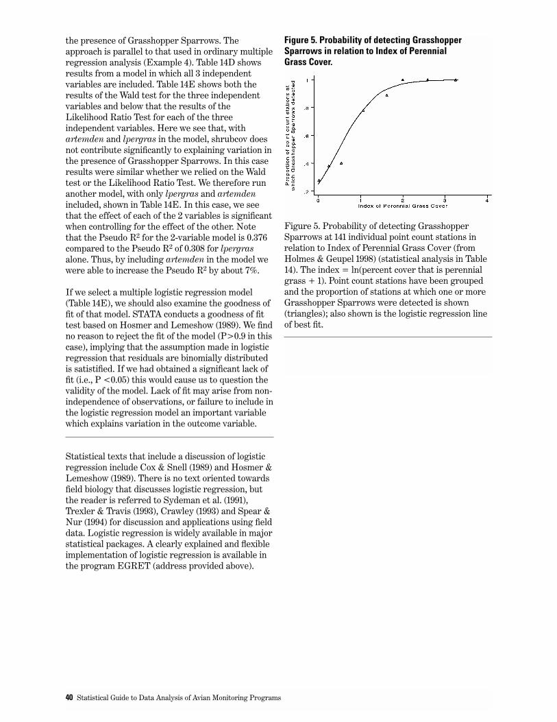
the presence of Grasshopper Sparrows. Theapproach is parallel to that used in ordinary multipleregression analysis (Example 4). Table 14D showsresults from a model in which all 3 independentvariables are included. Table 14E shows both theresults of the Wald test for the three independentvariables and below that the results of theLikelihood Ratio Test for each of the threeindependent variables. Here we see that, withartemden and lpergras in the model, shrubcov doesnot contribute significantly to explaining variation inthe presence of Grasshopper Sparrows. In this caseresults were similar whether we relied on the Waldtest or the Likelihood Ratio Test. We therefore runanother model, with only lpergras and artemdenincluded, shown in Table 14E. In this case, we seethat the effect of each of the 2 variables is significantwhen controlling for the effect of the other. Notethat the Pseudo R2 for the 2-variable model is 0.376compared to the Pseudo R2 of 0.308 for lpergrasalone. Thus, by including artemden in the model wewere able to increase the Pseudo R2 by about 7%.

If we select a multiple logistic regression model(Table 14E), we should also examine the goodness offit of that model. STATA conducts a goodness of fittest based on Hosmer and Lemeshow (1989). We findno reason to reject the fit of the model (P>0.9 in thiscase), implying that the assumption made in logisticregression that residuals are binomially distributedis satistified. If we had obtained a significant lack offit (i.e., P <0.05) this would cause us to question thevalidity of the model. Lack of fit may arise from non-independence of observations, or failure to include inthe logistic regression model an important variablewhich explains variation in the outcome variable.

Statistical texts that include a discussion of logisticregression include Cox & Snell (1989) and Hosmer &Lemeshow (1989). There is no text oriented towardsfield biology that discusses logistic regression, butthe reader is referred to Sydeman et al. (1991),Trexler & Travis (1993), Crawley (1993) and Spear &Nur (1994) for discussion and applications using fielddata. Logistic regression is widely available in majorstatistical packages. A clearly explained and flexibleimplementation of logistic regression is available inthe program EGRET (address provided above).


Figure 5. Probability of detecting GrasshopperSparrows at 141 individual point count stations inrelation to Index of Perennial Grass Cover (fromHolmes & Geupel 1998) (statistical analysis in Table14). The index = ln(percent cover that is perennialgrass + 1). Point count stations have been groupedand the proportion of stations at which one or moreGrasshopper Sparrows were detected is shown(triangles); also shown is the logistic regression lineof best fit.

Figure 5. Probability of detecting GrasshopperSparrows in relation to Index of Perennial Grass Cover.

We conceived of this Statistical Guide as a jumping-off point for biologists wishing to design and analyzedata from population monitoring programs. Werecognize that we have presented less detail on somepoints or areas than some readers would like, andtherefore have recommended texts, or otherreferences, that consider more specialized topics ingreater detail. Our objective has been to provideguideposts, not to provide an encyclopedictreatment of statistical analysis and design.Statistical analysis is a field that progresses rapidly,and thus analytic methods that were recommendeda decade or two ago have now been superseded. Weexpect that methods that are only now beingconsidered (e.g., application of time-to-failureanalyses) will be commonplace in a few years. Otheranalytic methods which interested readers shouldconsider, but which we have devoted little space to,include: bootstrapping and other re-samplingmethods, Poisson regression analysis, generalizedlinear models, and distance-sampling.

Computer programs evolve even faster than analyticmethods, and we have tried to provide currentinformation, but recognize that such informationbecomes obsolete very quickly. For this reason, werecognize that a Guide such as this is most usefulwhen it remains current. Therefore, we encouragereaders to send comments and corrections to thesenior author, so as to improve the quality of thenext versions.

41

VI. Concluding Remarks

Anderson-Sprecher, R. 1994. Model comparisons andR2. Am. Statistician 48:113-117.

Arnason, A.N. and C.J. Schwarz. 1986. POPAN-3:extended analysis and testing features forPOPAN-2. Charles Babbage Research Centre,St. Pierre, Manitoba, Canada.

Baicich, P.J. and C.J.O. Harrison. 1997. A guide tothe nests, eggs, and nestlings of North America, 2nded. Academic Press, San Diego, CA.

Bart, J. and W. Notz. 1996. Analysis of data. In T.A.Bookhout (ed.), Research and managementtechniques for wildlife and habitats, 5th ed. TheWildl. Soc., Bethesda, MD.

Bart, J., M. Fligner, and W. Notz. 1998. Samplingand statistical methods for behavioral ecologists.Cambridge Univ. Press, England.

Bibby, C.J., N.D. Burgess, and D.A. Hill. 1992. Birdcensus techniques. Academic Press, London,England.

Bromaghin, J.F. and L.L. McDonald. 1993. Asystematic-encounter-sampling design for nestingstudies. Auk 110:646-651.

Brownie, C., D.R. Anderson, K.P. Burnham, and D.S.Robson. 1985. Statistical inference from bandrecovery data-a handbook. U.S. DOI Fish & Wildl.Serv., Resource Publi. 156.

Buckland, S.T. 1980. A modified analysis of the Jolly-Seber capture-recapture model. Biometrics 36:419-435.

Buckland, S.T., D.R. Anderson, K.P. Burnham, andJ.L. Laake. 1993. Distance sampling: estimatingabundance of biological populations. Chapman &Hall, London, England.

Burnham, K.P., D.R. Anderson, G.C. White, C.Brownie, and K.H. Pollock. 1987. Design andanalysis methods for fish survival experimentsbased on release-recapture. Am. Fisheries Soc.Monogr. 5.

Butcher, G.S. 1992. Needs Assessment: monitoringneotropical migratory birds. Unpubl. report forPartners in Flight, Ithaca, NY.

Chase, M., N. Nur, and G. R. Geupel. 1997. Survival,productivity, and abundance of a Wilson’s Warblerpopulation. Auk 114:354-366.

Cohen, J. 1988. Statistical power analysis for thebehavioral sciences, 2nd ed. Lawrence ErlbaumAssociates, Hillsdale, NJ.

Clobert, J., J.D. Lebreton and D. Allainé. 1987. Ageneral approach to survival rate estimation byrecaptures or resightings of marked birds. Ardea75:133-42.

Cooch, E., R. Pradel, and N. Nur. 1996. A practicalguide to mark-recapture analysis using SURGE.Centre d’Ecologie Fonctionelle et Evolutive, CNRS,Montpellier, France.

Cox, D.R. and D. Oakes. 1984. Analysis of survivaldata. Chapman and Hall, London, England.

Cox, D.R. and E.J. Snell. 1989. Analysis of binarydata. Chapman and Hall, London, England.

Crawley, M.J. 1993. GLIM for ecologists. BlackwellScientific, Oxford, England.

Dawson, D.G. 1981. Experimental design whencounting birds. In C. J. Ralph and J. M. Scott (eds.),Estimating numbers of terrestrial birds. Stud. inAvian Biol. No. 6.

DeSante, D.F, K.M. Burton, and O.E. Williams. 1993.The monitoring avian productivity and survivorship(MAPS) program second annual report. BirdPopulations 1:1- 28.

DeSante, D.F., and G.R. Geupel. 1987. Landbirdproductivity in central coastal California: therelationship to annual rainfall and a reproductivefailure in 1986. Condor 89:636-653.

Dieni, J.S. 1996. The effects of burning on breedingbird community structure in aspen forests. Ms.Thesis, Univ. of Wyoming, Laramie.

42

References

Draper, N.R. and H. Smith. 1981. Applied regressionanalysis, 2nd ed. John Wiley, NY.

Ellison, A.M. 1992. Statistics for PCs. Bull. Ecol.Soc. of Am. 73:74-87.

Erdfelder, E., F. Faul, and A. Buchner. 1996.GPOWER: a general power analysis program.Behaviour Research Methods, Instruments, andComputers 28:1-11.

Fleiss, J. L. 1981. Statistical methods for rates andproportions, 2d ed. Wiley & Sons, NY.

Gerrodette, T. 1987. A power analysis for detectingtrends. Ecology 68:1364-1372.

Gerrodette, T. 1991. Models of power of detectingtrends—a reply to Link and Hatfield. Ecology72:1889-1892.

Geupel, G.R. and D.F. DeSante, 1990. Incidence anddeterminants of double brooding in Wrentits.Condor 92:67-75.

Geupel, G.R. and I. Warkentin. 1995. Field methodsfor monitoring population parameters of landbirdsin Mexico. In M. Wilson and S. Saeder (eds.),Conservation of neotropical migrant birds inMexico. Maine Agricult. and For. Experiment Stat.Misc. Publi. 727, Orono, ME.

Göttmark, F. 1992. The effects of investigatordisturbance on nesting birds. Current Ornithol.9:63-104.

Greenwood, J.J.D. 1996. Basic techniques. In W.J.Sutherland (ed.), Ecological census techniques.Cambridge Univ. Press, England.

Gutzwiller, K.J. and H.A. Marcum. 1997. Birdreactions to observer clothing color: implications fordistance-sampling techniques. J. Wildl. Manage.61:935-947.

Hays, R.L., C. Summers, and W. Seitz. 1981.Estimating wildlife habitat variables. U.S. DOI, Fish& Wildl. Serv., FWS/OBS-8147, Washington, D.C.

Hensler, G.L. and J.D. Nichols. 1981. The Mayfieldmethod of estimating nesting success: a model,estimators and simulation results. Wilson Bull.93:42-53.

Hicks, C.R. 1982. Fundamental concepts in thedesign of experiments, 3rd ed. Holt, Rinehart andWinston, NY.

Holmes, A. and G.R. Geupel. 1998. Avian populationstudies at the Naval Weapons Systems TrainingFacility, Boardman, Oregon. Unpubl. final report ofthe Point Reyes Bird Observatory to U.S. Navy andOregon Department of Fish & Game. (Availablefrom PRBO, 4990 Shoreline Highway, StinsonBeach, CA 94970.)

Hosmer, D.W. and S. Lemeshow. 1989. Appliedlogistic regression. Wiley & Sons, NY.

Hurlbert, S.H. 1984. Pseudoreplication and thedesign of ecological field experiments. Ecol. Monogr.54:187-211.

Hutto, R.L., S.M. Pletscet, and P. Hendricks. 1986. Afixed- radius point count method for nonbreedingand breeding season use. Auk 103:593-602.

Hutto, R.L. and C. Paige, 1995. USDA ForestService Northern Region landbird monitoringprogram. Unpubl. report of USDA For. Serv.(Available from Div. of Biological Science. Universityof Montana, Missoula, MT 59812.)

James, F.C. and H.H. Shugart, Jr. 1970.A quantitative method of habitat description.Audubon Field Notes 24:727-736.

Johnson, D.H. In Press. Statistical considerations in monitoring birds over large areas. In Bonney, R.,D. N. Pashley, R. Cooper and L. Niles (eds.).Strategies for Bird Conservation: The Partners in Flight Planning Process. Proceedings of the1995 Cape May International Partners in FlightWorkshop. Cornell Lab of Ornithology.<http://birds.cornell.edu/pifcapemay> (Availablefrom D. H. Johnson, NPWRC, USGS-BRD,Jamestown, ND 58401.)

Johnson, D.H. 1979. Estimating nest success: theMayfield method and an alternative. Auk 96:651-661.

Johnson, M.D. and G.R. Geupel. 1996. Theimportance of productivity to the dynamics of aSwainson’s Thrush population. Condor 98:133-141.

Kalbfleisch, J.D. and R.L. Prentice. 1980. Thestatistical analysis of time to failure data. JohnWiley, NY.

Kleinbaum, D.G., L.L. Kupper, and K.E. Muller.1988. Applied regression analysis and othermultivariable methods, 2nd ed. PWS-Kent Pub. Co.,Boston, MA.

References 43

Knopf, F.L., J.A. Sedgwick, and R.W. Cannon. 1988.Guild structure of a riparian avifauna relative toseasonal cattle grazing. J. Wildl. Manage. 51:280-290.

Krebs, C. 1989. Ecological methodology. Harper andRow, NY.

Laake, J.L., S.T. Buckland, D.R. Anderson, and K.PBurnham, 1993. DISTANCE User’s Guide. ColoradoCooperative Fish & Wildl. Research Unit, Col. StateUniv., Fort Collins, CO 80523.

Lancia, R.A., J.D. Nichols, and K.H. Pollock. 1996.Estimating the number of animals in wildlifepopulations. In T.A. Bookhout (ed.), Research andmanagement techniques for wildlife and habitats,5th ed. The Wildl. Soc., Bethesda, MD.

Larson, D.L. and C.E. Bock. 1986. Determiningavian habitat preference by bird-centeredvegetation sampling. In J. Verner, C.J. Ralph, andM.L. Morrison (eds.), Wildlife 2000: Modelinghabitat relationships of terrestrial vertebrates. Univ.of Wisconsin Press, Madison, WI.

Lebreton, J.-D., K.P. Burnham, J. Clobert, and D.R.Anderson. 1992. Modeling survival and testingbiological hypotheses using marked animals: aunified approach with case studies. Ecol. Monogr.62:67-118.

Lebreton, J.-D., A.-M. Reboulet, and G. Banco. 1993.An overview of software for terrestrial vertebratepopulation dynamics. In J.-D. Lebreton, and P.M.North (eds.), Marked individuals in the study of birdpopulations. Birkhaeuser Verlag, Basel, Germany.

Link, W.A. and J.S. Hatfield. 1990.Power calculations and model selection for trendanalysis: a comment. Ecology 71:1217-1220.

Lokemoen, J. and R. Koford. 1996. Using candlers todetermine the incubation stage of passerine eggs. J.Field Ornithol. 67:660-668.

Loyn, R.H. 1986. The 20 minute search—a simplemethod for counting forest birds. Corella 10:58-60.

Ludwig, J.A. and J.F. Reynolds. 1988. StatisticalEcology: a primer on methods and computing. Wiley& Sons, NY.

MacArthur, R.H. 1965. Patterns of species diversity.Biol. Rev. 40:510-533.

Magurran, A.E. 1988. Ecological diversity and itsmeasurement. Princeton Univ. Press, NJ.

Martin, T.E. 1992. Breeding productivityconsiderations: what are the appropriate habitatfeatures for management? In J. M. Hagan and D. W.Johnston (eds.), Ecology and conservation ofneotropical migrant birds. Smithson. Inst. Press,Washington, D.C.

Martin, T.E. and P. Li. 1992. Life history traits ofopen- vs. cavity-nesting birds. Ecology 73:579-592.

Martin, T.E. and G.R. Geupel. 1993. Nest monitoringplots: methods for locating nests and monitoringsuccess. J. Field. Ornithol. 64:507-519.

Martin, T.E. and J.J. Roper. 1988. Nest predationand nest site selection of a western population of theHermit Thrush. Condor 90:51-57.

Martin, T.E., J. Clobert, and D.R. Anderson. 1995.Return rates in studies of life history evolution: arebiases large? J. Appl. Statistics 22:863-875.

Martin, T.E., C. Paine, C.J. Conway, W.M.Hochachka, P. Allen, and W. Jenkins. 1997. BBIRDField Protocol. (Document available from MontanaCooperative Wildlife Research Unit, Univ. ofMontana, Missoula, MT 59812; web site: http://pica.wru.umt.edu/bbird/)

Mayfield, H. 1961. Nesting success calculated fromexposure. Wilson Bull. 73:255-261.

Mayfield, H. 1975. Suggestions for calculating nestsuccess. Wilson Bull. 87:456-466.

McShea, W.J. and J.H. Rappole. 1997. Variable songrates in three species of passerines and implicationsfor estimating bird populations. J. Field Ornithol.68:367-375.

Neter, J., W. Wasserman and M.H. Kutner. 1990.Applied linear statistical models: regression,analysis of variance, and experimental designs, 3rdedition. Irwin, Homewood, Ill.

Noon, B.R. 1981. Techniques for sampling avianhabitat. In D.E. Capen (ed.), The use of multivariatestatistics in studies of wildlife habitat. USDA For.Serv., GTR-RM-87, Rocky Mountain Forest andRange Station, Fort Collins, CO.

Nur, N. and J. Clobert. 1988. Measuring Darwinianfitness in birds: a field guide. In H. Ouellet (ed.),Acta XIX Congressus Internationalis Ornithologici.Univ. of Ottawa Press, Canada.


Nur, N. and G.R. Geupel. 1993a. Validating the use ofconstant effort mist-netting to monitor avianpopulations. Unpubl. PRBO final report to U.S. Fish& Wildl. Serv. (Available from Point Reyes BirdObservatory, Stinson Beach, CA 94970).

Nur, N. and G.R. Geupel. 1993b. Evaluation of nestmonitoring, mist-netting, and other methods formonitoring demographic processes in landbirdpopulations. In D. M. Finch and P. W. Stangel (eds.),Status and management of neotropical migrantbirds. USDA For. Serv. Publ.: GTR RM-229, FortCollins, CO.

Nur, N., G.R. Geupel, and G. Ballard. 1994.Assessing the impact of the Cantara spill onterrestrial bird populations along the SacramentoRiver: Results from the 1993 field season. Unpubl.report to California Dept. of Fish and Game.(Available from Point Reyes Bird Observatory,Stinson Beach, CA 94970).

Ortega, C.P., J.C. Ortega, C.A. Rapp, S. Vorisek, S.A.Backensto, and D.W. Palmer. 1997. Effect of researchactivity on the success of American Robin nests. J.Wildl. Manage. 61:948-952.

Peach, W.J., S.R. Baillie, and L. Underhill. 1991.Survival of British Sedge Warblers Acrocephalusschoenobaenus in relation to west African rainfall.Ibis 133:300-305.

Peach, W.J. 1993. Combining mark-recapture datasets for small passerines. In J.-D. Lebreton and P.M. North (eds.), Marked individuals in the study ofbird populations. Birkhaeuser, Basel, Germany.

Pielou, E. C. 1975. Ecological diversity. Wiley, NewYork.

Pollock, K.H., and W.L. Cornelius. 1988. Adistribution-free nest survival model. Biometrics44:397-404.

Pollock, K.H., J.D. Nichols, C. Brownie, and J.E.Hines. 1990. Statistical inference for capture-recapture experiments. Wildl. Monogr. 107.

Pradel, R. and J.-D. Lebreton. 1993. User’s manualfor program SURGE Version 4.2. CEFE/CNRS,Montpelier. (Available from J.-D. Lebreton, CEFE/CNRS, BP 5051, 34033 Montpellier Cedex, France.)

Ralph, C.J., G.R. Geupel, P. Pyle, T.E. Martin, andD.F. DeSante. 1993. Handbook of field methods formonitoring landbirds. USDA For. Serv. Publ., PSW-GTR-144, Albany, CA.

Ralph, C.J., S. Droege, and J.R. Sauer. 1995.Monitoring bird populations by point counts. USDAFor. Serv. Publ., Gen. Tech. Rep. PSW-GTR-149,Albany, CA.

Ralph, C.J. and J.M. Scott. 1981. Estimatingnumbers of terrestrial birds. Stud. in Avian Biol.,No. 6.

Ramsey, F.L. and J. M. Scott. 1981. Analysis of birdsurvey data using a modification of Emlen’s method.In C. J. Ralph and J. M. Scott (eds.), Estimatingnumbers of terrestrial birds. Stud. in Avian Biol.,No. 6.

Robinson, S.K., F.R. Thompson, T.M. Donovan, D.R.Whitehead, and J. Faaborg. 1995. Regional forestfragmentation and the nesting success of migratorybirds. Science 267:1987-1990.

Sauer, J.R. 1998. Inventory methods for birds.Unpublished report to U.S. DOI National Park Serv.

Sauer, J.R. and B.K. Williams. 1989. Generalizedprocedures for testing hypotheses about survival orrecovery rates. J. of Wildl. Manage. 53:137-142.

Skalski, J.R. and D.S. Robson. 1992. Techniques forwildlife investigations: Design and analysis ofcapture data. Academic Press, San Diego, CA.

Sherry, T. and R. Holmes. 1993. Are populations ofneotropical migrant birds limited in summer ofwinter? In D. M. Finch and P. W. Stangel (eds.),Status and management of neotropical migrantbirds. USDA For. Serv. Publ.: GTR RM-229, FortCollins, CO.

Silkey, M., N. Nur and G.R. Geupel. 1999. Can mistnets track annual variation in abundance? Avalidation study. Condor.

Slater, P.J. 1994. Factors affecting the efficiency ofthe area search method of censusing birds in openforests and woodlands. Emu 94:9-16.

Snedecor, G.W. and W.G. Cochran. 1989. Statisticalmethods, 8th edition. Iowa State Univ. Press, Ames.

Spear, L. and N. Nur. 1994. Brood size, hatchingorder and hatching date: effects on four life-historystages from hatching to recruitment in westerngulls. J. of Animal Ecol. 63:283-298.

Sokal, R.R. and F.J. Rohlf. 1995. Biometry: theprinciples and practice of statistics in biologicalresearch, 3rd ed. W. H. Freeman, San Francisco, CA

References 45

StataCorp. 1999. Stata Statistical Software, Release6.0. Stata Corporation, College Station, TX.

Sydeman, W.J., H.R. Huber, S.D. Emslie, C.A. Ribic,and N. Nur. 1991. Age-specific weaning success ofNorthern elephant seals in relation to previousbreeding experience. Ecology 72:2204-2217.

Thomas, L. and C.J. Krebs. 1997. A review ofstatistical power analysis software. Bull. Ecol. Soc.of Am. 78:126-138.

Thomas, L. 1996. Monitoring long-term populationchange: why are there so many analysis methods?Ecology 71:49-58.

Trexler, J.C. and J. Travis. 1993. Nontraditionalregression analyses. Ecology 74:1629-1637.

Verner, J. 1985. Assessment of counting techniques.Current Ornithol. 2:247-301.

Verner, J. and T. A. Larson. 1989. Richness ofbreeding bird species in mixed-conifer forest of theSierra Nevada, CA. Auk 106:447-461.

White, G.C. 1986. Program SURVIV user’s manual,version 1.2. Dept. of Fishery and Wild. Biol.,Colorado State Univ., Fort Collins.

White, G.C., D.R. Anderson, K.P. Burnham, andD.L. Otis. 1982. Capture-recapture and removalmethod for sampling closed population. Los AlamosNational Laboratory, LA-8787-NERP.

Zar, J.H. 1996. Biostatistical analysis, 3rd ed.Prentice-Hall, Inc., Englewood Cliffs, NJ


47

Notes and Calculations

Notes and Calculations 49

U.S. Department of the InteriorU.S. Fish & Wildlife Service

http://www.fws.gov

Statistical Guide to Data Analysis of Avian Monitoring ... · Statistical Guide to Data Analysis of...

Documents

Transcript of Statistical Guide to Data Analysis of Avian Monitoring ... · Statistical Guide to Data Analysis of...