Statistical Evolutionary Laws in Music Styles

Eita Nakamura1∗ and Kunihiko Kaneko2†

1 The Hakubi Center for Advanced Research and Graduate School of Informatics,

Kyoto University, Sakyo, Kyoto 606-8501, Japan

2 Center for Complex Systems Biology, Universal Biology Institute, University of Tokyo,

Meguro, Tokyo 153-8902, Japan

If a cultural feature is transmitted over generations and exposed to stochas-

tic selection when spreading in a population, its evolution may be governed by

statistical laws and be partly predictable, as in the case of genetic evolution.

Music exhibits steady changes of styles over time, with new characteristics de-

veloping from traditions. Recent studies have found trends in the evolution of

music styles, but little is known about their relations to the evolution theory.

Here we analyze Western classical music data and find statistical evolutionary

laws. For example, distributions of the frequencies of some rare musical events

(e.g. dissonant intervals) exhibit steady increase in the mean and standard de-

viation as well as constancy of their ratio. We then study an evolutionary

model where creators learn their data-generation models from past data and

generate new data that will be socially selected by evaluators according to the

content dissimilarity (novelty) and style conformity (typicality) with respect

to the past data. The model reproduces the observed statistical laws and can

make non-trivial predictions for the evolution of independent musical features.

In addition, the same model with different parameterization can predict the

evolution of Japanese enka music, which is developed in a different society and

has a qualitatively different tendency of evolution. Our results suggest that the

evolution of musical styles can partly be explained and predicted by the evo-

lutionary model incorporating statistical learning, which can be important for

other cultures and future music technologies.

∗Electronic address: eita.nakamura@i.kyoto-u.ac.jp†Electronic address: kaneko@complex.c.u-tokyo.ac.jp

1

arX

iv:1

809.

0583

2v2

[ph

ysic

s.so

c-ph

] 5

Nov

201

9

Introduction

A prominent feature of humans is that they learn and transmit cultural traits over gen-

erations [1]. Although many cultural traits (e.g. style of music/language/fine art, fashion,

unscientific beliefs, etc.) seem to make little direct contribution to an individual’s biological

fitness, some of them (e.g. music and fashion) have evolved into highly complex forms and

have rather large influence on human behaviour. To understand human’s behaviour, it is

important to uncover some possible laws in cultural evolution and seek for a theory that

can explain them [2,3]. Moreover, a theory that can quantitatively predict parts of cultural

evolution can serve as a base for the development of new technologies to predict cultural

trend and enhance cultural production.

In this study, we consider the evolution of musical styles, which has gathered growing

attention [4–10]. It has been observed in a recent paper [11] that some features of music,

e.g. the frequency of tritones, have steadily increased during the history of Western classical

music. (The tritone is a pitch interval consisting of six semitones. It is regarded as a

“dissonant” interval in traditional music theories [12].) Although these clear trends imply

some driving force for the evolution of the music style, their theoretical origins and how much

they can be predicted are not understood. Moreover, while previous studies [4–6, 11] have

focused on the mean of musical features, other statistics including the standard deviation

and distribution form are important for studying their dynamics in relation to evolutionary

models [13].

Data Analysis

We first analyze the time evolution of statistics of musical features of Western classical

music data. In particular, we study two major aspects of tonal content of music, dissonance

and tonality, on which musicologists have focused [14, 15]. More specifically, we focus on

the frequencies of two features that represent these aspects and can be computationally

analyzed without interpretation of data by human. One of them is tritone, which is a

representative interval historically considered dissonant [14] and has been studied also in a

previous study [11] (see Refs. [16,17] for psychological studies on consonance and dissonance

of musical sound). The other one is non-diatonic motion, which is defined as bigrams of

pitch-class intervals that cannot be realized on a diatonic scale. (The C-major scale or

“the scale of white keys” (C-D-E-F-G-A-B) is one instance of diatonic scales. In general,

a diatonic scale can be transposed to the C-major scale by a global pitch shift.) The non-

diatonic motion is an indicator of chromatic motions and modulations (key changes) to a

distant key [18] (see Methods for a detailed definition).

Fig. 1(a) shows that the mean and standard deviation of the frequency (probability)

of tritones steadily increased during the years 1500–1900 while their ratio stayed approxi-

2

0.00001

0.00010

0.00100

0.01000

0.10000

1500s 1600s 1700s 1800s

Pro

babi

lity

Year

(a)

(b)

(c)

0

0.1

0.2

0 0.05 0.1 0.15

Nor

mal

ized

freq

uenc

y

Probability (frequency) Beta distribution fitting

1500s1600s1700s1800s

1500s 1600s

1700s 1800s

0

0.05

0.1

0.15

1500 1600 1700 1800 1900

Fre

quen

cy o

f trit

ones

Birth year of composer

0

0.5

1

1500 1600 1700 1800 1900(Std

. dev

.)/m

ean

Year

RenaissanceBaroque

Classical

Romantique

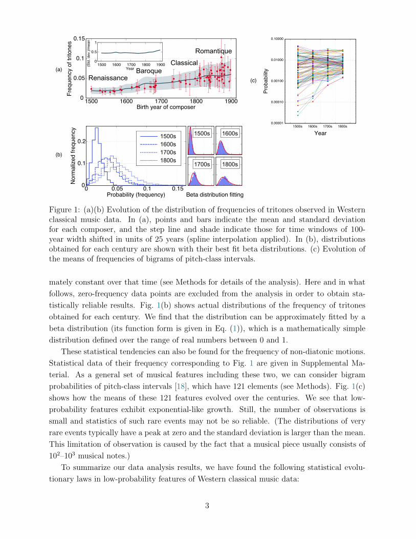
Figure 1: (a)(b) Evolution of the distribution of frequencies of tritones observed in Westernclassical music data. In (a), points and bars indicate the mean and standard deviationfor each composer, and the step line and shade indicate those for time windows of 100-year width shifted in units of 25 years (spline interpolation applied). In (b), distributionsobtained for each century are shown with their best fit beta distributions. (c) Evolution ofthe means of frequencies of bigrams of pitch-class intervals.

mately constant over that time (see Methods for details of the analysis). Here and in what

follows, zero-frequency data points are excluded from the analysis in order to obtain sta-

tistically reliable results. Fig. 1(b) shows actual distributions of the frequency of tritones

obtained for each century. We find that the distribution can be approximately fitted by a

beta distribution (its function form is given in Eq. (1)), which is a mathematically simple

distribution defined over the range of real numbers between 0 and 1.

These statistical tendencies can also be found for the frequency of non-diatonic motions.

Statistical data of their frequency corresponding to Fig. 1 are given in Supplemental Ma-

terial. As a general set of musical features including these two, we can consider bigram

probabilities of pitch-class intervals [18], which have 121 elements (see Methods). Fig. 1(c)

shows how the means of these 121 features evolved over the centuries. We see that low-

probability features exhibit exponential-like growth. Still, the number of observations is

small and statistics of such rare events may not be so reliable. (The distributions of very

rare events typically have a peak at zero and the standard deviation is larger than the mean.

This limitation of observation is caused by the fact that a musical piece usually consists of

102–103 musical notes.)

To summarize our data analysis results, we have found the following statistical evolu-

tionary laws in low-probability features of Western classical music data:

3

1. Beta-like distribution of frequency features

2. Steady increase of the mean and standard deviation

3. Nearly constant ratio of the mean and standard deviation, which is slightly less than

unity

4. (Possibly) exponential-like growth of the mean

These findings reveal that the evolution of styles in the classical music data exhibits much

more regularities than previously found [11]. The last two laws indicate that the dynamics

is scale invariant, that is, the dynamics at one value of the features looks similar to that at

a different value of the features. Since these statistical laws are found in the music data of

various composers in four consecutive centuries, they may be caused by general mechanisms

of transmission and selection of cultural style rather than by the circumstances of individual

composers or social communities of individual time periods.

Theoretical Model

Let us now discuss a possible evolutionary model that may explain the origin of the observed

statistical laws. Following the general framework of Darwinian evolution, we construct a

theoretical model based on information transmission and stochastic selection. A feature

of music culture is that creation styles are learned and transmitted via data (e.g. musical

scores and audio signals), and recent studies have suggested the importance of statistical

learning for music composition (e.g. [19–21]) and for lister’s understanding (e.g. [22]). As

is commonly done in the field of music informatics (e.g. [20, 21]), we represent creators

(composers) with statistical models for data generation and try to capture the evolution

of music styles through dynamic changes of creators’ models. As a driving force for time

evolution, we consider social selection by contemporary evaluators (listeners). Specifically,

we study a dynamical system of creators that statistically learn their data-generation models

from past data and then generate new data, and of evaluators that determine the fitness of

the generated data. Since evaluators should also learn their data-evaluation models from

existing data, it is legitimate to consider a dynamic change in the fitness depending on other

agents/data, as in evolutionary game theory [23]. Similar models of iterated learning have

been studied in the context of language evolution [24–26].

A dynamical system we call a statistical creator-evaluator (SCE) model is formulated as

follows. Each creator at generation t generates a dataset Xt of musical pieces according to

a distribution (data-generation model) φt, and the generated data are evaluated with the

fitness defined below. Following this evaluation, the creator’s model of the next generation

φt+1 is determined by statistical learning. With this procedure, the creator’s data-generation

model evolves over generations. The creator’s model φt(θ) is defined over a probability

parameter θ ∈ (0, 1) (e.g. frequency of some musical events). An evaluator is similarly

4

θ

θ

Generate LearnSelectionbased on

Creator’s model

Created data

φt(θ)

φt+1(θ)φt+2(θ)

θ

Evaluator’s modelψt(θ)

ψt+1(θ)ψt+2(θ)

Rt

Training data

Evaluate Learn

Xt = φt

Yt = φt

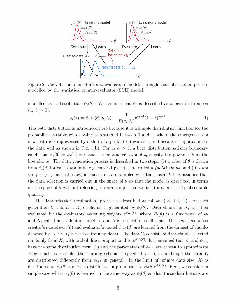
Figure 2: Coevolution of creator’s and evaluator’s models through a social selection processmodelled by the statistical creator-evaluator (SCE) model.

modelled by a distribution ψt(θ). We assume that φt is described as a beta distribution

(at, bt > 0):

φt(θ) = Beta(θ; at, bt) ≡1

B(at, bt)θat−1(1− θ)bt−1, (1)

The beta distribution is introduced here because it is a simple distribution function for the

probability variable whose value is restricted between 0 and 1, where the emergence of a

new feature is represented by a shift of a peak at 0 towards 1, and because it approximates

the data well as shown in Fig. 1(b). For at, bt > 1, a beta distribution satisfies boundary

conditions φt(0) = φt(1) = 0 and the parameters at and bt specify the power of θ at the

boundaries. The data-generation process is described in two steps: (i) a value of θ is drawn

from φt(θ) for each data unit (e.g. musical piece), here called a (data) chunk, and (ii) data

samples (e.g. musical notes) in that chunk are sampled with the chosen θ. It is assumed that

the data selection is carried out in the space of θ so that the model is described in terms

of the space of θ without referring to data samples, so we treat θ as a directly observable

quantity.

The data-selection (evaluation) process is described as follows (see Fig. 2). At each

generation t, a dataset Xt of chunks is generated by φt(θ). Data chunks in Xt are then

evaluated by the evaluators assigning weights eβRt(θ), where Rt(θ) is a functional of ψt

and Xt called an evaluation function and β is a selection coefficient. The next-generation

creator’s model φt+1(θ) and evaluator’s model ψt+1(θ) are learned from the dataset of chunks

denoted by Yt (i.e. Yt is used as training data). The data Yt consists of data chunks selected

randomly from Xt with probabilities proportional to eβRt(θ). It is assumed that φt and φt+1

have the same distribution form (1) and the parameters of φt+1 are chosen to approximate

Yt as much as possible (the learning scheme is specified later), even though the data Yt

are distributed differently from φt+1 in general. In the limit of infinite data size, Xt is

distributed as φt(θ) and Yt is distributed in proportion to φt(θ)eβRt(θ). Here, we consider a

simple case where ψt(θ) is learned in the same way as φt(θ) so that these distributions are

5

in fact identical. The dynamics is summarized as

φt+1(θ) = ψt+1(θ)← φt(θ) := φt(θ)eβRt(θ). (2)

where the arrow means that the distribution on the left-hand side is learned from the data

on the right-hand side. Although we mainly focus on the case where φt is given as in Eq. (1),

φt in the SCE model in Eq. (2) can be described with other distributions in general.

Since the fundamental process of evaluating musical data is unknown, we attempt to

derive a reasonable form of the evaluation function Rt based on a theoretical argument.

Rather than introducing biases depending on particular features of music content, we here

focus on two viewpoints for evaluation considered most fundamental and general [2]: the

content dissimilarity (novelty) and style conformity (typicality) with respect to the past

data. Naively, novelty is important because newly generated data chunks whose content

is very similar to that of an existing data chunk do not increase the experience of the

evaluators and thus are not favoured. The fast updates of popular music album charts

suggest the possibility of this bias [27]. Typicality is also important because a data chunk

that deviates significantly from the style of the past data cannot be understood easily by the

evaluators and are not approved. Some critics’ denials of innovative musical works such as

Berlioz’s Symphonie Fantastique [28] and Stravinsky’s Rite of Spring [15] at their premieres

suggest the relevance of this bias.

We propose to mathematically formulate these two metrics in terms of information mea-

sures. Novelty can be formulated by considering the effective amount of information ob-

tained from the evaluator’s perspective. For each value of θ, novelty can be measured with

the amount of similar data chunks in Xt = φt, which is proportional to φt(θ) in the limit of

infinitesimal precision of discriminating musical features (see Methods for a detailed deriva-

tion). Typicality can be formulated by considering the difficulty of understanding, or memo-

rizing, a data chunk according to the evaluator’s model ψt. Thus, in information-theoretical

terms, typicality can be described as the number of bits needed to encode the information

contained in a data chunk θ using the model ψt, which is proportional to −lnψt(θ) [29].

In other words, to gather the information contained in a data chunk θ, the evaluator

must first spend cost proportional to φt(θ) to obtain that data chunk (together with un-

avoidable similar data chunks) and then spend cost proportional to −lnψt(θ) to memorize

the contained information. In this way, the evaluation function constructed as a sum of

the novelty and typicality defined here can be interpreted as the effective amount of cost

necessary for the evaluator to gather information. In this sense, the novelty and typicality

biases may have relation to biological fitness, as the ability to gather information about the

environment is essential for surviving.

By using the analogy of the above selection probability with a Boltzmann distribution

in statistical physics, where β and Rt correspond to the inverse temperature and negative

6

energy (cost), the form of Rt is given as

βRt(θ) = βT lnφt(θ)− βNφt(θ), (3)

where βT and βN are constant factors, the first and second terms respectively represent the

typicality and novelty of chunk θ, and we have used the relation ψt = φt. Substituting

Eq. (3) into Eq. (2), we have

φt(θ) = φt(θ)1+βT exp[−βNφt(θ)]. (4)

The signs of the two terms in Eq. (3) are chosen so that when βT and βN are positive,

evaluators favour both typical and novel data chunks. Theoretically, these parameters can

take negative values in general.

To complete a mathematical formulation, we specify the learning process. The creator

learns the data distribution φt+1(θ) from φt(θ) so that φt+1(θ) is assimilated by the beta

distribution by optimizing its parameters. To be specific, noting that the pair (at, bt) has

one-to-one correspondence with the pair of mean and standard deviation (µt, σt) (see Meth-

ods), we use the moment matching method to learn φt+1 from φt. That is, we choose the

parameters of φt+1 so that its mean µt+1 and standard deviation σt+1 exactly match those of

φt. If we take the statistics µt and σt as state variables, the update equation (2) is described

as a two-dimensional map (µt, σt)→ (µt+1, σt+1).

Let us analyze the model. See Methods for mathematical details. Qualitatively, positive

βT and negative βN put higher weights on more probable θ, causing φt+1 to be sparser than

φt. Conversely, negative βT and positive βN make φt+1 less sparse. The case βT < −1 puts

infinite weights on zero-probability θ and is thus ill-defined. In the following, we focus on

the case βT , βN ≥ 0, µt < 1/2, and σt < µt, and in particular the regime where µt is small,

to analyze the dynamical system quantitatively.

For small βT and βN , which are of our interest, the discrete-time dynamics of the system

is relatively smooth and vectors in Fig. 3(a)–(c) show how an update changes µ and σ at

each point. When βN = 0 (i.e. only typicality is evaluated), both the mean and standard

deviation decrease over time (Fig. 3(a)). More specifically, the mean will converge to the

mode (peak position) whereas the standard deviation will converge to 0 for t→∞. This is

shown analytically in Methods.

When βN > 0 and βT = 0 (i.e. only novelty is evaluated), both the mean and standard

deviation increase over time and the orbits converge to a fixed point with µt=∞ = 1/2

(Fig. 3(b)). The reason the mean increases can be understood intuitively from the shape of

the distribution. When βN is not too small, the weighted data φt has two peaks around the

mean of φt and the left one is narrower due to the boundary at zero (as in Fig. 2) so that

the distribution φt+1 is pushed to the right.

A notable feature of this case is the presence of a “slow manifold”. The dynamics quickly

fall onto the manifold (i.e. subspace of the parameter space) with σt/µt ≈ constant, which

7

βT = 0.3, βN = 0(a)

βT = 0, βN = 0.3(b)

βT = 0.3, βN = 0.1(c)

σt

σt = µt

σt = µt

σt = µt

1

10–4 10–3 10–2 10–1 0.5

2

5

µt+

1/µ

t

µt

βN = 3

βN = 0.1

0.01

0.1

1

0.01

0.1

1

0.1 1

µt = 10−1

µt = 10−2

µt = 10−3

µt = 10−4

σt/µt

σt+

1/µt+

1

βN = 0.1

βN = 3

(d)

(f)

(g)

0

0.01

0.02

0 0.05 0.1

Dat

a di

strib

utio

n (a

.u.)

0

0.001

0.002

0.003

0 0.05 0.1 0.15 0.2

(e)θ θ

βN = 0.3µt = 0.03σt/µt = 0.1

βN = 0.3µt = 0.03σt/µt = 0.67

φt

φt

φt+1φt+1

φt

φt

110–2 10–1

110–2 10–1

110–2 10–110–3

1

10–2

10–1

10–3

1

10–2

10–1

10–3

1

10–2

10–1

10–3

Gro

wth

rat

e

MeanµtMean

St.

dev.

σt

St.

dev.

σt

St.

dev.

Figure 3: (a)–(c) Orbits of the SCE model for three cases of βT and βN . (d)(e) Examplesof an update in the case βN > 0 and βT = 0 for small and large σt/µt. (f) Dynamics of theratio σt/µt. (g) Growth of the mean around the slow manifold (σt/µt = 0.6).

is slightly less than unity. The values of µt and σt will then grow along the manifold keeping

their ratio almost constant in time. Intuitively speaking, this slow manifold is formed

because when σt � µt the beta distribution is almost symmetric and an update does not

change µt significantly but increases σt and thus also σt/µt (Fig. 3(d)). When σt ∼ µt, the

right peak of φt dominantly influences the next distribution φt+1 and µt grows so much that

σt/µt decreases (see Fig. 3(e) and Methods for more details). This is quantitatively shown

in Fig. 3(f), where one can see that the curve representing the update of the ratio σt/µt

intersects with the invariant line at similar points for varying µt. As can be observed in

Fig. 3(f) and will be discussed more analytically in Methods, the constant value of σt/µt is

smaller for larger βN .

How the mean grows on the slow manifold can be understood from Fig. 3(g). One finds

that, for various values of the mean, its growth rate is of the same order of magnitude. This

indicates that the mean (and thus also the standard deviation) grows nearly exponentially

8

over time. The comparison between different values of βN in Fig. 3(g) shows that the growth

rate is not very sensitive to the value of βN .

The model’s dynamics for finite βT and βN—i.e. when both novelty and typicality are

evaluated—are illustrated in Fig. 3(c). Generally, the standard deviation converges to a

fixed point where the effects of the typicality and novelty terms balance; when the standard

deviation is larger (smaller) than its asymptotic value the dynamics is similar to that of

the typicality (novelty) term only. In particular, for small µt and σt (i.e. in the early stage

of evolution), we again find a slow manifold where both the mean and standard deviation

eventually increase while their ratio stays almost constant. If σt � µt when σt reaches the

fixed point, then the value of µt is effectively frozen, leading to the emergence of marginally

stable points.

One can also confirm the presence of a similar slow manifold in the case of βN > 0 for

other choices of φt with a boundary at θ = 0, i.e. the gamma and log-normal distributions

(see Supplemental Material). This shows that it is a rather general phenomenon, as expected

from the aforementioned intuitive argument.

Examining the Model with Experimental Data

Let us now compare the consequences of the present model with the observed data of music

evolution. Among the aforementioned four statistical evolutionary laws, the first law (beta

distribution) is naturally incorporated in the model. When the novelty term is present and

the initial values satisfy σ < µ � 1, the dynamics of the model spontaneously lead to the

phase where both the mean and standard deviation increase over time keeping their ratio

almost constant and slightly less than unity (the second and third laws). This explains the

origin of these laws, which are expected by the model irrespective of small changes in initial

values. We have also shown that the last law (exponential growth) is also derived from the

dynamics of the model in the early stage of evolution.

To illustrate the characteristics of the present model and to examine the model’s pre-

dictive ability, let us briefly discuss another evolutionary model, for which the evaluation

function Rt is simply a function of θ, rather than a functional of ψt or φt as in the SCE

model. Since the constancy of σ/µ suggests scale-invariant dynamics, we consider an eval-

uation function with a log potential: Rt = ln θ. As a natural choice for φt, we here use the

log-normal distribution instead of the beta distribution because it is kept invariant under the

selection process and its shape is similar to that of the beta distribution (see Supplemental

Material for a graphical comparison between these distributions). The creator’s model is

then written as

φt(θ) =1√

2πσtθexp

[− (ln θ − µt)2

2σ2t

], (5)

where µt is the log mean and σ2t is the log variance, which are related to the mean and

9

(c)

0

0.05

0.1

0.15

1500 1600 1700 1800 1900

Fre

quen

cy o

f trit

ones

Year

0.4

0.6

1500 1600 1700 1800 1900(S

td. d

ev.)

/mea

nYear

Real data

Log potential ( : 0.41)SCEM ( : 0, : 0.05)

ββT βN

0

0.05

0.1

0.15

1500 1600 1700 1800 1900

Fre

quen

cy o

f non

-dia

toni

c m

otio

ns

Year

0.4

0.6

0.8

1

1500 1600 1700 1800 1900

(Std

. dev

.)/m

ean

Year

(a) (b)

Real data

Log potential ( : 0.41)SCEM ( : 0, : 0.05)

ββT βN

0

0.1

0.2

0.3

1960 1980 2000 2020 2040

Fre

quen

cy o

f rar

e rh

ythm

s

Year

0.2

0.4

0.6

1960 1980 2000 2020 2040

(Std

. dev

.)/m

ean

Year

Real data

Log potential ( : – 0.26)SCEM ( : 0.9, : 0.2)

ββT βN

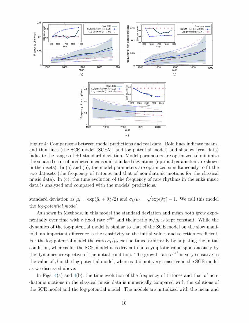
Figure 4: Comparisons between model predictions and real data. Bold lines indicate means,and thin lines (the SCE model (SCEM) and log-potential model) and shadow (real data)indicate the ranges of ±1 standard deviation. Model parameters are optimized to minimizethe squared error of predicted means and standard deviations (optimal parameters are shownin the insets). In (a) and (b), the model parameters are optimized simultaneously to fit thetwo datasets (the frequency of tritones and that of non-diatonic motions for the classicalmusic data). In (c), the time evolution of the frequency of rare rhythms in the enka musicdata is analyzed and compared with the models’ predictions.

standard deviation as µt = exp(µt + σ2t /2) and σt/µt =

√exp(σ2

t )− 1. We call this model

the log-potential model.

As shown in Methods, in this model the standard deviation and mean both grow expo-

nentially over time with a fixed rate eβσ2

and their ratio σt/µt is kept constant. While the

dynamics of the log-potential model is similar to that of the SCE model on the slow mani-

fold, an important difference is the sensitivity to the initial values and selection coefficient.

For the log-potential model the ratio σt/µt can be tuned arbitrarily by adjusting the initial

condition, whereas for the SCE model it is driven to an asymptotic value spontaneously by

the dynamics irrespective of the initial condition. The growth rate eβσ2

is very sensitive to

the value of β in the log-potential model, whereas it is not very sensitive in the SCE model

as we discussed above.

In Figs. 4(a) and 4(b), the time evolution of the frequency of tritones and that of non-

diatonic motions in the classical music data is numerically compared with the solutions of

the SCE model and the log-potential model. The models are initialized with the mean and

10

standard deviation at the earliest time and the model parameters (βT and βN for the SCE

model, and β for the log-potential model) are optimized to minimize the squared error of the

means and standard deviations throughout the time period of the data. If the evolutions

of these two features share the same mechanism, it is reasonable to use the same model

parameters to fit both sets of data. The parameters are thus optimized to fit both sets of

data simultaneously and the optimized values are given inside each figure.

We see that the SCE model can roughly fit both sets of data whereas the log-potential

model can fit only one set of data. Quantitatively, the root mean squared errors for the

tritone and non-diatonic motion data are 4.5× 10−3 and 1.5× 10−2 for the SCE model, and

7.2× 10−3 and 6.1× 10−3 for the log-potential model, respectively. This result indicates not

only that the two sets of data can be explained/predicted by the mechanism described by the

SCE model in a unified way but also that the prediction is not trivial. On the other hand, we

also see some discrepancies between data and model predictions (e.g. in the values of σ/µ).

Such small discrepancies can be explained in several ways: removing the simplifications

assumed for the SCE model may bring small changes in model predictions, as discussed

later, and they may be simply due to statistical/systematic error in the data. If we try to

fit the two sets of data individually using different parameter values, the fitting error for

the log-potential model is slightly smaller than that for the SCE model (see Supplemental

Material).

To examine the ability of the model with different data, Fig. 4(c) illustrates results

of another analysis on a different musical feature extracted from a different dataset. The

dataset is a collection of enka music (a genre of Japanese popular music) compiled and

published by a music publisher [30,31]. Here we focus on the rhythms and use as a feature

the frequency of “rare rhythms” that are defined as bigrams of note values whose ratio

is not one of {1, 1/2, 2, 2/3, 3/2, 1/3, 3, 1/4, 4, 1/6, 6} (see Methods for details). Both the

mean and standard deviation decrease over time, which is qualitatively different from the

previous two cases. For this case, only the SCE model can reproduce the history of the mean

and standard deviation. Predictions for the near future are also provided in Fig. 4(c). As

expected from the decrease of the standard deviation, typicality plays a more influential role

for data selection and the model makes a testable prediction that the mean will converge

in the future. One interpretation of this result is that enka music is considered as a kind of

“soul music” [32] and the evaluators (listeners) would prefer a typical enka song over a novel

one. On the other hand, the log-potential model predicts a linear-like decrease of the mean,

which can be discriminated from the prediction of the SCE model in a near future. The

results show the nontrivial ability of the SCE model to explain and predict the nonlinear

evolution of the enka music and demonstrate that the model is relevant not only for Western

classical music but also for music developed in a different cultural background.

11

Discussion

In conclusion, we have analyzed Western classical music data and found several statistical

evolutionary laws, in particular, steady increase of the mean and standard deviation of

frequencies of rare events and nearly constancy of their ratio, which indicate some driving

force for the evolution of the music style. As a theoretical explanation of the phenomenon,

we have formulated and analyzed SCE models in which creators and evaluators coevolve

by influencing each other through a social selection process. The evaluation function for

the social selection is constructed with the novelty and typicality terms representing cost

required for obtaining and memorizing data in the process of information gathering. We

have shown that when the creator’s and evaluator’s models are beta distributed as observed

in real data and the novelty term is active, the system generally has a slow manifold in

which both the mean and standard deviation grow almost exponentially while their ratio

stays almost constant. This property and the fact that the system’s dynamics are relatively

insensitive to the selection coefficients make the present model more predictive and distinct

from a Darwinian evolutionary model with a logarithmic potential.

It has been demonstrated that the present model can predict the evolution of the Western

classical music data better than a scale-invariant evolutionary model (log-potential model).

The present model had the ability to fit the two kinds of data (frequency of tritones and that

of non-diatonic motions) in a unified way, whereas the log-potential model could only fit

the data individually. From the perspective of the present model, the observed evolution of

the mean and standard deviation of frequencies of musical features that were once rare is a

consequence of pursuing novelty. For the dataset of enka music, both the mean and standard

deviation of the frequency of rare rhythms were found to be decreasing, which indicated that

typicality has more importance than novelty in the selection process. Predictions for the

evolution of this feature that are testable in the next few decades have been made.

In the evolutionary process studied here, the balance between novelty and typicality (i.e.

content dissimilarity and style conformity with respect to past data) plays an essential role.

As we saw in the classical music data and enka music data, relative values of βN and βT

can influence the direction and speed of evolution. We also found that the ratio σ/µ of the

standard deviation and mean is an important metric of evolutionary dynamics, which can

be used to infer from data the relative importance of novelty and typicality in the process

of social selection/evaluation. Once these parameters are determined, the SCE model can

be used to predict the evolution of musical features. Such predictive ability opens the

possibility of new technologies such as hit song prediction [33] and automatic composition

systems that go beyond the ability of simply imitating the style of fixed training data [19,20]

and generate next-generation music.

Since the novelty and typicality biases represent the effective amount of cost necessary

for the evaluator to gather information and are not dependent on particular features of

12

music, they can be important for other types of culture, and the present model can be

useful for analyzing not only music data but also other cultural data. Evolutionary dy-

namics of language [34], other genres of music [6], scientific topics [35], and sociological

phenomena [36, 37] are among topics currently under investigation. Another relevant topic

is the evolution of bird songs, where selection-based learning is considered important [38].

Evolutionary dynamics of bird songs have been studied based on dynamical systems that

describe interaction between generators (singing birds) and imitators [39], which is similar

to the novelty-typicality bias in this study.

Several remarks are made before closing the paper. First, there are multiple possible

ways of extending and relaxing the condition of the minimal model analyzed in this study.

Relaxing the assumption that both the creator and evaluator learn from the same data can

lead to time displacement of their models. For example, if the evaluator learns its model ψt+1

directly from the data Xt, instead of being biased by the evaluation function, then ψt+1 = φt

holds. We can also introduce overlaps between generations or dependence on data created by

more than one past generation. These extensions can change the consequences of the model

quantitatively and can possibly explain the small discrepancies between model prediction

and data in Fig. 4. Systems with multiple creators and evaluators would also be important

for investigating the diversification and specification of cultural styles.

Second, a way to test the present model is to observe the exponential growth of a relevant

feature. However, this is not easy for music data because of the size of each data chunk

(musical piece) is relatively small. A musical piece typically consists of 102 to 103 notes

and thus observing the evolution of a frequency of musical events across some orders of

magnitude is difficult due to data sparseness. It would be possible to alleviate the problem

by extending creator’s and evaluator’s models in a Bayesian manner. Another direction for

experimentally testing the model is to directly examine the evaluation function by means

of music data with social rankings, by an evolutionary experiment involving humans as

evaluators [40], or by psychological experiments [41]. It would also be possible to infer the

form of the evaluation function from such data by machine-learning techniques.

Third, one might think that music styles are transmitted via a set of rules (often called

music theories) and the SCE model does not accord with the reality. It has been argued

that traditional composition rules are not sufficient to describe the actual composition pro-

cess from a computational viewpoint [19], and in fact traditional music theories tell little

about the quantitative nature of music styles [42, 43]. In addition, recent studies on music

informatics have suggested that traditional composition rules can be acquired from data via

statistical learning [21, 44]. Based on these observations, our view is that although those

composition rules may influence the transmission of music styles, the effect of statistical

learning is essential for understanding the evolution of music styles.

Fourth, there are potential sources of social influence that could affect the evolution

of musical styles other than the novelty and typicality biases studied here. These sources

13

include effect of random copying (neutral drift) in a finite population [27], interdependence

among evaluators’ decision [45], active role of creators [46], indirect biases (e.g. publicity)

independent of the data content [2], and psychological biases related to specific musical

features [33]. Our results do not exclude the relevance of these sources to the studied

phenomena of music evolution. The contribution of this work is to propose another possible

source of cultural evolution that can be particularly important when statistical learning

is involved and to provide theoretical results that help identify its relevance in observed

data. Further research is necessary to study the consequences of the SCE model when

it is extended to incorporate those other sources of mutation and social selection and to

identify their individual roles in evolutionary dynamics. It is also important to seek for a

fundamental model that can explain an evolutionary origin of the novelty and typicality

biases in Eq. (3) and can validate the assumption of the Boltzmann distribution in Eq. (2)

as well as the beta distributions observed in the data.

Methods

Data Analysis

A collection of Western classical musical pieces is used for the data analyses in Figs. 1 and

4. The dataset consists of MIDI files of 9,727 pieces by 76 composers downloaded from a

public web page (http://www.kunstderfuge.com). This dataset is compiled in order to

cover a longer period of time than the datasets used in previous studies [5,11] and to enable

noiseless symbolic music analysis. (The dataset used in [11] consists of audio data and the

Peachnote corpus used in [5] contains symbolic music data that are obtained by scanned

sheet music by using music optical character recognition (OCR) software and thus contain

noise.) The 76 composers are those with the largest number of available pieces and obvious

duplications of two or more files for the same piece are avoided by looking at file names. Files

with less than 100 musical notes are also removed. Each MIDI file is parsed and a sequence

of pitches represented by integers in units of semitones is extracted; pitches are ordered

according to their appearance in the file. To extract information on music styles that are

irrelevant of superficial features such as pitch range and absolute key, the sequence of pitch-

class intervals is obtained. Pitches are converted to pitch classes by applying a modulo

operation of divisor 12. Then pitch-class intervals are obtained by taking the difference

between adjacent pitch classes. Note that these intervals include both melodic intervals

and harmonic intervals, which are not distinguished in our analysis. Finally, zero intervals,

which correspond to successions of the same pitch or octave transitions, are dropped because

they dilute other relevant features. Each musical piece is now represented as a sequence of

pitch-class intervals denoted by x = (x1, . . . , xN). Since zero intervals are excluded, there

are 11 types of unigrams and 121 = 112 types of bigrams for pitch-class intervals.

14

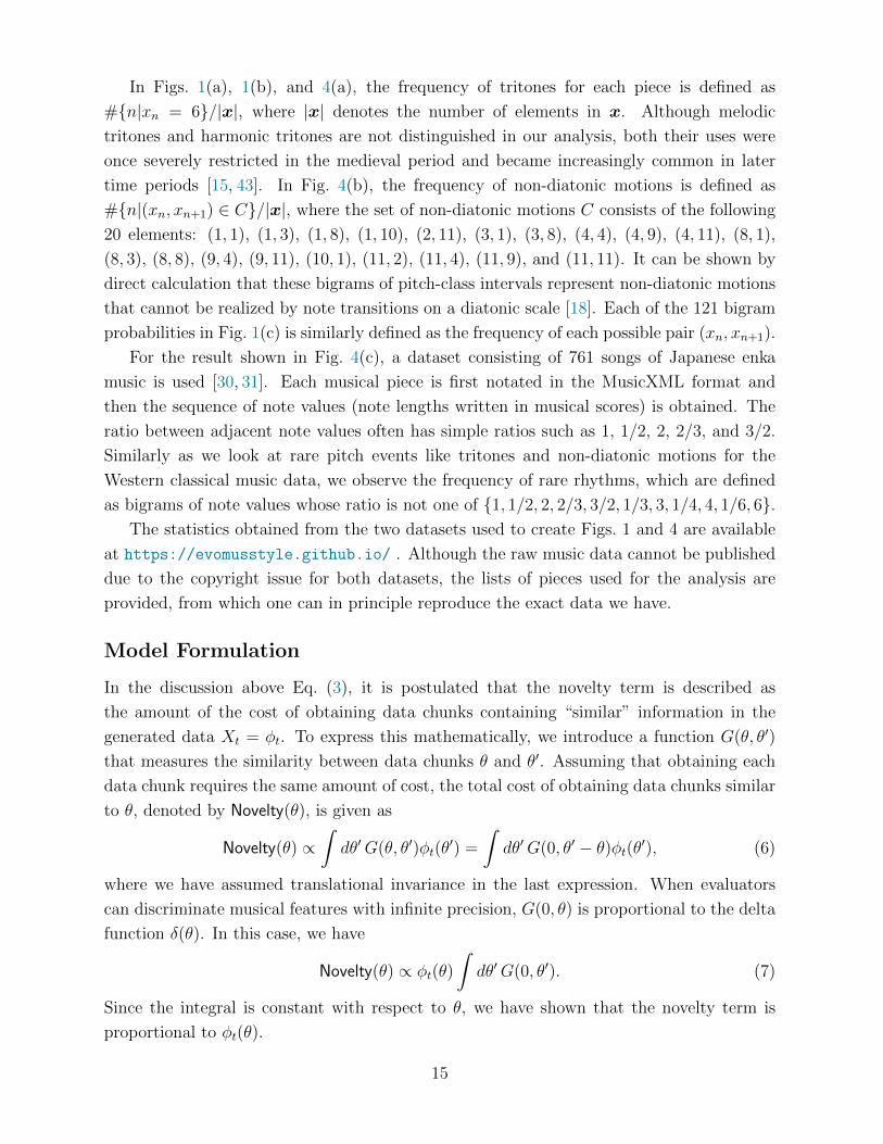
In Figs. 1(a), 1(b), and 4(a), the frequency of tritones for each piece is defined as

#{n|xn = 6}/|x|, where |x| denotes the number of elements in x. Although melodic

tritones and harmonic tritones are not distinguished in our analysis, both their uses were

once severely restricted in the medieval period and became increasingly common in later

time periods [15, 43]. In Fig. 4(b), the frequency of non-diatonic motions is defined as

#{n|(xn, xn+1) ∈ C}/|x|, where the set of non-diatonic motions C consists of the following

20 elements: (1, 1), (1, 3), (1, 8), (1, 10), (2, 11), (3, 1), (3, 8), (4, 4), (4, 9), (4, 11), (8, 1),

(8, 3), (8, 8), (9, 4), (9, 11), (10, 1), (11, 2), (11, 4), (11, 9), and (11, 11). It can be shown by

direct calculation that these bigrams of pitch-class intervals represent non-diatonic motions

that cannot be realized by note transitions on a diatonic scale [18]. Each of the 121 bigram

probabilities in Fig. 1(c) is similarly defined as the frequency of each possible pair (xn, xn+1).

For the result shown in Fig. 4(c), a dataset consisting of 761 songs of Japanese enka

music is used [30, 31]. Each musical piece is first notated in the MusicXML format and

then the sequence of note values (note lengths written in musical scores) is obtained. The

ratio between adjacent note values often has simple ratios such as 1, 1/2, 2, 2/3, and 3/2.

Similarly as we look at rare pitch events like tritones and non-diatonic motions for the

Western classical music data, we observe the frequency of rare rhythms, which are defined

as bigrams of note values whose ratio is not one of {1, 1/2, 2, 2/3, 3/2, 1/3, 3, 1/4, 4, 1/6, 6}.The statistics obtained from the two datasets used to create Figs. 1 and 4 are available

at https://evomusstyle.github.io/ . Although the raw music data cannot be published

due to the copyright issue for both datasets, the lists of pieces used for the analysis are

provided, from which one can in principle reproduce the exact data we have.

Model Formulation

In the discussion above Eq. (3), it is postulated that the novelty term is described as

the amount of the cost of obtaining data chunks containing “similar” information in the

generated data Xt = φt. To express this mathematically, we introduce a function G(θ, θ′)

that measures the similarity between data chunks θ and θ′. Assuming that obtaining each

data chunk requires the same amount of cost, the total cost of obtaining data chunks similar

to θ, denoted by Novelty(θ), is given as

Novelty(θ) ∝∫dθ′G(θ, θ′)φt(θ

′) =

∫dθ′G(0, θ′ − θ)φt(θ′), (6)

where we have assumed translational invariance in the last expression. When evaluators

can discriminate musical features with infinite precision, G(0, θ) is proportional to the delta

function δ(θ). In this case, we have

Novelty(θ) ∝ φt(θ)

∫dθ′G(0, θ′). (7)

Since the integral is constant with respect to θ, we have shown that the novelty term is

proportional to φt(θ).

15

Model Analysis

The parameters at and bt of the beta distribution are in one-to-one correspondence with the

mean µt and standard deviation σt as follows.

µt =at

at + bt(8)

σt =1

at + bt

√atbt

at + bt + 1(9)

σt/µt =√

(1− µt)/(at + µt) (10)

We focus on the case 1 < at < bt, which leads to µt < 1/2 and σt < µt, and in particular the

regime where µt is small, as in the main text. When µt � 1, Eq. (8) indicates that at � bt,

and then µt ' at/bt, σt '√at/bt, and σt/µt ' 1/

√at.

The behaviour of the SCE model defined in Eqs. (1) and (4) for the case βT > 0 and

βN = 0 can be understood from the following analysis. Eq. (4) yields the following equations.

at+1 − 1 = (1 + βT )(at − 1) (11)

bt+1 − 1 = (1 + βT )(bt − 1) (12)

The fact that σt+1 < σt, which is intuitively trivial, can be formally checked by differentiating

the following quantity with respect to βT :

h(βT ) = σ2t+1 =

[at + βT (at − 1)][bt + βT (bt − 1)]

[at + bt + βT (at + bt − 2)]2[at + bt + βT (at + bt − 2) + 1], (13)

where we have used Eq. (9). We can then show ∂h/∂βT < 0 for βT > 0. By noting

that the transformation in Eqs. (11) and (12) for any finite βT can be realized by iterating

infinitesimal transformations, it has been shown that σt+1 < σt. By recursively applying

Eqs. (11) and (12) and substituting the result into Eq. (9), we can also see that

σt ∼1

(1 + βT )t/2(a0 − 1)(b0 − 1)

(a0 + b0 − 2)3→ 0 (t→∞). (14)

We can show µt+1 < µt directly in a similar manner. Alternatively, one can understand

this by looking at the mode (peak position)

kt =at − 1

at + bt − 2. (15)

We can easily show that kt < µt and kt+1 = kt, which means that the peak position

is invariant under the dynamics. Since the difference µt − kt decreases as the standard

16

deviation σt decreases, the result σt+1 < σt indicates µt+1 < µt. The mean µt will converge

to the mode kt since σt → 0 as t→∞.

For the case of βN > 0 and βT = 0, we gave an intuitive argument in the main text that

a slow manifold is formed where σ/µ is almost constant and slightly less than unity. As

discussed there, this slow manifold is formed because σ/µ is decreased by an update when it

is close to unity, which is in turn due to the boundary at zero and the resulting asymmetric

shape of the beta distribution. Here we provide some mathematical analyses to support

this intuitive argument. First, we show that the heights of the two peaks of φt = φte−βNφt

are equal. The position of the right and left peaks (denoted by θ+ and θ−) are obtained by

solving the following equation:

0 =∂φt(θ)

∂θ=∂φt(θ)

∂θe−βNφt(θ)(1− βNφt(θ)). (16)

This yields φt(θ±) = 1/βN . Substituting this back into φt, we have φt(θ±) = 1/(eβN), which

is the height of the peaks. Thus the contributions of the two peaks for the determination

of φt+1 are characterized by their position (mean) and width. As can be seen in Fig. 3(e),

when σ/µ is close to unity the width of the left peak is so much less than that of the right

peak because of the boundary at zero that the φt+1 is determined dominantly by the right

peak.

Next, for the regime of parameters of our interest (µt � 1), σt/µt ' 1/√at holds.

This means that the ratio σt/µt is smaller if at is larger. That is, the gradient of the beta

distribution near zero is smaller. As we see in Fig. 3(e), when the next-generation creator’s

model φt+1 is dominantly determined by the right peak of φt, at+1 > at generally holds. This

shows that σt+1/µt+1 < σt/µt when σt/µt is close to unity. Moreover, one finds from the

relation φt(θ±) = 1/(eβN) that θ+ increase as βN becomes larger, which in turn indicates

that at becomes larger. Thus, for larger βN , the asymptotic value of σt/µt tends to be

smaller.

For the case both βN , βT > 0, a slow manifold is formed in the regime where µt and σt

are small. To understand this, first note that at � bt, µt ' at/bt, and σt '√at/bt hold

for µt � 1. The effect of the typicality term can be written as at+1 = at + βT (at − 1) and

bt+1 ' (1 + βT )bt from Eqs. (11) and (12), which indicates the following.

σtµt� 1 ⇒ µt+1 ' µt, σt+1 '

1√1 + βT

σt. (17)

σtµt' 1 ⇒ µt+1 '

1

1 + βTµt, σt+1 '

1

1 + βTσt. (18)

This means that if σt/µt � 1 the typicality term decreases this ratio by a constant factor

of 1/√

1 + βT . On the other hand, the novelty term increases it by a factor that becomes

larger for smaller σt (one can confirm this for example in Fig. 3(b)). Thus, the effect of the

17

novelty term dominates over that of the typicality term for sufficiently small σt, in which

case σt/µt increases. When σt/µt ' 1, the effect of the typicality term is negligible, so

the slow manifold is formed due to the effect of the novelty term. On the slow manifold,

the typicality term acts on the mean µt as in Eq. (18), which has the effect of a constant

reduction factor, and the novelty term acts as illustrated in Fig. 3(g), which has a larger

effect for smaller µt. Thus, for sufficiently small µt, the dynamics is dominated by the

novelty term, leading to a nearly exponential growth on the slow manifold.

The dynamics of the log-potential model can be solved as follows. Substituting Eq. (5)

and Rt = ln θ into Eq. (2), we have

φt(θ) =1√

2πσtθexp

[− 1

2σ2t

{ln θ − (µt + βσ2

t )}2

+ const

]. (19)

By solving for the parameters of φt+1 with the same mean and standard deviation, we find

that

σt+1 = σt =: σ, (20)

µt+1 = µt + βσ2. (21)

Using the relations between (µt, σt) and (µt, σt) given in the main text, we obtain

σt+1/µt+1 = σt/µt, (22)

µt+1 = µteβσ2

, (23)

as claimed in the main text.

Additional Information

The authors declare no competing interests.

Acknowledgment

The authors would like to thank Masahiko Ueda and Nobuto Takeuchi for useful discussions

and Kazuyoshi Yoshii for sharing the enka music data. This work was in part supported by

Grant-in-Aid for Scientific Research on Innovative Areas No. 17H06386 from the Ministry

of Education, Culture, Sports, Science and Technology (MEXT) of Japan and Grants-in-

Aid for Scientific Research Nos. 16J05486, 16H02917, 16K00501, and 19K20340 from Japan

Society for the Promotion of Science (JSPS). The work of E.N. was supported by the JSPS

Postdoctoral Research Fellowship.

18

Data Availability Statement

The datasets generated and analyzed during the current study are available in the GitHub

repository, https://evomusstyle.github.io/. See also Data Analysis section above.

References

[1] J. M. Smith and E. Szathmary, The Major Transitions in Evolution, Oxford University

Press, 1997.

[2] R. Boyd and P. J. Richerson, Culture and the Evolutionary Process, The University of

Chicago Press, 1985.

[3] L. L. Cavalli-Sforza and M. W. Feldman, Cultural Transmission and Evolution, Prince-

ton University Press, 1981.

[4] J. Serra, A. Corral, M. Boguna, M. Haro, and J. L. Arcos, “Measuring the Evolution

of Contemporary Western Popular Music,” Scientific Reports, 2(521), pp. 1–6, 2012.

[5] P. H. R. Zivic, F. Shifres, and G. A. Cecchi, “Perceptual Basis of Evolving Western

Musical Styles,” Proc. Natl. Acad. Sci., 110(24), pp. 10034–10038, 2013.

[6] M. Mauch, R. M. MacCallum, M. Levy, and A. M. Leroi, “The Evolution of Popular

Music: USA 1960–2010,” R. Soc. Open Sci., 2(150081), pp. 1–10, 2015.

[7] H. Honing, C. ten Cate, I. Peretz, and S. E. Trehub, “Without It No Music: Cognition,

Biology and Evolution of Musicality,” Phil. Trans. R. Soc. B, 370(20140088), pp. 1–8,

2015.

[8] A. Ravignani, T. Delgado, and S. Kirby, “Musical Evolution In the Lab Exhibits Rhyth-

mic Universals,” Nature Human Behaviour, 1(0007), pp. 1–7, 2016.

[9] S. Le Bomin, G. Lecointre, and E. Heyer, “The Evolution of Musical Diversity: The

Key Role of Vertical Transmission,” Plos One, 11(3)(e0151570), pp. 1–17, 2016.

[10] P. E. Savage, “Cultural Evolution of Music,” Palgrave Communications, 5(16), pp. 1–

12, 2019.

[11] C. Weiß, M. Mauch, S. Dixon, and M. Muller, “Investigating Style Evolution of Western

Classical Music: A Computational Approach,” Musicae Scientiae, 23(4), pp. 486–507,

2019, DOI: 10.1177/1029864918757595.

[12] R. O. Morris, Foundations of Practical Harmony and Counterpoint (2nd ed.), Macmil-

lan, 1931.

[13] M. Lassig, V. Mustonen, and A. M. Walczak, “Predicting Evolution,” Nature Ecology

& Evolution, 1(3), pp. 0077, 2017.

[14] S. Kostka, D. Payne, and B. Almen, Tonal Harmony with an Introduction to Twentieth-

Century Music (7th ed.), McGraw-Hill, 2013.

19

[15] J. P. Burkholder, D. J. Grout, and C. V. Palisca, A History of Western Music (8th

ed.), W. W. Norton & Company, 2010.

[16] C. L. Krumhansl, Cognitive Foundations of Musical Pitch, Oxford Univ. Press, 1990.

[17] J. H. McDermott, A. F. Schultz, E. A. Undurraga, and R. A. Godoy, “Indifference to

Dissonance in Native Amazonians Reveals Cultural Variation in Music Perception,”

Nature, 535, pp. 547–550, 2016.

[18] E. Nakamura and S. Takaki, “Characteristics of Polyphonic Music Style and Markov

Model of Pitch-Class Intervals,” in Proc. 5th Mathematics and Computation in Music,

pp. 109–114, 2015.

[19] K. Ebcioglu, “An Expert System for Harmonizing Chorales in the Style of J. S. Bach,”

Journal of Logic Programming, 8(1), pp. 145–185, 1990.

[20] F. Pachet and P. Roy, “Markov Constraints: Steerable Generation of Markov Se-

quences,” Constraints, 16(2), pp. 148–172, 2011.

[21] H. Tsushima, E. Nakamura, K. Itoyama, and K. Yoshii, “Generative Statistical Models

with Self-Emergent Grammar of Chord Sequences,” J. New Music Res., 47(3), pp. 226–

248, 2018.

[22] M. Ettlinger, E. H. Margulis, and P. Wong, “Implicit Memory in Music and Language,”

Frontiers in Psychology, 2(211), pp. 1–10, 2011.

[23] J. Hofbauer and K. Sigmund, Evolutionary Games and Population Dynamics, Cam-

bridge University Press, 1998.

[24] T. Hashimoto and T. Ikegami, “Emergence of Net-Grammar in Communicating

Agents,” BioSystems, 38, pp. 1–14, 1996.

[25] S. Kirby, “Spontaneous Evolution of Linguistic Structure – An Iterated Learning Model

of the Emergence of Regularity and Irregularity,” IEEE Trans. Evol. Comp., 5(2),

pp. 102–110, 2001.

[26] M. A. Nowak, N. L. Komarova, and P. Niyogi, “Evolution of Universal Grammar,”

Science, 291, pp. 114–118, 2001.

[27] R. A. Bentley, C. P. Lipo, H. A. Herzog, and M. W. Hahn, “Regular Rates of Popular

Culture Change Reflect Random Copying,” Evolution and Human Behavior, 48(3),

pp. 151–158, 2007.

[28] E. Newman ed., Memoirs of Hector Berlioz, Alfred A. Knopf, 1932.

[29] T. M. Cover and J. A. Thomas, Elements of Information Theory (2nd ed), John Wiley

& Sons, 2006.

[30] Y. Goto (ed.), Grand Collection of Enka Songs by Male Singers 5th Ed. (in Japanese),

Zen-on Music Co., 2016.

[31] Y. Goto (ed.), Grand Collection of Enka Songs by Female Singers 5th Ed. (in Japanese),

Zen-on Music Co., 2016.

20

[32] Y. Wajima (transl. by K. D. Hopkins), Creating Enka, The “Soul of Japan” in the

Postwar Era, Public Bath Press, 2018.

[33] D. Herremans, D. Martens, and K. Sorensen, “Dance Hit Song Prediction,” J. New

Music Res., 43(3), pp. 291–302, 2014.

[34] J.-B. Michel, Y. K. Shen, A. P. Aiden, A. Veres, M. K. Gray, The Google Books Team,

J. P. Pickett, D. Hoiberg, D. Clancy, P. Norvig, J. Orwant, S. Pinker, M. A. Nowak,

and E. L. Aiden, “Quantitative Analysis of Culture Using Millions Of Digitized Books,”

Science, 331(6014), pp. 176–182, 2011.

[35] T. L. Griffiths and M. Steyvers, “Finding Scientific Topics,” Proc. Natl. Acad. Sci.,

101(suppl 1), pp. 5228–5235, 2004.

[36] C. Castellano, M. Marsili, and A. Vespignani, “Nonequilibrium Phase Transition in a

Model for Social Influence,” Phys. Rev. Lett., 85(16), pp. 3536–3539, 2000.

[37] D. M. Abrams, H. A. Yaple, and R. J. Wiener, “Dynamics of Social Group Competition:

Modeling the Decline of Religious Affiliation,” Phys. Rev. Lett., 107(088701), pp. 1–4,

2011.

[38] D. A. Nelson and P. Marler, “Selection-Based Learning in Bird Song Development,”

Proc. Natl. Acad. Sci., 91(22), pp. 10498–10501, 1994.

[39] J. Suzuki and K. Kaneko, “Imitation Games,” Physica D, 75, pp. 328–342, 1994.

[40] R. M. MacCallum, M. Mauch, A. Burt, and A. M. Leroi, “Evolution of Music by Public

Choice,” Proc. Natl. Acad. Sci., 109(30), pp. 12081–12086, 2012.

[41] D. Huron, Sweet Anticipation: Music and the Psychology of Expectation, The MIT

Press, 2006.

[42] R. L. Crocker, A History of Musical Style, McGraw-Hill, 1966.

[43] D. de la Motte, Harmonielehre, Barenreiter-Verlag, 1976.

[44] M. Allan and C. K. I. Williams, “Harmonising Chorales by Probabilistic Inference,” in

Proc. 17th Advances in Neural Information Processing Systems, pp. 25–32, 2004.

[45] M. J. Salganik, P. S. Dodds, and D. J. Watts, “Experimental Study of Inequality and

Unpredictability in an Artificial Cultural Market,” Science, 311(5762), pp. 854–856,

2006.

[46] N. Claidiere, S. Kirby, and D. Sperber, “Effect of Psychological Bias Separates Cultural

from Biological Evolution,” Proc. Natl. Acad. Sci., 109(51), pp. E3526, 2012.

Author Contribution

Both authors designed the work and wrote the main manuscript text. EN conducted nu-

merial experiments and prepared all the figures. Both authors reviewed the manuscript.

21

Supplemental Material for

“Statistical Evolutionary Laws in Music Styles”

Eita Nakamura1∗ and Kunihiko Kaneko2†

1 The Hakubi Center for Advanced Research and Graduate School of Informatics,

Kyoto University, Sakyo, Kyoto 606-8501, Japan2 Department of Basic Science, University of Tokyo, Meguro, Tokyo 153-8902, Japan

Contents

1 Analysis on the Classical Music Data 22

2 Analysis of the SCE models for other distributions 23

3 Additional Comparison between the SCE Model and the Log-Potential

Model 25

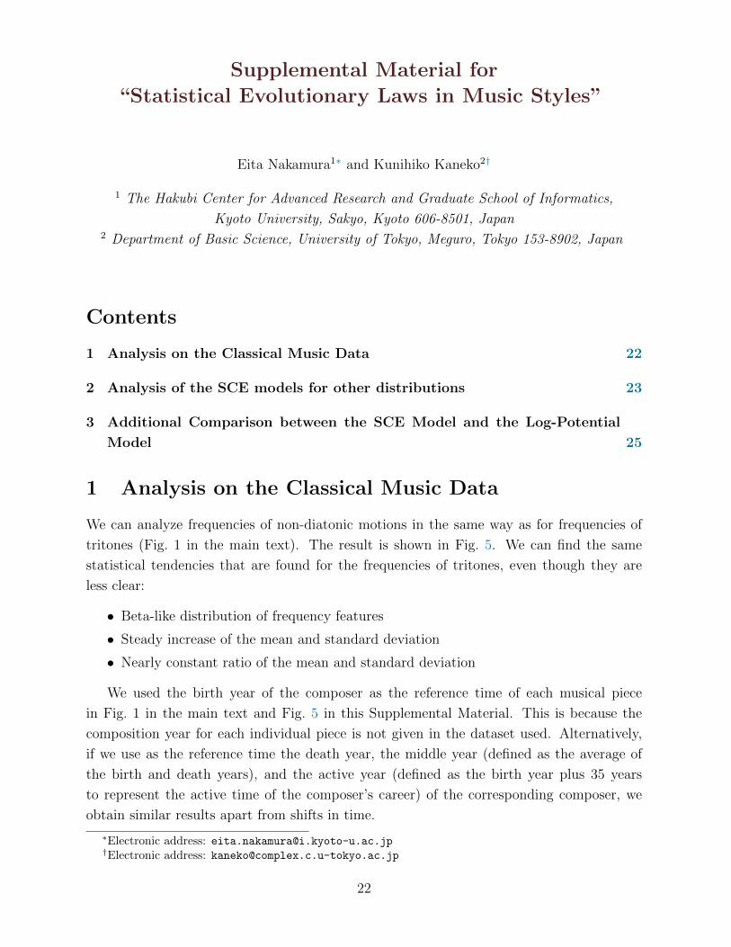
1 Analysis on the Classical Music Data

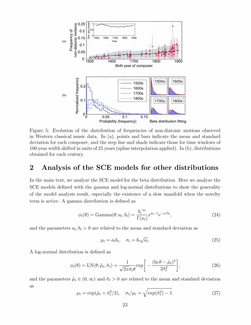
We can analyze frequencies of non-diatonic motions in the same way as for frequencies of

tritones (Fig. 1 in the main text). The result is shown in Fig. 5. We can find the same

statistical tendencies that are found for the frequencies of tritones, even though they are

less clear:

• Beta-like distribution of frequency features

• Steady increase of the mean and standard deviation

• Nearly constant ratio of the mean and standard deviation

We used the birth year of the composer as the reference time of each musical piece

in Fig. 1 in the main text and Fig. 5 in this Supplemental Material. This is because the

composition year for each individual piece is not given in the dataset used. Alternatively,

if we use as the reference time the death year, the middle year (defined as the average of

the birth and death years), and the active year (defined as the birth year plus 35 years

to represent the active time of the composer’s career) of the corresponding composer, we

obtain similar results apart from shifts in time.

∗Electronic address: eita.nakamura@i.kyoto-u.ac.jp†Electronic address: kaneko@complex.c.u-tokyo.ac.jp

22

(a)

(b)

Fre

quen

cy o

fno

n-di

aton

ic m

otio

ns

Birth year of composer

0

0.1

0.2

0 0.05 0.1 0.15

Nor

mal

ized

freq

uenc

y

Probability (frequency)

1500s1600s1700s1800s

1500s 1600s

1700s 1800s

Beta distribution fitting

0

0.05

0.1

0.15

0.2

0.25

1500 1600 1700 1800 1900

0

0.5

1

1500 1600 1700 1800 1900(Std

. dev

.)/m

ean

Year

Figure 5: Evolution of the distribution of frequencies of non-diatonic motions observedin Western classical music data. In (a), points and bars indicate the mean and standarddeviation for each composer, and the step line and shade indicate those for time windows of100-year width shifted in units of 25 years (spline interpolation applied). In (b), distributionsobtained for each century.

2 Analysis of the SCE models for other distributions

In the main text, we analyze the SCE model for the beta distribution. Here we analyze the

SCE models defined with the gamma and log-normal distributions to show the generality

of the model analysis result, especially the existence of a slow manifold when the novelty

term is active. A gamma distribution is defined as

φt(θ) = Gamma(θ; at, bt) =b−att

Γ(at)xat−1e−x/bt , (24)

and the parameters at, bt > 0 are related to the mean and standard deviation as

µt = atbt, σt = bt√at. (25)

A log-normal distribution is defined as

φt(θ) = LN(θ; µt, σt) =1√

2πσtθexp

[− (ln θ − µt)2

2σ2t

], (26)

and the parameters µt ∈ (0,∞) and σt > 0 are related to the mean and standard deviation

as

µt = exp(µt + σ2t /2), σt/µt =

√exp(σ2

t )− 1. (27)

23

0

0.05

0.1

0.15

1500 1600 1700 1800 1900

Fre

quen

cy o

f trit

ones

Birth year of composer

birth yearmiddle yearactive yeardeath year

0

0.5

1

1500 1600 1700 1800 1900(Std

. dev

.)/m

ean

Year

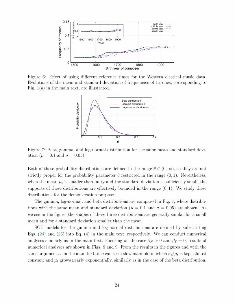
Figure 6: Effect of using different reference times for the Western classical music data.Evolutions of the mean and standard deviation of frequencies of tritones, corresponding toFig. 1(a) in the main text, are illustrated.

0 0.1 0.2 0.3 0.4

Pro

babi

lity

dist

ribut

ion

Beta distributionGamma distributionLog-normal distribution

θ

Figure 7: Beta, gamma, and log-normal distribution for the same mean and standard devi-ation (µ = 0.1 and σ = 0.05).

Both of these probability distributions are defined in the range θ ∈ (0,∞), so they are not

strictly proper for the probability parameter θ restricted in the range (0, 1). Nevertheless,

when the mean µt is smaller than unity and the standard deviation is sufficiently small, the

supports of these distributions are effectively bounded in the range (0, 1). We study these

distributions for the demonstration purpose.

The gamma, log-normal, and beta distributions are compared in Fig. 7, where distribu-

tions with the same mean and standard deviation (µ = 0.1 and σ = 0.05) are shown. As

we see in the figure, the shapes of these three distributions are generally similar for a small

mean and for a standard deviation smaller than the mean.

SCE models for the gamma and log-normal distributions are defined by substituting

Eqs. (24) and (26) into Eq. (4) in the main text, respectively. We can conduct numerical

analyses similarly as in the main text. Focusing on the case βN > 0 and βT = 0, results of

numerical analyses are shown in Figs. 8 and 9. From the results in the figures and with the

same argument as in the main text, one can see a slow manifold in which σt/µt is kept almost

constant and µt grows nearly exponentially, similarly as in the case of the beta distribution.

24

βT = 0, βN = 0.3(a)

Growth

ofmeanµt+

1/µt

Mean µt

σt+

1/µt+

1

(b)

(c)

Mean µt

110−110−2

St.dev.σt

1

10−1

10−2

10−3

σt = µt

1

10

10-4 10-3 10-2 10-1

βN = 3

βN = 0.1

0.01

0.1

1

0.01

0.1

1

0.1 1

βN = 3

βN = 0.1

µt = 10−1

µt = 10−2

µt = 10−3

µt = 10−4

σt/µt

Figure 8: Numerical analysis of the SCE model defined with the gamma distribution for thecase βN > 0 and βT = 0. (a) Orbits of the SCE model (b) Dynamics of the ratio σt/µt. (c)Growth of the mean around the slow manifold (σt/µt = 0.4).

3 Additional Comparison between the SCE Model and

the Log-Potential Model

In Figs. 4(a) and 4(b) of the main text, we compared how the SCE model and the log-

potential model can fit the real data of classical music. There, the model parameters were

optimized to best fit the two sets of data (frequencies of tritones and non-diatonic motions).

Here we report the results when the model parameters are fitted to the two sets of data

individually.

The results are shown in Figs. 10(a) and 10(b). The root mean squared errors of the

(tritone, non-diatonic motion) data are (4.4 × 10−3, 7.2 × 10−3) for the SCE model and

(3.0 × 10−3, 5.8 × 10−3) for the log-potential model. Compared to the results in the main

text, these results show that for the SCE model the precision of the individual fit is similar

to that of the simultaneous fit, and that the log-potential model can fit individual data

slightly better than the SCE model. This shows that although the log-potential model is

flexible for fitting individual sets of data, it cannot fit both sets of data simultaneously,

confirming that it is not trivial to fit both sets of data in a unified manner.

25

βT = 0, βN = 0.3(a)

Growth

ofmeanµt+

1/µ

t

Mean µt

σt+

1/µt+

1

(b)

(c)

Mean µt

110−110−2

St.dev.σt

1

10−1

10−2

10−3

σt/µt

σt = µt

1

10

10-4 10-3 10-2 10-1

βN = 3

βN = 0.1

0.01

0.1

1

0.01

0.1

1

0.1 1

βN = 3

βN = 0.1

µt = 10−1

µt = 10−2

µt = 10−3

µt = 10−4

Figure 9: Numerical analysis of the SCE model defined with the log-normal distribution forthe case βN > 0 and βT = 0. (a) Orbits of the SCE model (b) Dynamics of the ratio σt/µt.(c) Growth of the mean around the slow manifold (σt/µt = 0.4).

(a) (b)

Real data

Log potential ( : 1.11)SCEM ( : 0.12, : 0.07)

ββT βN

0

0.05

0.1

0.15

1500 1600 1700 1800 1900

Fre

quen

cy o

f trit

ones

Year

0.4

0.6

1500 1600 1700 1800 1900

(Std

. dev

.)/m

ean

Year

0

0.05

0.1

0.15

1500 1600 1700 1800 1900

Fre

quen

cy o

f non

-dia

toni

c m

otio

ns

Year

0.4

0.6

0.8

1

1500 1600 1700 1800 1900

(Std

. dev

.)/m

ean

Year

Real data

Log potential ( : 0.39)SCEM ( : 0, : 0.05)

ββT βN

Figure 10: Comparisons between model predictions and real data. Bold lines indicate means,and thin lines and shadow indicate the ranges of ±1 standard deviation. Model parametersare optimized individually to fit the two datasets to minimize the squared error of predictedmeans and standard deviations (optimal parameters are shown in the insets).

26