
Statistical distributions of singular vectors for tropical cyclones affecting Korea over a 10-year...
16
ORIGINAL PAPER Statistical distributions of singular vectors for tropical cyclones affecting Korea over a 10-year period Sei-Young Park • Hyun Mee Kim • Tae-Young Lee • Michael C. Morgan Received: 16 July 2012 / Accepted: 7 March 2013 / Published online: 28 March 2013 Ó The Author(s) 2013. This article is published with open access at Springerlink.com Abstract To investigate the statistical sensitivity distri- butions of tropical cyclone (TC) forecasts over the Korean Peninsula, total energy (TE) singular vectors (SVs) were calculated and evaluated over a 10-year period. TESVs were calculated using the fifth-generation Pennsylvania State University/National Center for Atmospheric Research Mesoscale Model (MM5) and its tangent linear and adjoint models with a Lanczos algorithm over a 48-h period. Chosen cases were 21 TCs that affected the Korean Pen- insula among 230 TCs that were generated in the western North Pacific from 2001 to 2010. Sensitive regions indi- cated by TESVs were mainly located near mid-latitude troughs and TC centers but varied depending on TC track and environmental conditions such as subtropical high and mid-latitude trough. The cases were classified into three groups by clustering TC tracks based on the finite mixture model. The two groups that passed through the western and southern sea of the Korean Peninsula had maximally sen- sitive regions in the mid-latitude trough and largely sen- sitive regions around the TC center, while the other group that passed straight through the eastern sea of the Korean Peninsula had maximally sensitive regions near the north- eastern region of the TC center. Vertically, the former two clustered groups had the westerly tilted TESVs and potential vorticity structures under the mid-latitude troughs at the initial time, indicating the TCs were in a baroclinic environment. Conversely, the straight-moving TCs were not in a baroclinic environment. Based on the results in the present study, the TCs moving toward a fixed verification region over the Korean Peninsula have different sensitivity regions and structures according to their moving tracks and characteristic environmental conditions, which may pro- vide guidance for targeted observations of TCs affecting the Korean Peninsula. 1 Introduction Considerable effort has been made to increase the accuracy of tropical cyclone (TC) forecasts by studying TC dynamics and structures (Kurihara and Tuleya 1974; Frank 1977a, b; Wang 2002; Kwon and Frank 2005, 2008) and by investigating the relationship between TCs and the environment using obser- vational or reanalysis data from numerical weather prediction (NWP) models (Holland and Wang 1995; Ho et al. 2004; Byun and Lee 2012), as well as by developing an NWP model for TCs (Rappaport et al. 2009; Dorst 2007). When considering the accuracy of the NWP model, there are two types of error: the model error and the initial condition uncertainties. Adaptive (or targeted) observations have been applied to TCs to increase the accuracy of TC forecasts by decreasing the initial condition uncertainties (Peng and Reynolds 2005, 2006; Kim and Jung 2006, 2009a, b; Kim et al. 2011a; Jung et al. 2012; Majumdar et al. 2006; Wu et al. 2007, 2009a, b; Lang et al. 2012). The observational regions detected by adaptive observation strategies are called sensitive regions because the obser- vations in those regions may have a large influence on enhancing weather forecasts (Kim et al. 2004a). Singular Responsible editor: M. Kaplan. S.-Y. Park H. M. Kim (&) T.-Y. Lee Department of Atmospheric Sciences, Yonsei University, 50 Yonsei-ro, Seodaemun-gu, Seoul 120-749, Republic of Korea e-mail: [email protected] M. C. Morgan Department of Atmospheric and Oceanic Sciences, University of Wisconsin–Madison, Madison, USA 123 Meteorol Atmos Phys (2013) 120:107–122 DOI 10.1007/s00703-013-0247-7
-
Upload
tae-young-lee -
Category
Documents
-
view
212 -
download
0
Transcript of Statistical distributions of singular vectors for tropical cyclones affecting Korea over a 10-year...
ORIGINAL PAPER
Statistical distributions of singular vectors for tropical cyclonesaffecting Korea over a 10-year period
Sei-Young Park • Hyun Mee Kim • Tae-Young Lee •
Michael C. Morgan
Received: 16 July 2012 / Accepted: 7 March 2013 / Published online: 28 March 2013
� The Author(s) 2013. This article is published with open access at Springerlink.com
Abstract To investigate the statistical sensitivity distri-
butions of tropical cyclone (TC) forecasts over the Korean
Peninsula, total energy (TE) singular vectors (SVs) were
calculated and evaluated over a 10-year period. TESVs
were calculated using the fifth-generation Pennsylvania
State University/National Center for Atmospheric Research
Mesoscale Model (MM5) and its tangent linear and adjoint
models with a Lanczos algorithm over a 48-h period.
Chosen cases were 21 TCs that affected the Korean Pen-
insula among 230 TCs that were generated in the western
North Pacific from 2001 to 2010. Sensitive regions indi-
cated by TESVs were mainly located near mid-latitude
troughs and TC centers but varied depending on TC track
and environmental conditions such as subtropical high and
mid-latitude trough. The cases were classified into three
groups by clustering TC tracks based on the finite mixture
model. The two groups that passed through the western and
southern sea of the Korean Peninsula had maximally sen-
sitive regions in the mid-latitude trough and largely sen-
sitive regions around the TC center, while the other group
that passed straight through the eastern sea of the Korean
Peninsula had maximally sensitive regions near the north-
eastern region of the TC center. Vertically, the former two
clustered groups had the westerly tilted TESVs and
potential vorticity structures under the mid-latitude troughs
at the initial time, indicating the TCs were in a baroclinic
environment. Conversely, the straight-moving TCs were
not in a baroclinic environment. Based on the results in the
present study, the TCs moving toward a fixed verification
region over the Korean Peninsula have different sensitivity
regions and structures according to their moving tracks and
characteristic environmental conditions, which may pro-
vide guidance for targeted observations of TCs affecting
the Korean Peninsula.
1 Introduction
Considerable effort has been made to increase the accuracy of
tropical cyclone (TC) forecasts by studying TC dynamics and
structures (Kurihara and Tuleya 1974; Frank 1977a, b; Wang
2002; Kwon and Frank 2005, 2008) and by investigating the
relationship between TCs and the environment using obser-
vational or reanalysis data from numerical weather prediction
(NWP) models (Holland and Wang 1995; Ho et al. 2004;
Byun and Lee 2012), as well as by developing an NWP model
for TCs (Rappaport et al. 2009; Dorst 2007).
When considering the accuracy of the NWP model,
there are two types of error: the model error and the initial
condition uncertainties. Adaptive (or targeted) observations
have been applied to TCs to increase the accuracy of TC
forecasts by decreasing the initial condition uncertainties
(Peng and Reynolds 2005, 2006; Kim and Jung 2006,
2009a, b; Kim et al. 2011a; Jung et al. 2012; Majumdar
et al. 2006; Wu et al. 2007, 2009a, b; Lang et al. 2012). The
observational regions detected by adaptive observation
strategies are called sensitive regions because the obser-
vations in those regions may have a large influence on
enhancing weather forecasts (Kim et al. 2004a). Singular
Responsible editor: M. Kaplan.
S.-Y. Park � H. M. Kim (&) � T.-Y. Lee
Department of Atmospheric Sciences, Yonsei University,
50 Yonsei-ro, Seodaemun-gu, Seoul 120-749,
Republic of Korea
e-mail: [email protected]
M. C. Morgan
Department of Atmospheric and Oceanic Sciences,
University of Wisconsin–Madison, Madison, USA
123
Meteorol Atmos Phys (2013) 120:107–122
DOI 10.1007/s00703-013-0247-7
vectors (SVs) have been used to detect regions of high
sensitivity to small perturbations for the purpose of making
adaptive observations (Palmer et al. 1998; Buizza and
Montani 1999; Gelaro et al. 1999; Montani et al. 1999;
Peng and Reynolds 2005, 2006; Kim and Jung 2009a, b)
because they are the fastest growing perturbations during a
specified time period (i.e., the optimization interval) for a
given norm and basic state (Kim and Morgan 2002).
There have been two kinds of studies applying SVs for
TC forecasts. One is a case study and the other is a sta-
tistical or composite analysis applied to many cases. As a
case study, Kim and Jung (2009a) evaluated the SV sen-
sitivities near a TC center and at midlatitude and inter-
preted the dynamical interactions between the recurving
TC and the mid-latitude system. In addition, Kim and Jung
(2009b) investigated the effects of moist physics and norm
on SV structures of Typhoon Usagi (0705). As a composite
analysis, Peng and Reynolds (2006) studied 85 TC cases
that were generated in the western North Pacific from July
to October 2003 and divided them into two groups
(straight- and non-straight moving TCs) to determine the
SV characteristics due to TC movements. Reynolds et al.
(2009) chose 84 cases from the 18 TCs generated in 2006
to investigate SV sensitivities and downstream impacts.
Chen et al. (2009) studied the same cases as Reynolds et al.
(2009) except for the extratropical transition (ET) cases
and focused on the dynamic relationship between TC
evolution and the surrounding synoptic-scale features.
Several observational and simulation studies have already
shown that TC evolution and movements are closely asso-
ciated with the surrounding environment (e.g., the subtropical
ridge and extratropical trough). Wang et al. (1993) found that
TC motion in a baroclinic environment can be sensitive to the
diabatic heating and the vertical structures of both the vortex
and its environment. Holland and Wang (1995) indicated that
recurvature can occur through an unbroken subtropical ridge
at the initial time, but that the mid-latitude trough consider-
ably strengthens the potential for recurvature. Holland and
Wang (1995) further suggested that vorticity and environ-
mental changes in the middle and lower levels may be more
significant for general environmental interactions leading to
recurvature than those in the upper troposphere. Wu et al.
(2009b) stated there are several dynamic systems affecting
the TC motion in the western North Pacific, such as the
subtropical high, the mid-latitude trough, the subtropical jet,
and the southwesterly monsoon.
Previous sensitivity studies using SVs and adjoint sen-
sitivities reaffirm the important relationship between TCs
and surrounding environments on TC movements and
evolution. Nevertheless, none of the previous studies
focused on the TCs affecting the Korean Peninsula over an
extended period. In addition, the previous statistical sen-
sitivity analysis for TCs that occurred in the western North
Pacific focused on several TCs that occurred in specific
years, which may not represent long-term sensitivity
characteristics. Therefore, the present study investigated
the statistical TESV distributions of the TC forecasts
affecting the Korean Peninsula during the past 10 years.
The distinct characteristics of the present study that differ
from the previous studies are that only one case is chosen
for each TC, the experimental period is long (10 years,
from 2001 to 2010), and the verification region is fixed to
the Korean Peninsula for all experiments.
Section 2 describes the methodology and experimental
framework, while Sect. 3 describes the results, and Sect. 4
contains a summary and discussion.
2 Methodology and experimental framework
2.1 Singular vector calculation
As described in Kim and Jung (2009b), the calculation of SVs
involves selecting an initial disturbance with the constraint
that it has the unit amplitude and evolves to have maximum
amplitude in a specified norm after some finite optimization
time. In this study, the initial and final norms used were the
dry total energy (TE) defined by Zou et al. (1997) as:
Ed ¼ZZZ
r;y;x
1
2u02 þ v02 þ w02 þ g
Nh
� �2
h02"
þ 1
qcs
� �2
p02
#dx dy dr; ð1Þ
where Ed is dry TE in a non-hydrostatic model; u0, v0 and w0
are the zonal, meridional, and vertical wind perturbations,
respectively; h0is the potential temperature perturbation; p0
is the pressure perturbation; N, h, q, and cs are the Brunt–
Vaisala frequency, potential temperature, density, and
speed of sound at the reference level (500 hPa), respec-
tively; and x, y, and r denote the zonal, meridional, and
vertical coordinates, respectively.
The amplitude of the perturbation state vector (x0) in the
specific norm C was defined as:
x0ðtÞ; Cx0ðtÞh i ¼ Mx0ð0Þ; CMx0ð0Þh i; ð2Þ
where the inner product is denoted by ;h i, M is the tangent
linear model (TLM) of the non-linear model, and C is the
matrix operator appropriate to the specific norm.
In (2), the state vector at the initial time was assumed to
evolve linearly. The constrained optimization problem
seeks to maximize the amplification factor:
k2 ¼ PMx0ð0Þ;CPMx0ð0Þh ix0ð0Þ;Cx0ð0Þh i ð3Þ
108 S.-Y. Park et al.
123
at the optimization time, where P is a local projection
operator that makes the state vector zero outside a given
domain (Buizza 1994). That domain was the verification
region in the present study. A local projection operator was
employed to optimize the final-time perturbation energy in
a 20� 9 20� box, as in Peng and Reynolds (2006),
Reynolds et al. (2009), and Chen et al. (2009), centered
on the final-time TC position (33.530�N, 128.975�E) that
was the median of the 48-h TC forecast centers and
included the Korean Peninsula.
The maximum of the ratio in (3) is realized when x0ð0Þ is
the leading SV of TLM M for the C norm, that is, when
x0ð0Þ satisfies the following:
MT PT CPMx0ð0Þ ¼ k2Cx0ð0Þ: ð4Þ
The generalized eigenvalue problem in (4) can be
reduced to an ordinary eigenvalue problem by multiplying
both sides with the inverse of the square root of C. Then a
Lanczos-type algorithm (e.g., Ehrendorfer and Errico
1995) is used to solve for x0ð0Þ.To investigate the overall properties of the first to third
TESVs for each case, the vertically integrated energy
composites from the first to third TESVs were calculated
as:
scompositeij ¼
X3
n¼1
k2n
k21
!Sn
ij; ð5Þ
where i and j denote grid points in the x and y directions, k21
and k2n are singular values for the first and the nth TESVs,
respectively, and Snij denotes the nth vertically integrated
TESV energy field as in Kim and Jung (2009b) and Kim
et al. (2011a).
The normalized average TESV for all TC cases was
obtained by averaging TESVs for individual cases that
were normalized by the largest value, as in Reynolds et al.
(2009).
2.2 Model and data
As in Kim and Jung (2009a, b) and Kim et al. (2011a), this
study used the fifth-generation Pennsylvania State Uni-
versity/NCAR Mesoscale Model (MM5), together with the
MM5 adjoint modeling system (Zou et al. 1997) and a
Lanczos algorithm, to calculate TESVs. The model domain
included 70 9 60 horizontal grids (centered at 36�N,
125�E), with a 100-km horizontal resolution and 14 evenly
spaced sigma levels in the vertical, from the surface to
50 hPa. The final analysis of the National Centers for
Environmental Prediction (NCEP) (FNL; 1� 9 1� global
grid) was used for the initial and lateral boundary condi-
tions of the model. Physical parameterizations used for the
non-linear basic state integrations included the Grell
convective scheme, a bulk aerodynamic formulation of the
planetary boundary layer, a simple radiation cooling
scheme, horizontal and vertical diffusion, dry convective
adjustment, and explicit treatment of cloud water, rain,
snow, and ice. The same physical parameterizations were
used in the TLM and adjoint model integrations, although
the moist physics scheme used in the TLM and adjoint
model integrations was large-scale precipitation instead of
the Grell convective scheme and explicit treatment of cloud
water, rain, snow, and ice, used in basic state integrations.
These configurations of physics parameterizations are
appropriate to show large-scale sensitivities due to the
environmental effects as well as small-scale sensitivities
close to the TC center, as indicated in Kim and Jung
(2009b).
The TC best track of Regional Specialized Meteoro-
logical Center (RSMC) Tokyo-Typhoon center was used
for analysis and bogusing. To simulate more realistic TCs,
the bogusing method of Kwon and Cheong (2010) was
applied to the forward forecasting of TC predictions with
an idealized three-dimensional bogus vortex of an analytic
empirical formula. The method showed hydrostatic
imbalance in the middle layers inside the eyewall
approximately 20–30 min after the initial time of model
integration. Thus, the forward simulations of TCs started
6 h in advance of the initial time to obtain the hydrostati-
cally balanced fields at the initial time. The TCs were
simulated for 54 h including the spin-up time to reach the
balanced state after typhoon bogusing, and then TESVs
were calculated after 6 h of spin-up for the later 48 h.
3 Results
3.1 Cases
The TCs directly affecting the Korean Peninsula are
defined as the TCs entering into the emergency area
(northern region of 28�N and western region of 132�E;
National Typhoon Center 2011). The definition of indirect
effect of TCs on the Korean Peninsula is based on several
other criteria according to the National Typhoon Center
(2011). The 25 TCs that affected the Korean Peninsula
were among 230 TCs that were generated in the western
North Pacific from 2001 to 2010 (National Typhoon Center
2011). A total of 21 TCs were chosen excluding some weak
and large track forecasting error cases (Table 1) because
both cause unrealistic sensitive regions. Since the TESV is
calculated based on the TC forecast trajectory, the sensitive
regions for the predicted basic state with large error may be
quite different from that for the real (or analyzed) basic
state, causing unrealistic sensitive regions. If the track
forecast error was greater than 450 km at the final time
Statistical distributions of singular vectors 109
123
(48 h from the initial time), the case was treated as a large
track forecast error case.
Based on the 3- or 6-hourly TC best position information
from RSMC-Tokyo, the 48 h before approaching the Korean
Peninsula was defined as the initial time of each case. The
decision criterion of the final (verification) time was as fol-
lows: First, the time when a TC was nearest the Korean
Peninsula including Jeju Island (the largest and southern-
most island of Korea) was determined. If a TC passed over
Jeju Island and then approached the Korean Peninsula, the
final time was determined as the time a TC made its closest
approach to Jeju Island. If a TC went through ET at the
nearest time, the final time was determined as the time
immediately before ET. If the nearest time happened to be
some time after the TC passed over the Korean Peninsula,
then the final time was determined as the time immediately
before passing over the Korean Peninsula. The initial time
was defined as the 48 h ahead of the final time.
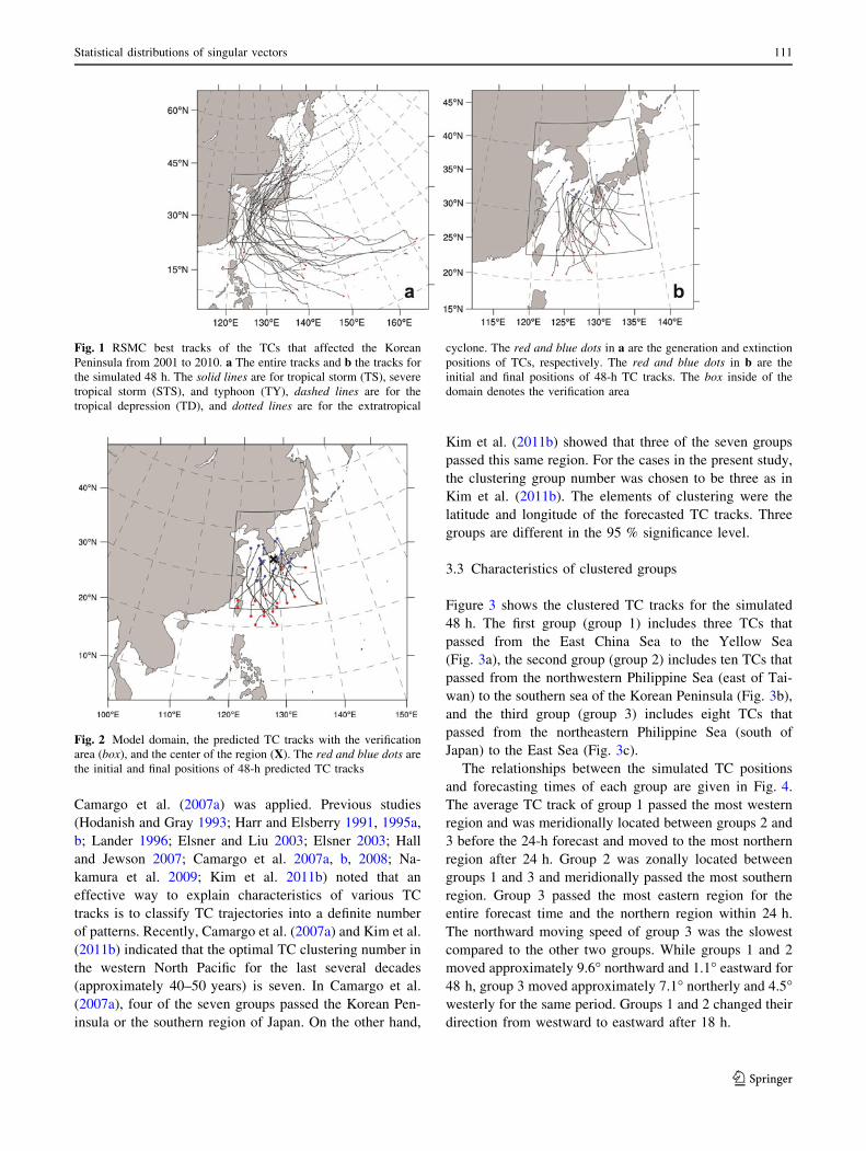
The entire RSMC best tracks for the chosen TCs are
shown in Fig. 1a and the 48-h tracks in Fig. 1b. Most of the
TCs generated within 5�–25�N and 120�–170�E passed
through the region of 120�–140� E over 30�N and disap-
peared or transformed into extratropical cyclones within
130�–180�E over 40�N. During the simulated 48 h, most of
the tracks started at the northern Philippine Sea and ended
at the Yellow Sea, East China Sea, or East Sea/Japan Sea.
Figure 2 shows the predicted TC tracks with the verifica-
tion region in the model domain. On average, the predicted
track error at the verification time was 182 km. To deter-
mine the predicted TC track (i.e., position of the TC cen-
ter), the TC tracking method by Kim and Kim (2010) was
used.
3.2 Clustering of the cases
Because the influence of TCs on the Korean Peninsula is
determined mostly by TC tracks, statistical TESV distri-
butions depending on TC tracks are evaluated. To deter-
mine the characteristics of TCs according to track, the
clustering analysis based on a regression mixture model by
Table 1 List of TCs affecting the Korean Peninsula during the past 10 years
No. Name TC number Initial time Class Lat (N) Lon (E) Press (hPa) Group
1 RAMMASUN 200205 2002070318 5 25.6 124.9 945 1
2 KALMAEGI 200807 2008071806 3 26.1 120.5 994 1
3 MALOU 201009 2010090412 3 27.0 127.0 998 1
4 LINFA 200304 2003052818 3 20.9 125.3 992 2
5 ETAU 200310 2003080612 5 23.9 128.8 955 2
6 MAEMI 200314 2003091006 5 24.0 126.6 910 2
7 MINDULLE 200407 2004070118 4 23.9 120.5 980 2
8 MEGI 200415 2004081618 3 21.2 128.8 992 2
9 SONGDA 200418 2004090418 5 25.1 129.7 925 2
10 EWINIAR 200603 2006070718 5 22.5 126.5 950 2
11 SHANSHAN 200613 2006091506 5 22.1 124.0 935 2
12 MAN-YI 200704 2007071200 5 21.0 129.2 930 2
13 NARI 200711 2007091400 5 24.4 129.4 960 2
14 PABUK 200111 2001081906 5 26.3 133.7 960 3
15 FENGSHEN 200209 2002072412 5 28.7 137.7 965 3
16 RUSA 200215 2002082900 5 27.6 131.3 950 3
17 NAMTHEUN 200410 2004073006 5 31.8 137.2 965 3
18 CHABA 200416 2004082806 5 27.4 133.6 935 3
19 NABI 200514 2005090400 5 24.8 132.2 940 3
20 WUKONG 200610 2006081718 3 32.0 131.1 980 3
21 USAGI 200705 2007073118 5 24.2 137.9 950 3
22 NAKRI 200208 2002071112 3 25.6 126.3 990 –
23 SOUDELOR 200306 2003061706 4 20.7 123.2 975 –
24 DIANMU 201004 2010080812 3 23.6 124.9 994 –
25 KOMPASU 201007 2010083012 4 23.7 131.2 980 –
The ‘‘Class’’ column represents the TC type [tropical storm (TS, 3), severe tropical storm (STS, 4), and Typhoon (TY, 5)], ‘‘Press’’ represents the
central pressure of the TC by RSMC best track information, ‘‘Group’’ represents the clustered group number of each case. The 22nd to 25th TCs
were excluded from the study
110 S.-Y. Park et al.
123
Camargo et al. (2007a) was applied. Previous studies
(Hodanish and Gray 1993; Harr and Elsberry 1991, 1995a,
b; Lander 1996; Elsner and Liu 2003; Elsner 2003; Hall
and Jewson 2007; Camargo et al. 2007a, b, 2008; Na-
kamura et al. 2009; Kim et al. 2011b) noted that an
effective way to explain characteristics of various TC
tracks is to classify TC trajectories into a definite number
of patterns. Recently, Camargo et al. (2007a) and Kim et al.
(2011b) indicated that the optimal TC clustering number in
the western North Pacific for the last several decades
(approximately 40–50 years) is seven. In Camargo et al.
(2007a), four of the seven groups passed the Korean Pen-
insula or the southern region of Japan. On the other hand,
Kim et al. (2011b) showed that three of the seven groups
passed this same region. For the cases in the present study,
the clustering group number was chosen to be three as in
Kim et al. (2011b). The elements of clustering were the
latitude and longitude of the forecasted TC tracks. Three
groups are different in the 95 % significance level.
3.3 Characteristics of clustered groups
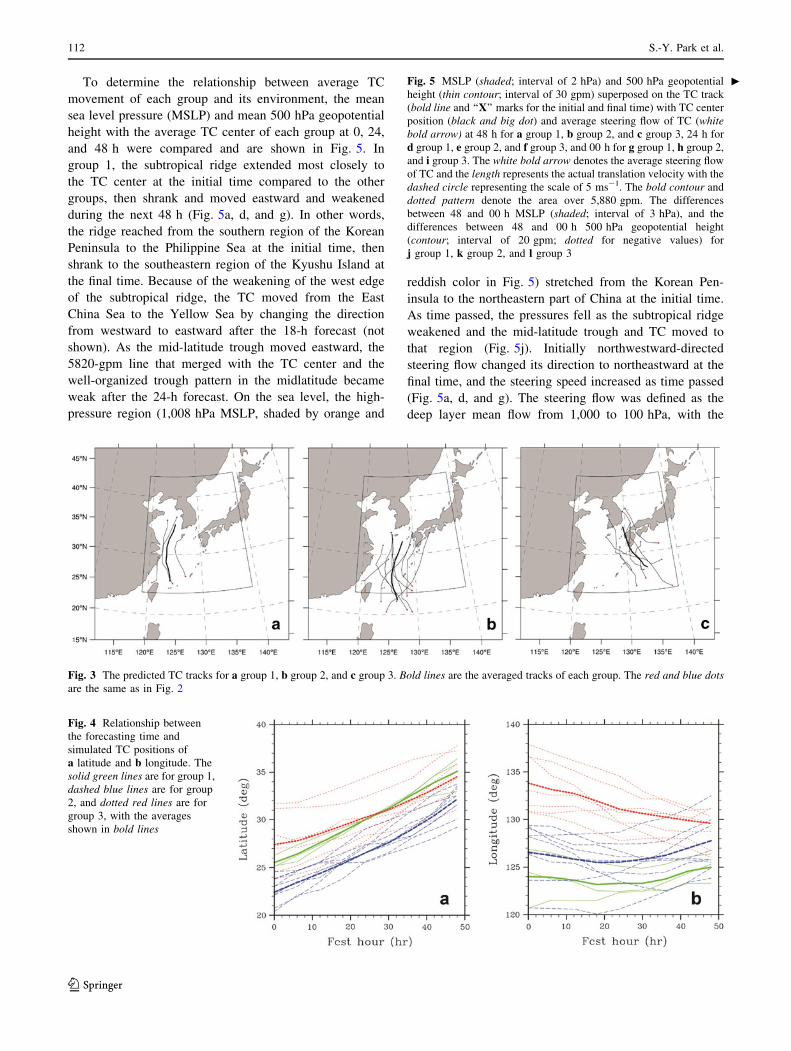
Figure 3 shows the clustered TC tracks for the simulated
48 h. The first group (group 1) includes three TCs that
passed from the East China Sea to the Yellow Sea
(Fig. 3a), the second group (group 2) includes ten TCs that
passed from the northwestern Philippine Sea (east of Tai-
wan) to the southern sea of the Korean Peninsula (Fig. 3b),
and the third group (group 3) includes eight TCs that
passed from the northeastern Philippine Sea (south of
Japan) to the East Sea (Fig. 3c).
The relationships between the simulated TC positions
and forecasting times of each group are given in Fig. 4.
The average TC track of group 1 passed the most western
region and was meridionally located between groups 2 and
3 before the 24-h forecast and moved to the most northern
region after 24 h. Group 2 was zonally located between
groups 1 and 3 and meridionally passed the most southern
region. Group 3 passed the most eastern region for the
entire forecast time and the northern region within 24 h.
The northward moving speed of group 3 was the slowest
compared to the other two groups. While groups 1 and 2
moved approximately 9.6� northward and 1.1� eastward for
48 h, group 3 moved approximately 7.1� northerly and 4.5�westerly for the same period. Groups 1 and 2 changed their
direction from westward to eastward after 18 h.
Fig. 1 RSMC best tracks of the TCs that affected the Korean
Peninsula from 2001 to 2010. a The entire tracks and b the tracks for
the simulated 48 h. The solid lines are for tropical storm (TS), severe
tropical storm (STS), and typhoon (TY), dashed lines are for the
tropical depression (TD), and dotted lines are for the extratropical
cyclone. The red and blue dots in a are the generation and extinction
positions of TCs, respectively. The red and blue dots in b are the
initial and final positions of 48-h TC tracks. The box inside of the
domain denotes the verification area
Fig. 2 Model domain, the predicted TC tracks with the verification
area (box), and the center of the region (X). The red and blue dots are
the initial and final positions of 48-h predicted TC tracks
Statistical distributions of singular vectors 111
123
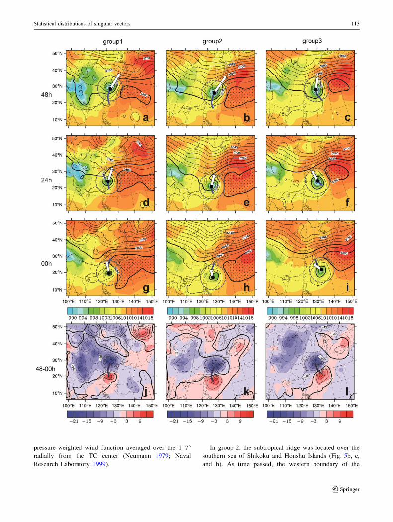
To determine the relationship between average TC
movement of each group and its environment, the mean
sea level pressure (MSLP) and mean 500 hPa geopotential
height with the average TC center of each group at 0, 24,
and 48 h were compared and are shown in Fig. 5. In
group 1, the subtropical ridge extended most closely to
the TC center at the initial time compared to the other
groups, then shrank and moved eastward and weakened
during the next 48 h (Fig. 5a, d, and g). In other words,
the ridge reached from the southern region of the Korean
Peninsula to the Philippine Sea at the initial time, then
shrank to the southeastern region of the Kyushu Island at
the final time. Because of the weakening of the west edge
of the subtropical ridge, the TC moved from the East
China Sea to the Yellow Sea by changing the direction
from westward to eastward after the 18-h forecast (not
shown). As the mid-latitude trough moved eastward, the
5820-gpm line that merged with the TC center and the
well-organized trough pattern in the midlatitude became
weak after the 24-h forecast. On the sea level, the high-
pressure region (1,008 hPa MSLP, shaded by orange and
reddish color in Fig. 5) stretched from the Korean Pen-
insula to the northeastern part of China at the initial time.
As time passed, the pressures fell as the subtropical ridge
weakened and the mid-latitude trough and TC moved to
that region (Fig. 5j). Initially northwestward-directed
steering flow changed its direction to northeastward at the
final time, and the steering speed increased as time passed
(Fig. 5a, d, and g). The steering flow was defined as the
deep layer mean flow from 1,000 to 100 hPa, with the
Fig. 3 The predicted TC tracks for a group 1, b group 2, and c group 3. Bold lines are the averaged tracks of each group. The red and blue dotsare the same as in Fig. 2
Fig. 4 Relationship between
the forecasting time and
simulated TC positions of
a latitude and b longitude. The
solid green lines are for group 1,
dashed blue lines are for group
2, and dotted red lines are for
group 3, with the averages
shown in bold lines
Fig. 5 MSLP (shaded; interval of 2 hPa) and 500 hPa geopotential
height (thin contour; interval of 30 gpm) superposed on the TC track
(bold line and ‘‘X’’ marks for the initial and final time) with TC center
position (black and big dot) and average steering flow of TC (whitebold arrow) at 48 h for a group 1, b group 2, and c group 3, 24 h for
d group 1, e group 2, and f group 3, and 00 h for g group 1, h group 2,
and i group 3. The white bold arrow denotes the average steering flow
of TC and the length represents the actual translation velocity with the
dashed circle representing the scale of 5 ms-1. The bold contour and
dotted pattern denote the area over 5,880 gpm. The differences
between 48 and 00 h MSLP (shaded; interval of 3 hPa), and the
differences between 48 and 00 h 500 hPa geopotential height
(contour; interval of 20 gpm; dotted for negative values) for
j group 1, k group 2, and l group 3
c
112 S.-Y. Park et al.
123
pressure-weighted wind function averaged over the 1–7�radially from the TC center (Neumann 1979; Naval
Research Laboratory 1999).
In group 2, the subtropical ridge was located over the
southern sea of Shikoku and Honshu Islands (Fig. 5b, e,
and h). As time passed, the western boundary of the
Statistical distributions of singular vectors 113
123
subtropical ridge moved eastward. Compared to group 1,
the location of the subtropical ridge did not change sig-
nificantly. Similar to group 1, the TC recurved along the
subtropical ridge, the mid-latitude trough moved eastward,
and the 5,820-gpm line merged with the TC center after the
24-h forecast. The well-organized mid-latitude system at
the initial time was well maintained during the 48-h fore-
cast. Different from the group 1, the high-pressure pattern
was shown over Manchuria during the entire forecast
period even though it was weakened as the subtropical
ridge shrank toward east (Fig. 5k). The steering flow of
group 2 shows similar pattern to that of group 1, with more
increasing speed. Because the magnitude of steering flow
during 24–48 h (2.99 ms-1) was larger than that during
00–24 h (1.76 ms-1), the recurving of TCs was enhanced
during the later 24 h (Fig. 5b, e, and h).
In group 3, the subtropical ridge moved to the northeastern
region and shrank as time passed (Fig. 5c, f, and i). Different
from groups 1 and 2, the subtropical ridge was located in the
northern area of the TC center during the entire forecast
period, and the mid-latitude trough moved very slowly
toward the east (Fig. 5l). The axis of the trough reached from
Manchuria to mid-eastern China. Initially northwestward-
directed steering flow changed its direction to northward at
the final time, and the steering speed did not increase much as
time passed (Fig. 5c, f, and i). The locations of the sub-
tropical ridge and mid-latitude trough and steering flow
indicated that the TC steering was weak for TCs in this group.
The 5,820-gpm line was merged with the TC at 42 h (not
shown). Cyclone barely reaches latitude of ridge axis.
3.4 Characteristics of normalized average TESVs
3.4.1 Horizontal structures
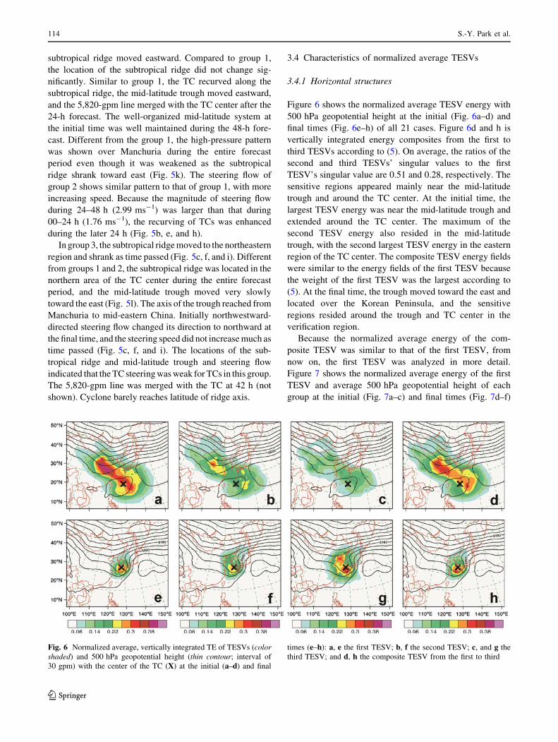
Figure 6 shows the normalized average TESV energy with
500 hPa geopotential height at the initial (Fig. 6a–d) and
final times (Fig. 6e–h) of all 21 cases. Figure 6d and h is
vertically integrated energy composites from the first to
third TESVs according to (5). On average, the ratios of the
second and third TESVs’ singular values to the first
TESV’s singular value are 0.51 and 0.28, respectively. The
sensitive regions appeared mainly near the mid-latitude
trough and around the TC center. At the initial time, the
largest TESV energy was near the mid-latitude trough and
extended around the TC center. The maximum of the
second TESV energy also resided in the mid-latitude
trough, with the second largest TESV energy in the eastern
region of the TC center. The composite TESV energy fields
were similar to the energy fields of the first TESV because
the weight of the first TESV was the largest according to
(5). At the final time, the trough moved toward the east and
located over the Korean Peninsula, and the sensitive
regions resided around the trough and TC center in the
verification region.
Because the normalized average energy of the com-
posite TESV was similar to that of the first TESV, from
now on, the first TESV was analyzed in more detail.
Figure 7 shows the normalized average energy of the first
TESV and average 500 hPa geopotential height of each
group at the initial (Fig. 7a–c) and final times (Fig. 7d–f)
Fig. 6 Normalized average, vertically integrated TE of TESVs (colorshaded) and 500 hPa geopotential height (thin contour; interval of
30 gpm) with the center of the TC (X) at the initial (a–d) and final
times (e–h): a, e the first TESV; b, f the second TESV; c, and g the
third TESV; and d, h the composite TESV from the first to third
114 S.-Y. Park et al.
123
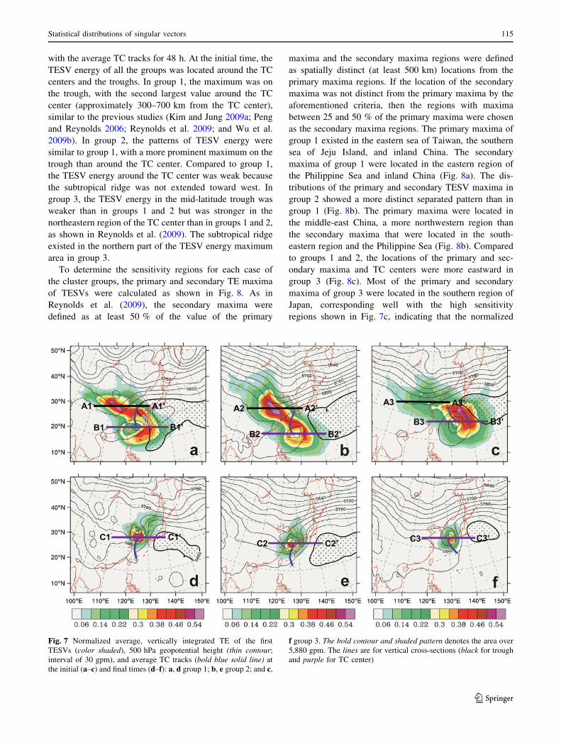
with the average TC tracks for 48 h. At the initial time, the
TESV energy of all the groups was located around the TC
centers and the troughs. In group 1, the maximum was on
the trough, with the second largest value around the TC
center (approximately 300–700 km from the TC center),
similar to the previous studies (Kim and Jung 2009a; Peng
and Reynolds 2006; Reynolds et al. 2009; and Wu et al.
2009b). In group 2, the patterns of TESV energy were
similar to group 1, with a more prominent maximum on the
trough than around the TC center. Compared to group 1,
the TESV energy around the TC center was weak because
the subtropical ridge was not extended toward west. In
group 3, the TESV energy in the mid-latitude trough was
weaker than in groups 1 and 2 but was stronger in the
northeastern region of the TC center than in groups 1 and 2,
as shown in Reynolds et al. (2009). The subtropical ridge
existed in the northern part of the TESV energy maximum
area in group 3.
To determine the sensitivity regions for each case of
the cluster groups, the primary and secondary TE maxima
of TESVs were calculated as shown in Fig. 8. As in
Reynolds et al. (2009), the secondary maxima were
defined as at least 50 % of the value of the primary
maxima and the secondary maxima regions were defined
as spatially distinct (at least 500 km) locations from the
primary maxima regions. If the location of the secondary
maxima was not distinct from the primary maxima by the
aforementioned criteria, then the regions with maxima
between 25 and 50 % of the primary maxima were chosen
as the secondary maxima regions. The primary maxima of
group 1 existed in the eastern sea of Taiwan, the southern
sea of Jeju Island, and inland China. The secondary
maxima of group 1 were located in the eastern region of
the Philippine Sea and inland China (Fig. 8a). The dis-
tributions of the primary and secondary TESV maxima in
group 2 showed a more distinct separated pattern than in
group 1 (Fig. 8b). The primary maxima were located in
the middle-east China, a more northwestern region than
the secondary maxima that were located in the south-
eastern region and the Philippine Sea (Fig. 8b). Compared
to groups 1 and 2, the locations of the primary and sec-
ondary maxima and TC centers were more eastward in
group 3 (Fig. 8c). Most of the primary and secondary
maxima of group 3 were located in the southern region of
Japan, corresponding well with the high sensitivity
regions shown in Fig. 7c, indicating that the normalized
Fig. 7 Normalized average, vertically integrated TE of the first
TESVs (color shaded), 500 hPa geopotential height (thin contour;
interval of 30 gpm), and average TC tracks (bold blue solid line) at
the initial (a–c) and final times (d–f): a, d group 1; b, e group 2; and c,
f group 3. The bold contour and shaded pattern denotes the area over
5,880 gpm. The lines are for vertical cross-sections (black for trough
and purple for TC center)
Statistical distributions of singular vectors 115
123
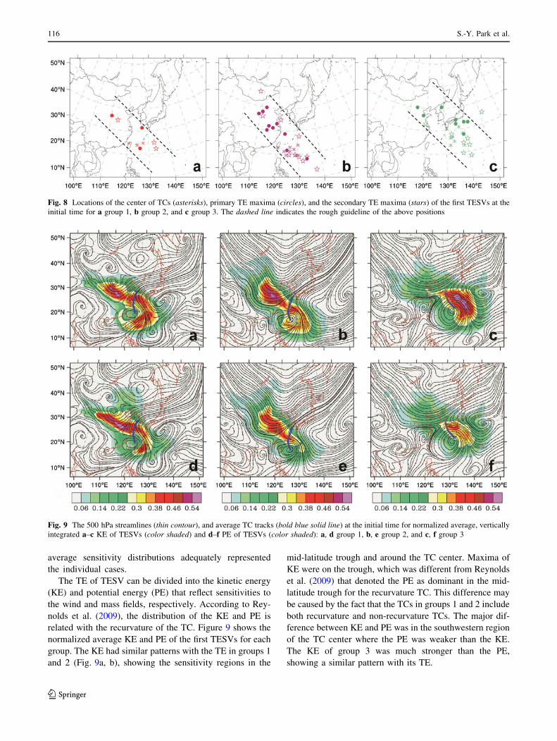
average sensitivity distributions adequately represented
the individual cases.
The TE of TESV can be divided into the kinetic energy
(KE) and potential energy (PE) that reflect sensitivities to
the wind and mass fields, respectively. According to Rey-
nolds et al. (2009), the distribution of the KE and PE is
related with the recurvature of the TC. Figure 9 shows the
normalized average KE and PE of the first TESVs for each
group. The KE had similar patterns with the TE in groups 1
and 2 (Fig. 9a, b), showing the sensitivity regions in the
mid-latitude trough and around the TC center. Maxima of
KE were on the trough, which was different from Reynolds
et al. (2009) that denoted the PE as dominant in the mid-
latitude trough for the recurvature TC. This difference may
be caused by the fact that the TCs in groups 1 and 2 include
both recurvature and non-recurvature TCs. The major dif-
ference between KE and PE was in the southwestern region
of the TC center where the PE was weaker than the KE.
The KE of group 3 was much stronger than the PE,
showing a similar pattern with its TE.
Fig. 9 The 500 hPa streamlines (thin contour), and average TC tracks (bold blue solid line) at the initial time for normalized average, vertically
integrated a–c KE of TESVs (color shaded) and d–f PE of TESVs (color shaded): a, d group 1, b, e group 2, and c, f group 3
Fig. 8 Locations of the center of TCs (asterisks), primary TE maxima (circles), and the secondary TE maxima (stars) of the first TESVs at the
initial time for a group 1, b group 2, and c group 3. The dashed line indicates the rough guideline of the above positions
116 S.-Y. Park et al.
123
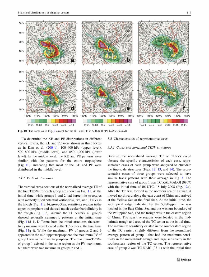
To determine the KE and PE distributions in different
vertical levels, the KE and PE were shown in three levels
as in Kim et al. (2004b): 100–400 hPa (upper level),
500–800 hPa (middle level), and 850–1,000 hPa (lower
level). In the middle level, the KE and PE patterns were
similar with the patterns for the entire troposphere
(Fig. 10), indicating that most of the KE and PE were
distributed in the middle level.
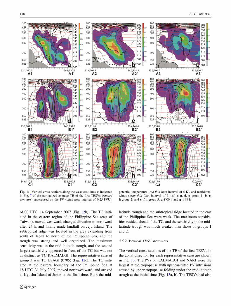
3.4.2 Vertical structures
The vertical cross-sections of the normalized average TE of
the first TESVs for each group are shown in Fig. 11. At the
initial time, while groups 1 and 2 had baroclinic structures
with westerly tilted potential vorticities (PVs) and TESVs in
the trough (Fig. 11a, b), group 3 had sensitivity regions in the
upper troposphere and showed much weaker baroclinicity in
the trough (Fig. 11c). Around the TC centers, all groups
showed generally symmetric patterns at the initial time
(Fig. 11d–f). Different from the initial structures, the sensi-
tivity maxima were located in the TC center at the final time
(Fig. 11g–i). While the maximum PV of groups 2 and 3
appeared in the mid-upper troposphere, the maximum PV of
group 1 was in the lower troposphere. The maximum TESVs
of group 1 existed in the same region as the PV maximum,
but there were two maxima in groups 2 and 3.
3.5 Characteristics of representative cases
3.5.1 Cases and horizontal TESV structures
Because the normalized average TE of TESVs could
obscure the specific characteristics of each case, repre-
sentative cases of each group were analyzed to elucidate
the fine-scale structures (Figs. 12, 13, and 14). The repre-
sentative cases of three groups were selected to have
similar track patterns with their average in Fig. 3. The
representative case of group 1 was TC KALMAEGI (0807)
with the initial time of 06 UTC, 18 July 2008 (Fig. 12a).
After the TC was formed in the northern sea of Taiwan, it
moved northward along the east coast of China and arrived
at the Yellow Sea at the final time. At the initial time, the
subtropical ridge indicated by the 5,880-gpm line was
located in the East China Sea and the western boundary of
the Philippine Sea, and the trough was in the eastern region
of China. The sensitive regions were located in the mid-
latitude trough and around the TC center at the initial time.
The maximum sensitivity existed in the southeastern region
of the TC center, slightly different from the normalized
average pattern of group 1 that had the maximum sensi-
tivity in the mid-latitude trough and large sensitivity in the
southeastern region of the TC center. The representative
case of group 2 was TC NARI (0711) with the initial time
Fig. 10 The same as in Fig. 9 except for the KE and PE in 500–800 hPa (color shaded)
Statistical distributions of singular vectors 117
123
of 00 UTC, 14 September 2007 (Fig. 12b). The TC initi-
ated in the eastern region of the Philippine Sea (east of
Taiwan), moved westward, changed direction to northward
after 24 h, and finally made landfall on Jeju Island. The
subtropical ridge was located in the area extending from
south of Japan to north of the Philippine Sea, and the
trough was strong and well organized. The maximum
sensitivity was in the mid-latitude trough, and the second
largest sensitivity appeared in front of the TC but was not
as distinct as TC KALMAEGI. The representative case of
group 3 was TC USAGI (0705) (Fig. 12c). The TC initi-
ated at the eastern boundary of the Philippine Sea at
18 UTC, 31 July 2007, moved northwestward, and arrived
at Kyushu Island of Japan at the final time. Both the mid-
latitude trough and the subtropical ridge located in the east
of the Philippine Sea were weak. The maximum sensitiv-
ities resided ahead of the TC, and the sensitivity in the mid-
latitude trough was much weaker than those of groups 1
and 2.
3.5.2 Vertical TESV structures
The vertical cross-sections of the TE of the first TESVs in
the zonal direction for each representative case are shown
in Fig. 13. The PVs of KALMAEGI and NARI were the
largest at the tropopause with upshear-tilted PV intrusions
caused by upper tropopause folding under the mid-latitude
trough at the initial time (Fig. 13a, b). The TESVs had also
Fig. 11 Vertical cross-sections along the west–east lines as indicated
in Fig. 7 of the normalized average TE of the first TESVs (shadedcontours) superposed on the PV (thick line; interval of 0.25 PVU),
potential temperature (red thin line; interval of 5 K), and meridional
winds (gray thin line; interval of 3 ms-1): a, d, g group 1; b, e,
h group 2; and c, f, i group 3. a–f 00 h and g–i 48 h
118 S.-Y. Park et al.
123
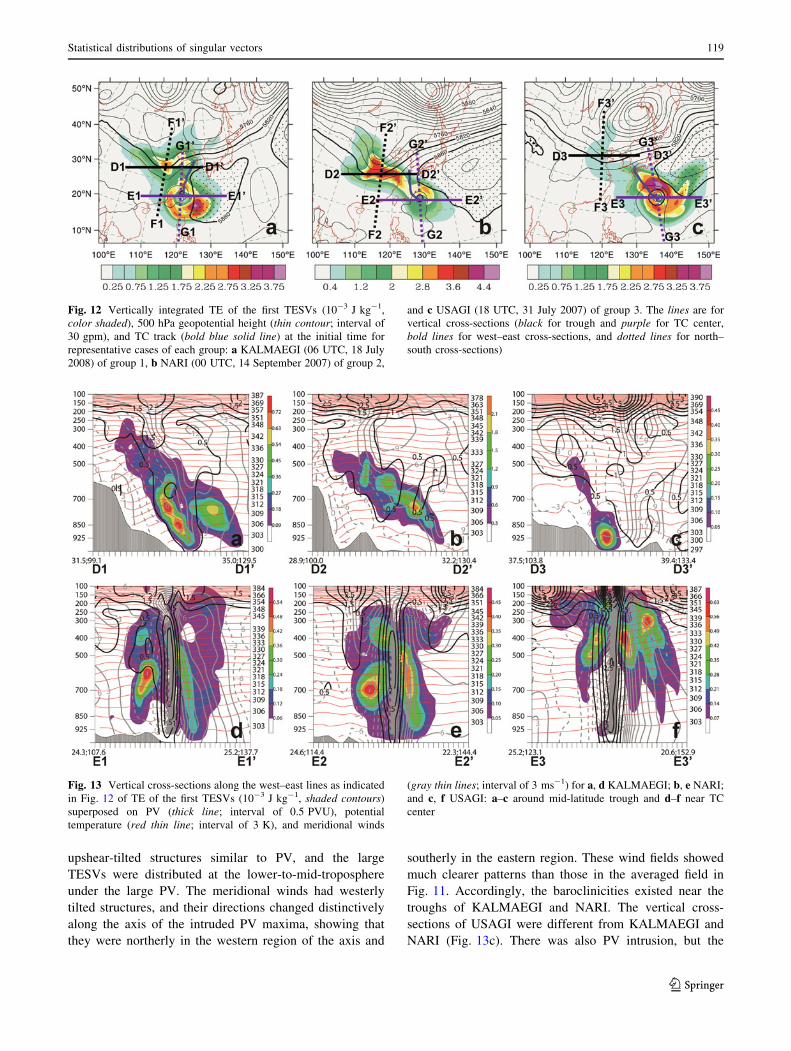
upshear-tilted structures similar to PV, and the large
TESVs were distributed at the lower-to-mid-troposphere
under the large PV. The meridional winds had westerly
tilted structures, and their directions changed distinctively
along the axis of the intruded PV maxima, showing that
they were northerly in the western region of the axis and
southerly in the eastern region. These wind fields showed
much clearer patterns than those in the averaged field in
Fig. 11. Accordingly, the baroclinicities existed near the
troughs of KALMAEGI and NARI. The vertical cross-
sections of USAGI were different from KALMAEGI and
NARI (Fig. 13c). There was also PV intrusion, but the
Fig. 12 Vertically integrated TE of the first TESVs (10-3 J kg-1,
color shaded), 500 hPa geopotential height (thin contour; interval of
30 gpm), and TC track (bold blue solid line) at the initial time for
representative cases of each group: a KALMAEGI (06 UTC, 18 July
2008) of group 1, b NARI (00 UTC, 14 September 2007) of group 2,
and c USAGI (18 UTC, 31 July 2007) of group 3. The lines are for
vertical cross-sections (black for trough and purple for TC center,
bold lines for west–east cross-sections, and dotted lines for north–
south cross-sections)
Fig. 13 Vertical cross-sections along the west–east lines as indicated
in Fig. 12 of TE of the first TESVs (10-3 J kg-1, shaded contours)
superposed on PV (thick line; interval of 0.5 PVU), potential
temperature (red thin line; interval of 3 K), and meridional winds
(gray thin lines; interval of 3 ms-1) for a, d KALMAEGI; b, e NARI;
and c, f USAGI: a–c around mid-latitude trough and d–f near TC
center
Statistical distributions of singular vectors 119
123
upshear-tilted structure was weaker than that of KAL-
MAEGI and NARI. The largest TESV energy was not very
tilted and was located in the western region of 0.5 PVU in
the lower troposphere. The meridional wind was also not
tilted.
Around the TC center for all three cases, the PVs,
TESVs, and meridional winds had nearly symmetric
structures (Fig. 13d–f). The PVs were the largest at the TC
center and were not tilted. The TESV maxima of KAL-
MAEGI and NARI were at the mid-troposphere, showing
asymmetry in detailed structures: maxima of TESVs at the
western region of the TC center were larger than at the
eastern region of the TC center and had oval shapes tilted
to the TC center, different from those in the eastern region
(Fig. 13d, e). For USAGI, the maximum region appeared at
the upper troposphere, different from groups 1 and 2
(Fig. 13f).
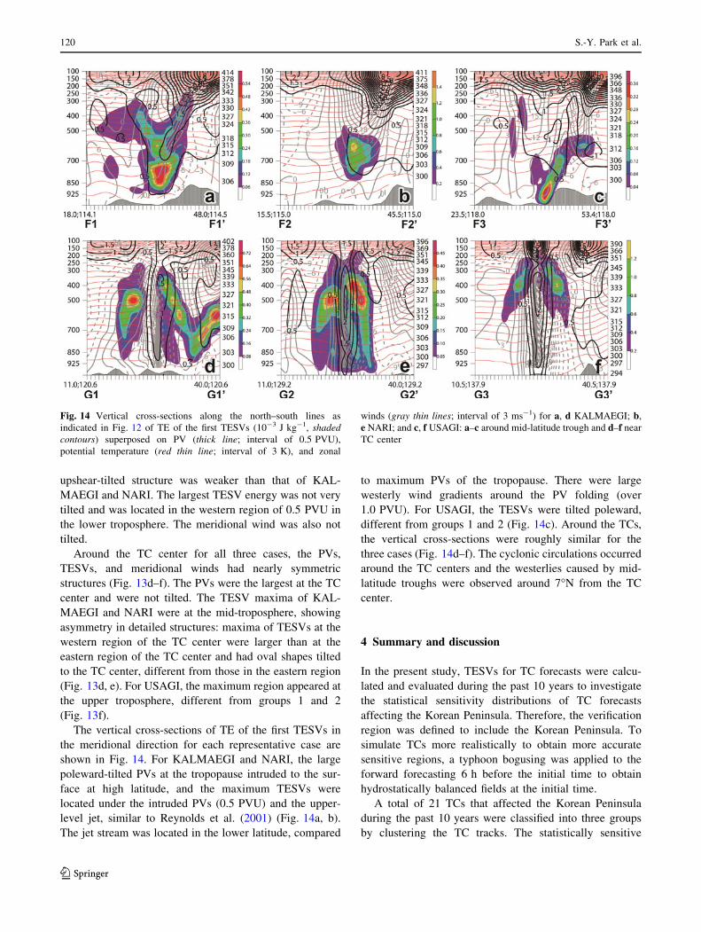
The vertical cross-sections of TE of the first TESVs in
the meridional direction for each representative case are
shown in Fig. 14. For KALMAEGI and NARI, the large
poleward-tilted PVs at the tropopause intruded to the sur-
face at high latitude, and the maximum TESVs were
located under the intruded PVs (0.5 PVU) and the upper-
level jet, similar to Reynolds et al. (2001) (Fig. 14a, b).
The jet stream was located in the lower latitude, compared
to maximum PVs of the tropopause. There were large
westerly wind gradients around the PV folding (over
1.0 PVU). For USAGI, the TESVs were tilted poleward,
different from groups 1 and 2 (Fig. 14c). Around the TCs,
the vertical cross-sections were roughly similar for the
three cases (Fig. 14d–f). The cyclonic circulations occurred
around the TC centers and the westerlies caused by mid-
latitude troughs were observed around 7�N from the TC
center.
4 Summary and discussion
In the present study, TESVs for TC forecasts were calcu-
lated and evaluated during the past 10 years to investigate
the statistical sensitivity distributions of TC forecasts
affecting the Korean Peninsula. Therefore, the verification
region was defined to include the Korean Peninsula. To
simulate TCs more realistically to obtain more accurate
sensitive regions, a typhoon bogusing was applied to the
forward forecasting 6 h before the initial time to obtain
hydrostatically balanced fields at the initial time.
A total of 21 TCs that affected the Korean Peninsula
during the past 10 years were classified into three groups
by clustering the TC tracks. The statistically sensitive
Fig. 14 Vertical cross-sections along the north–south lines as
indicated in Fig. 12 of TE of the first TESVs (10-3 J kg-1, shadedcontours) superposed on PV (thick line; interval of 0.5 PVU),
potential temperature (red thin line; interval of 3 K), and zonal
winds (gray thin lines; interval of 3 ms-1) for a, d KALMAEGI; b,
e NARI; and c, f USAGI: a–c around mid-latitude trough and d–f near
TC center
120 S.-Y. Park et al.
123
regions of the TCs were mainly in the mid-latitude trough
and around the TC centers at the initial time. The three
groups had characteristic environmental conditions such as
subtropical highs and mid-latitude troughs. The first group
passed from the East China Sea to the Yellow Sea, the
second group passed from the northwestern Philippine Sea
(east of Taiwan) to the southern sea of the Korean Penin-
sula, and the third group passed from the northeastern
Philippine Sea (south of Japan) to the East Sea/Japan Sea.
Nearly half of the TCs (ten of 21 TCs) were included in the
second group.
The relationship between TC movement and its envi-
ronment was analyzed. Holland and Wang (1995) demon-
strated that the TC recurvature occurs through an unbroken
subtropical high at the initial time and is substantially
enhanced by a mid-latitude trough. Corresponding to
Holland and Wang (1995), the TCs in groups 1 and 2
moved along the boundary and changed direction by the
subtropical ridges. As the TCs moved northward and the
mid-latitude troughs moved eastward, the recurvature was
enhanced. The TCs had the maximum sensitive regions
located in the mid-latitude troughs and largely sensitive
regions around the TC center. However, depending on the
extension of subtropical ridge, the primary sensitive
regions were changed. Therefore, the group 2 has relatively
weak sensitive regions around the TC center compared to
group 1. Conversely, the TC steering was weak for TCs in
group 3, where the sensitive regions were located around
the TC center.
To understand the dynamic features associated with
TESV sensitivities near the TC centers and in the mid-
latitude troughs, the vertical structures were examined.
While the first and second groups had westerly tilted TESV
and PV structures associated with baroclinic environments
in the mid-latitude trough at the initial time, the third group
showed weak baroclinicity. In groups 1 and 2, the large
poleward-tilted PVs at the tropopause in the high latitude
intruded to the surface, and the maxima TESVs were
located under the intruded PVs (0.5 PVU) and the upper-
level jet, in agreement with Reynolds et al. (2001). The
symmetric patterns were distinct for all groups around the
TC centers at the final time, and the TESV maxima were
located at the center of the TC at the final time.
Even though some specific characteristics of individual
cases were different with those of the average fields, the
analysis of the representative TC cases showed that the
average pattern of the sensitivity regions and atmospheric
systems roughly demonstrated characteristics of individual
cases. Given the results in the present study, TCs moving
toward a fixed verification region over the Korean Penin-
sula have different sensitivity regions and structures
according to their moving tracks and the characteristic
environmental conditions. For group 1 TCs, adaptive
observations both in mid-latitude trough and around TC
center would be beneficial for TC forecasts affecting the
Korean Peninsula. While the adaptive observations near the
mid-latitude trough would be beneficial for group 2 TCs,
those around the TC center would be beneficial for group 3
TCs. Because the mid-latitude troughs approaching the
Korean Peninsula are mostly located in upstream regions in
mainland China, it is difficult to do adaptive observations
over those regions. Making use of satellite data efficiently
over those upstream regions would be beneficial for
adaptively observing TCs affecting the Korean Peninsula.
Acknowledgments The authors thank two anonymous reviewers
for their valuable comments. The authors thank Dr. In-Hyuk Kwon
and Prof. Hyung-Bin Cheong for providing the bogusing method for
the typhoon simulation. This study was supported by the Korea
Meteorological Administration Research and Development Program
under grant CATER 2012-2030.
Open Access This article is distributed under the terms of the
Creative Commons Attribution License which permits any use, dis-
tribution, and reproduction in any medium, provided the original
author(s) and the source are credited.
References
Buizza R (1994) Localization of optimal perturbations using a
projection operator. Q J R Meteor Soc 120:1647–1681
Buizza R, Montani A (1999) Targeting observations using singular
vectors. J Atmos Sci 56:2965–2985
Byun K-Y, Lee T-Y (2012) Remote effects of tropical cyclones on
heavy rainfall over the Korean peninsula statistical and composite
analysis. Tellus A 64:14983. doi:10.3402/tellusa.v64i0.14983
Camargo SJ, Robertson AW, Gaffney SJ, Smyth P, Ghil M (2007a)
Cluster analysis of typhoon tracks. Part I: general properties.
J Clim 20:3635–3653
Camargo SJ, Robertson AW, Gaffney SJ, Smyth P, Ghil M (2007b)
Cluster analysis of typhoon tracks. Part II: large-scale circulation
and ENSO. J Clim 20:3654–3676
Camargo SJ, Robertson AW, Barnston AG, Ghil M (2008) Clustering
of eastern North Pacific tropical cyclone tracks: ENSO and MJO
effects. Geochem Geophys Geosyst 9:Q06V05. doi:10.1029/
2007GC001861
Chen J-H, Peng MS, Reynolds CA, Wu C–C (2009) Interpretation of
tropical cyclone forecast sensitivity from the singular vector
perspective. J Atmos Sci 66:3383–3400
Dorst NM (2007) The National Hurricane Research Project: 50 years
of research, rough rides, and name changes. Bull Am Meteor Soc
88:1566–1588
Ehrendorfer M, Errico RM (1995) Mesoscale predictability and the
spectrum of optimal perturbations. J Atmos Sci 52:3475–3500
Elsner JB (2003) Tracking hurricanes. Bull Am Meteor Soc
84:353–356
Elsner JB, Liu KB (2003) Examining the ENSO–typhoon hypothesis.
Clim Res 25:43–54
Frank WM (1977a) The structure and energetics of the tropical
cyclone I: storm structure. Mon Weather Rev 105:1119–1135
Frank WM (1977b) The structure and energetics of the tropical
cyclone II: dynamics and energetics. Mon Weather Rev
105:1136–1150
Statistical distributions of singular vectors 121
123
Gelaro R, Langland RH, Rohaly GD, Rosmond TE (1999) An
assessment of the singular-vector approach to targeted observing
using the FASTEX dataset. Q J R Meteor Soc 125:3299–3327
Hall TM, Jewson S (2007) Statistical modelling of North Atlantic
tropical cyclone tracks. Tellus 59A:486–498
Harr PA, Elsberry RL (1991) Tropical cyclone track characteristics as
a function of large-scale circulation anomalies. Mon Weather
Rev 119:1448–1468
Harr PA, Elsberry RL (1995a) Large-scale circulation variability over
the tropical western North Pacific. Part I: spatial patterns and
tropical cyclone characteristics. Mon Weather Rev 123:1225–1246
Harr PA, Elsberry RL (1995b) Large-scale circulation variability over
the tropical western North Pacific. Part II: persistence and
transition characteristics. Mon Weather Rev 123:1247–1268
Ho C-H, Baik J-J, Kim J-H, Gong D-Y, Sui C-H (2004) Interdecadal
changes in summertime typhoon tracks. J Clim 17:1767–1776
Hodanish S, Gray WM (1993) An observational analysis of tropical
cyclone recurvature. Mon Weather Rev 121:2665–2689
Holland GJ, Wang Y (1995) Baroclinic dynamics of simulated
tropical cyclone recurvature. J Atmos Sci 52:410–426
Jung B-J, Kim HM, Zhang F, Wu C-C (2012) Effect of targeted
dropsonde observations and best track data on the track forecasts
of Typhoon Sinlaku (2008) using an Ensemble Kalman Filter.
Tellus A 64:14984. doi:10.3402/tellusa.v64i0.14984
Kim HM, Jung B-J (2006) Adjoint-based forecast sensitivities of
Typhoon Rusa. Geophys Res Lett 33:L21813. doi:10.1029/
2006GL027289
Kim HM, Jung B-J (2009a) Singular vector structure and evolution of
a recurving tropical cyclone. Mon Weather Rev 137:505–524
Kim HM, Jung B-J (2009b) Influence of moist physics and norms on
singular vectors for a tropical cyclone. Mon Weather Rev
137:525–543
Kim J, Kim HM (2010) Development of a tropical cyclone tracker
and application to tropical cyclones occurred in 2008 in North
western Pacific. Abstract A41B-0070 presented at 2010 Fall
Meeting, AGU, San Francisco, California, 13–17 Dec
Kim HM, Morgan MC (2002) Dependence of singular vector
structure and evolution on the choice of norm. J Atmos Sci
59:3099–3116
Kim HM, Morgan MC, Morss RE (2004a) Evolution of analysis error
and adjoint-based sensitivities: implications for adaptive obser-
vations. J Atmos Sci 61:795–812
Kim HM, Youn Y-H, Chung H-S (2004b) Potential vorticity thinking
as an aid to understanding midlatitude weather systems. J Korean
Meteor Soc 40:633–647
Kim HM, Kim S-M, Jung B-J (2011a) Real-time adaptive observation
guidance using singular vectors for Typhoon Jangmi (200815) in
T-PARC 2008. Weather Forecast 26:634–649
Kim H-S, Kim J-H, Ho C-H, Chu P-S (2011b) Pattern classification of
typhoon tracks using the fuzzy c-means clustering method.
J Clim 24:488–508
Kurihara Y, Tuleya RE (1974) Structure of a tropical cyclone
developed in a three-dimensional numerical simulation model.
J Atmos Sci 31:893–919
Kwon I-H, Cheong H-B (2010) Tropical cyclone initialization with a
spherical high-order filter and an idealized three-dimensional
bogus vortex. Mon Weather Rev 138:1344–1367
Kwon YC, Frank WM (2005) Dynamic instabilities of simulated
hurricane-like vortices and their impacts on the core structure of
hurricanes. Part I: dry experiments. J Atmos Sci 62:3955–3973
Kwon YC, Frank WM (2008) Dynamic instabilities of simulated
hurricane-like vortices and their impacts on the core structure of
hurricanes. Part II: moist experiments. J Atmos Sci 65:106–122
Lander MA (1996) Specific tropical cyclone track types and unusual
tropical cyclone motions associated with a reverse-oriented
monsoon trough in the western North Pacific. Weather Forecast
11:170–186
Lang STK, Jones SC, Leutbecher M, Peng MS, Reynolds CA (2012)
Sensitivity, structure, and dynamics of singular vectors associ-
ated with Hurricane Helene (2006). J Atmos Sci 69:675–694
Majumdar SJ, Aberson SD, Bishop CH, Buizza R, Peng MS,
Reynolds CA (2006) A comparison of adaptive observing
guidance for Atlantic tropical cyclones. Mon Weather Rev
134:2354–2372
Montani A, Thorpe AJ, Buizza R, Unden P (1999) Forecast skill of
the ECMWF model using targeted observations during FAS-
TEX. Q J R Meteor Soc 125:3219–3240
Nakamura J, Lall U, Kushnir Y, Camargo SJ (2009) Classifying North
Atlantic tropical cyclone tracks by mass moments. J Clim
22:5481–5494
National Typhoon Center (2011) Typhoon white book. Korean
Meteorological Administration, Korea, pp 224–225
Naval Research Laboratory (1999) Tropical cyclone forecasters’
reference guide. Chapter 4-1. Influences on tropical cyclone
motion. http://www.nrlmry.navy.mil/*chu/chap4/se100.htm.
Accessed 14 July 2012
Neumann CJ (1979) On the use of deep-layer-mean geopotential
height fields in statistical prediction of tropical cyclone motion.
In: 6th conference on probability and statistics in atmospheric
sciences. American Meteorological Society, Boston, pp 32–38
Palmer TN, Gelaro R, Barkmeijer J, Buizza R (1998) Singular
vectors, metrics, and adaptive observations. J Atmos Sci
55:633–653
Peng MS, Reynolds CA (2005) Double trouble for typhoon forecast-
ers. Geophys Res Lett 32:L02810. doi:10.1029/2004GL021680
Peng MS, Reynolds CA (2006) Sensitivity of tropical cyclone
forecasts as revealed by singular vectors. J Atmos Sci
63:2508–2528
Rappaport EN et al (2009) Advances and challenges at the National
Hurricane Center. Weather Forecast 24:395–419
Reynolds CA, Gelaro R, Rosmond R (2001) Relationship between
singular vectors and transient features in the background flow.
Q J R Meteor Soc 127:1731–1760
Reynolds CA, Peng MS, Chen J-H (2009) Recurving tropical
cyclones: singular vector sensitivity and downstream impact.
Mon Weather Rev 137:1320–1337
Wang Y (2002) Vortex Rossby Waves in a numerically simulated
tropical cyclone. Part II: the role in tropical cyclone structure and
intensity changes. J Atmos Sci 59:1239–1262
Wang Y, Holland GJ, Leslies LM (1993) Some baroclinic aspects of
tropical cyclone motion. In: Lighthill J, Emmanuel K, Holland G
(eds) Tropical cyclone disaster. Beijing University Press, China,
pp 280–285
Wu CC, Chen J-H, Lin P-H, Chou K-H (2007) Targeted observations
of tropical cyclone movement based on the adjoint-derived
sensitivity steering vector. J Atmos Sci 64:2611–2626
Wu CC, Chen S-G, Chen J-H, Chou K-H, Lin P-H (2009a) Interaction
of Typhoon Shanshan (2006) with the midlatitude trough from
both adjoint-derived sensitivity steering vector and potential
vorticity perspectives. Mon Weather Rev 137:852–862
Wu CC, Chen J-H, Majumdar SJ, Peng MS, Reynolds CA, Aberson
SD, Buizza R, Yamaguchi M, Chen S-G, Nakazawa T, Chou
K-H (2009b) Intercomparison of targeted observation guidance
for tropical cyclones in the Northwestern Pacific. Mon Weather
Rev 137:2471–2492
Zou X, Vandenberghe F, Pondeca M, Kuo Y-H (1997) Introduction to
adjoint techniques and the MM5 adjoint modeling system.
NCAR Technical Note NCAR/TN- 435STR, pp 110
122 S.-Y. Park et al.
123
![arXiv:1311.2657v5 [math.NA] 16 Nov 2017 · 2017. 11. 20. · 2 S. O’ROURKE, VAN VU, AND KE WANG the singular values and singular vectors. This problem has been discussed in virtu-ally](https://static.fdocuments.in/doc/165x107/60ccd420b4e4346a6d6d93c7/arxiv13112657v5-mathna-16-nov-2017-2017-11-20-2-s-oarourke-van-vu.jpg)


![Optimization Models [.1] Exercisespeople.eecs.berkeley.edu/~elghaoui/ExManual.pdfOPTIMIZATION MODELS EXERCISES CAMBRIDGE Contents 2.Vectors 4 3.Matrices 7 4.Symmetric matrices 11 5.Singular](https://static.fdocuments.in/doc/165x107/5fc0d32b1f9e393e246292a3/optimization-models-1-elghaouiexmanualpdf-optimization-models-exercises-cambridge.jpg)


