Statistical Data Analysis in R:a Short In-Depth Tutorial

George Ostrouchov , NCCS Vis Team and CSM Statistics & Data Sciences

March 28, 2007

George Ostrouchov , NCCS Vis Team and CSM Statistics & Data Sciences

March 28, 2007

2

CO2 Analysis in R: Tip of the Iceberg

• Same data set – high dimensional analysis• How does CO2 relate to other variables?

− Change over time− Altitude effects?− Do these change with humidity?− What about clouds?− So far we have a 5-D relationship.− Can we visualize 5-D?− What about 5-D density?! CO2 Exploratory Analysis in R:

• Preparing and reading data

• Lattice package for multivariate graphics

• Command line interface

Overview: R system for statistical computing

3

Selecting and Reading the Data

• Systematic sample:− Trend – years 1900, 1910, 1920, …, 1990− Seasonality – keep 12 mo in the selected

years− Select variables from the 128 available

• lon, lat, lev, year, month• CLDICE, CLDLIQ, CLOUD, CMFDQ,

CMFDQR, CO2_FFF, CO2_LND, CO2_OCN, CONCLD, RELHUM, LANDFRAC, OMEGA, T, U, PDELDRY

• ncdf package for reading NetCDF files• Write reader function• Output 14,376,960 by 20 matrix: x

− lon x lat x lev x year x month− 96 x 48 x 26 x 10 x 12 = 14,376,960

• R image: 3GB (8GB while constructing)• ~ 20 minutes on hawk50

Jan Feb Mar Apr May Jun Jul Aug Sep Oct Nov Dec

1900

1910

1920

1930

1940

1950

1960

1970

1980

1990

Each globe is lon x lat x lev (96 x 48 x 26) volumes.Each volume has 20 variables.

How does CO2 relate to other variables?• Change over time• Altitude effects?• Do these change with humidity?• What about clouds?• So far we have a 5-D relationship.• Can we visualize 5-D?• What about 5-D density?!

4

CO2_LND – Net CO2 Contribution from Land

% module load R

% R

. . .

> x <- getData(“/nfs/data/ost/climate.f14”, seq(1900,1990,10))

> require(lattice)

> histogram( ~ CO2_LND, x, nint=500)

J F M A M J J A S O N D

1900

1910

1920

1930

1940

1950

1960

1970

1980

1990

Each globe is lon x lat x lev (96 x 48 x 26) volumes.Each volume has 20 variables.

5

CO2_OCN – Net CO2 Contribution from Ocean

x <- getData(“/nfs/data/ost/climate.f14”, seq(1900,1990,10))

histogram( ~ CO2_LND, x, nint=500)

histogram( ~ CO2_OCN, x, nint=500)

6

CO2_FFF – Net CO2 Man Made Contribution

x <- getData(“/nfs/data/ost/climate.f14”, seq(1900,1990,10))

histogram( ~ CO2_LND, x, nint=500)

histogram( ~ CO2_OCN, x, nint=500)

histogram( ~ CO2_FFF, x, nint=500)

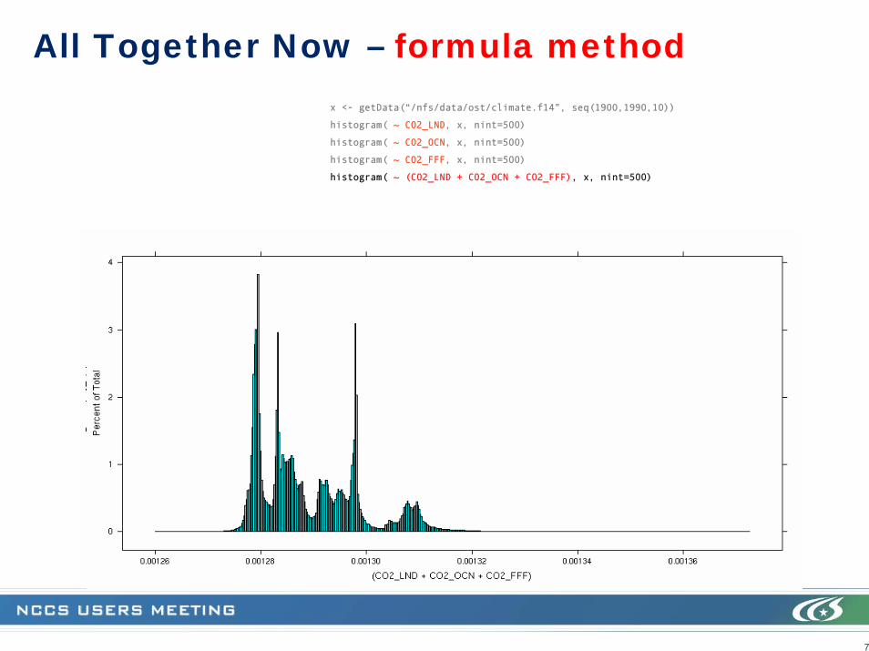
7

All Together Now – formula methodx <- getData(“/nfs/data/ost/climate.f14”, seq(1900,1990,10))

histogram( ~ CO2_LND, x, nint=500)

histogram( ~ CO2_OCN, x, nint=500)

histogram( ~ CO2_FFF, x, nint=500)

histogram( ~ (CO2_LND + CO2_OCN + CO2_FFF), x, nint=500)

8

Each Togetherx <- getData(“/nfs/data/ost/climate.f14”, seq(1900,1990,10))

histogram( ~ CO2_LND, x, nint=500)

histogram( ~ CO2_OCN, x, nint=500)

histogram( ~ CO2_FFF, x, nint=500)

histogram( ~ (CO2_LND + CO2_OCN + CO2_FFF), x, nint=500)

histogram( ~ CO2_LND + CO2_OCN + CO2_FFF, x, nint=200, layout=c(1,3))

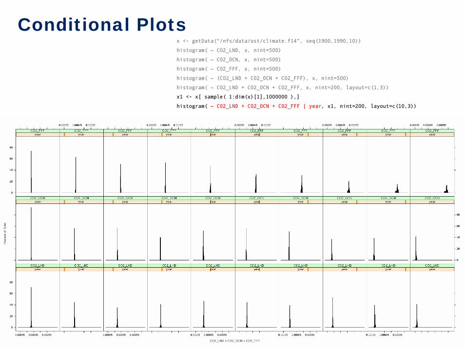
9

Conditional Plotsx <- getData(“/nfs/data/ost/climate.f14”, seq(1900,1990,10))

histogram( ~ CO2_LND, x, nint=500)

histogram( ~ CO2_OCN, x, nint=500)

histogram( ~ CO2_FFF, x, nint=500)

histogram( ~ (CO2_LND + CO2_OCN + CO2_FFF), x, nint=500)

histogram( ~ CO2_LND + CO2_OCN + CO2_FFF, x, nint=200, layout=c(1,3))

x1 <- x[ sample( 1:dim(x)[1],1000000 ),]

histogram( ~ CO2_LND + CO2_OCN + CO2_FFF | year, x1, nint=200, layout=c(10,3))

10

Scatter Plothistogram( ~ CO2_LND + CO2_OCN + CO2_FFF | year, x1, nint=200, layout=c(1,3) )

xyplot( CO2_FFF ~ (CO2_LND + CO2_OCN), x1 )

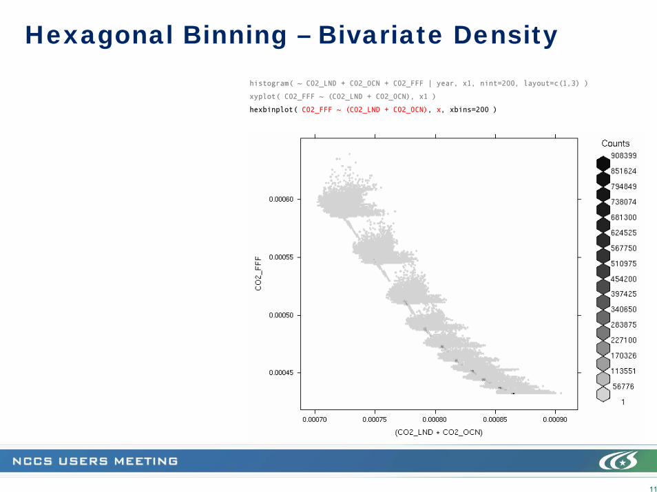
11

Hexagonal Binning – Bivariate Densityhistogram( ~ CO2_LND + CO2_OCN + CO2_FFF | year, x1, nint=200, layout=c(1,3) )

xyplot( CO2_FFF ~ (CO2_LND + CO2_OCN), x1 )

hexbinplot( CO2_FFF ~ (CO2_LND + CO2_OCN), x, xbins=200 )

12

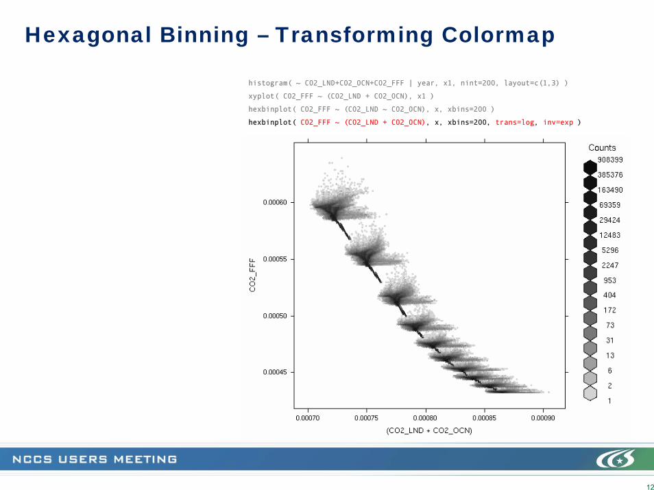
Hexagonal Binning – Transforming Colormap

histogram( ~ CO2_LND+CO2_OCN+CO2_FFF | year, x1, nint=200, layout=c(1,3) )

xyplot( CO2_FFF ~ (CO2_LND + CO2_OCN), x1 )

hexbinplot( CO2_FFF ~ (CO2_LND ~ CO2_OCN), x, xbins=200 )

hexbinplot( CO2_FFF ~ (CO2_LND + CO2_OCN), x, xbins=200, trans=log, inv=exp )

13

CO2 Sources 1900 to 1990: Shifting to Fossil Fuels

histogram( ~ CO2_LND + CO2_OCN + CO2_FFF | year, x1, nint=200, layout=c(1,3) )

xyplot( CO2_LND ~ CO2_OCN, x1 )

hexbinplot( CO2_FFF ~ (CO2_LND + CO2_OCN), x, xbins=200 )

hexbinplot( CO2_FFF ~ (CO2_LND + CO2_OCN), x, xbins=200, trans=log, inv=exp )

hexbinplot( CO2_FFF ~ (CO2_LND + CO2_OCN) | year, x, xbins=200, trans=log, inv=exp )

14

How does CO2 relate to other variables?• How does it change with time?• What are the CO2 seasonal effects?• How do the seasonal effects depend on

land fraction?• Does this dependence change with

humidity?• What about temperature?

hexbinplot( CO2_FFF ~ (CO2_LND + CO2_OCN) | year, x, xbins=200, trans=log, inv=exp )

hexbinplot( CO2_FFF ~ (CO2_LND + CO2_OCN) | lev, x, xbins=200, trans=log, inv=exp )

CO2 Sources by Altitude

15

Humidity by Altitude - The Box Plothexbinplot(CO2_FFF ~ (CO2_LND + CO2_OCN) | year, x, xbins=200, trans=log, inv=exp )

hexbinplot(CO2_FFF ~ (CO2_LND + CO2_OCN) | lev, x, xbins=200, trans=log, inv=exp )

bwplot( -lev ~ RELHUM, x, coef=0 )

medianmin max

middle 50%

16

Temperature by Altitude - The Box Plothexbinplot(CO2_FFF ~ (CO2_LND + CO2_OCN) | year, x, xbins=200, trans=log, inv=exp )

hexbinplot(CO2_FFF ~ (CO2_LND + CO2_OCN) | lev, x, xbins=200, trans=log, inv=exp )

bwplot( -lev ~ RELHUM, x, coef=0 )

bwplot( -lev ~ T, x, coef=0 )

17

Temperature Densities at CO2 Intervals by Altitude

hexbinplot( CO2_LND ~ CO2_OCN | year, x, xbins=200, trans=log, inv=exp )

hexbinplot( CO2_LND ~ CO2_OCN | lev, x, xbins=200, trans=log, inv=exp )

bwplot( -lev ~ T, x, coef=0 )

bwplot( -lev ~ T | cut( CO2_LND + CO2_OCN + CO2_FFF, 9), x1, coef=0, varwidth=TRUE )

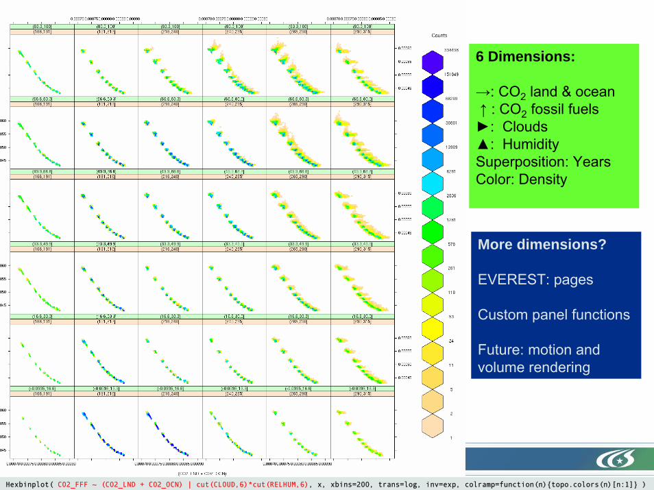
18Hexbinplot( CO2_FFF ~ (CO2_LND + CO2_OCN) | cut(CLOUD,6)*cut(RELHUM,6), x, xbins=200, trans=log, inv=exp, colramp=function(n){topo.colors(n)[n:1]} )

More dimensions?

EVEREST: pages

Custom panel functions

Future: motion and volume rendering

6 Dimensions:

→: CO2 land & ocean↑ : CO2 fossil fuels►: Clouds▲: HumiditySuperposition: YearsColor: Density

19

Running R on the hawk Cluster

Serial R:% module load R

% R

> require(lattice)

>

We are exploring running R in parallel with the snow package:

% srun –N 16 –A

% module load R

> require(snow)

> makeCluster(system(“srunhostname”,TRUE))

>

Starts an R process on each node awaiting snow commands.

Same file system enables reading data and data-parallel processing.

20

The R Project for Statistical Computing www.r-project.org

About RWhat is R?ContributorsScreenshotsWhat's new?

DownloadCRAN

R ProjectFoundationMembers & DonorsMailing ListsBug TrackingDeveloper PageConferencesSearch

DocumentationManualsFAQsNewsletterWikiBooksOther

MiscBioconductorRelated ProjectsLinks

Getting Started:•R is a free software environment for statistical computing and graphics. It compiles and runs on a wide variety of UNIX platforms, Windows and MacOS. To download R, please choose your preferred CRAN mirror. •If you have questions about R like how to download and install the software, or what the license terms are, please read our answers to frequently asked questions before you send an email.

News:•useR! 2007, the first North American useR! will be held at Iowa State University, Ames, Iowa, August 9-10, 2007. •R version 2.4.1 has been released on 2006-12-18. •DSC 2007, the 5th workshop on Directions in Statistical Computing, February 15-16, 2007, Auckland, New Zealand. •R News 6/5 has been published on 2006-12-1. •The R Wiki provides an online forum where useRs can help other useRs.

This server is hosted by the Department of Statistics and Mathematics of the WU Wien.

21

R - Long History and International Support

1976 Bell Labs S-Language: S1, S2, S3, S41988 Insightful Inc. S-Plus1995 R “not unlike S” GPL2002 … R dominates new work in statistics worldwideUsers: number unknown ~100K?

• Excellent graphical tools for exploratory data analysis• The most extensive suite of high dimensional

analysis tools (dimension reduction, clustering, etc.)• Fast prototyping of statistical analysis and empirical

modeling

• Omega project – connectivity: Python, PVM, MPI, SQL, GGobi, NetCDF, HDF

• Parallel: R-ScaLAPACK, Snow, TaskParallel-R

22

Packages are Classified into “Task Views”• Bayesian Inference

• Cluster Analysis

• Econometrics

• Environmetrics

• Empirical Finance

• Statistical Genetics

• Graphics & Visualization

• Machine & Statistical Learning

• Multivariate Statistics

• Statistics for the Social Sciences

• Analysis of Spatial Data

• gRaphical models

~1000 Add-On PackagesRelated Projects• Omega - Distributed Statistical Computing - Connectivity

• Bioconductor – Bioinformatics with R

• R GUIs: Graphical User Interfaces for R

• GGobi – High Dimensional Data Visualization

23

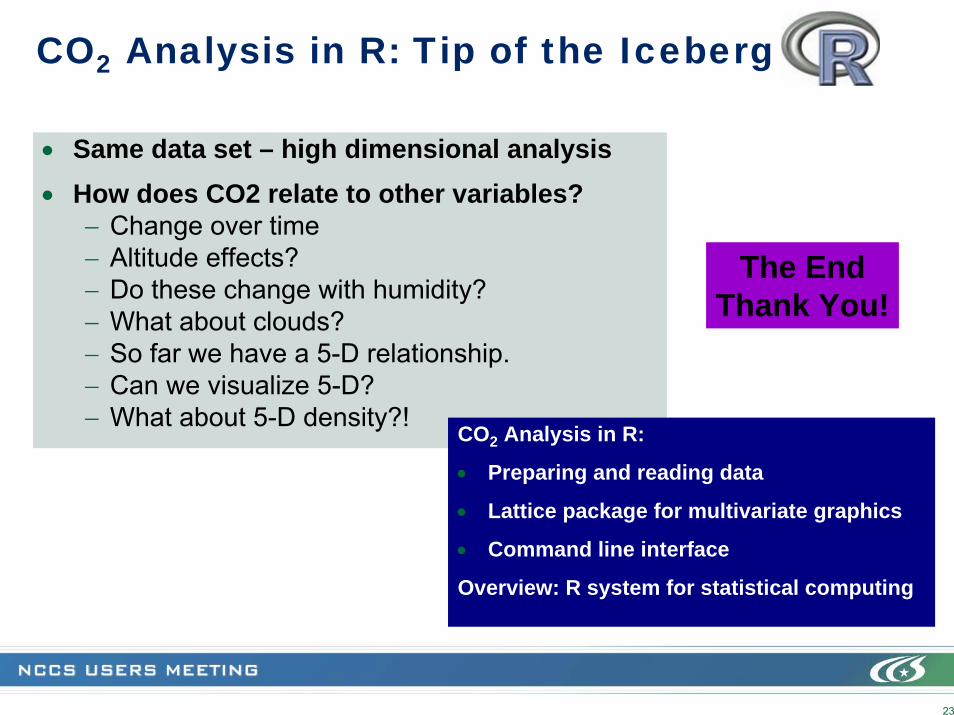
• Same data set – high dimensional analysis• How does CO2 relate to other variables?

− Change over time− Altitude effects?− Do these change with humidity?− What about clouds?− So far we have a 5-D relationship.− Can we visualize 5-D?− What about 5-D density?!

CO2 Analysis in R: Tip of the Iceberg

CO2 Analysis in R:

• Preparing and reading data

• Lattice package for multivariate graphics

• Command line interface

Overview: R system for statistical computing

The EndThank You!