Statistical Considerations in the Study of Obesity€¦ · Overview of Topics • Basic terminology...
105
Statistical Considerations in the Study of Obesity John A. Dawson Post-Doc, Office of Energetics / SSG April 11, 2014
Transcript of Statistical Considerations in the Study of Obesity€¦ · Overview of Topics • Basic terminology...
Statistical Considerations in the Study of Obesity
John A. Dawson
Post-Doc, Office of Energetics / SSG
April 11, 2014
Overview of Topics
• Basic terminology and probability • Randomization • Bias, confounding, blinding and blocking • Simple tests for some very general situations • Am I Normal? What if I’m not? • Fixed vs. random effects • General Considerations as a Statistical Reviewer • Analysis of pre-post experiments • Analysis of cross-over experiments • Analysis of time-to-event data

Basic Terminology and Probability
“Somehow it seems to fill my head with ideas–only I don’t exactly know what they are!”
- Alice, Through the Looking Glass

• Mean • Median • Mode • Quantile • Variance • Standard deviation • *Appending ‘sample’ to the front of any of the above* • Standard error (of the mean) • Coefficient of variation • Precision • Scatterplot • Histogram • Box (and Whisker) plot • Normal (Gaussian) • Standard Normal
Some Basic Terminology
• Null hypothesis (H0) • Alternative hypothesis (HA or H1) • p-value • Type I error • Type II error • Type III error • α (in this context) • β (in this context) • Power • Loss function • Independent variable • Dependent variable • ‘Almost surely’ (a.s.) or ‘with probability 1’ (w.p. 1) • IID
More Basic Terminology
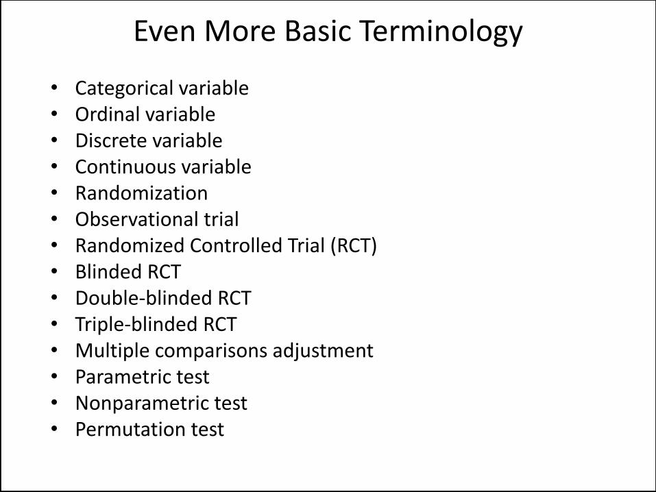
• Categorical variable • Ordinal variable • Discrete variable • Continuous variable • Randomization • Observational trial • Randomized Controlled Trial (RCT) • Blinded RCT • Double-blinded RCT • Triple-blinded RCT • Multiple comparisons adjustment • Parametric test • Nonparametric test • Permutation test
Even More Basic Terminology

• Pr(not A) = 1 – Pr(A) • Pr(A and B) = Pr(A given B)*Pr(B) • Odds (for) event A = Pr(A) / (1 – Pr(A)) • Odds (against) event A = (1 – Pr(A)) / Pr(A) • How many ways are there …
• … to order four items? • … to pick three numbered balls from a bag of six …
• … if order doesn’t matter? • … if order does matter?
• What is Pr(X), where X is …
• … rolling doubles with two dice? • … getting a flush of diamonds from a five-card draw? • … getting any flush from a five-card draw?
Some Simple Probability
Randomization
“To consult a statistician after an experiment is finished is often merely to ask him to conduct a post-mortem examination.”
- R. A. Fisher, Presidential Address to the First Indian Statistical Congress in 1938

• 8 subjects to be randomized to two treatments A and B • One outcome will be measured once for each subject • Q: Is the average outcome the same for A and B?
1 2 3
4 5
6 7 8
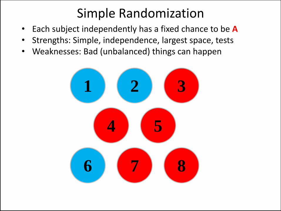
• Each subject independently has a fixed chance to be A • Strengths: Simple, independence, largest space, tests • Weaknesses: Bad (unbalanced) things can happen
1 2 3
4 5
6 7 8
Simple Randomization
1 2 3
4 5
6 7 8
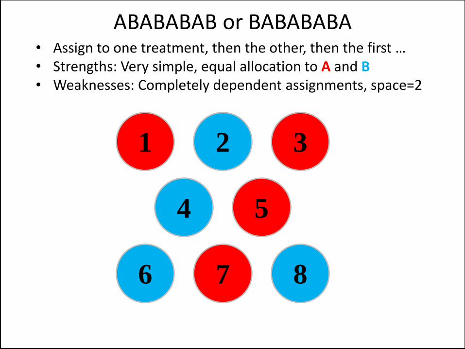
• Assign to one treatment, then the other, then the first … • Strengths: Very simple, equal allocation to A and B • Weaknesses: Completely dependent assignments, space=2
ABABABAB or BABABABA
1 2 3
4 5
6 7 8
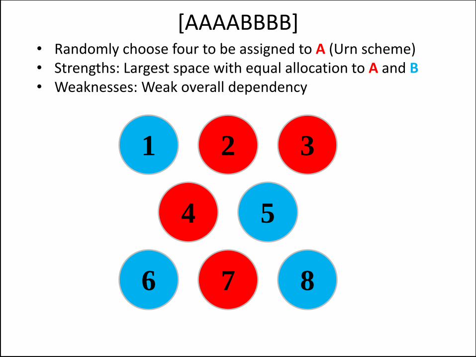
• Randomly choose four to be assigned to A (Urn scheme) • Strengths: Largest space with equal allocation to A and B • Weaknesses: Weak overall dependency
[AAAABBBB]
1 2 3
4 5
6 7 8
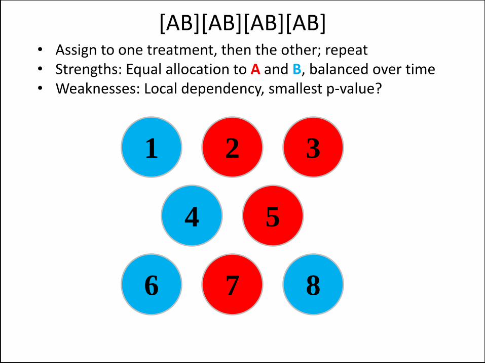
• Assign to one treatment, then the other; repeat • Strengths: Equal allocation to A and B, balanced over time • Weaknesses: Local dependency, smallest p-value?
[AB][AB][AB][AB]
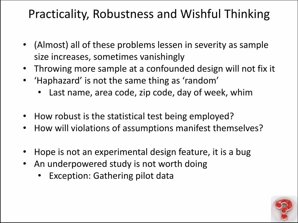
• (Almost) all of these problems lessen in severity as sample size increases, sometimes vanishingly
• Throwing more sample at a confounded design will not fix it • ‘Haphazard’ is not the same thing as ‘random’
• Last name, area code, zip code, day of week, whim
• How robust is the statistical test being employed? • How will violations of assumptions manifest themselves?
• Hope is not an experimental design feature, it is a bug • An underpowered study is not worth doing
• Exception: Gathering pilot data
Practicality, Robustness and Wishful Thinking
Bias, Confounding, Blinding and Blocking
- @HardSciFiMovies, Twitter
When you wish upon a star;
makes no difference who you are;
when you wish upon a star
it biases your actions in favor of the desired outcome.
• Bias has a strictly statistical meaning related to expectations of estimators, but that’s not what we’re focused on here
• Bias: The prior belief for or against something • The efficacy of a treatment compared to SoC • The association between two variables • That eating breakfast promotes weight loss • That sugar is toxic (No! No! Added sugar!)
• Experimental designs ideally should be free of bias from:
• Investigators • Participants / Subjects • Providers of funding
• Solution: Randomize in a blinded manner
Bias
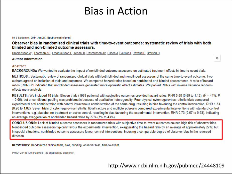
Bias in Action
http://www.ncbi.nlm.nih.gov/pubmed/24448109

• When the effects of two or more covariates cannot be teased apart because of the experimental design, we say they are confounded
• Quite very bad example:
• Confounding is generally avoided through randomization • However, sometimes the groups really need to be balanced
with respect to one or more covariates • Solution: Blocking (not to be confused with stratification)
Confounding
200 Subjects All male
All aged 18 All given Drug A
200 Subjects All female All aged 65
All given Drug B
Group 1 Group 2

• Blind: Being unaware of the treatment assignment • Many levels of blindness as we’ve already touched on
• Blocking: Enforcing balance through local dependencies in
treatment assignment • We’ve seen a few examples of this already • Blockings can correspond to factor levels (day of week) • Blocks need not correspond to a variable at all
• Blocking adds complexity and reduces degrees of freedom • Important: Marginal assignment probabilities are equal
• Sometimes blinding is not completely practical • Blocking can provide opportunities for unblinding
Blinding and Blocking
• Patients: Blind to assignment when possible • Similarly-designed placebos • Sham surgery or brain implants • Deception before debriefing
• Investigators: Blind to assignment when possible • At minimum, blind up until revelation of assignment • Investigators control ‘who comes in the door when’
• Funders: At minimum no role in design implementation
• Options for blinded randomization: • Gather/screen all subjects at once, then randomize • Substitute colors or noninformative labels • Physically implement the randomization (3rd party)
Practical Blinding
• Why block? • Control for day effects • Control for technician effects • Enforce balance over one or many covariates • Account for waves or seasonality
• The last assignment in a block can be determined a.s. • So?
• If single-blinded, clinician knows what’s coming • If blocking structure known, patients can game
system – less of an issue in obesity studies
• One solution is to use randomly determined block sizes • Having others implement a complex randomization protocol
can be fraught with peril
Practical Blocking
• The horrors of clever acronyms
• Sequentially Numbered: By external block or overall • Opaque: So you can’t see inside • Sealed: So that you can’t look inside beforehand • Envelope: Something physical that can be opened with the
subject and can be set up ahead of time
• The numbering / labeling on the outside helps to maintain multiple blocks as well as record keeping
Sequentially Numbered Opaque Sealed Envelope
(SNOSE)
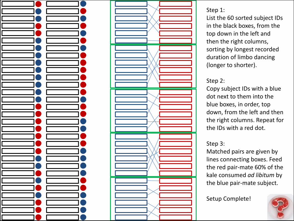
Step 1: List the 60 sorted subject IDs in the black boxes, from the top down in the left and then the right columns, sorting by longest recorded duration of limbo dancing (longer to shorter). Step 2: Copy subject IDs with a blue dot next to them into the blue boxes, in order, top down, from the left and then the right columns. Repeat for the IDs with a red dot. Step 3: Matched pairs are given by lines connecting boxes. Feed the red pair-mate 60% of the kale consumed ad libitum by the blue pair-mate subject. Setup Complete!
Some Simple Tests for Certain General Situations
“Essentially, all models are wrong, some are useful.”
- G.E.P. Box, Empirical Model Building
and Response Surfaces
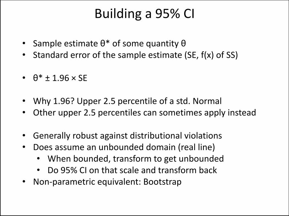
• Sample estimate θ* of some quantity θ • Standard error of the sample estimate (SE, f(x) of SS)
• θ* ± 1.96 × SE
• Why 1.96? Upper 2.5 percentile of a std. Normal • Other upper 2.5 percentiles can sometimes apply instead
• Generally robust against distributional violations • Does assume an unbounded domain (real line)
• When bounded, transform to get unbounded • Do 95% CI on that scale and transform back
• Non-parametric equivalent: Bootstrap
Building a 95% CI
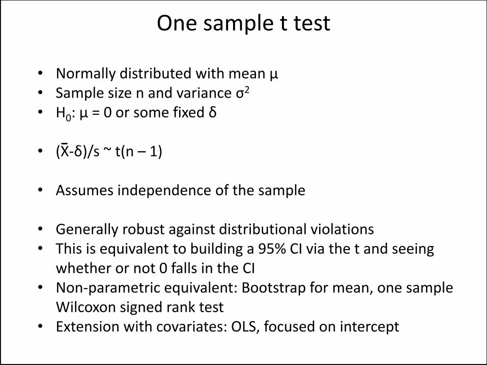
• Normally distributed with mean μ • Sample size n and variance σ2 • H0: μ = 0 or some fixed δ
• (X-δ)/s ~ t(n – 1)
• Assumes independence of the sample
• Generally robust against distributional violations • This is equivalent to building a 95% CI via the t and seeing
whether or not 0 falls in the CI • Non-parametric equivalent: Bootstrap for mean, one sample
Wilcoxon signed rank test • Extension with covariates: OLS, focused on intercept
One sample t test
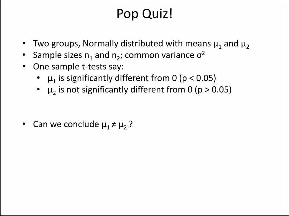
• Two groups, Normally distributed with means μ1 and μ2 • Sample sizes n1 and n2; common variance σ2
• One sample t-tests say: • μ1 is significantly different from 0 (p < 0.05) • μ2 is not significantly different from 0 (p > 0.05)
• Can we conclude μ1 ≠ μ2 ?
Pop Quiz!
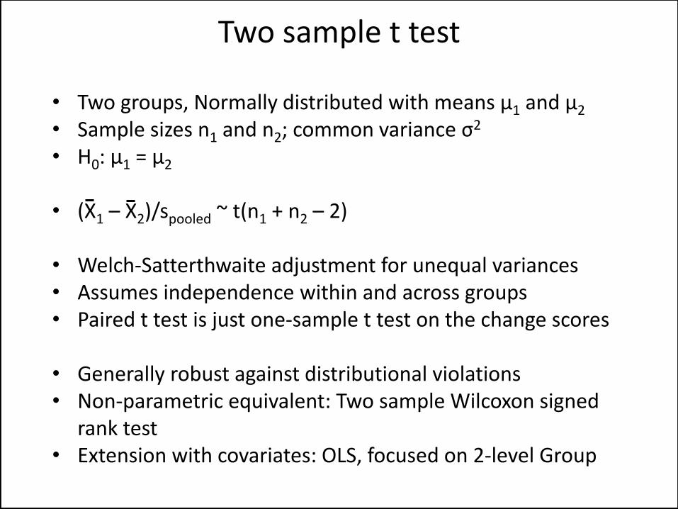
• Two groups, Normally distributed with means μ1 and μ2 • Sample sizes n1 and n2; common variance σ2 • H0: μ1 = μ2
• (X1 – X2)/spooled ~ t(n1 + n2 – 2)
• Welch-Satterthwaite adjustment for unequal variances • Assumes independence within and across groups • Paired t test is just one-sample t test on the change scores
• Generally robust against distributional violations • Non-parametric equivalent: Two sample Wilcoxon signed
rank test • Extension with covariates: OLS, focused on 2-level Group
Two sample t test
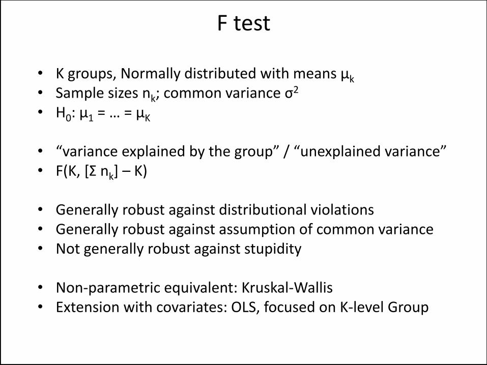
• K groups, Normally distributed with means μk • Sample sizes nk; common variance σ2 • H0: μ1 = … = μK
• “variance explained by the group” / “unexplained variance” • F(K, [Σ nk] – K)
• Generally robust against distributional violations • Generally robust against assumption of common variance • Not generally robust against stupidity
• Non-parametric equivalent: Kruskal-Wallis • Extension with covariates: OLS, focused on K-level Group
F test
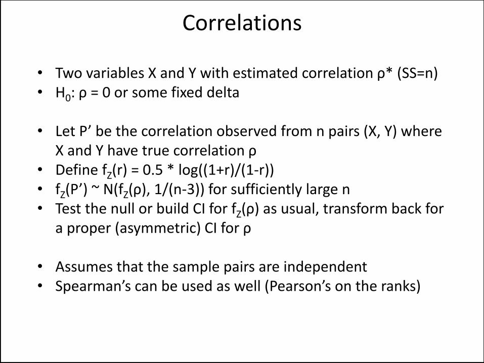
• Two variables X and Y with estimated correlation ρ* (SS=n) • H0: ρ = 0 or some fixed delta
• Let P’ be the correlation observed from n pairs (X, Y) where
X and Y have true correlation ρ • Define fZ(r) = 0.5 * log((1+r)/(1-r)) • fZ(P’) ~ N(fZ(ρ), 1/(n-3)) for sufficiently large n • Test the null or build CI for fZ(ρ) as usual, transform back for
a proper (asymmetric) CI for ρ
• Assumes that the sample pairs are independent • Spearman’s can be used as well (Pearson’s on the ranks)
Correlations
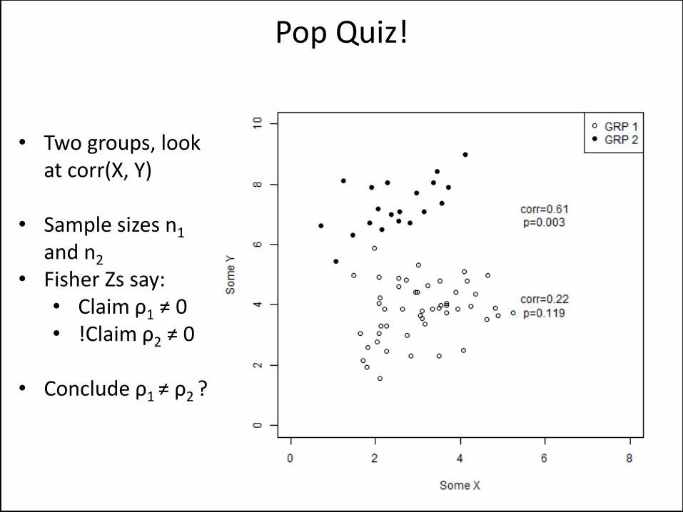
• Two groups, look at corr(X, Y)
• Sample sizes n1 and n2
• Fisher Zs say: • Claim ρ1 ≠ 0 • !Claim ρ2 ≠ 0
• Conclude ρ1 ≠ ρ2 ?
Pop Quiz!
• Series of n trials with yes/no or 1/0 outcomes • What is the probability of success p? • H0: p = some value
• Let X = (# successes). X ~ binom(n, p) • X/n has expectation p, can build CI for p exactly • If you can build a CI, you can do a point equality test • Or: X/n is approximately N(p, p(1-p)/n)
• Use p* in variance; or, p(1-p) bounded above by 0.25 • Approximation not valid for small n
• Assumes that p is fixed • Assumes that the trials are independent
Binomial test of one proportion
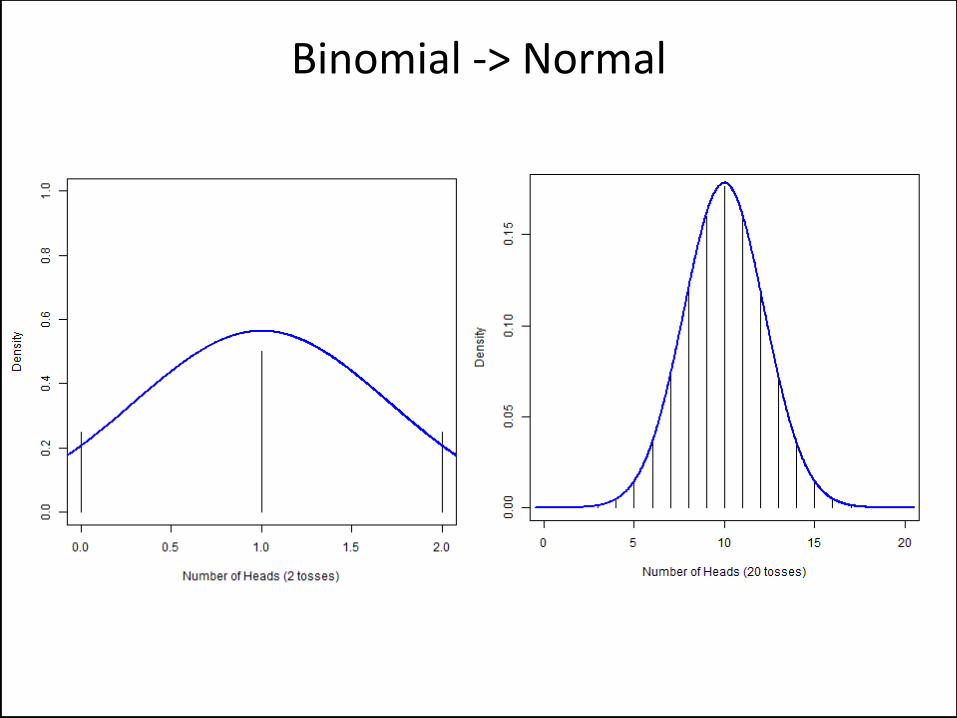
Binomial -> Normal
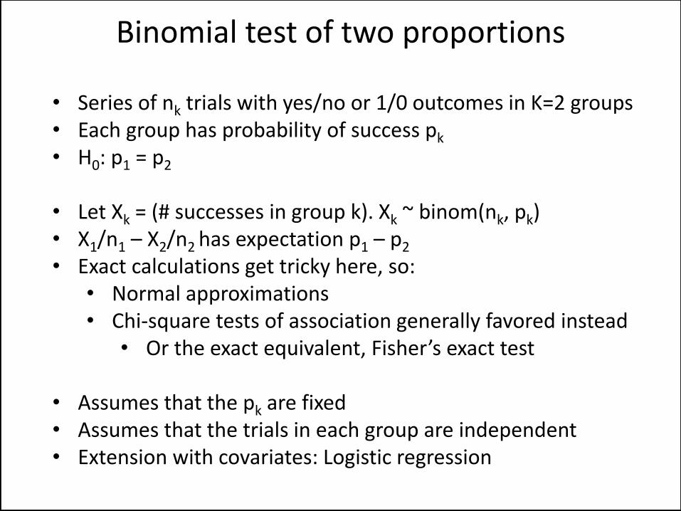
• Series of nk trials with yes/no or 1/0 outcomes in K=2 groups • Each group has probability of success pk
• H0: p1 = p2
• Let Xk = (# successes in group k). Xk ~ binom(nk, pk) • X1/n1 – X2/n2 has expectation p1 – p2 • Exact calculations get tricky here, so:
• Normal approximations • Chi-square tests of association generally favored instead
• Or the exact equivalent, Fisher’s exact test
• Assumes that the pk are fixed • Assumes that the trials in each group are independent • Extension with covariates: Logistic regression
Binomial test of two proportions
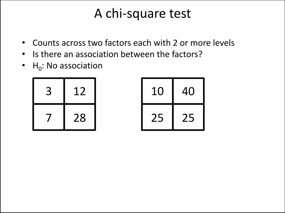
• Counts across two factors each with 2 or more levels • Is there an association between the factors? • H0: No association
A chi-square test
10
25 25
40 3
7 28
12

• Counts across two factors each with 2 or more levels • Is there an association between the factors? • H0: No association
A chi-square test
10
25 25
40 3
7 28
12
10 40
35
15
35 65
50
50
50 100
17.5 10 ∗ 15
50= 3
10 ∗ 35
50= 7
40 ∗ 15
50= 12
40 ∗ 35
50= 28
32.5
17.5 32.5
E
O

• Counts across two factors each with 2 or more levels • Is there an association between the factors? • H0: No association
A chi-square test
3
7 28
12
10 40
35
15
50
10 ∗ 15
50= 3
10 ∗ 35
50= 7
40 ∗ 15
50= 12
40 ∗ 35
50= 28
E
O
(𝑂−𝐸)2
𝐸 = 0 + 0 + 0 + 0
= 0 on (2-1)*(2-1) = 1 d.f. (p = 1)
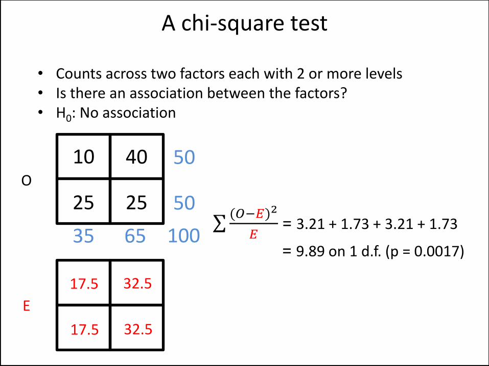
• Counts across two factors each with 2 or more levels • Is there an association between the factors? • H0: No association
A chi-square test
10
25 25
40
35 65
50
50
100
17.5 32.5
17.5 32.5
E
O
(𝑂−𝐸)2
𝐸 = 3.21 + 1.73 + 3.21 + 1.73
= 9.89 on 1 d.f. (p = 0.0017)
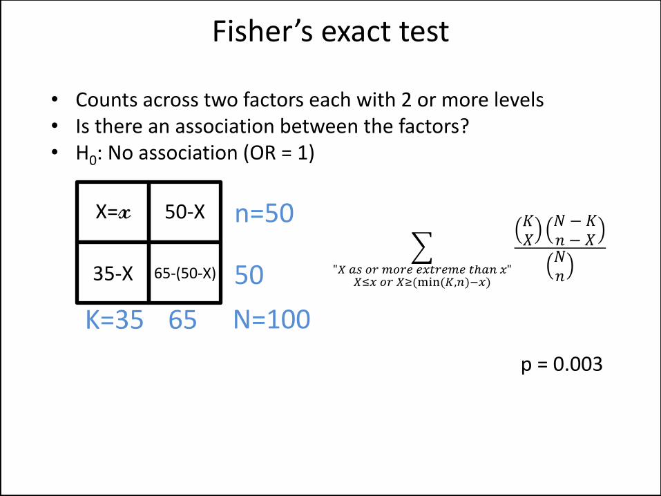
Fisher’s exact test
• Counts across two factors each with 2 or more levels • Is there an association between the factors? • H0: No association (OR = 1)
X=x
35-X 65-(50-X)
50-X
K=35 65
50
n=50
N=100
p = 0.003
𝐾𝑋𝑁 − 𝐾𝑛 − 𝑋𝑁𝑛"𝑋 𝑎𝑠 𝑜𝑟 𝑚𝑜𝑟𝑒 𝑒𝑥𝑡𝑟𝑒𝑚𝑒 𝑡ℎ𝑎𝑛 𝑥"
𝑋≤𝑥 𝑜𝑟 𝑋≥(min (𝐾,𝑛)−𝑥)
• Counts across two factors each with 2 or more levels • Is there an association between the factors? • H0: No association
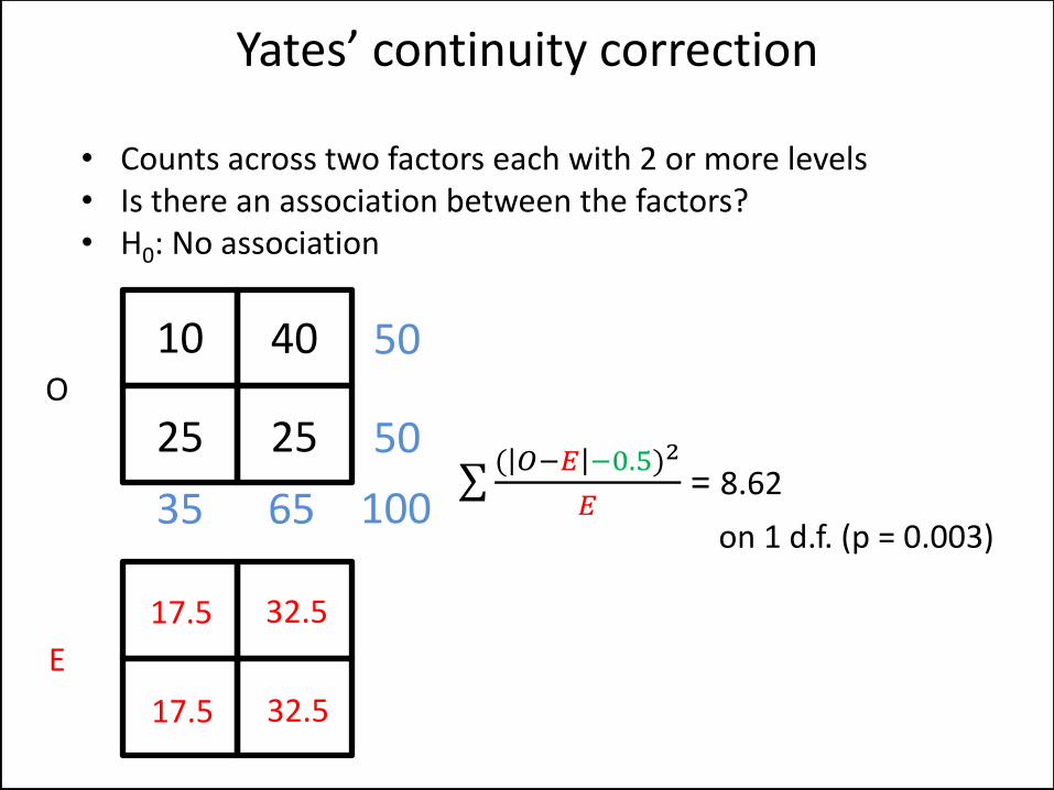
Yates’ continuity correction
10
25 25
40
35 65
50
50
100
17.5 32.5
17.5 32.5
E
O
( 𝑂−𝐸 −0.5)2
𝐸 = 8.62
on 1 d.f. (p = 0.003)

• Continuous outcome Y • Predictors / covariates: X1, X2, …, Xm • Sample size n, indexed by j • “Y is a linear function of the predictors” • Yj = α0 + β1*X1j + … + βm*Xmj + εj
• Which βs are different from 0? • εj ~ i.i.d. N(0, σ2)
• Generally robust against distributional violations • Generally robust against assumption of equal variance
across various values of α0 + Xβ • Non-parametric equivalent: Permutation test overlay • We’ll have lots more on this in the next section
Linear regression
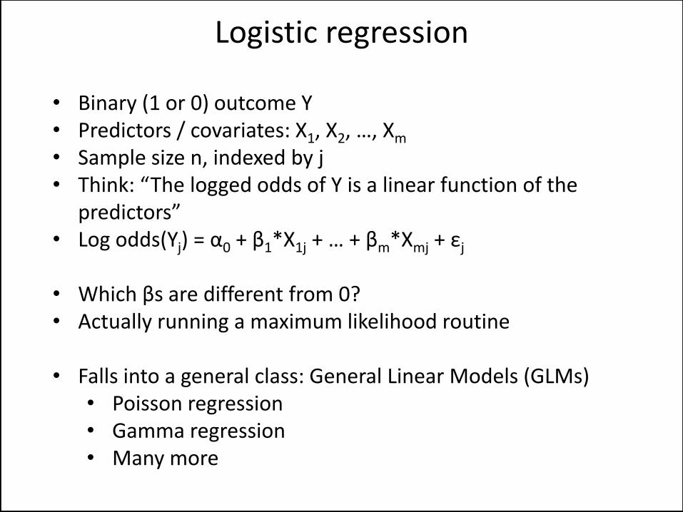
• Binary (1 or 0) outcome Y • Predictors / covariates: X1, X2, …, Xm • Sample size n, indexed by j • Think: “The logged odds of Y is a linear function of the
predictors” • Log odds(Yj) = α0 + β1*X1j + … + βm*Xmj + εj
• Which βs are different from 0? • Actually running a maximum likelihood routine
• Falls into a general class: General Linear Models (GLMs)
• Poisson regression • Gamma regression • Many more
Logistic regression

• From The Guardian on March 5, 2014: • “So the people we think of as protein-loons were always
eating other stuff beside [sic] it. They are still going to live longer than you. In a longitudinal population study I've been doing, I have demonstrated that just knowing how to pronounce ‘quinoa’ extends your life expectancy by 12 years.”
• Has your life expectancy just been extended by 12 years?
Pop Quiz!
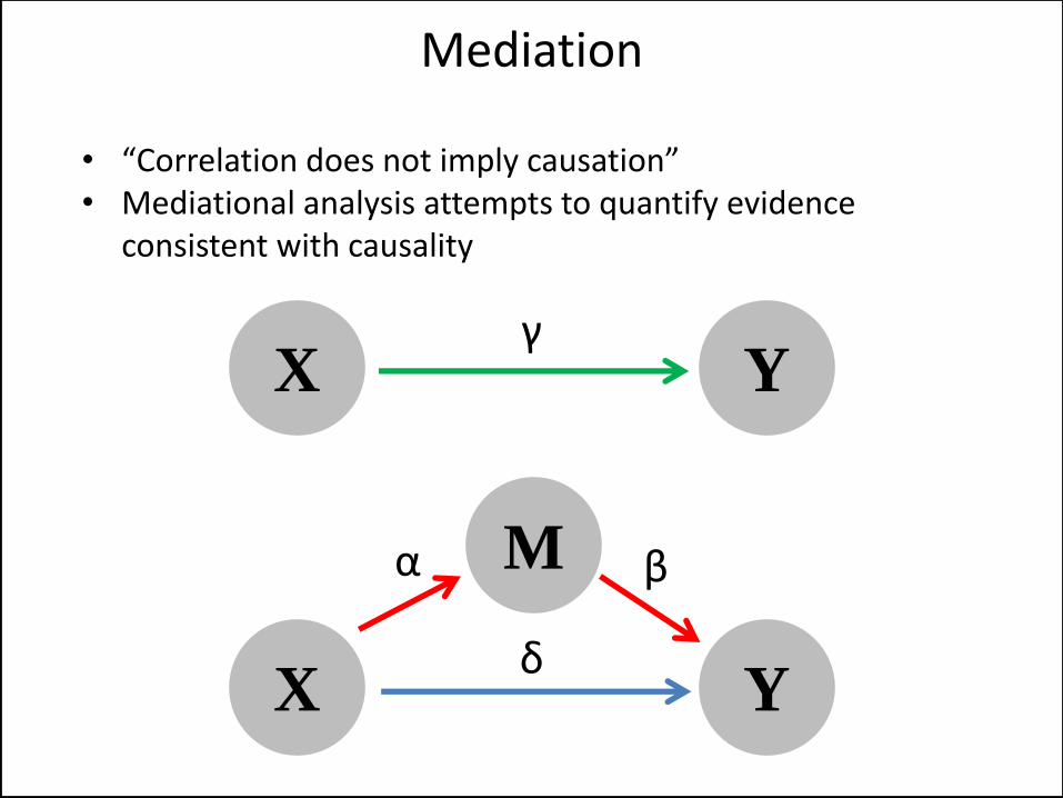
• “Correlation does not imply causation” • Mediational analysis attempts to quantify evidence
consistent with causality
Mediation
M
X Y
X Y γ
α β
δ

• The SE for αβ is not Normal, so bootstrap for it • Mediational analysis is made under the assumption of a
causal mediator (and only the given mediator(s)) ! • Thus it should really not be used as a test for causality
• Can be useful for probabilistically ruling out potential
mediators
Mediation: Caveats
M
X Y
α β
δ
• We’ll cover the following in greater detail later:
• Pre-post designs (OLS, MEMs or GLMs)
• Cross-over designs (OLS, MEMs or GLMs)
• Time-to-event outcomes (censored outcomes)
Some other situations
Am I Normal? What If I’m Not?
“Standard Deviation Not Enough For Perverted Statistician.”
- Fake teaser, The Onion
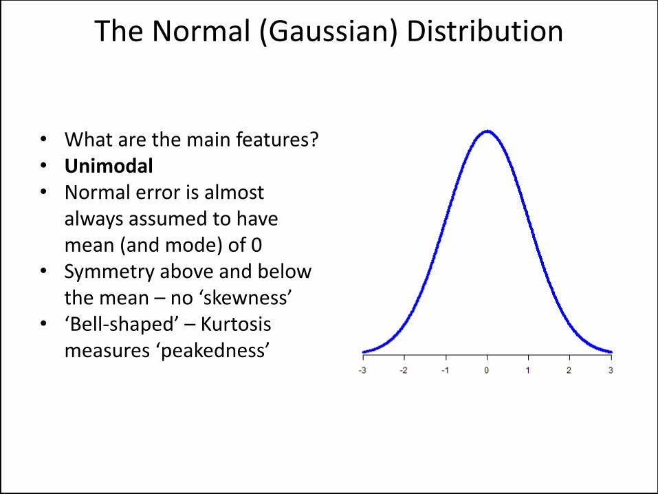
• What are the main features? • Unimodal • Normal error is almost
always assumed to have mean (and mode) of 0
• Symmetry above and below the mean – no ‘skewness’
• ‘Bell-shaped’ – Kurtosis measures ‘peakedness’
The Normal (Gaussian) Distribution
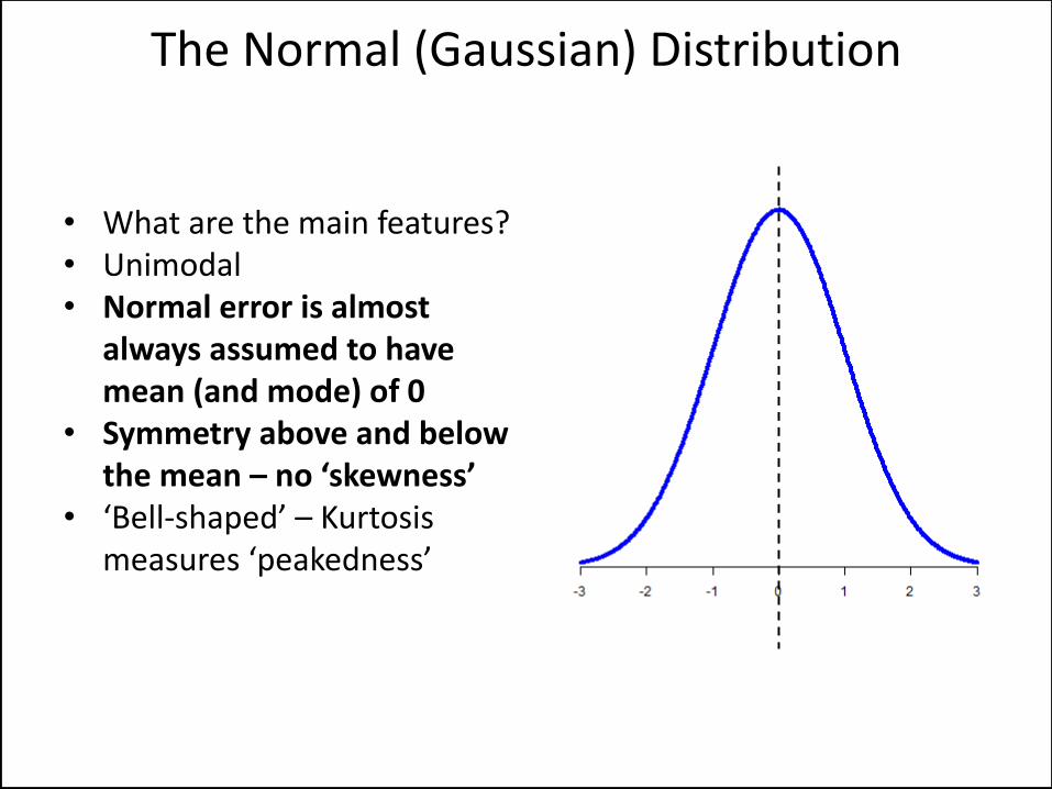
• What are the main features? • Unimodal • Normal error is almost
always assumed to have mean (and mode) of 0
• Symmetry above and below the mean – no ‘skewness’
• ‘Bell-shaped’ – Kurtosis measures ‘peakedness’
The Normal (Gaussian) Distribution
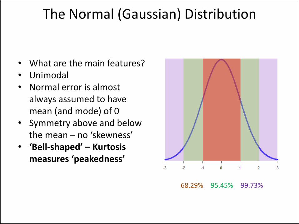
• What are the main features? • Unimodal • Normal error is almost
always assumed to have mean (and mode) of 0
• Symmetry above and below the mean – no ‘skewness’
• ‘Bell-shaped’ – Kurtosis measures ‘peakedness’
The Normal (Gaussian) Distribution
68.29% 95.45% 99.73%
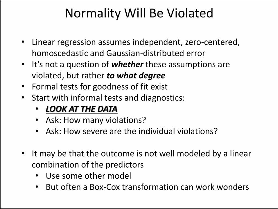
• Linear regression assumes independent, zero-centered, homoscedastic and Gaussian-distributed error
• It’s not a question of whether these assumptions are violated, but rather to what degree
• Formal tests for goodness of fit exist • Start with informal tests and diagnostics:
• LOOK AT THE DATA • Ask: How many violations? • Ask: How severe are the individual violations?
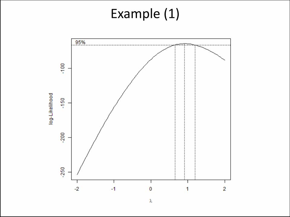
• It may be that the outcome is not well modeled by a linear
combination of the predictors • Use some other model • But often a Box-Cox transformation can work wonders
Normality Will Be Violated

Example (1)
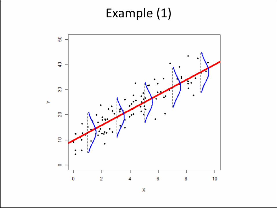
Example (1)
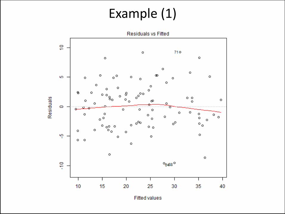
Example (1)
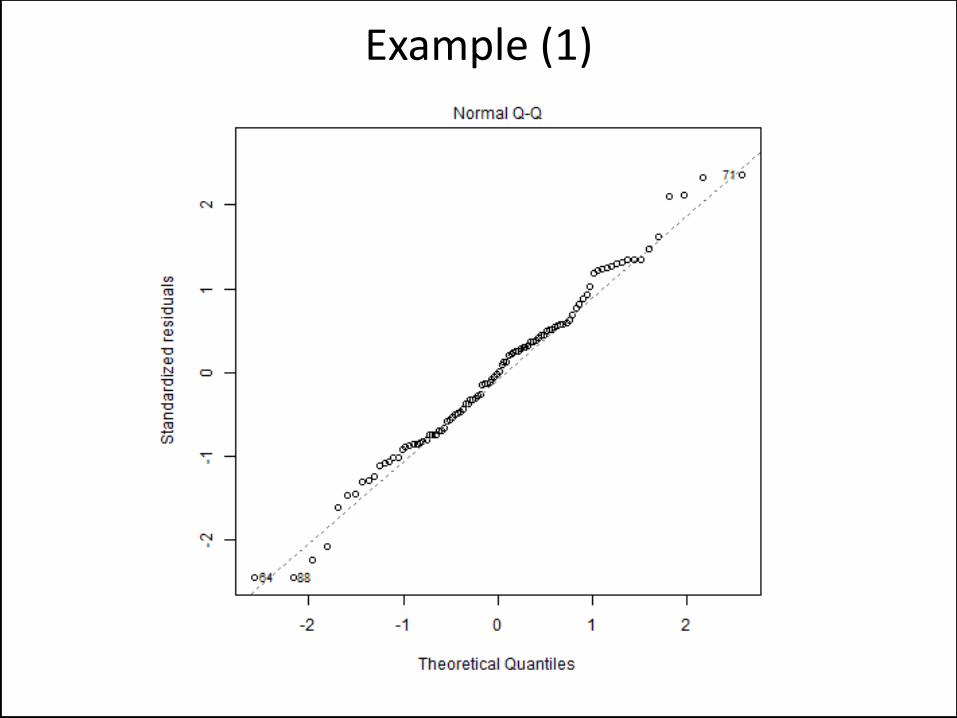
Example (1)
Example (1)
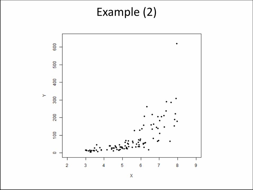
Example (2)

Example (2)

Example (2)
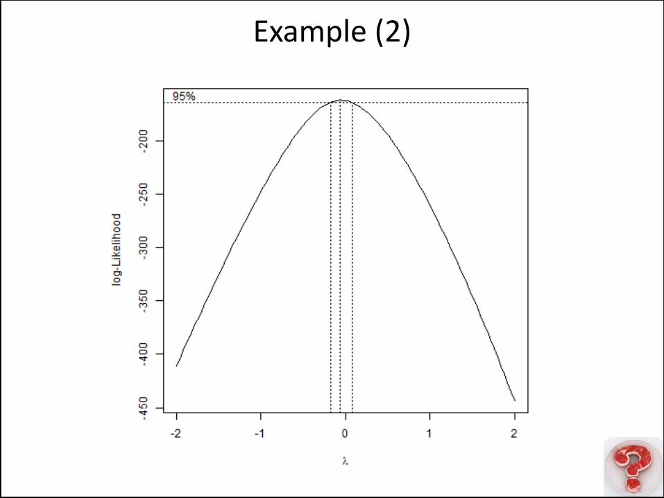
Example (2)

Fixed vs. Random Effects
“Measure twice, cut once.”
- Unknown
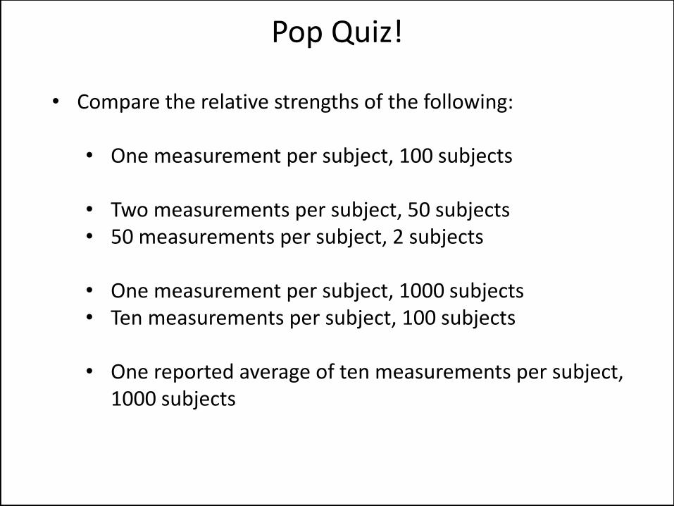
• Compare the relative strengths of the following: • One measurement per subject, 100 subjects
• Two measurements per subject, 50 subjects • 50 measurements per subject, 2 subjects
• One measurement per subject, 1000 subjects • Ten measurements per subject, 100 subjects
• One reported average of ten measurements per subject,
1000 subjects
Pop Quiz!
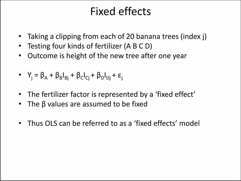
• Taking a clipping from each of 20 banana trees (index j) • Testing four kinds of fertilizer (A B C D) • Outcome is height of the new tree after one year
• Yj = βA + βBIBj + βCICj + βDIDj + εj
• The fertilizer factor is represented by a ‘fixed effect’ • The β values are assumed to be fixed
• Thus OLS can be referred to as a ‘fixed effects’ model
Fixed effects
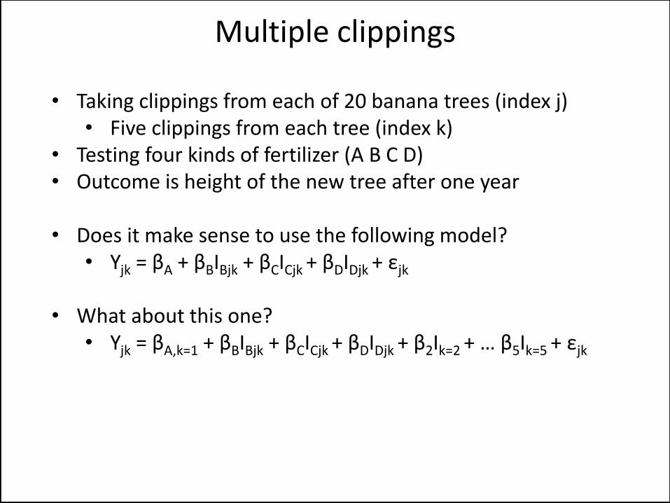
• Taking clippings from each of 20 banana trees (index j) • Five clippings from each tree (index k)
• Testing four kinds of fertilizer (A B C D) • Outcome is height of the new tree after one year
• Does it make sense to use the following model?
• Yjk = βA + βBIBjk + βCICjk + βDIDjk + εjk
• What about this one?
• Yjk = βA,k=1 + βBIBjk + βCICjk + βDIDjk + β2Ik=2 + … β5Ik=5 + εjk
Multiple clippings
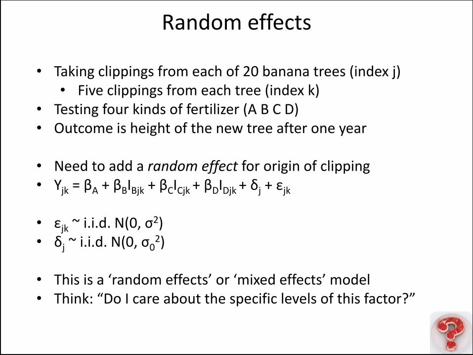
• Taking clippings from each of 20 banana trees (index j) • Five clippings from each tree (index k)
• Testing four kinds of fertilizer (A B C D) • Outcome is height of the new tree after one year
• Need to add a random effect for origin of clipping • Yjk = βA + βBIBjk + βCICjk + βDIDjk + δj + εjk
• εjk ~ i.i.d. N(0, σ2) • δj ~ i.i.d. N(0, σ0
2)
• This is a ‘random effects’ or ‘mixed effects’ model • Think: “Do I care about the specific levels of this factor?”
Random effects
General Considerations as a Statistical Reviewer
“Lies, damned lies, and statistics.”
- Attributed to Benjamin Disraeli, popularized by Mark Twain, Chapters from My Autobiography
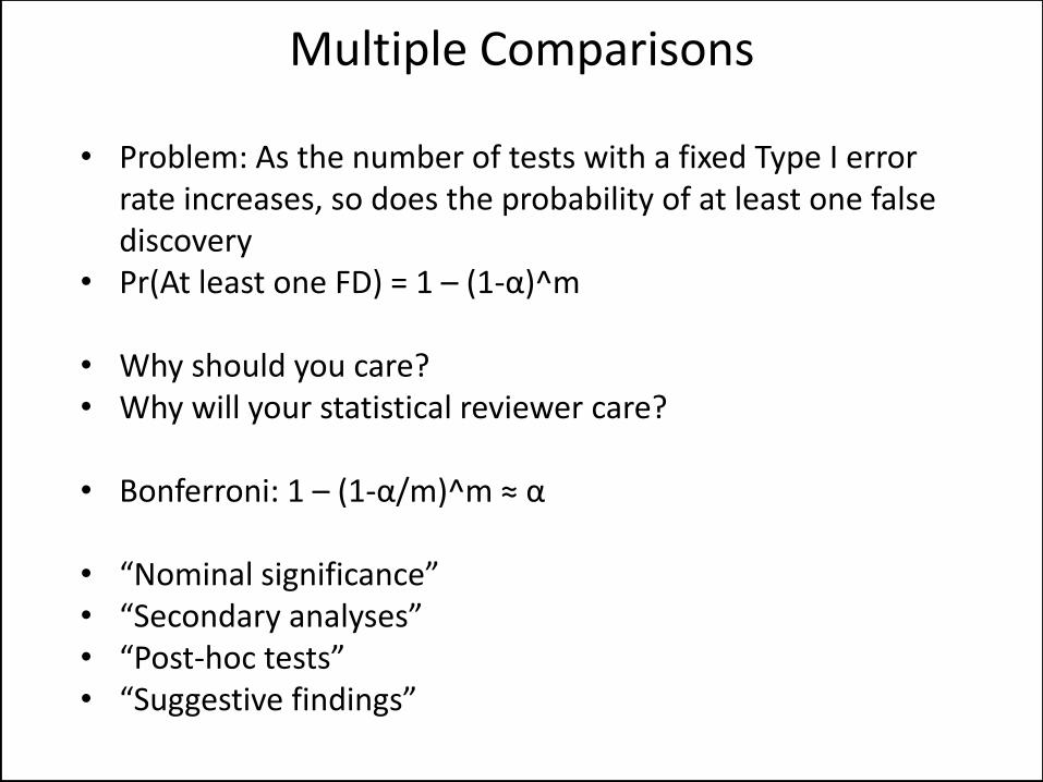
• Problem: As the number of tests with a fixed Type I error rate increases, so does the probability of at least one false discovery
• Pr(At least one FD) = 1 – (1-α)^m
• Why should you care? • Why will your statistical reviewer care?
• Bonferroni: 1 – (1-α/m)^m ≈ α
• “Nominal significance” • “Secondary analyses” • “Post-hoc tests” • “Suggestive findings”
Multiple Comparisons
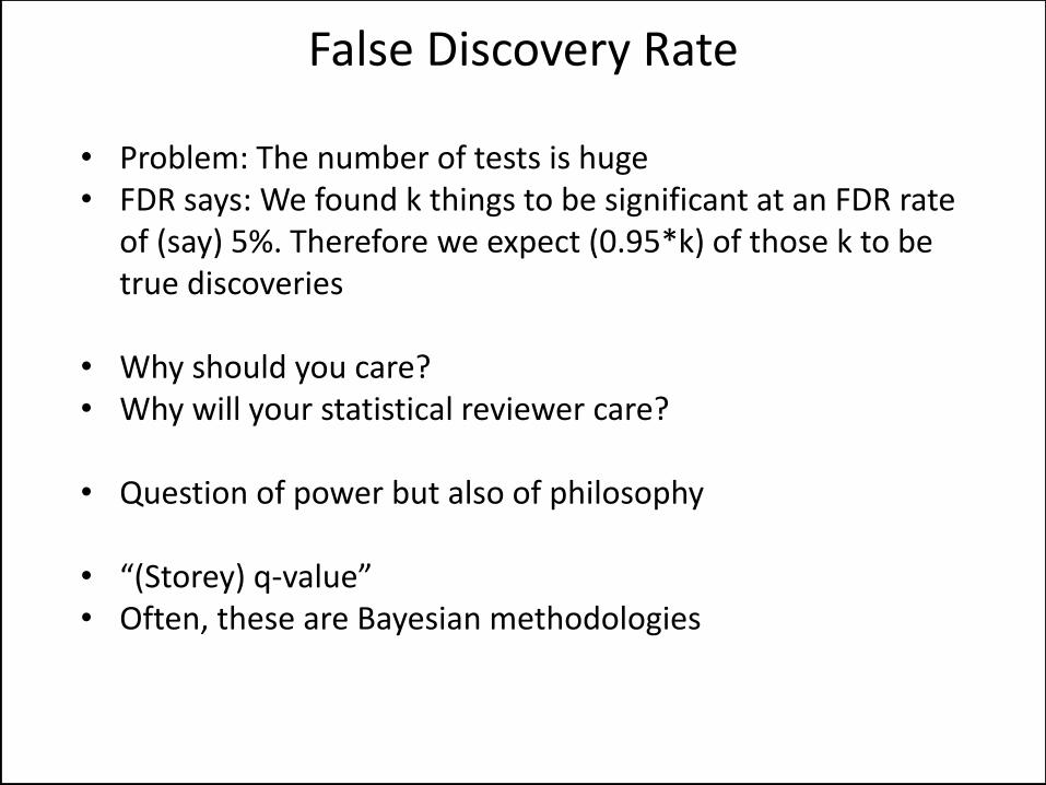
• Problem: The number of tests is huge • FDR says: We found k things to be significant at an FDR rate
of (say) 5%. Therefore we expect (0.95*k) of those k to be true discoveries
• Why should you care? • Why will your statistical reviewer care?
• Question of power but also of philosophy
• “(Storey) q-value” • Often, these are Bayesian methodologies
False Discovery Rate
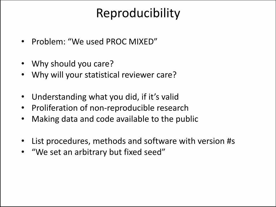
• Problem: “We used PROC MIXED”
• Why should you care? • Why will your statistical reviewer care?
• Understanding what you did, if it’s valid • Proliferation of non-reproducible research • Making data and code available to the public
• List procedures, methods and software with version #s • “We set an arbitrary but fixed seed”
Reproducibility
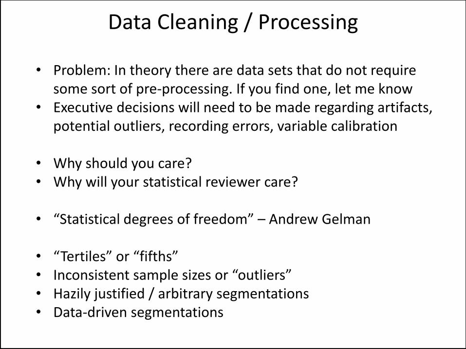
• Problem: In theory there are data sets that do not require some sort of pre-processing. If you find one, let me know
• Executive decisions will need to be made regarding artifacts, potential outliers, recording errors, variable calibration
• Why should you care? • Why will your statistical reviewer care?
• “Statistical degrees of freedom” – Andrew Gelman
• “Tertiles” or “fifths” • Inconsistent sample sizes or “outliers” • Hazily justified / arbitrary segmentations • Data-driven segmentations
Data Cleaning / Processing
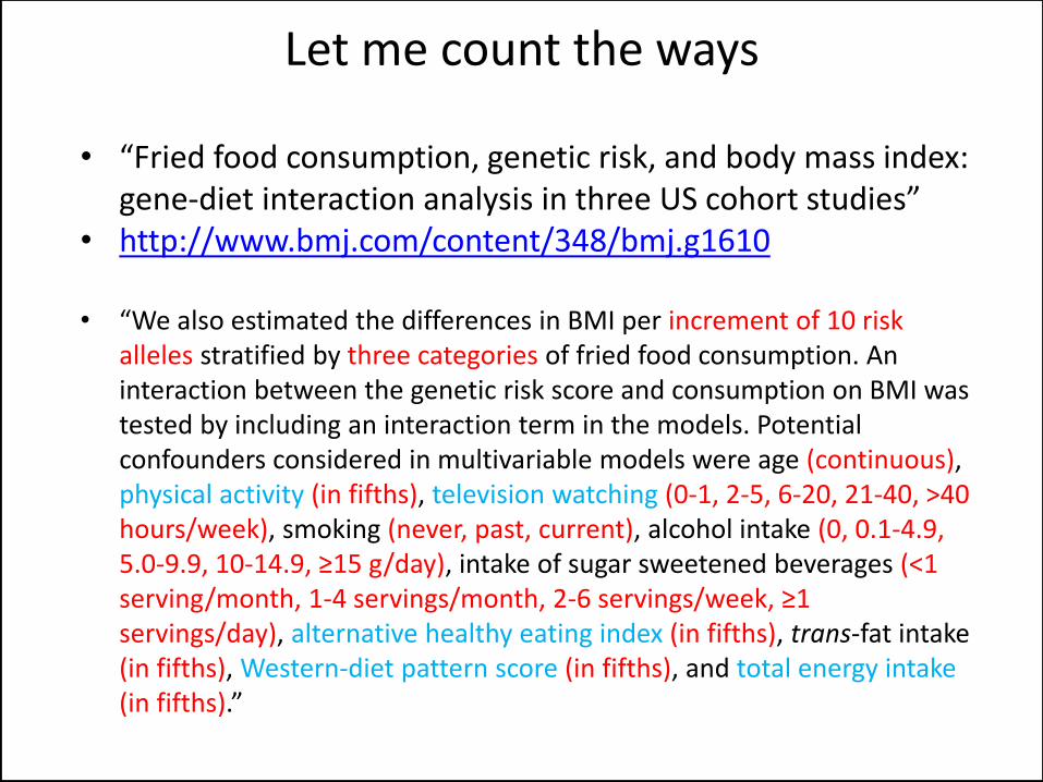
• “Fried food consumption, genetic risk, and body mass index: gene-diet interaction analysis in three US cohort studies”
• http://www.bmj.com/content/348/bmj.g1610
• “We also estimated the differences in BMI per increment of 10 risk alleles stratified by three categories of fried food consumption. An interaction between the genetic risk score and consumption on BMI was tested by including an interaction term in the models. Potential confounders considered in multivariable models were age (continuous), physical activity (in fifths), television watching (0-1, 2-5, 6-20, 21-40, >40 hours/week), smoking (never, past, current), alcohol intake (0, 0.1-4.9, 5.0-9.9, 10-14.9, ≥15 g/day), intake of sugar sweetened beverages (<1 serving/month, 1-4 servings/month, 2-6 servings/week, ≥1 servings/day), alternative healthy eating index (in fifths), trans-fat intake (in fifths), Western-diet pattern score (in fifths), and total energy intake (in fifths).”
Let me count the ways
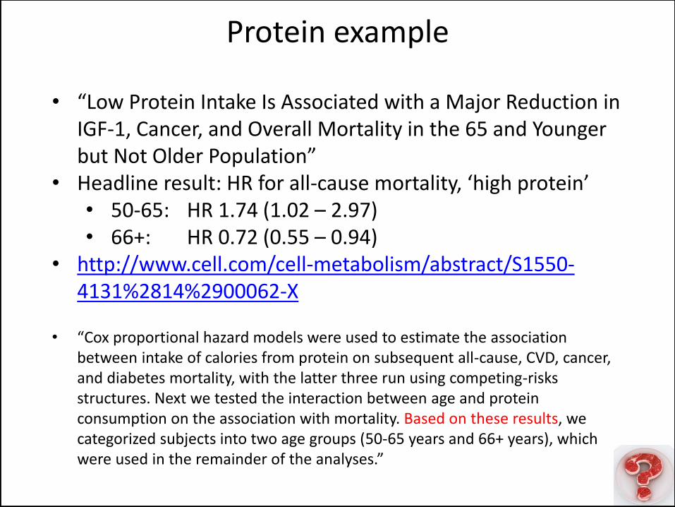
• “Low Protein Intake Is Associated with a Major Reduction in IGF-1, Cancer, and Overall Mortality in the 65 and Younger but Not Older Population”
• Headline result: HR for all-cause mortality, ‘high protein’ • 50-65: HR 1.74 (1.02 – 2.97) • 66+: HR 0.72 (0.55 – 0.94)
• http://www.cell.com/cell-metabolism/abstract/S1550-4131%2814%2900062-X
• “Cox proportional hazard models were used to estimate the association
between intake of calories from protein on subsequent all-cause, CVD, cancer, and diabetes mortality, with the latter three run using competing-risks structures. Next we tested the interaction between age and protein consumption on the association with mortality. Based on these results, we categorized subjects into two age groups (50-65 years and 66+ years), which were used in the remainder of the analyses.”
Protein example
Analysis of Pre-Post Experiments
“I’m not the same man I was yesterday, am I?”
- Sanzo, Saiyuki
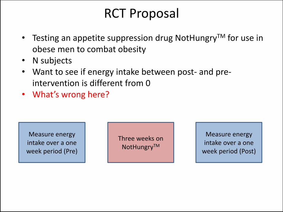
• Testing an appetite suppression drug NotHungryTM for use in obese men to combat obesity
• N subjects • Want to see if energy intake between post- and pre-
intervention is different from 0 • What’s wrong here?
RCT Proposal
Measure energy intake over a one week period (Pre)
Measure energy intake over a one
week period (Post)
Three weeks on NotHungryTM
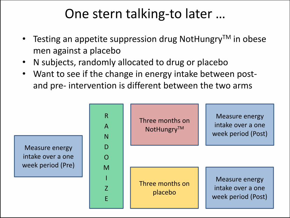
• Testing an appetite suppression drug NotHungryTM in obese men against a placebo
• N subjects, randomly allocated to drug or placebo • Want to see if the change in energy intake between post-
and pre- intervention is different between the two arms
One stern talking-to later …
Measure energy intake over a one
week period (Post)
Three months on NotHungryTM
Measure energy intake over a one
week period (Post)
Three months on placebo
R
A
N
D
O
M
I
Z
E
Measure energy intake over a one week period (Pre)
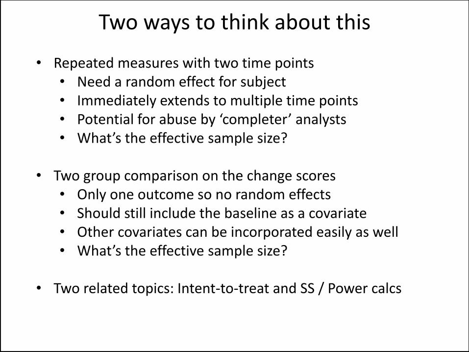
• Repeated measures with two time points • Need a random effect for subject • Immediately extends to multiple time points • Potential for abuse by ‘completer’ analysts • What’s the effective sample size?
• Two group comparison on the change scores
• Only one outcome so no random effects • Should still include the baseline as a covariate • Other covariates can be incorporated easily as well • What’s the effective sample size?
• Two related topics: Intent-to-treat and SS / Power calcs
Two ways to think about this

• Related issue not specific to pre-post designs • Generally subjects are coded according to the group to
which they were randomized • This is called an intent-to-treat analysis
• Subjects may not be in compliance
• Stop taking the drug because of side effects • Off-label use of a medication
• Taking this into account is an as-treated analysis
• What are the relative merits? • How do these change interpretation? • What do governmental regulatory agencies say?
Intent-to-treat
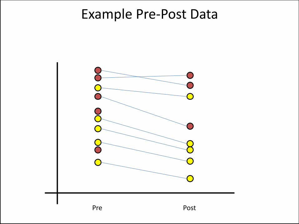
Example Pre-Post Data
Pre Post
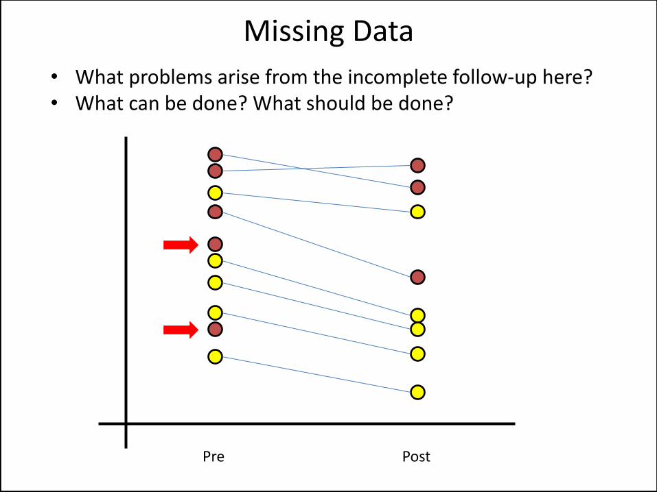
• What problems arise from the incomplete follow-up here? • What can be done? What should be done?
Missing Data
Pre Post
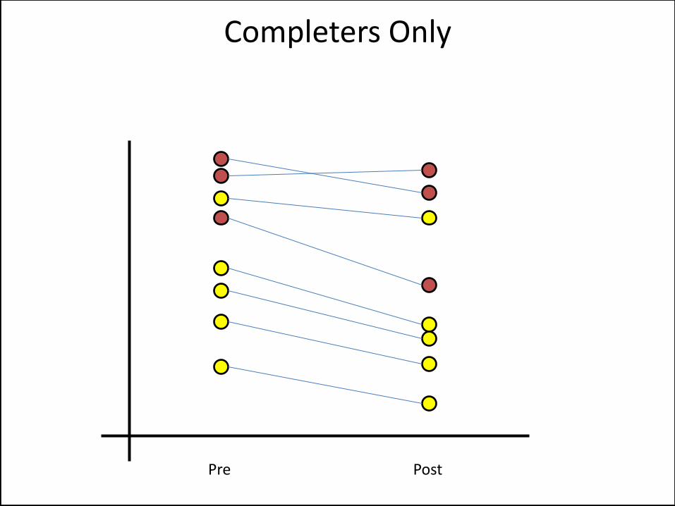
Completers Only
Pre Post

LOCF
Pre Post
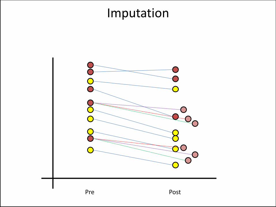
Imputation
Pre Post
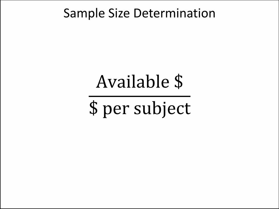
Sample Size Determination
Available $
$ per subject
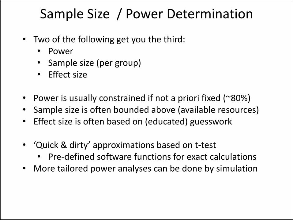
• Two of the following get you the third: • Power • Sample size (per group) • Effect size
• Power is usually constrained if not a priori fixed (~80%) • Sample size is often bounded above (available resources) • Effect size is often based on (educated) guesswork
• ‘Quick & dirty’ approximations based on t-test
• Pre-defined software functions for exact calculations • More tailored power analyses can be done by simulation
Sample Size / Power Determination

• ‘Signal-to-noise’ ratio • | μ1 – μ2 | / σ • Unitless • In this example the
true effect size is 4
• Estimated with sample plug-ins
• Cohen’s d uses the equal-variance t-test estimate of the pooled variance
• Hedge’s g uses the estimate from Welch’s t-test
What’s the Effect Size?

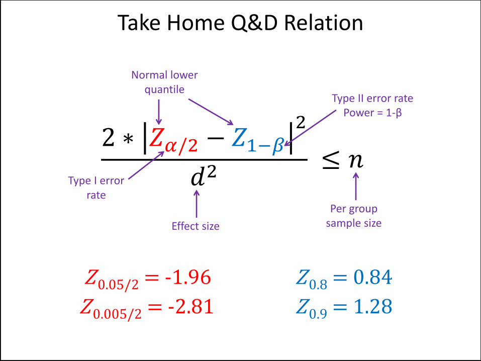
Take Home Q&D Relation
2 ∗ 𝑍𝛼/2 − 𝑍1−𝛽2
𝑑2 ≤ 𝑛
Take Home Q&D Relation
2 ∗ 𝑍𝛼/2 − 𝑍1−𝛽2
𝑑2 ≤ 𝑛
Effect size
Type I error rate
Type II error rate Power = 1-β
Per group sample size
Normal lower quantile
Z 0.05/2 = -1.96
Z 0.005/2 = -2.81
Z 0.8 = 0.84
Z 0.9 = 1.28
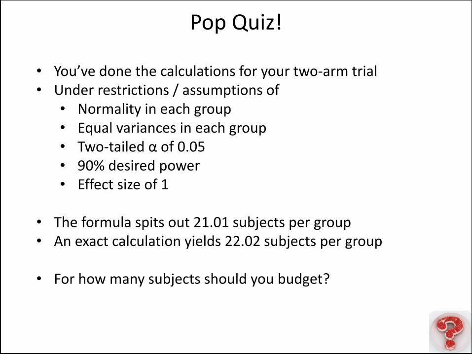
• You’ve done the calculations for your two-arm trial • Under restrictions / assumptions of
• Normality in each group • Equal variances in each group • Two-tailed α of 0.05 • 90% desired power • Effect size of 1
• The formula spits out 21.01 subjects per group • An exact calculation yields 22.02 subjects per group
• For how many subjects should you budget?
Pop Quiz!

Analysis of Cross-over Experiments
“I owe my solitude to other people.”
- Attributed to Alan Watts
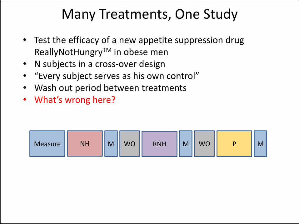
• Test the efficacy of a new appetite suppression drug ReallyNotHungryTM in obese men
• N subjects in a cross-over design • “Every subject serves as his own control” • Wash out period between treatments • What’s wrong here?
Many Treatments, One Study
Measure NH M RNH P WO M WO M
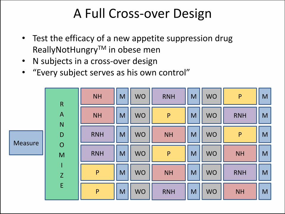
• Test the efficacy of a new appetite suppression drug ReallyNotHungryTM in obese men
• N subjects in a cross-over design • “Every subject serves as his own control”
A Full Cross-over Design
Measure
NH M RNH P WO M WO M R
A
N
D
O
M
I
Z
E
NH M P RNH WO M WO M
RNH M NH P WO M WO M
RNH M P NH WO M WO M
P M NH RNH WO M WO M
P M RNH NH WO M WO M
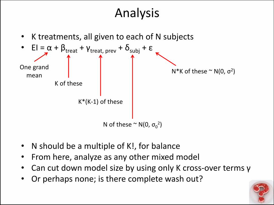
• K treatments, all given to each of N subjects • EI = α + βtreat + γtreat, prev + δsubj + ε
• N should be a multiple of K!, for balance • From here, analyze as any other mixed model • Can cut down model size by using only K cross-over terms γ • Or perhaps none; is there complete wash out?
Analysis
K of these
K*(K-1) of these
N of these ~ N(0, σ02)
N*K of these ~ N(0, σ2) One grand
mean
Analysis of Time-to-event data
“Ask her to wait a moment – I am almost done.”
- C. F. Gauss, as recorded in Men of Mathematics

Why are time-to-event data special?
• Given the data below, how might we analyze them? • t-test • Count models (Poisson, negative binomial)
• What if there are missing data?
• We can impute much of this problem away
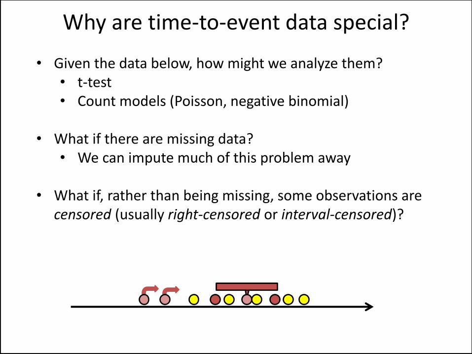
Why are time-to-event data special?
• Given the data below, how might we analyze them? • t-test • Count models (Poisson, negative binomial)
• What if there are missing data?
• We can impute much of this problem away
• What if, rather than being missing, some observations are censored (usually right-censored or interval-censored)?
Why are time-to-event data special?
• Examples of time-to-event data: • Time to death (Survival) • Time to recurrence • Time to first myocardial infarction • Time to first alcoholic drink • Time to first marriage • … total reproduction? • … number of food pellets eaten?
• Partial information • Need to incorporate that information into the analysis
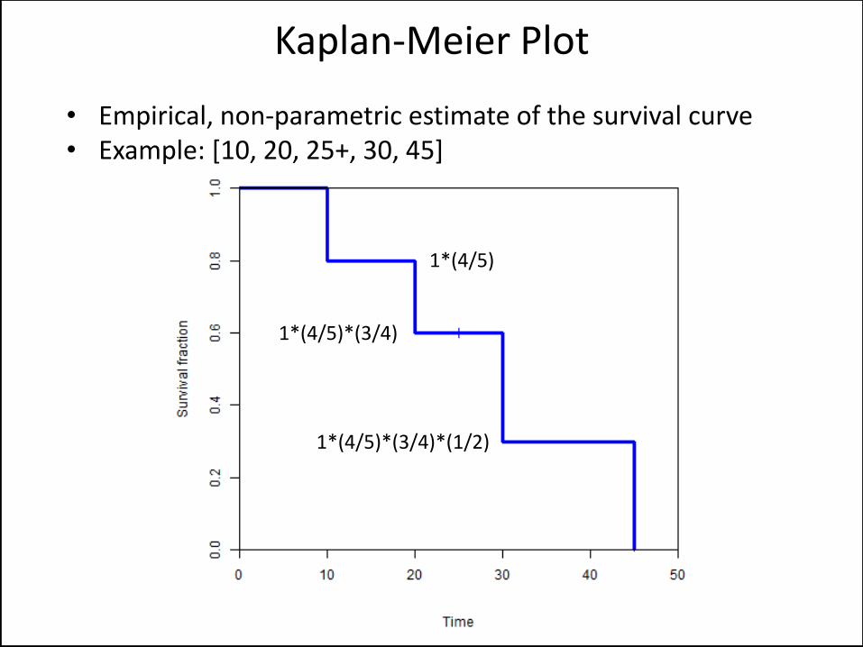
• Empirical, non-parametric estimate of the survival curve • Example: [10, 20, 25+, 30, 45]
Kaplan-Meier Plot
1*(4/5)
1*(4/5)*(3/4)
1*(4/5)*(3/4)*(1/2)
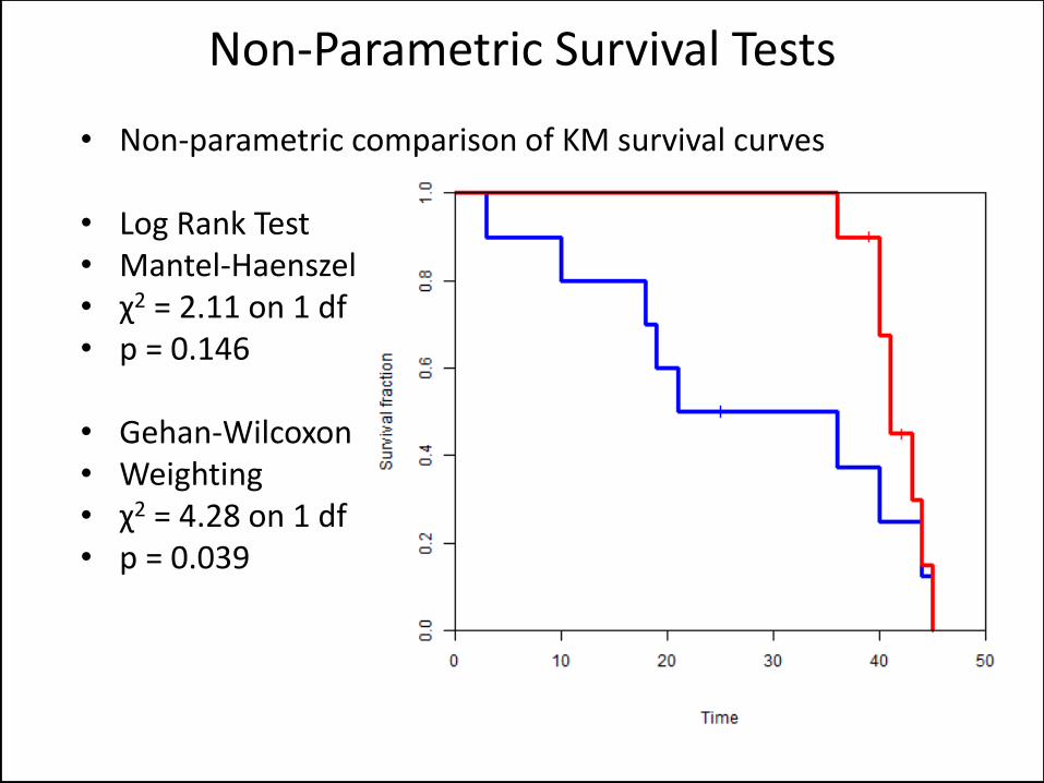
• Non-parametric comparison of KM survival curves
• Log Rank Test • Mantel-Haenszel • χ2 = 2.11 on 1 df • p = 0.146
• Gehan-Wilcoxon • Weighting • χ2 = 4.28 on 1 df • p = 0.039
Non-Parametric Survival Tests
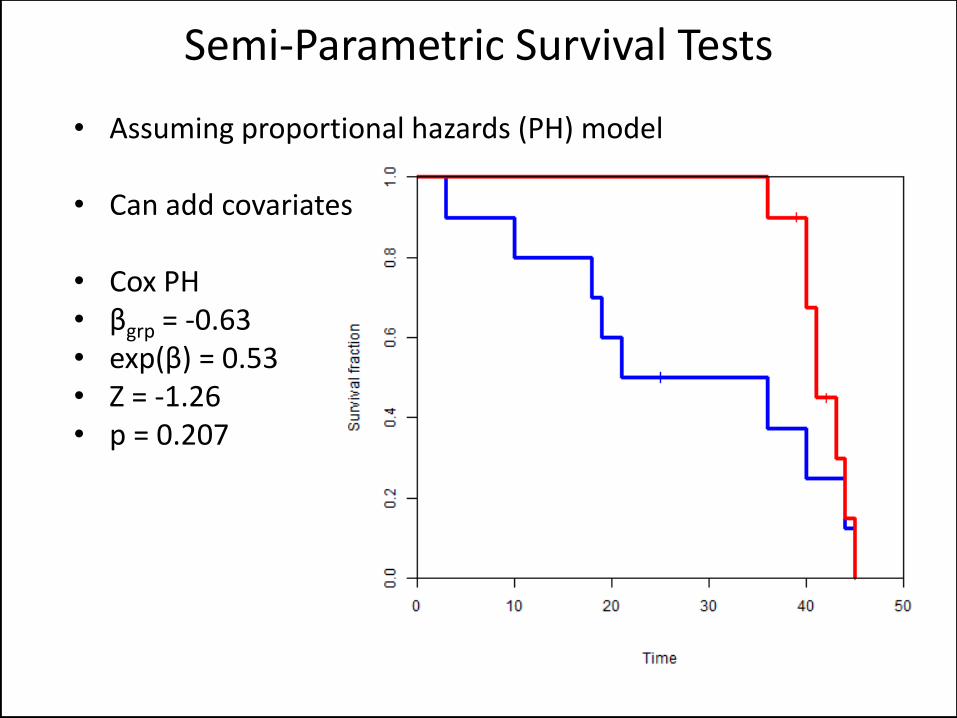
• Assuming proportional hazards (PH) model
• Can add covariates
• Cox PH • βgrp = -0.63 • exp(β) = 0.53 • Z = -1.26 • p = 0.207
Semi-Parametric Survival Tests
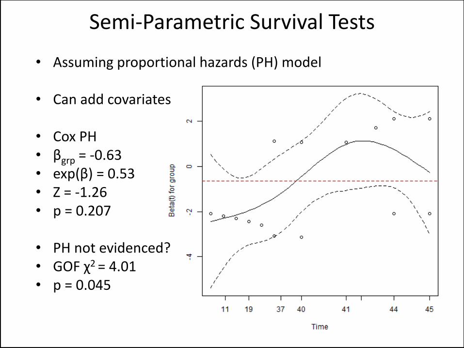
• Assuming proportional hazards (PH) model
• Can add covariates
• Cox PH • βgrp = -0.63 • exp(β) = 0.53 • Z = -1.26 • p = 0.207
• PH not evidenced? • GOF χ2 = 4.01 • p = 0.045
Semi-Parametric Survival Tests
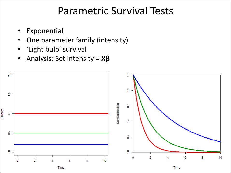
• Exponential • One parameter family (intensity) • ‘Light bulb’ survival • Analysis: Set intensity = Xβ
Parametric Survival Tests
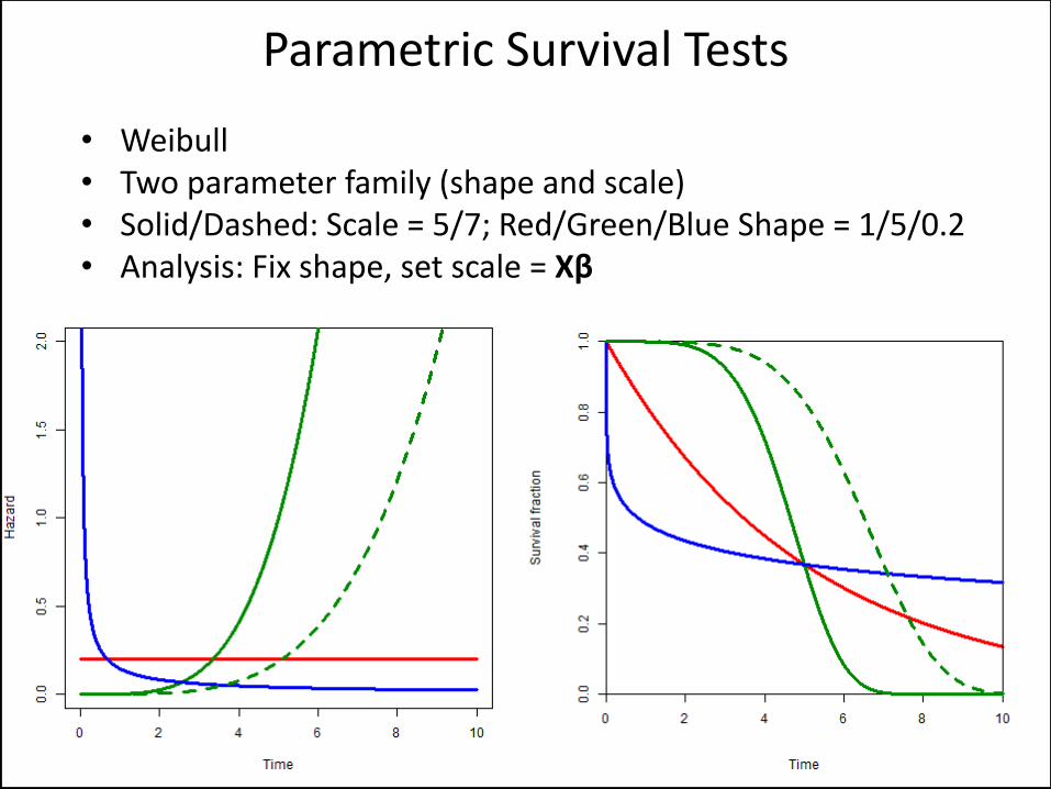
• Weibull • Two parameter family (shape and scale) • Solid/Dashed: Scale = 5/7; Red/Green/Blue Shape = 1/5/0.2 • Analysis: Fix shape, set scale = Xβ
Parametric Survival Tests
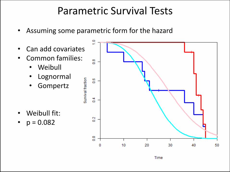
• Assuming some parametric form for the hazard
• Can add covariates • Common families:
• Weibull • Lognormal • Gompertz
• Weibull fit: • p = 0.082
Parametric Survival Tests
Section Summary
• Account for censoring in the data • Most people will use NP or SP methods, even if the
underlying assumptions are not evidenced • Parametric models must be rigorously checked
• And then justified
• First step: Look at the (KM) survival curves
• Any time-to-event analysis that does not present KM estimates of the survival curves is not to be trusted. Period.

Thank You
Questions before the discussion?