Statistical Analysis of PEM Life Test Data

Implications for PEM Usage in High Reliability Long Duration Space Missions

Extracting More Information Electrical Parameters Measurements During Life Testing

Purpose

• Review analyses performed so far• Suggest additional work (analysis)

Purpose of Life Testing• “Mimics” early mission usage

– Accelerates failures and parameter changes by employing high junction temperature

• Mission failure probability is reduced by transferring flight parts to lower failure rate region

– Burn-in– Assumes (without test) decreasing failure rate applies to early mission usage

• Life test validates infant mortals removed from flight population with known confidence (Chi-square distribution)

• Life test sample size (woefully) inadequate to demonstrate long term failure rate

• Some projects (Minuteman) removed from flight population parts “drifting” – Electrical parameters selected arbitrarily – Criteria for removal is qualitative– Technical literature does not contain objective assessment of validity of this

technique• What can be objectively “squeezed” out of life test data electrical

parameter changes and what does it mean?

Method to Assess PEM Life Test Data

• Measure all electrical parameters feasible across industrial temperature range• Measure interim values (during course of life test)• Plot electrical parameters on probability scales

– Evaluate parameters that change significantly (standard deviation is at least 10% of part manufacturer specification) (Significance Test)

– Initial, post-burn-in, interim measurements (as available), final measurements• Curve fit experimental data to known statistical distributions

– Normal– Student t– Log normal– Bimodal– Etc.

• Use known characteristics of these statistical distributions to estimate RANGE• Perform longitudinal analysis

– Look at predicted range during the course of life tests– If the predicted range is stable compare to parts manufacturer specification limits– Remember manufacturer limits are not determined by statistical criteria

• Typically marketing considerations are more important

• Review circuit applications with CogE to ensure circuit error budget can tolerate Range (so computed) to an acceptable confidence level

– Use JPL-D8545 as initial guide

Formulas from Statistics

Facts about Statistical Distributions

• Distributions that fit experimental PEM life test data are typically central– Average less than standard deviation

• Normal distribution has lean tails– Population falls off rapidly after a few standard deviations

• Student t distribution can describe experimental data with fat tails– Less rapid falloff of population– Rate of falloff dependent on degrees of freedom used to curve fit– Range is larger than normal distribution

• Both distributions do not have skew– Distributions symmetrical around average

• Range is maximum minus minimum value measured– For a distribution that fits experimental data, range may be predicted from

standard deviation, sample size (number of parts used in circuit), and probability (in this case, similar to confidence level)

Range of Normal Distribution (W)

Sample Size (n) W (90%) W(99%)

5 3.48 4.60

10 4.13 5.16

20 4.69 5.65

Student t Distribution Plotted on Probability Scale

Student t Distribution

Degrees of Freedom (f) Standard Deviation

10 1.05

5 1.12

4 1.15

2 1.41

)3

1(f

Wq

Studentized Range

Examples

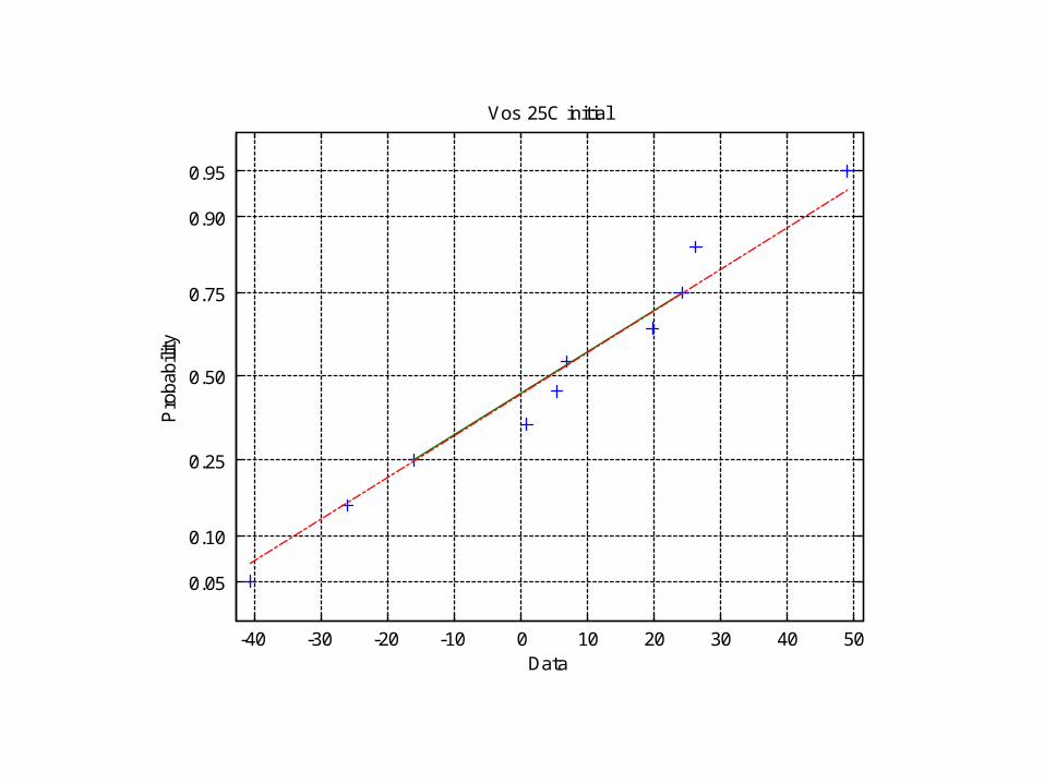
LT1028• Ultra low noise, high speed, operational amplifier• 10 piece life test sample measured at 500 and 1000 hours of life

test• Vos (input offset voltage) at 1000 hours and room and cold temp

and Ib (input bias current) at 1000 hours and room temp had changes whose standard deviation was significant

• I also show some open loop gain data– Open loop gain should not be used in good circuit design– Circuits should employ substantial negative feedback

• MATLAB used to plot experimental data on probability scales

-40 -30 -20 -10 0 10 20 30 40 50

0.05

0.10

0.25

0.50

0.75

0.90

0.95

Data

Pro

babi

lity

Vos 25C initial

-50 -40 -30 -20 -10 0 10 20 30

0.05

0.10

0.25

0.50

0.75

0.90

0.95

Data

Pro

babi

lity

Vos 25C post burn-in

-40 -30 -20 -10 0 10 20 30 40

0.05

0.10

0.25

0.50

0.75

0.90

0.95

Data

Pro

babi

lity

Vos 25 C 500 hours

-40 -30 -20 -10 0 10 20 30 40 50

0.05

0.10

0.25

0.50

0.75

0.90

0.95

Data

Pro

babi

lity

Vos 25C 1000 hours

Voltage Offset 25C

Average Standard Deviation

Predicted Range (10 parts; 99% probability)

Manufacturer Limits

Initial 5.0 27 139 +/- 80

Post burn-in -6.1 28 144 +/- 80

500 hours 2.2 28 144 +/- 80

1000 hours 3.4 29 149 +/- 80

-60 -50 -40 -30 -20 -10 0 10 20 30 40

0.05

0.10

0.25

0.50

0.75

0.90

0.95

Data

Pro

babi

lity

Vos -40C Initial

-80 -60 -40 -20 0 20

0.05

0.10

0.25

0.50

0.75

0.90

0.95

Data

Pro

babi

lity

Vos -40C Post Burn-in

-40 -20 0 20 40 60

0.05

0.10

0.25

0.50

0.75

0.90

0.95

Data

Pro

babi

lity

Vos -40C 500 hours

-80 -60 -40 -20 0 20 40

0.05

0.10

0.25

0.50

0.75

0.90

0.95

Data

Pro

babili

ty

Vos -40C 1000 hours

Voltage Offset at -40C

Average Standard Deviation

Predicted Range (10 parts; 99% probability)

Manufacturer Limits

Initial -14 35 178 +/- 150

Post burn-in -24 37 192 +/- 150

500 hours 2.0 38 195 +/- 150

1000 hours 26 47 244 +/- 150

-50 -40 -30 -20 -10 0 10 20 30

0.05

0.10

0.25

0.50

0.75

0.90

0.95

Data

Pro

babi

lity

IB 25C Initial

-60 -50 -40 -30 -20 -10 0 10 20

0.05

0.10

0.25

0.50

0.75

0.90

0.95

Data

Pro

babi

lity

Ib 25C Post Burn in

-70 -60 -50 -40 -30 -20 -10 0 10 20 30

0.05

0.10

0.25

0.50

0.75

0.90

0.95

Data

Pro

babi

lity

Ib 25C 500 hours

-80 -70 -60 -50 -40 -30 -20 -10 0 10 20

0.05

0.10

0.25

0.50

0.75

0.90

0.95

Data

Pro

babili

ty

Ib 25C 1000 hours

Input Bias Current 25C

Average Standard Deviation

Predicted Range (10 parts; 99% probability)

Manufacturer Limits

Initial -0.2 31 162 +/- 90

Post burn-in -5.1 33 172 +/- 90

500 hours 7.4 34 175 +/- 90

1000 hours 18 36 188 +/- 90

20 40 60 80 100 120 140 160 180

0.05

0.10

0.25

0.50

0.75

0.90

0.95

Data

Pro

babi

lity

Gain 25C 500 hours

1 1.2 1.4 1.6 1.8 2 2.2

0.05

0.10

0.25

0.50

0.75

0.90

0.95

Data

Pro

babi

lity

Log Gain 25C 500 hours

20 40 60 80 100 120

0.05

0.10

0.25

0.50

0.75

0.90

0.95

Data

Pro

babili

ty

Gain 25C 1000 hours

1 1.2 1.4 1.6 1.8 2

0.05

0.10

0.25

0.50

0.75

0.90

0.95

Data

Pro

bability

Log Gain 25C 1000 hours

Assessment

• Input offset voltage fits normal distribution (25C and -40C)• Input bias current fits normal distribution (25C) • (FYI) Log Open loop gain fits normal distribution better than open

loop gain– e.g. open loop gain fits log normal distribution

• Critical application parameters fit within part manufacturer specified range to high confidence

LT1813

• Dual high speed very high slew rate operational amplifier• 22 piece life test sample measured at 1000 hours • Vos (input offset voltage) at 1000 hours (25C) and Iio (input offset

current) at 1000 hours (25C) had changes whose standard deviation was significant

• MATLAB used to plot experimental data on probability scales

-0.5 0 0.5 1

0.02

0.05

0.10

0.25

0.50

0.75

0.90

0.95

0.98

Data

Pro

bability

Vos 25C Initial

-0.2 0 0.2 0.4 0.6 0.8 1

0.02

0.05

0.10

0.25

0.50

0.75

0.90

0.95

0.98

Data

Pro

bability

Vos 25C Post Burn In

-0.4 -0.2 0 0.2 0.4 0.6 0.8 1

0.02

0.05

0.10

0.25

0.50

0.75

0.90

0.95

0.98

Data

Pro

babili

ty

Vos 25C 1000 hours

Input Voltage Offset (25C)

Average Standard Deviation

Predicted Range (10 parts; 99% probability)

Manufacturer Limits

Initial 0.34 0.38 1.9 +/- 1.5

Post burn-in 0.47 0.37 1.9 +/- 1.5

1000 hours 0.34 0.38 1.96 +/- 1.5

-15 -10 -5 0 5 10 15

0.02

0.05

0.10

0.25

0.50

0.75

0.90

0.95

0.98

Data

Pro

babili

tyIio 25C Initial

-15 -10 -5 0 5 10 15

0.02

0.05

0.10

0.25

0.50

0.75

0.90

0.95

0.98

Data

Pro

babili

ty

Iio 25C Post Burn In

-15 -10 -5 0 5 10 150.01

0.02

0.05

0.10

0.25

0.50

0.75

0.90

0.95

0.98

0.99

Data

Pro

bability

Iio 25C 1000 hours

Input Offset Current (25C)

Average Standard Deviation

Predicted Range (10 parts; 99% probability)

Manufacturer Limits

Initial 1.7 8.7 45 +/- 400

Post burn-in 1.5 8.8 45 +/- 400

1000 hours 1.9 9.0 46 +/- 400

Assessment

• Parameters well fit to normal distribution• Ranges within part manufacturer data sheet

limits to high confidence• Most parameters changed very little

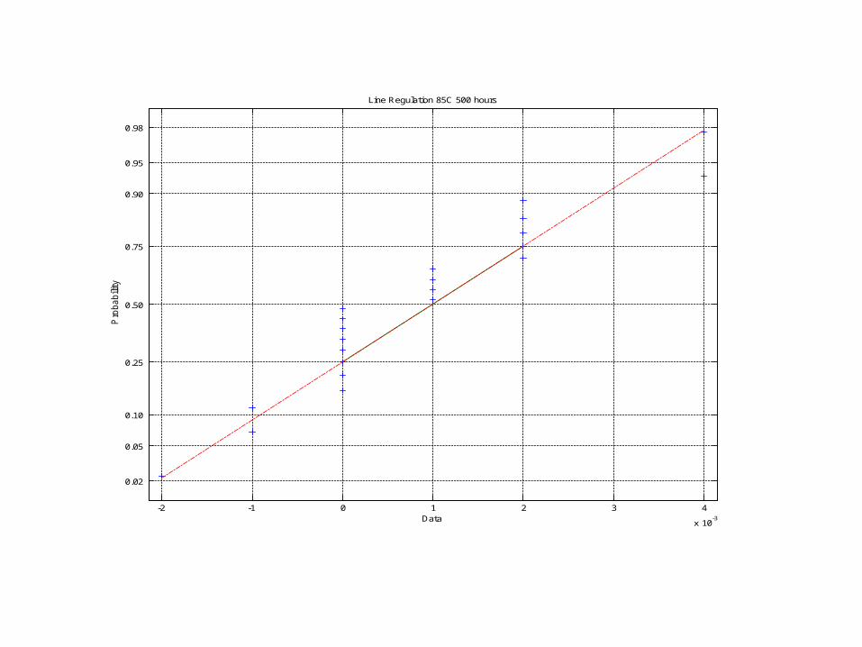
LT1175

• Negative low dropout micropower voltage regulator• 22 piece life test with measurements at 500 and 2000 hours• Parameters with significnat changes include line regulation, load

regulation, sense current• Only parameters with greatest changes are shown in this

presentation• MATLAB was used to plot experimental data on probability scales

-1 -0.5 0 0.5 1 1.5 2 2.5 3 3.5 4

x 10-3

0.02

0.05

0.10

0.25

0.50

0.75

0.90

0.95

0.98

Data

Pro

bability

Line Regulation 85C Initial

-2 -1 0 1 2 3 4

x 10-3

0.02

0.05

0.10

0.25

0.50

0.75

0.90

0.95

0.98

Data

Pro

babili

ty

Line Regulation 85C 500 hours

-0.06 -0.04 -0.02 0 0.02 0.04 0.06 0.08 0.1

0.02

0.05

0.10

0.25

0.50

0.75

0.90

0.95

0.98

Data

Pro

bability

Line Regulation 85C 2000 hours

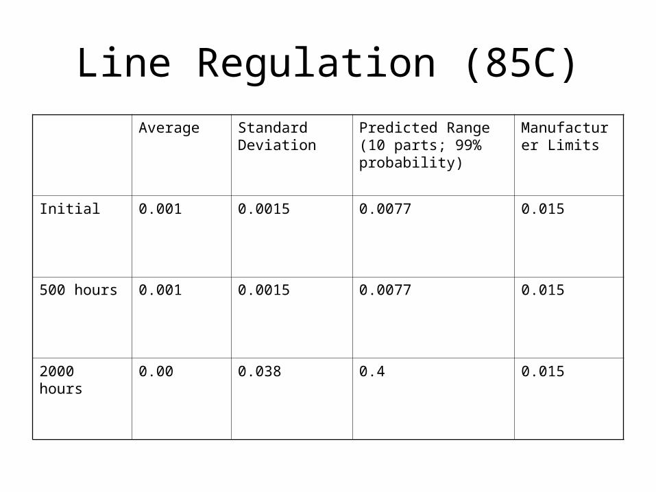
Line Regulation (85C)

Average Standard Deviation

Predicted Range (10 parts; 99% probability)

Manufacturer Limits

Initial 0.001 0.0015 0.0077 0.015

500 hours 0.001 0.0015 0.0077 0.015

2000 hours 0.00 0.038 0.4 0.015

-0.2 -0.15 -0.1 -0.05 0 0.05 0.1 0.15 0.2 0.25 0.3

0.02

0.05

0.10

0.25

0.50

0.75

0.90

0.95

0.98

Data

Pro

bability

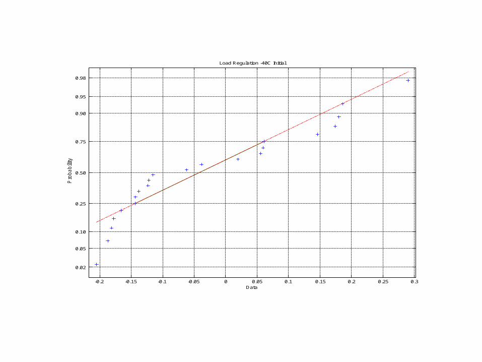
Load Regulation -40C Initial

-0.25 -0.2 -0.15 -0.1 -0.05 0 0.05 0.1 0.15 0.2

0.02

0.05

0.10

0.25

0.50

0.75

0.90

0.95

0.98

Data

Pro

bability

Load Regulation -40C 500 hours

-0.45 -0.4 -0.35 -0.3 -0.25 -0.2 -0.15 -0.1 -0.05 0

0.02

0.05

0.10

0.25

0.50

0.75

0.90

0.95

0.98

Data

Pro

babili

ty

Load Regulation -40C 2000 hours

Load Regulation (-40C)

Average Standard Deviation

Predicted Range (10 parts; 99% probability)

Manufacturer Limits

Initial =0.29 0.15 0.78 0.035

500 hours 0.019 0.12 0.61 0.035

2000 hours -0.18 0.12 0.63 0.035

20 30 40 50 60 70 80 90

0.02

0.05

0.10

0.25

0.50

0.75

0.90

0.95

0.98

Data

Pro

bability

Sense Current 85C Initial

10 20 30 40 50 60 70 80

0.02

0.05

0.10

0.25

0.50

0.75

0.90

0.95

0.98

Data

Pro

bability

Sense Current 85C 500 hours

0.098 0.1 0.102 0.104 0.106 0.108 0.11

0.02

0.05

0.10

0.25

0.50

0.75

0.90

0.95

0.98

Data

Pro

bability

Sense Current 85C 2000 hours

Sense Current 85C

Average Standard Deviation

Predicted Range (10 parts; 99% probability)

Manufacturer Limits

Initial 58 19 101 150

500 hours 43 22 111 150

2000 hours 0.1 0.004 0.02 150

2000 hour data was reviewed and is bad at both temperature extremes

Assessment

• Line regulation (85C) fits normal distribution except at 2000 hours where the fat tails require a student t fit with 3 degrees of freedom

• Load regulation (-40C) fits normal distribution• Sense current (85C) fits normal distribution except 2000 hour data is corrupt• Extra derating is needed for circuit applications at temperature extremes• Distributions at room temperature are well fitted to normal distribution and

have less predicted range

AD780BR• High Precision (Band Gap) Voltage Reference• 49 devices subjected to life test and measured at 250 hours, 500

hours, 1000 hours• Output voltage (3V nom) had significant standard deviation of the

change at -40C and 250 hours• Load regulation (sink mode B) had significant standard deviation of

change at 25C and 500 hours; output voltage at 85C and 500 hours• Load regulation (sink mode B) had significant standard deviation of

changes at four temperatures and 1000 hours; output voltage at 125C/85C/-40C and 1000 hours and load regulation (sink mode A) load regulation (shunt mode) at 125C/-40C and 1000 hours

• MATLAB used to plot changes for significant recurring parameters

2.9992.99922.99942.99962.9998 3 3.00023.00043.00063.00083.001

0.01 0.02

0.05

0.10

0.25

0.50

0.75

0.90

0.95

0.98 0.99

Data

Pro

babili

ty

Output Voltage 3V nom 85C Initial

2.999 2.9992 2.9994 2.9996 2.9998 3 3.0002 3.0004 3.0006 3.0008

0.01 0.02

0.05

0.10

0.25

0.50

0.75

0.90

0.95

0.98 0.99

Data

Pro

babili

tyOutput Voltage 3V nom 85C Post burn-in

2.9992 2.9994 2.9996 2.9998 3 3.0002 3.0004 3.0006 3.0008

0.01 0.02

0.05

0.10

0.25

0.50

0.75

0.90

0.95

0.98 0.99

Data

Pro

babili

ty

Output Voltage 3V nom 85C 250 hours

2.9992 2.9994 2.9996 2.9998 3 3.0002 3.0004 3.0006 3.0008 3.001

0.01 0.02

0.05

0.10

0.25

0.50

0.75

0.90

0.95

0.98 0.99

Data

Pro

babili

tyOutput Voltage 3V nom 85C 500 hours

2.99862.9988 2.999 2.99922.99942.99962.9998 3 3.00023.00043.0006

0.01 0.02

0.05

0.10

0.25

0.50

0.75

0.90

0.95

0.98 0.99

Data

Pro

babili

tyOutput Voltage 3V nom 85C 1000 hours

Output Voltage (3V nom) (85C)

Average Standard Deviation

Predicted Range (10 parts; 99% probability)

Manufacturer Limits

Initial 2.9998 0.00045 0.0023 +/- 0.001

Post Burn-in 2.9997 0.00045 0.0023 +/- 0.001

250 hours 2.9998 0.00039 0.0020 +/- 0.001

500 hours 2.9999 0.0004 0.0022 +/- 0.001

1000 hours 2.9993 0.0004 0.0021 +/- 0.001

-0.05 0 0.05 0.1 0.15 0.2 0.25 0.3

0.01 0.02

0.05

0.10

0.25

0.50

0.75

0.90

0.95

0.98 0.99

Data

Pro

babi

lity

Load Regulation Sink Mode B 25C 500 hours

-2 -1.5 -1 -0.50.01

0.02

0.05

0.10

0.25

0.50

0.75

0.90

0.95

0.98

0.99

Data

Pro

babili

ty

Log Norm Plot Reg Sink Mode B 25C 500 hours

-0.05 0 0.05 0.1 0.15 0.2 0.25

0.01 0.02

0.05

0.10

0.25

0.50

0.75

0.90

0.95

0.98 0.99

Data

Pro

babi

lity

Load Regulation Sink Mode B 25C 1000 hours

-2 -1.8 -1.6 -1.4 -1.2 -1 -0.8 -0.6

0.02

0.05

0.10

0.25

0.50

0.75

0.90

0.95

0.98

Data

Pro

babi

lity

Log Norm Plot Reg Sink Mode B 25C 1000 hours

Load Regulation Sink Mode B (25C)

Average Standard Deviation

Predicted Range (10 parts; 99% probability)

Predicted Range (log normal fit)

Manufacturer Limits

Initial 0.007 0.057 0.29 * 0.75

Post Burn-in 0.027 0.046 0.24 0.75

250 hours 0.017 0.038 0.19 0.75

500 hours 0.021 0.060 0.31* 0.75

1000 hours 0.022 0.062 0.32 * 0.75

* Log normal fit to positive values is better fit

Assessment

• Load regulation (sink mode B) (25C) fits normal distribution – Outlier analysis may require bimodal fit– Significant outliers only at initial and 1000 hour points

• Output voltage (3V nominal) fits normal distribution• Other parameters had smaller changes during life test• Output voltage (2.5V nominal) showed small changes; however 3V

nom output voltage requires derating in circuit application• Load regulations are within part manufacturer specified ranges

AD8028

• Low Distortion Dual Rail to Rail Operational Amplifier

• 10 pieces tested after burn-in (herein identified as initial measurements), after 500 hours life test, after 1000 hours life test.

• This is a dual device, and, where applicable, measurements on same parameters combined to increase sample size for statistical validity improvement

• Measurements were taken at 25C, +110C, -40C.

-0.8 -0.7 -0.6 -0.5 -0.4 -0.3

0.02

0.05

0.10

0.25

0.50

0.75

0.90

0.95

0.98

Data

Pro

babi

lity

Vos 110C Initial

-0.75 -0.7 -0.65 -0.6 -0.55 -0.5 -0.45 -0.4 -0.35 -0.3 -0.25

0.02

0.05

0.10

0.25

0.50

0.75

0.90

0.95

0.98

Data

Pro

babi

lity

Vos 110C 500 hours

-0.75 -0.7 -0.65 -0.6 -0.55 -0.5 -0.45 -0.4 -0.35 -0.3

0.02

0.05

0.10

0.25

0.50

0.75

0.90

0.95

0.98

Data

Pro

babi

lity

Vos 110C 1000 hours

Initial 500 hours 1000 hours

Average -0.484 -0.461 -0.457

Standard Deviation 0.154073 0.142465 0.138103

Predicted Range 0.795017 0.73512 0.712613

Note: Input Offset voltage specified at 25C as 0.8 millivolts max. No specification at temperature extremes.Measurements hardly changed at all during life test.

ISL43110

• Low-Voltage, Single Supply, SPST, High Performance Analog Switches

• 48 pieces were tested initially and after 80 hours, 160 hours of burn-in and 240 hours of burn-in

• Typical circuit critical parameters are On resistance, On resistance flatness, various leakage currents.

• Measurements were taken at 25°C, -40°C and +85°C.

11 11.5 12 12.5 13 13.5 14 14.5 15 15.5 16

0.01 0.02

0.05

0.10

0.25

0.50

0.75

0.90

0.95

0.98 0.99

Data

Pro

babi

lity

Ron 25C Initial

11 11.5 12 12.5 13 13.5 14 14.5 15 15.5 16

0.01 0.02

0.05

0.10

0.25

0.50

0.75

0.90

0.95

0.98 0.99

Data

Pro

babi

lity

Ron 25C 80 hours of burn-in

11 11.5 12 12.5 13 13.5 14 14.5 15 15.5 16

0.01 0.02

0.05

0.10

0.25

0.50

0.75

0.90

0.95

0.98 0.99

Data

Pro

babi

lity

Ron 25C 160 hours burn-in

11 11.5 12 12.5 13 13.5 14 14.5 15 15.5 16

0.01 0.02

0.05

0.10

0.25

0.50

0.75

0.90

0.95

0.98 0.99

Data

Pro

babi

lity

Ron 25C 240 hours of burn-in

Ron 25C statistical values after 80 hours burn-in

Average 12.858 15.706 11.269 11.587

Standard deviation 0.176851 0.120816 0.127684 0.154643

Predicted range 0.912552 0.623411 0.658847 0.797956

Ron 25C statistical values after 160 hours burn-in

Average 12.935 15.756 11.341 11.665

Standard deviation 0.17158 0.100202 0.123671 0.15427

Predicted range 0.885351 0.517041 0.638144 0.796035

Ron 25C statistical values after 240 hours burn-in

Average 12.943 15.803 11.365 11.681

Standard deviation 0.207219 0.127929 0.154025 0.184966

Predicted range 1.069252 0.660114 0.794768 0.954427

Distributions are reasonably matched to normal. Small changes observed in average and standard deviations. Predicted range in all cases was less than 1.1 ohm. Vendor datasheet specified maximum is 20 ohms at 25C. Therefore statistical scatter is small and remains so for the population throughout the burn-in.

General Conclusions

• Performing statistical analysis to actual experimental data showed the large majority of data is well fitted to normal distribution

• Most parameters have predicted range within part manufacturer datasheet specified range– Some parameters require derating in circuit application depending on

quantity of parts used and confidence levels required

• Some experimental data is suspect and tests should be repeated if feasible

• It is recommended that an analysis of the accuracy of experimental measurements be made in all cases so there is more confidence in validity of test data