Statistical Analysis of List Experimentsimai.princeton.edu/research/files/listP.pdfStatistical...
31
Political Analysis (2012) 20:47−77 doi:10.1093/pan/mpr048 Statistical Analysis of List Experiments Graeme Blair and Kosuke Imai Department of Politics, Princeton University, Princeton, NJ 08544 e-mail: [email protected]; [email protected] (corresponding authors) Edited by R. Michael Alvarez The validity of empirical research often relies upon the accuracy of self-reported behavior and beliefs. Yet eliciting truthful answers in surveys is challenging, especially when studying sensitive issues such as racial prejudice, corruption, and support for militant groups. List experiments have attracted much attention recently as a potential solution to this measurement problem. Many researchers, however, have used a simple difference-in-means estimator, which prevents the efficient examination of multivariate relationships between respondents’ characteristics and their responses to sensitive items. Moreover, no systematic means exists to investigate the role of underlying assumptions. We fill these gaps by developing a set of new statistical methods for list experiments. We identify the commonly invoked assumptions, propose new multivariate regression estimators, and develop methods to detect and adjust for potential violations of key assumptions. For empirical illustration, we analyze list experiments concerning racial prejudice. Open-source software is made available to implement the proposed methodology. 1 Introduction The validity of much empirical social science research relies upon the accuracy of self-reported individ- ual behavior and beliefs. Yet eliciting truthful answers in surveys is challenging, especially when studying such sensitive issues as racial prejudice, religious attendance, corruption, and support for militant groups (e.g., Kuklinski, Cobb, and Gilens 1997a; Presser and Stinson 1998; Gingerich 2010; Bullock, Imai, and Shapiro 2011). When asked directly in surveys about these issues, individuals may conceal their actions and opinions in order to conform to social norms or they may simply refuse to answer the questions. The potential biases that result from social desirability and nonresponse can seriously undermine the credi- bility of self-reported measures used by empirical researchers (Berinsky 2004). In fact, the measurement problem of self-reports can manifest itself even for seemingly less sensitive matters such as turnout and media exposure (e.g., Burden 2000; Zaller 2002). The question of how to elicit truthful answers to sensitive questions has been a central methodological challenge for survey researchers across disciplines. Over the past several decades, various survey tech- niques, including the randomized response method, have been developed and used with a mixed record of success (Tourangeau and Yan 2007). Recently, list experiments have attracted much attention among social scientists as an alternative survey methodology that offers a potential solution to this measure- ment problem (e.g., Kuklinski, Cobb, and Gilens 1997a; Kuklinski et al. 1997b; Sniderman and Carmines 1997; Gilens, Sniderman, and Kuklinski 1998; Kane, Craig, and Wald 2004; Tsuchiya, Hirai, and Ono 2007; Streb et al. 2008; Corstange 2009; Flavin and Keane 2009; Glynn 2010; Gonzalez-Ocantos et al. Authors’ note: Financial support from the National Science Foundation (SES-0849715) is acknowledged. All the proposed methods presented in this paper are implemented as part of the R package, “list: Statistical Methods for the Item Count Technique and List Experiment,” which is freely available for download at http://cran.r-project.org/package=list (Blair and Imai 2011a). The replication archive is available as Blair and Imai (2011b), and the Supplementary Materials are posted on the Political Analysis Web site. We thank Dan Corstange for providing his computer code, which we use in our simulation study, as well as for useful comments. Detailed comments from the editor and two anonymous reviewers significantly im- proved the presentation of this paper. Thanks also to Kate Baldwin, Neal Beck, Will Bullock, Stephen Chaudoin, Matthew Creighton, Michael Donnelly, Adam Glynn, Wenge Guo, John Londregan, Aila Matanock, Dustin Tingley, Teppei Yamamoto, and seminar participants at New York University, the New Jersey Institute of Technology, and Princeton University for helpful discussions. c The Author 2012. Published by Oxford University Press on behalf of the Society for Political Methodology. All rights reserved. For Permissions, please email: [email protected] 47 at Princeton University on January 18, 2012 http://pan.oxfordjournals.org/ Downloaded from
Transcript of Statistical Analysis of List Experimentsimai.princeton.edu/research/files/listP.pdfStatistical...

Political Analysis(2012) 20:47−77doi:10.1093/pan/mpr048
Statistical Analysis of List Experiments
GraemeBlair and Kosuke ImaiDepartment of Politics, Princeton University, Princeton, NJ 08544
e-mail: [email protected]; [email protected] (corresponding authors)
Editedby R. Michael Alvarez
The validity of empirical research often relies upon the accuracy of self-reported behavior and beliefs.Yet eliciting truthful answers in surveys is challenging, especially when studying sensitive issues such asracial prejudice, corruption, and support for militant groups. List experiments have attracted much attentionrecently as a potential solution to this measurement problem. Many researchers, however, have used asimple difference-in-means estimator, which prevents the efficient examination of multivariate relationshipsbetween respondents’ characteristics and their responses to sensitive items. Moreover, no systematicmeans exists to investigate the role of underlying assumptions. We fill these gaps by developing a setof new statistical methods for list experiments. We identify the commonly invoked assumptions, proposenew multivariate regression estimators, and develop methods to detect and adjust for potential violationsof key assumptions. For empirical illustration, we analyze list experiments concerning racial prejudice.Open-source software is made available to implement the proposed methodology.
1 Intr oduction
The validity of much empirical social science research relies upon the accuracy of self-reported individ-ual behavior and beliefs. Yet eliciting truthful answers in surveys is challenging, especially when studyingsuch sensitive issues as racial prejudice, religious attendance, corruption, and support for militant groups(e.g.,Kuklinski, Cobb, and Gilens 1997a; Presser and Stinson 1998;Gingerich 2010;Bullock, Imai, andShapiro 2011). When asked directly in surveys about these issues, individuals may conceal their actionsand opinions in order to conform to social norms or they may simply refuse to answer the questions. Thepotential biases that result from social desirability and nonresponse can seriously undermine the credi-bility of self-reported measures used by empirical researchers (Berinsky 2004). In fact, the measurementproblem of self-reports can manifest itself even for seemingly less sensitive matters such as turnout andmedia exposure (e.g.,Burden 2000;Zaller 2002).
The question of how to elicit truthful answers to sensitive questions has been a central methodologicalchallenge for survey researchers across disciplines. Over the past several decades, various survey tech-niques, including the randomized response method, have been developed and used with a mixed recordof success (Tourangeau and Yan 2007). Recently, list experiments have attracted much attention amongsocial scientists as an alternative survey methodology that offers a potential solution to this measure-ment problem (e.g.,Kuklinski, Cobb, and Gilens 1997a; Kuklinski et al. 1997b;Sniderman and Carmines1997;Gilens, Sniderman, and Kuklinski 1998; Kane, Craig, and Wald 2004; Tsuchiya, Hirai, and Ono2007;Streb et al. 2008; Corstange 2009; Flavin and Keane 2009;Glynn 2010; Gonzalez-Ocantos et al.
Authors’ note: Financial support from the National Science Foundation (SES-0849715) is acknowledged. All the proposedmethods presented in this paper are implemented as part of the R package, “list: Statistical Methods for the Item CountTechnique and List Experiment,” which is freely available for download athttp://cran.r-project.org/package=list(Blair andImai 2011a). The replication archive is available asBlair and Imai (2011b), and the Supplementary Materials are posted onthe Political AnalysisWeb site. We thank Dan Corstange for providing his computer code, which we use in our simulationstudy, as well as for useful comments. Detailed comments from the editor and two anonymous reviewers significantly im-proved the presentation of this paper. Thanks also to Kate Baldwin, Neal Beck, Will Bullock, Stephen Chaudoin, MatthewCreighton, Michael Donnelly, Adam Glynn, Wenge Guo, John Londregan, Aila Matanock, Dustin Tingley, Teppei Yamamoto,and seminar participants at New York University, the New Jersey Institute of Technology, and Princeton University for helpfuldiscussions.
c© TheAuthor 2012. Published by Oxford University Press on behalf of the Society for Political Methodology.All rights reserved. For Permissions, please email: [email protected]
47
at Princeton University on January 18, 2012
http://pan.oxfordjournals.org/D
ownloaded from

48 GraemeBlair and Kosuke Imai
2010;Holbrookand Krosnick 2010; Janus 2010;Redlawsk, Tolbert, and Franko 2010; Coutts and Jann2011;Imai 2011).1 A growing number of researchers are currently designing and analyzing their own listexperiments to address research questions that are either difficult or impossible to study with direct surveyquestions.
The basic idea of list experiments is best illustrated through an example. In the 1991 National Raceand Politics Survey, a group of political scientists conducted the first list experiment in the discipline(Sniderman, Tetlock, and Piazza 1992). In order to measure racial prejudice, the investigators randomlydivided the sample of respondents into treatment and control groups and asked the following question forthe control group:
Now I’m going to read you three things that sometimes make peopleangry or upset. After I read all three, just tell me HOW MANY ofthem upset you. (I don’t want to know which ones, just how many.)
(1) the federal government increasing the tax on gasoline
(2) professional athletes getting million-dollar-plus salaries
(3) large corporations polluting the environment
How many, if any, of these things upset you?
For the treatment group, they asked an identical question except that a sensitive item concerning racialprejudice was appended to the list,
Now I’m going to read you four things that sometimes make peopleangry or upset. After I read all four, just tell me HOW MANY ofthem upset you. (I don’t want to know which ones, just how many.)
(1) the federal government increasing the tax on gasoline
(2) professional athletes getting million-dollar-plus salaries
(3) large corporations polluting the environment
(4) a black family moving next door to you
How many, if any, of these things upset you?
The premise of list experiments is that if a sensitive question is asked in this indirect fashion, respon-dents may be more willing to offer a truthful response even when social norms encourage them to answerthe question in a certain way. In the example at hand, list experiments may allow survey researchers toelicit truthful answers from respondents who do not wish to have a black family as a neighbor but areaware of the commonly held equality norm that blacks should not be discriminated against based on theirethnicity. The methodological challenge, on the other hand, is how to efficiently recover truthful responsesto the sensitive item from aggregated answers in response to indirect questioning.
Despite their growing popularity, statistical analyses of list experiments have been unsatisfactory fortwo reasons. First, most researchers have relied upon the difference in mean responses between thetreatment and control groups to estimate the population proportion of those respondents who answerthe sensitive item affirmatively.2 The lack of multivariate regression estimators made it difficult to effi-ciently explore the relationships between respondents’ characteristics and their answers to sensitive items.Although some have begun to apply multivariate regression techniques such as linear regression withinteraction terms (e.g.,Holbrook and Krosnick 2010; Glynn 2010; Coutts and Jann 2011) and an
1A variant of this technique was originally proposed byRaghavarao and Federer(1979), who called it theblock total responsemethod. The method is also referred to as the item count technique (Miller 1984) or unmatched count technique (Dalton, Wimbush,and Daily 1994) and has been applied in a variety of disciplines (see, e.g.,Droitcour et al. 1991; Wimbush and Dalton 1997; LaBrieand Earleywine 2000; Rayburn, Earleywine, and Davison 2003among many others).
2Several refinements based on this difference-in-means estimator and various variance calculations have been studied in the method-ological literature (e.g.,Raghavarao and Federer 1979; Tsuchiya 2005; Chaudhuri and Christofides 2007).
at Princeton University on January 18, 2012
http://pan.oxfordjournals.org/D
ownloaded from

StatisticalAnalysis of List Experiments 49
approximatelikelihood-based model for a modified design (Corstange 2009), they are prone to bias, muchless efficient, and less generalizable than the (exact) likelihood method we propose here (see alsoImai2011).3
This state of affairs is problematic because researchers are often interested in which respondents aremore likely to answer sensitive questions affirmatively in addition to the proportion who do so. In theabove example, the researcher would like to learn which respondent characteristics are associated withracial hatred, not just the number of respondents who are racially prejudiced. The ability to adjust for mul-tiple covariates is also critical to avoid omitted variable bias and spurious correlations. Second, althoughsome have raised concerns about possible failures of list experiments (e.g.,Flavin and Keane 2009), thereexists no systematic means to assess the validity of underlying assumptions and to adjust for potentialviolations of them. As a result, it remains difficult to evaluate the credibility of empirical findings basedupon list experiments.
In this paper, we fill these gaps by developing a set of new statistical methods for list experiments.First, we identify the assumptions commonly, but often only implicitly, invoked in previous studies (Sec-tion 2.1). Second, under these assumptions, we show how to move beyond the standard difference-in-means analysis by developing new multivariate regression estimators under various designs of list exper-iments (Sections2.1–2.4). The proposed methodology provides researchers with essential tools to effi-ciently examine who is more likely to answer sensitive items affirmatively (seeBiemer and Brown 2005for an alternative approach). The method also allows researchers to investigate which respondents arelikely to answer sensitive questions differently, depending on whether asked directly or indirectly througha list experiment (Section2.2). This difference between responses to direct and indirect questioning hasbeen interpreted as a measure of social desirability bias in the list experiment literature (e.g.,Gilens,Sniderman, and Kuklinski 1998; Janus 2010).
A critical advantage of the proposed regression methodology is its greater statistical efficiency becauseit allows researchers to recoup the loss of information arising from the indirect questioning of list ex-periments.4 For example, in the above racial prejudice list experiment, using the difference-in-meansestimator, the standard error for the estimated overall population proportion of those who would answerthe sensitive item affirmatively is 0.050. In contrast, if we had obtained the same estimate using thedirect questioning with the same sample size, the standard error would have been 0.007, which is aboutseven times smaller than the standard error based on the list experiment. In addition, direct questioning ofsensitive items generally leads to greater nonresponse rates. For example, in the Multi-Investigator Sur-vey discussed in Section2.2 where the sensitive question about affirmative action is asked both directlyand indirectly, the nonresponse rate is 6.5% for the direct questioning format and 0% for the list exper-iment. This highlights the bias-variance trade-off: list experiments may reduce bias at the cost of effi-ciency.
We also investigate the scenarios in which the key assumptions break down and propose statisticalmethods to detect and adjust for certain failures of list experiments. We begin by developing a statisticaltest for examining whether responses to control items change with the addition of a sensitive item tothe list (Section3.1). Such adesign effectmay arise when respondents evaluate list items relative to oneanother. In the above example, how angry or upset respondents feel about each control item may changedepending upon whether or not the racial prejudice or affirmative action item is included in the list. Thevalidity of list experiments critically depends on the assumption of no design effect, so we propose astatistical test with the null hypothesis of no design effect. The rejection of this null hypothesis providesevidence that the design effect may exist and respondents’ answers to control items may be affected bythe inclusion of the sensitive item. We conduct a simulation study to explore how the statistical power ofthe proposed test changes according to underlying response distributions (Section3.5).
Furthermore, we show how to adjust empirical results for the possible presence ofceiling and flooreffects(Section3.2), which have long been a concern in the list experiment literature (e.g.,Kuklinski,
3For example, linear regression with interaction terms often produces negative predicted values for proportions of affirmativeresponses to sensitive items when such responses are rare.
4Appliedresearchers have used stratification and employed the difference-in-means estimator within each subset of the data definedby respondents’ characteristics of interest. The problem of this approach is that it cannot accommodate many variables or variablesthat take many different values unless a large sample is drawn.
at Princeton University on January 18, 2012
http://pan.oxfordjournals.org/D
ownloaded from

50 GraemeBlair and Kosuke Imai
Cobb,and Gilens 1997a;Kuklinski et al. 1997b). These effects represent two respondent behaviors thatmay interfere with the ability of list experiments to elicit truthful answers. Ceiling effects may result whenrespondents’ true preferences are affirmative for all the control items as well as the sensitive item. Flooreffects may arise if the control questions are so uncontroversial that uniformly negative responses areexpected for many respondents.5 Underboth scenarios, respondents in the treatment group may fear thatanswering the question truthfully would reveal their true (affirmative) preference for the sensitive item.We show how to account for these possible violations of the assumption while conducting multivariateregression analysis. Our methodology allows researchers to formally assess the robustness of their con-clusions. We also discuss how the same modeling strategy may be used to adjust for design effects(Section3.3).
For empirical illustrations, we apply the proposed methods to the 1991 National Race and PoliticsSurvey described above and the 1994 Multi-Investigator Survey (Sections2.5 and3.4). Both these sur-veys contain list experiments about racial prejudice. We also conduct simulation studies to evaluate theperformance of our methods (Sections2.6 and3.5). Open-source software, which implements all of oursuggestions, is made available so that other researchers can apply the proposed methods to their ownlist experiments. This software, “list: Statistical Methods for the Item Count Technique and List Experi-ment”(Blair and Imai 2011a), is an R package and is freely available for download at the ComprehensiveR Archive Network (CRAN;http://cran.r-project.org/package=list).
In Section4, we offer practical suggestions for applied researchers who design and analyze listexperiments. While statistical methods developed in this paper can detect and correct failures of list ex-periments under certain conditions, researchers should carefully design list experiments in order to avoidpotential violations of the underlying assumptions. We offer several concrete tips in this regard. Finally,we emphasize that the statistical methods developed in this paper, and list experiments in general, do notpermit causal inference unless additional assumptions, such as exogeneity of causal variables of interest,are satisfied. Randomization in the design of list experiments helps to elicit truthful responses to sensi-tive questions, but it does not guarantee that researchers can identify causal relationships between theseresponses and other variables.
2 Multi variate Regression Analysis for List Experiments
In this section, we show how to conduct multivariate regression analyses using the data from listexperiments. Until recently, researchers lacked methods to efficiently explore the multivariate relation-ships between various characteristics of respondents and their responses to the sensitive item (for recentadvances, seeCorstange 2009; Glynn 2010; Imai 2011). We begin by reviewing the general statisticalframework proposed byImai (2011), which allows for the multivariate regression analysis under the stan-dard design (Section2.1). We then extend this methodology to three other commonly used designs.
First, we consider the design in which respondents are also asked directly about the sensitive item afterthey answer the list experiment question about control items. This design is useful when researchers areinterested in the question of which respondents are likely to exhibit social desirability bias (Section2.2).By comparing answers to direct and indirect questioning,Gilens, Sniderman, and Kuklinski(1998) andJanus(2010) examine the magnitude of social desirability bias with respect to affirmative action andimmigration policy, respectively. We show how to conduct a multivariate regression analysis by modelingthis difference in responses as a function of respondents’ characteristics.
Second, we show how to conduct multivariate regression analysis under the design with more than onesensitive item (Section2.3). For scholars interested in multiple sensitive subjects, a common approachis to have multiple treatment lists, each of which contains a different sensitive item and the same set ofcontrol items. For example, in the 1991 National Race and Politics Survey described above, there were twosensitive items, one about a black family moving in next door and the other about affirmative action. Weshow how to gain statistical efficiency by modeling all treatment groups together with the control grouprather than analyzing each treatment group separately. Our method also allows researchers to explore therelationships between respondents’ answers to different sensitive items.
5Anotherpossible floor effect may arise if respondents fear that answering “0” reveals their truthful (negative) preference.
at Princeton University on January 18, 2012
http://pan.oxfordjournals.org/D
ownloaded from

StatisticalAnalysis of List Experiments 51
Finally, we extend this methodology to the design recently proposed byCorstange(2009) in which eachcontrol item is asked directly of respondents in the control group (Section2.4). A potential advantageof this alternative design is that it may yield greater statistical power when compared to the standarddesign because the answers to each control item are directly observed for the control group. The maindisadvantage, however, is that answers to control items may be different if asked directly than they wouldbe if asked indirectly, as in the standard design (see, e.g.,Flavin and Keane 2009; see also Section3.1fora method to detect such a design effect). Through a simulation study, we demonstrate that our proposedestimators exhibit better statistical properties than the existing estimator.
2.1 TheStandard Design
Consider the administration of a list experiment to a random sample ofN respondents from a population.Under the standard design, we randomly split the sample into treatment and control groups whereTi = 1(Ti = 0) implies that respondenti belongs to the treatment (control) group. The respondents in the controlgroup are presented with a list ofJ control items and asked how many of the items they would respond toin the affirmative. In the racial prejudice example described in Section1, three control items are used, andthus we haveJ = 3. The respondents in the treatment group are presented with the full list of one sensitiveitem andJ control items and are asked, similarly, how many of the(J + 1) items they would respond inthe affirmative to. Without loss of generality, we assume that the firstJ items, that is,j = 1, . . . , J, arecontrol items and the last item, that is,j = J + 1, is a sensitive item. The order of items on the partial andfull lists may be randomized to minimize order effects.
2.1.1 Notation
To facilitate our analysis, we use potential outcomes notation (Holland 1986) and letZi j (t) be a bi-nary variable denoting respondenti ’s preference for thej th control item for j = 1, . . . , J under thetreatment statust = 0,1. In the racial prejudice list experiment introduced in Section1, Zi 2(1) = 1meansthat respondenti would feel she is upset by the second control item—“professional athletes get-ting million-dollar-plus salaries”—when assigned to the treatment group. Similarly, we useZi,J+1(1) torepresentrespondenti ’s answer to the sensitive item under the treatment condition. The sensitive item isnot included in the control list and soZi,J+1(0) is not defined. Finally,Z∗
i j denotesrespondenti ’s truthfulanswer to thej th item wherej = 1, . . . , J + 1. In particular,Z∗
i,J+1 representsthe truthful answer to thesensitive item.
Given this notation, we further defineYi (0)=∑J
j =1 Zi j (0) andYi (1)=∑J+1
j =1 Zi j (1) asthe potentialanswer respondenti would give under the treatment and control conditions, respectively. Then, the ob-served response is represented byYi = Yi (Ti ). Note thatYi (1) takes a nonnegative integer not greater than(J + 1), while the range ofYi (0) is given by{0,1, . . . , J}. Finally, a vector of observed (pretreatment)covariates is denoted byXi ∈ X , whereX is the support of the covariate distribution. These covariatestypically include the characteristics of respondents and their answers to other questions in the survey. Therandomization of the treatment implies that potential and truthful responses are jointly independent of thetreatment variable.6
2.1.2 Identificationassumptions and analysis
We identify the assumptions commonly but often only implicitly invoked under the standard design(see alsoGlynn 2010). First, researchers typically assume that the inclusion of a sensitive item has noeffect on respondents’ answers to control items. We do not require respondents to give truthful answersto the control items. Instead, we only assume that the addition of the sensitive item does not change thesum of affirmative answers to the control items. We call this theno design effect assumptionand writeformally as,
6Formally, we write{{Z∗i j }
J+1j =1 , {Zi j (0), Zi j (1)}
Jj =1, Zi,J+1(1)} q Ti for eachi = 1, . . . ,N.
at Princeton University on January 18, 2012
http://pan.oxfordjournals.org/D
ownloaded from

52 GraemeBlair and Kosuke Imai
Table 1 An example illustrating identification under the standard design with three controlitems
Response Treatment group Control groupYi (Ti = 1) (Ti = 0)4 (3, 1)3 (2, 1) (3, 0) (3, 1) (3, 0)2 (1, 1) (2,0) (2, 1) (2, 0)1 (0, 1) (1, 0) (1, 1) (1, 0)0 (0, 0) (0, 1) (0,0)
Note. The table shows how each respondent type, characterized by(Yi (0), Z∗i,J+1), corresponds to the observed cell defined by
(Yi , Ti ), whereYi (0) representsthe total number of affirmative answers forJ control items andZ∗i,J+1 denotesthe truthful prefer-
ence for the sensitive item. In this example, the total number of control itemsJ is set to 3.
Assumption1. (No design effect). For eachi = 1, . . . ,N, we assume
J∑
j =1
Zi j (0)=J∑
j =1
Zi j (1) or equivalently Yi (1)= Yi (0)+ Zi,J+1(1).
Thesecond assumption is that respondents give truthful answers for the sensitive item. We call this theno liars assumptionand write it as follows:
Assumption 2. (No liars). For eachi = 1, . . . ,N, we assume
Zi,J+1(1)= Z∗i,J+1
whereZ∗i,J+1 representsa truthful answer to the sensitive item.
Under these two assumptions, the following standard difference-in-means estimator yields an unbiasedestimate of the population proportion of those who give an affirmative answer to the sensitive item,
τ =1
N1
N∑
i =1
Ti Yi −1
N0
N∑
i =1
(1 − Ti )Yi , (1)
whereN1 =∑N
i =1 Ti is the size of the treatment group andN0 = N − N1 is the size of the control group.7
Although this standard estimator uses the treatment and control groups separately, it is important tonote that under Assumptions1 and2, we can identify thejoint distribution of(Yi (0), Z∗
i,J+1) asshown byGlynn (2010). This joint distribution completely characterizes each respondent’s type for the purpose ofanalyzing list experiments under the standard design. For example,(Yi (0), Z∗
i,J+1) = (2,1) meansthatrespondenti affirmatively answers the sensitive item as well as two of the control items. There exist atotal of (2 × (J + 1)) such possible types of respondents.
Table 1 provides a simple example withJ = 3 that illustrates the identification of the populationproportion of each respondent type. Each cell of the table contains possible respondent types. For example,the respondents in the control group whose answer is 2, that is,Yi = 2, are either type(Yi (0), Z∗
i,J+1) =(2,1) or type (2,0). Similarly, those in the treatment group whose answer is 2 are either type(1,1) or(2,0). Since the types are known for the respondents in the treatment group withYi = 0 andYi = 4, thepopulation proportion of each type can be identified from the observed data under Assumptions1 and2.More generally, if we denote the population proportion of each type asπyz = Pr(Yi (0)= y, Z∗
i,J+1 = z)for y = 0, . . . , J andz = 0,1, thenπyz is identified for ally = 0, . . . , J as follows:
πy1 = Pr(Yi 6 y|Ti = 0)− Pr(Yi 6 y|Ti = 1), (2)
πy0 = Pr(Yi 6 y|Ti = 1)− Pr(Yi 6 y − 1|Ti = 0). (3)
7Theunbiasedness impliesE(τ ) = Pr(Z∗i,J+1 = 1).
at Princeton University on January 18, 2012
http://pan.oxfordjournals.org/D
ownloaded from

StatisticalAnalysis of List Experiments 53
2.1.3 Multivariate regression analysis
The major limitation of the standard difference-in-means estimator given in equation (1) is that itdoes not allow researchers to efficiently estimate multivariate relationships between preferences over thesensitive item and respondents’ characteristics. Researchers may apply this estimator to various subsets ofthe data and compare the results, but such an approach is inefficient and is not applicable when the samplesize is small or when many covariates must be incorporated into analysis.
To overcome this problem,Imai (2011) developed two new multivariate regression estimators underAssumptions1 and2. The first is the following nonlinear least squares (NLS) estimator:
Yi = f (Xi , γ )+ Ti g(Xi , δ)+ εi , (4)
whereE(εi |Xi , Ti ) = 0 and (γ, δ) is a vector of unknown parameters. The model puts together twopossibly nonlinear regression models, wheref (x, γ ) andg(x, δ) represent the regression models for theconditional expectations of the control and sensitive items given the covariates, respectively, wherex ∈X .8 Onecan use, for example, logistic regression submodels, which would yieldf (x, γ ) = E(Yi (0)|Xi =x) = J × logit−1(x>γ ) andg(x, δ) = Pr(Z∗
i,J+1 = 1|Xi = x) = logit−1(x>δ). Heteroskedasticity-consistent standard errors are used because the variance of error term is likely to be different between thetreatment and control groups.
This estimator includes two other important estimators as special cases. First, it generalizes thedifference-in-means estimator because the procedure yields an estimate that is numerically identical toit when Xi containsonly an intercept. Second, if linearity is assumed for the two submodels, that is,f (x, γ ) = x>γ andg(x, δ) = x>δ, then the estimator reduces to the linear regression with interactionterms (e.g.,Holbrook and Krosnick 2010; Coutts and Jann 2011),
Yi = X>i γ + Ti X>
i δ + εi . (5)
As before, heteroskedasticity-consistent robust standard errors should be used because the error variancenecessarily depends on the treatment variable. This linear specification is advantageous in that estimationand interpretation are more straightforward than the NLS estimator, but it does not take into account thefact that the response variables are bounded.
The proposed NLS estimator is consistent so long as the conditional expectation functions are correctlyspecified regardless of the exact distribution of error term.9 However, this robustness comes with a price.In particular, the estimator can be inefficient because it does not use all the information about the jointdistribution of(Yi (0), Z∗
i,J+1), which is identified under Assumptions1 and2 as shown above. To over-come this limitation,Imai (2011) proposes the maximum likelihood (ML) estimator by modeling the jointdistribution as,
g(x, δ)= Pr(Z∗i,J+1 = 1|Xi = x), (6)
hz(y; x, ψz)= Pr(Yi (0)= y|Z∗i,J+1 = z, Xi = x), (7)
wherex ∈ X , y = 0, . . . , J, andz = 0,1. Analysts can use binomial logistic regressions for bothg(x, δ)andhz(y; x, ψz), for example. If overdispersion is a concern due to possible positive correlation amongcontrol items, then beta-binomial logistic regression may be used.
The likelihood function is quite complex, consisting of many mixture components, soImai (2011)proposes an expectation–maximization (EM) algorithm by treatingZ∗
i,J+1 as (partially) missing data(Dempster, Laird, and Rubin 1977). The EM algorithm considerably simplifies the optimization problembecause it only requires the separate estimation ofg(x, δ) andhz(y; x, ψz), which can be accomplished
8To facilitate computation,Imai (2011) proposes a two-step procedure wheref (x, γ ) is first fitted to the control group and theng(x, δ) is fitted to the treatment group using the adjusted response variableYi − f (x, γ ), whereγ represents the estimate ofγobtained at the first stage. Heteroskedasticity-consistent robust standard errors are obtained by formulating this two-step estimatoras a method of moments estimator.
9Theprecise regularity conditions that must be satisfied for the consistency and asymptotic normality of the two-step NLS estimatorof Imai (2011) are the same as those for the method of moments estimator (seeNewey and McFadden 1994). Note that the functionsf (x, γ ) andg(x, δ) are bounded because the outcome variable is bounded.
at Princeton University on January 18, 2012
http://pan.oxfordjournals.org/D
ownloaded from

54 GraemeBlair and Kosuke Imai
using the standard fitting routines available in many statistical software programs. Another advantageof the EM algorithm is its stability, represented by the monotone convergence property, under which thevalue of the observed likelihood function monotonically increases throughout the iterations and eventuallyreaches the local maximum under mild regularity conditions.10
In the remainder of this section, we show how to extend this basic multivariate regression analysismethodology to other common designs of list experiments.
2.2 MeasuringSocial Desirability Bias
In some cases, researchers may be interested in how the magnitude of social desirability bias varies acrossrespondents as a function of their characteristics. To answer this question, researchers have designed listexperiments so that the respondents in the control group are also directly asked about the sensitive itemafter the list experiment question concerning a set of control items.11Notethat the direct question about thesensitive item could be given to respondents in the treatment group as well, but the indirect questioningmay prime respondents, invalidating the comparison. Regardless of differences in implementation, thebasic idea of this design is to compare estimates about the sensitive item from the list experiment questionwith those from the direct question and determine which respondents are more likely to answer differently.This design is not always feasible, especially because the sensitivity of survey questions often makes directquestioning impossible.
For example, the 1994 Multi-Investigator Survey contained a list experiment that resembles the onefrom the 1991 National Race and Politics Survey with the affirmative action item.12 Gilens,Sniderman,and Kuklinski(1998) compared the estimates from the list experiment with those from a direct question13
and found that many respondents, especially those with liberal ideology, were less forthcoming withtheir anger over affirmative action when asked directly than when asked indirectly in the list experiment.More recently,Janus(2010) conducted a list experiment concerning immigration policy using the samedesign. The author finds, similarly, that liberals and college graduates in the United States deny supportingrestrictive immigration policies when asked directly but admit they are in favor of those same policieswhen asked indirectly in a list experiment.
2.2.1 Multivariate regression analysis
To extend our proposed multivariate regression analysis to this design, we useZi,J+1(0) to denoterespondenti ’s potential answer to the sensitive item when asked directly under the control condition.Then, the social desirability bias for respondents with characteristicsXi = x canbe formally defined as,
S(x)= Pr(Zi,J+1(0)= 1|Xi = x)− Pr(Z∗i,J+1 = 1|Xi = x) (8)
for any x ∈ X . Provided that Assumptions1 and2 hold, we can consistently estimate the second termusing one of our proposed estimators for the standard list experiment design. The first term can be es-timated directly from the control group by regressing the observed value ofZi,J+1(0) on respondents’characteristics via, say, the logistic regression. Because the two terms that constitute the social desirabil-ity bias,S(x), can be estimated separately, this analysis strategy extends directly to the designs consideredin Sections2.3and2.4as well so long as the sensitive items are also asked directly.
2.3 StudyingMultiple Sensitive Items
Researchers are often interested in eliciting truthful responses to more than one sensitive item. The 1991National Race and Politics Survey described in Section1, for example, had a second treatment group with
10Both the NLS and ML estimators (as well as the linear regression estimator) are implemented as part of our open-source software(Blair and Imai 2011a).Imai (2011) presents simulation and empirical evidence showing the potentially substantial efficiency gainobtained by using these multivariate regression models for list experiments.
11Asking in this order may reduce the possibility that the responses to the control items are affected by the direct question about thesensitive item.
12Thekey difference is the following additional control item:requiring seat belts be used when driving .13In this survey, the direct question about the sensitive item was given to a separate treatment group rather than the control group.
at Princeton University on January 18, 2012
http://pan.oxfordjournals.org/D
ownloaded from

StatisticalAnalysis of List Experiments 55
anothersensitive item about affirmative action, which was presented along with the same three controlitems:
(4) black leaders asking the government for affirmative action
The key characteristic of this design is that the same set of control items is combined with each of thesensitive items to form separate treatment lists; there is one control group and multiple treatment groups.In this section, we extend the NLS and ML estimators described above to this design so that efficientmultivariate regression analysis can be conducted.
2.3.1 Notation and Assumptions
Suppose that we haveJ control items andK sensitive items. As before, we useTi to denote thetreatment variable that equals 0 if respondenti is assigned to the control group and equalst if assigned tothe treatment group with thet th sensitive item wherei = 1, . . . ,N andt = 1, . . . ,K . We useZi j (t) todenotea binary variable that represents the preference of respondenti for control item j for j = 1, . . . , Junder the treatment statust = 0,1, . . . ,K . Under the control condition, we observe the total number ofaffirmative responses toJ control items, that is,Yi (0)=
∑Jj =1 Zi j (0). Under thet th treatment condition
Ti = t , wheret = 1, . . . ,K , we observeYi (t) = Zi,J+t (t) +∑J
j =1 Zi j (t), whereZi,J+t (t) representstheanswer respondenti would give to thet th sensitive question under this treatment condition. As before,Zi,J+t (t ′) is not defined fort ′ 6= t , and we useZ∗
i,J+t to denote the truthful answer to thet th sensitivequestion fort = 1, . . . ,K . Finally, the observed response is given byYi = Yi (Ti ).
Given this setup, we can generalize Assumptions1 and2 as follows:
J∑
j =1
Zi j (0)=J∑
j =1
Zi j (t) and Zi,J+t (t) = Z∗i,J+t (9)
for eachi = 1, . . . ,N and t = 1, . . . ,K . The substantive implication of these assumptions remainsidentical under the current design. That is, we assume that the addition of sensitive items does not alterresponses to the control items (no design effect) and that the response for each sensitive item is truthful(no liars).
2.3.2 Multivariate regression analysis
Under these assumptions, the NLS estimator reviewed above can be directly applied to each sensitiveitem separately. However, this estimator is inefficient because it does not exploit the fact that the same setof control items is used across all control and treatment groups.14Thus,we develop an ML estimator thatanalyzes all groups together for efficient multivariate analysis.
We construct the likelihood slightly differently than that of the standard design. Here, we first modelthe marginal distribution of the response toJ control items and then model the conditional distribution ofthe response to each sensitive item given the response to the control items. Formally, the model is given by,
h(y; x, ψ)= Pr(Yi (0)= y|Xi = x), (10)
gt (x, y, δty)= Pr(Z∗i,J+t = 1|Yi (0)= y, Xi = x) (11)
for eachx ∈ X , t = 1, . . . ,K , andy = 0,1, . . . , J. For example, one can use the following binomiallogistic regressions to model the two conditional distributions:
h(y; x, ψ)= J × logit−1(x>ψ), (12)
gt (x, y, δty)= logit−1(αt y + x>βt ), (13)
14In theory, one can estimate the NLS using all groups, that is,Yi = f (Xi , γ )+∑K
t=1 1{Ti = t}gt (Xi , δt )+ εi , wheregt (x, δ) =Pr(Z∗
i,J+t = 1|Xi = x). However, the optimization problem may be difficult unless we assume a linear specification.
at Princeton University on January 18, 2012
http://pan.oxfordjournals.org/D
ownloaded from

56 GraemeBlair and Kosuke Imai
whereδty = (αt , βt ). Note that this particular specification for the sensitive item assumes that the slopecoefficientβt is equal across different responses to the control items and the response to the controlitems enter as an additional linear term in order to keep the model parsimonious. Clearly, many othermodel specifications are possible.15 As under the standard design, if overdispersion is a concern, thenbeta-binomial regression might be more appropriate. In Supplementary Materials Section 1, we derive thelikelihood function based on this formulation and develop an EM algorithm to estimate the model.
Finally, one important quantity of interest is the conditional probability of answering the sensitive itemaffirmatively given a certain set of respondents’ characteristicsx ∈ X . This quantity can be obtained via:
Pr(Z∗i,J+t = 1|Xi = x)=
J∑
y=0
gt (x, y, δty)h(y; x, ψ). (14)
2.4 Improving the Efficiency of List Experiments
While list experiments can protect the privacy of respondents, their main drawback is a potential loss ofstatistical efficiency due to the aggregation of responses.Corstange(2009) recently proposed one possibleway to address this problem by considering an alternative experimental design in which the control itemsare asked directly in the control group. Below, we extend the NLS and ML estimators ofImai (2011)to this design (seeGlynn 2010for other suggestions to improve efficiency). While doing so, we derivethe exact likelihood function rather than an approximate likelihood function such as the one used forCorstange’s multivariate regression model, LISTIT. A simulation study is conducted to assess the relativeperformance of the proposed estimator over the LISTIT estimator.
2.4.1 Notation and Assumptions
We continue to use the notation introduced in Section2.1. Under this design, we observe a respondent’sanswer for each ofJ control items because these items are asked directly. We observeZi j = Zi j (0) foreach j = 1, . . . , J and all respondents in the control group. As before, for the treatment group, we onlyobserve the total number of affirmative answers to(J + 1) items on the list that includes one sensitiveitem andJ control items.
The identification assumptions under this design are somewhat stronger than Assumptions1 and2.Specifically, we assume that the treatment status does not influence answers to each of the control ques-tions and that the respondents give truthful answers to the sensitive item. Note that as before the answersto the control items do not have to be truthful. Formally, we assume, for eachi = 1, . . . ,N, that:
Zi j (1)= Zi j (0) for j = 1, . . . , J and Zi,J+1(1)= Z∗i,J+1. (15)
Underthis design, researchers often worry about the possibility that asking directly alters responses evenfor control items. In an attempt to minimize such a design effect, all the control items can be presentedtogether to the respondents in the control group before they are asked to answer each item separately.Under this setup, the administration of the questions is more consistent across the treatment and controlconditions. For example,Flavin and Keane(2009) use the following question wording for the controlgroup:
Please look over the statements below. Then indicate which of thefollowing things make you angry or upset, if any.
(1) The way gasoline prices keep going up
(2) Professional athletes getting million-dollar-plus salaries
(3) Requiring seat belts be used when driving
(4) Large corporations polluting the environment
15For example, a slightly more general model would begt (x, y, δty) = logit−1(αty + x>βt ), which allows for variation in slopesby treatment status.
at Princeton University on January 18, 2012
http://pan.oxfordjournals.org/D
ownloaded from

StatisticalAnalysis of List Experiments 57
2.4.2 Multivariate regression analysis
We develop two new estimators for the modified design: the NLS and ML estimators. The former ismore robust than the latter in that it allows for arbitrary correlations across answers to different items onthe list. However, the ML estimator can be potentially more efficient than the NLS estimator. First, weconsider the NLS estimator based on the following multivariate regression model:
Yi = g(x, δ)+J∑
j =1
π j (Xi , θ j )+ εi for the treatment group, (16)
Zi 1 = π1(Xi , θ1)+ ηi 1...
Zi J = πJ(Xi , θJ)+ ηi J
for the control group, (17)
whereπ j (Xi , θ j ) = Pr(Zi j = 1|Xi ) andE(εi | Xi ) = E(ηi j |Xi ) = 0 for j = 1, . . . , J. The modelis general and permits any functional form forπ j (x, θ j ) andg(x, δ). As in Corstange(2009), one mayassume the logistic regression model, that is,g(x, δ) = logit−1(x>δ) andπ j (x, θ j ) = logit−1(x>θ j ) forj = 1, . . . , J.
To facilitate computation, we developed a two-step estimation procedure.16 Like any two-step esti-mator, the calculation of valid standard errors must take into account the estimation uncertainty fromboth the first and second steps. In Supplementary Materials Section 2, we derive the asymptotic distri-bution of this two-step NLS estimator. The resulting standard errors are robust to heteroskedasticity andwithin-respondent correlation across answers for control items. Note that this two-step estimation is un-necessary if all conditional expectation functions are assumed to be linear, that is,g(x, δ) = x>δ andπ j (x, θ j ) = x>θ j for each j = 1, . . . , J because then the model reduces to the linear regression withinteraction terms.
Next, we develop the ML estimator.Corstange(2009) is the first to consider likelihood inferenceunder this modified design. He begins by assuming conditional independence between each respondent’sanswers to different items given her observed characteristicsXi . Under this setup,Corstange(2009) usesan approximation based on the assumption that the response variableYi for the treatment group followsthe binomial distribution with sizeJ + 1 and success probabilityπ(Xi , θ) =
∑J+1j =1 π j (Xi , θ j )/(J + 1),
where,for the sake of notational simplicity we useπJ+1(x, θJ+1) = g(x, δ) with θJ+1 = δ.However, the sum of independent, but heterogeneous, Bernoulli random variables (i.e., with different
success probabilities) follows the Poisson–Binomial distribution rather than the Binomial distribution.Since a Binomial random variable is a sum of independent and identical Bernoulli random variables,it is a special case of the Poisson–Binomial random variable. In list experiments, this difference is presentbecause the probability of giving an affirmative answer to a control item usually differs acrossitems.
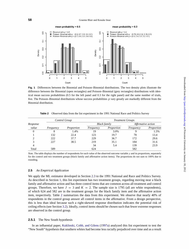
Although the two distributions have identical means, the Poisson–Binomial distribution is differentfrom the Binomial distribution. Figure1 illustrates the difference between the two distributions with fivetrials and selected mean success probabilities (0.5 for the left panel and 0.3 for the right panel). The figureshows that although the means are identical, these distributions can be quite different especially when thevariation of success probabilities is large (the density represented by dark grey rectangles). In general,the variance of the Poisson–Binomial distribution is no greater than that of the Binomial distribution.17
Given this discussion, the exact likelihood function for the modified design should be based on thePoisson–Binomial distribution. In Appendix4, we derive this exact likelihood function and develop anEM algorithm to estimate model parameters.
16In the first step, we fit each model defined in equation (17) to the control group using NLS. This step yields a consistent estimate ofθ j for j = 1, . . . , J. Denote this estimate byθ j . In the second step, we substituteθ j into the model defined in equation (16) and fit
the model for the sensitive itemg(x, δ) to the treatment group using NLS with the adjusted response variableYi −∑J
j =1 π j (x, θ j ).Thisstep yields a consistent estimate ofδ.
17Formally, we have∑J+1
j =1 π j (Xi , θ j )(1 − π j (Xi , θ j )) 6 (J + 1)π(Xi , θ)(1 − π(Xi , θ)). Ehm(1991) shows that the Poisson–Binomial distribution is well approximated by the Binomial distribution if and only if the variance of success probabilities, i.e.,∑J+1
j =1 (π j (Xi , θ j )− π(Xi , θ))2/(J + 1), is small relative toπ(Xi , θ)(1 − π(Xi , θ)).
at Princeton University on January 18, 2012
http://pan.oxfordjournals.org/D
ownloaded from
58 Graeme Blair and Kosuke Imai
Fig. 1 Differences between the Binomial and Poisson–Binomial distributions. The two density plots illustrate thedifference between the Binomial (open rectangles) and Poisson–Binomial (grey rectangles) distributions with iden-tical mean success probabilities (0.5 for the left panel and 0.3 for the right panel) and the same number of trials,five. The Poisson–Binomial distributions whose success probabilitiesp vary greatly are markedly different from theBinomial distribution.
Table 2 Observed data from the list experiment in the 1991 National Race and Politics Survey
Control Group Treatment GroupsResponse Black family Affirmativeaction
value Frequency Proportion Frequency Proportion Frequency Proportion0 8 1.4% 19 3.0% 9 1.5%1 132 22.4 123 19.7 78 13.42 222 37.7 229 36.7 172 29.63 227 38.5 219 35.1 184 31.64 34 5.4 139 23.9
Total 589 624 582
Note.The table displays the number of respondents for each value of the observed outcome variabley and its proportions, separatelyfor the control and two treatment groups (black family and affirmative action items). The proportions do not sum to 100% due torounding.
2.5 An Empirical Application
We apply the ML estimator developed in Section2.3 to the 1991 National and Race and Politics Survey.As described in Section1, this list experiment has two treatment groups, regarding moving near a blackfamily and affirmative action and has three control items that are common across all treatment and controlgroups. Therefore, we haveJ = 3 and K = 2. The sample size is 1795 (all are white respondents),of which 624 and 582 are in the treatment groups for the black family item and the affirmative actionitem, respectively. Table2 summarizes the data from this experiment. We observe that nearly 40% ofrespondents in the control group answer all control items in the affirmative. From a design perspective,this is less than ideal because such a right-skewed response distribution indicates the potential risk ofceiling effects (see Section3.2). Ideally, control items should be chosen such that fewer extreme responsesare observed in the control group.
2.5.1 The New South hypothesis
In an influential paper,Kuklinski, Cobb, and Gilens(1997a) analyzed this list experiment to test the“New South” hypothesis that southern whites had become less racially prejudiced over time and as a result
at Princeton University on January 18, 2012
http://pan.oxfordjournals.org/D
ownloaded from

StatisticalAnalysis of List Experiments 59
Table 3 Estimatedcoefficients from the combined logistic regression model where the outcome variables arewhether or not “A Black Family Moving Next Door to You” and whether or not “Black Leaders Asking the
Government for Affirmative Action” will make (white) respondentsangry
Sensitiveitems Control items
Black family Affirmativeaction
Variables Est. SE Est. SE Est. SE
Intercept −7.575 1.539 −5.270 1.268 1.389 0.143Male 1.200 0.569 0.538 0.435 −0.325 0.076College −0.259 0.496 −0.552 0.399 −0.533 0.074Age 0.852 0.220 0.579 0.147 0.006 0.028South 4.751 1.850 5.660 2.429 −0.685 0.297South× age −0.643 0.347 −0.833 0.418 0.093 0.061Control itemsYi (0) 0.267 0.252 0.991 0.264
Note. The key variables of interest are South, which indicates whether or not a respondent lives in one of the Southern states, and itsinteraction with the age variable.
thelevel of their racial prejudice had become no higher than that of non-southern whites. The authors usedthe simple difference-in-means estimator and estimated the difference in the proportions of those whoanswer each sensitive item in the affirmative between southern and non-southern whites. They find thatsouthern whites are substantially more racially prejudiced than non-southern whites with respect to bothsensitive items. However, as acknowledged by the authors (pp. 334–335), in the absence of multivariateregression techniques at that time, they were unable to adjust for differences in individual characteristicsbetween southern and non-southern whites, which could explain the difference in the degree of racialprejudice they found.
Furthermore, at the core of the New South hypothesis is a theory of generational change. AsKuklinski,Cobb, and Gilens(1997a) put it, “Young white southerners look more like their non-southern counterpartsthan their parents did; and the older generations themselves have become more willing to acknowledge therights of black people” (p. 325). Due to the lack of multivariate regression methods for list experiments,however, the original analysis of this generational change dichotomized the age variable in a particularmanner and compared the mean level of prejudice among white southerners born before 1960 to thoseborn after 1960, finding that the estimated proportion of those southern whites who are angry declinedfrom 47% to 35%. Clearly, a better approach is to treat age as a multivalued variable rather than a binaryvariable.
We apply our proposed multivariate regression methodology and improve the original analysis at leastin three ways. First, we take into account potentially confounding demographic differences betweensouthern and non-southern whites. We adjust for age, education (whether respondents attended college),and the gender of survey respondents. Second, we analyze three groups (two treatment and one controlgroups) together to take advantage of the fact that the same set of control items were asked in all groups,thereby improving statistical efficiency. Finally, we examine the generational changes among southernand non-southern whites by utilizing the interaction variable in regression rather than dichotomizing theage variable.
Table3 presents the estimated coefficients and their standard errors from the fitted binomial logisticregression model where we analyze the two treatment groups and one control group simultaneously. Weinclude the interaction term between the age and south variables in order to examine possibly differentgenerational changes among southern and non-southern whites.18 We find that both the age and southvariables play a significant role in explaining the variation in answering the sensitive item affirmatively. Inaddition, there appear to be different patterns in generational changes between southern and non-southernwhites. These findings are obtained while adjusting for gender and education level.
18Thelikelihood ratio test, comparing the model presented in this paper and the expanded model with the square of the age variableand its interaction with the South variable, fails to reject the null hypothesis of no difference between the two models, withp valueof 0.840.
at Princeton University on January 18, 2012
http://pan.oxfordjournals.org/D
ownloaded from
60 Graeme Blair and Kosuke Imai
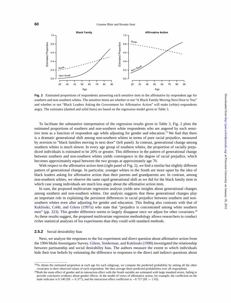
Fig. 2 Estimated proportions of respondents answering each sensitive item in the affirmative by respondent age forsouthern and non-southern whites. The sensitive items are whether or not “A Black Family Moving Next Door to You”and whether or not “Black Leaders Asking the Government for Affirmative Action” will make (white) respondentsangry. The estimates (dashed and solid lines) are based on the regression model given in Table3.
To facilitate the substantive interpretation of the regression results given in Table3, Fig. 2 plots theestimated proportions of southern and non-southern white respondents who are angered by each sensi-tive item as a function of respondent age while adjusting for gender and education.19 We find that thereis a dramatic generational shift among non-southern whites in terms of pure racial prejudice, measuredby aversion to “black families moving in next door” (left panel). In contrast, generational change amongsouthern whites is much slower. In every age group of southern whites, the proportion of racially preju-diced individuals is estimated to be 20% or greater. This difference in the pattern of generational changebetween southern and non-southern whites yields convergence in the degree of racial prejudice, whichbecomes approximately equal between the two groups at approximately age 70.
With respect to the affirmative action item (right panel of Fig.2), we find a similar but slightly differentpattern of generational change. In particular, younger whites in the South are more upset by the idea ofblack leaders asking for affirmative action than their parents and grandparents are. In contrast, amongnon-southern whites, we observe the same rapid generational shift as we did for the black family item inwhich case young individuals are much less angry about the affirmative action item.
In sum, the proposed multivariate regression analysis yields new insights about generational changesamong southern and non-southern whites. Our analysis suggests that these generational changes playan important role in explaining the persistent differences in racial prejudice between southern and non-southern whites even after adjusting for gender and education. This finding also contrasts with that ofKuklinski, Cobb, and Gilens(1997a) who state that “prejudice is concentrated among white southernmen” (pp. 323). This gender difference seems to largely disappear once we adjust for other covariates.20
As these results suggest, the proposed multivariate regression methodology allows researchers to conductricher statistical analyses of list experiments than they could with standard methods.
2.5.2 Social desirability bias
Next, we analyze the responses to the list experiment and direct question about affirmative action fromthe 1994 Multi-Investigator Survey.Gilens, Sniderman, and Kuklinski(1998) investigated the relationshipbetween partisanship and social desirability bias. The authors measure the extent to which individualshide their true beliefs by estimating the difference in responses to the direct and indirect questions about
19To obtain the estimated proportion at each age for each subgroup, we compute the predicted probability by setting all the othercovariates to their observed values of each respondent. We then average these predicted probabilities over all respondents.
20Both the main effect of gender and its interaction effect with the South variable are estimated with large standard errors, failing toprovide conclusive evidence about gender effects. In the model of views of affirmative action, for example, the coefficient on themale indicator is 0.140 (SE= 0.377), and the interaction effect coefficient is−0.757 (SE= 1.03).
at Princeton University on January 18, 2012
http://pan.oxfordjournals.org/D
ownloaded from
Statistical Analysis of List Experiments 61
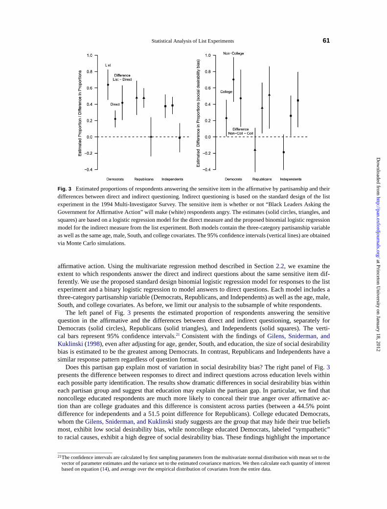
Fig. 3 Estimated proportions of respondents answering the sensitive item in the affirmative by partisanship and theirdifferences between direct and indirect questioning. Indirect questioning is based on the standard design of the listexperiment in the 1994 Multi-Investigator Survey. The sensitive item is whether or not “Black Leaders Asking theGovernment for Affirmative Action” will make (white) respondents angry. The estimates (solid circles, triangles, andsquares) are based on a logistic regression model for the direct measure and the proposed binomial logistic regressionmodel for the indirect measure from the list experiment. Both models contain the three-category partisanship variableas well as the same age, male, South, and college covariates. The 95% confidence intervals (vertical lines) are obtainedvia Monte Carlo simulations.
affirmative action. Using the multivariate regression method described in Section2.2, we examine theextent to which respondents answer the direct and indirect questions about the same sensitive item dif-ferently. We use the proposed standard design binomial logistic regression model for responses to the listexperiment and a binary logistic regression to model answers to direct questions. Each model includes athree-category partisanship variable (Democrats, Republicans, and Independents) as well as the age, male,South, and college covariates. As before, we limit our analysis to the subsample of white respondents.
The left panel of Fig.3 presents the estimated proportion of respondents answering the sensitivequestion in the affirmative and the differences between direct and indirect questioning, separately forDemocrats (solid circles), Republicans (solid triangles), and Independents (solid squares). The verti-cal bars represent 95% confidence intervals.21 Consistent with the findings ofGilens, Sniderman, andKuklinski (1998), even after adjusting for age, gender, South, and education, the size of social desirabilitybias is estimated to be the greatest among Democrats. In contrast, Republicans and Independents have asimilar response pattern regardless of question format.
Does this partisan gap explain most of variation in social desirability bias? The right panel of Fig.3presents the difference between responses to direct and indirect questions across education levels withineach possible party identification. The results show dramatic differences in social desirability bias withineach partisan group and suggest that education may explain the partisan gap. In particular, we find thatnoncollege educated respondents are much more likely to conceal their true anger over affirmative ac-tion than are college graduates and this difference is consistent across parties (between a 44.5% pointdifference for independents and a 51.5 point difference for Republicans). College educated Democrats,whom theGilens, Sniderman, and Kuklinskistudy suggests are the group that may hide their true beliefsmost, exhibit low social desirability bias, while noncollege educated Democrats, labeled “sympathetic”to racial causes, exhibit a high degree of social desirability bias. These findings highlight the importance
21The confidence intervals are calculated by first sampling parameters from the multivariate normal distribution with mean set to thevector of parameter estimates and the variance set to the estimated covariance matrices. We then calculate each quantity of interestbased on equation (14), and average over the empirical distribution of covariates from the entire data.
at Princeton University on January 18, 2012
http://pan.oxfordjournals.org/D
ownloaded from

62 GraemeBlair and Kosuke Imai
of adjusting for additional covariates, which is made possible by the proposed multivariate regressionanalysis.
Finally, we emphasize that this measure of social desirability bias relies on Assumptions1 and2. Ifthese assumptions are violated, then the estimates based on list experiments are invalid and hence thedifference between responses to direct questioning and list experiments no longer represent the degree ofsocial desirability bias. For example, it is possible that college educated Democrats are more likely to lieunder the list experiment than noncollege educated Democrats and that this may explain the differencewe observe. We address this issue in Section3 by developing statistical methods to detect and correctviolations of the assumptions.
2.6 A Simulation Study
We now compare the performance of three estimators for the modified design: LISTIT (Corstange 2009)as well as the proposed NLS and ML estimators. Our Monte Carlo study is based upon the simulationsettings reported inCorstange(2009). We sample a single covariate from the uniform distribution and usethe logistic regression model for the sensitive item where the true values of the intercept and the coefficientare set to 0 and 1, respectively. We vary the sample size from 500 to 1500 and consider two differentnumbers of control items, three and four. We begin by replicating one of the simulation scenarios used inCorstange(2009), where the success probability is assumed to be identical across all three control items.Thus, the true values of coefficients in the logistic models are all set to one. In the other three scenarios, werelax the assumption of equal probabilities. FollowingCorstange, we choose the true values of coefficientssuch that the probabilities for the control items are equal to
(12,
14,
34
)(threecontrol items with unequal
symmetric probabilities),(1
5,25,
35,
45
)(four control items with unequal, symmetric probabilities), and
(16,
36,
46,
46
)(four control items with unequal, skewed probabilities).
Figure4 summarizes the results based on 10,000 independent Monte Carlo draws for each scenario.The four columns represent different simulation settings and the three rows report bias, root mean squarederror (RMSE), and the coverage of 90% confidence intervals. As expected, across all four scenarios andin terms of all three criteria considered here, the ML estimator (open circles) exhibits the best statisticalproperties, while the NLS estimator (solid circles) outperforms the LISTIT estimator (open diamonds).The differences are larger when the sample size is smaller. When the sample size is as large as 1,500,the performance of all three estimators is similar in terms of bias and RMSE. Given that both the NLSand LISTIT estimators model the conditional means correctly, the differences can be attributed to the factthat the ML estimator incorporates the knowledge of response distribution. In addition, a large bias of theLISTIT estimator in small samples may come from the failure of the Newton-Raphson-type optimizationused to maximize the complex likelihood function. This may explain why the LISTIT estimator doesnot do well even in the case of equal probabilities. In contrast, our EM algorithm yields more reliablecomputation of the ML estimator.
In sum, this simulation study suggests that our proposed estimators for the modified design can outper-form the existing estimator in terms of bias, RMSE, and the coverage probability of confidence intervalsespecially when the sample size is small.
3 Detectingand Correcting Failures of List Experiments
The validity of statistical analyses of list experiments, including those discussed in previous studies andthose based on the methods proposed above, depends critically upon the two assumptions described inSection2.1: the assumption of no design effect (Assumption1) and that of no liars (Assumption2).When analyzing list experiments, any careful empirical researcher should try to detect violations of theseassumptions and make appropriate adjustments for them whenever possible.
In this section, we develop new statistical methods to detect and adjust for certain types of list experi-ment failures. We first propose a statistical test for detectingdesign effects, in which the inclusion of asensitive item changes responses to control items. We then extend the identification analysis and likelihoodinference framework described in Section2.1to address potential violations of another key assumption –respondents give truthful answers to the sensitive item. In particular, we modelceiling and floor effects,which may arise under certain circumstances in which respondents suppress their truthful answers to thesensitive item despite the anonymity protections offered by list experiments.
at Princeton University on January 18, 2012
http://pan.oxfordjournals.org/D
ownloaded from

Statistical Analysis of List Experiments 63
Fig. 4 Monte Carlo evaluation of the three estimators, LISTIT (Corstange 2009), NLS, and ML. Four simulationscenarios are constructed. The left most column is identical to a simulation setting ofCorstange(2009) with threecontrol items whose probability distributions are identical. The other columns relax the assumption of equal probabil-ities with different numbers of control items. Bias (first row), root mean squared error (second row), and the coverageof 90% confidence intervals (third row) for the estimated coefficient are reported under each scenario. The samplesize varies from 500 to 1500. In all cases, the ML estimator (open circles) has the best performance while the NLSestimator (solid circles) has better statistical properties than the LISTIT estimator (open diamonds). The differencesare larger when the sample size is smaller.
3.1 A Statistical Test for Detecting Design Effects
First, we develop a statistical test for detecting potential violations of Assumption1 by considering thescenario in which the inclusion of a sensitive item affects some respondents’ answers to control items.Such a design effect may arise if respondents evaluate control items relative to the sensitive item, yieldingdifferent propensities to answer control items affirmatively across the treatment and control conditions.We define the average design effect as the difference in average response between treatment and controlconditions,
Δ= E(Yi (0) | Ti = 1)− E(Yi (0) | Ti = 0). (18)
The goal of the statistical test we propose below is to detect the existence of such a design effect.
3.1.1 Setup
We first consider the standard design described in Section2.1. Our statistical test exploits the factthat under the standard assumptions all of the proportions of respondent types, i.e.,πyt ’s, are identified
at Princeton University on January 18, 2012
http://pan.oxfordjournals.org/D
ownloaded from

64 GraemeBlair and Kosuke Imai
(seeSection2.1). If at least one of these proportions is negative, the assumption of no design effect isnecessarily violated (see alsoGlynn 2010). Note that the violation of Assumption2 alone does not lead tonegative proportions of these types while it may make it difficult to identify certain design effects. Thus,the statistical test described below attempts to detect violation of Assumption1.
Formally, using equations (2) and (3), we can express the null hypothesis as follows:
H0 :
{Pr(Yi 6 y|Ti = 0)> Pr(Yi 6 y|Ti = 1) for all y = 0, . . . , J − 1 and
Pr(Yi 6 y|Ti = 1) > Pr(Yi 6 y − 1|Ti = 0) for all y = 1, . . . , J.(19)
Note that some values ofy are excluded because in those cases the inequalities are guaranteed to be satis-fied. An equivalent expression of the null hypothesis isπyt > 0 for all y andt . The alternative hypothesisis that there existsat leastone value ofy that does not satisfy the inequalities given in equation (19).
Given this setup, our proposed test reduces to a statistical test of two first-order stochastic dominancerelationships. Intuitively, if the assumption of no design effect is satisfied, the addition of the sensi-tive item to the control list makes the response variable of the treatment group larger than the controlresponse (the first line of equation (19)) but at most by one item (the second line of equation (19)). If theestimates ofπyt ’s are negative and unusually large, we may suspect that the null hypothesis of no designeffect is false.
The form of the null hypothesis suggests that in some situations the detection of design effects is dif-ficult. For example, when the probability of an affirmative answer to the sensitive item is around 50%,design effects may not manifest themselves clearly unless the probability of answering affirmatively tocontrol items differs markedly under the treatment and control conditions (i.e., the design effect is large).Alternatively, when the probability of answering affirmatively to the sensitive item is either small (large)and the design effectΔ is negative (positive), then the power of the statistical test is greater. This asymme-try offers some implications for design of list experiments. In particular, when only few (a large numberof) people hold a sensitive viewpoint, researchers may be able to choose control items such that the likelydirection of design effect, if it exists, is going to be negative (positive) so that the power of the proposedtest is greater.
3.1.2 The proposed testing procedure
Clearly, if all the estimated proportionsπyt arenonnegative, then we fail to reject the null hypothesis.If some of the estimated proportions are negative, however, then the critical question is whether suchnegative values have arisen by chance. The basic idea of our proposed statistical testing procedure is tofirst conduct a separate hypothesis test for each of the two stochastic dominance relationships given inequation (19) and then combine the results using the Bonferroni correction.22 That is, we compute twop values based on the two separate statistical tests of stochastic dominance relationships and then rejectthe null hypothesis if and only if the minimum of these twop values is less thanα/2, whereα is thedesired size of the test chosen by researchers, for example,α = 0.05. Note that the threshold is adjusteddownward, which corrects for false positives due to multiple testing. This Bonferroni correction results insome loss of statistical power but directly testing the entire null hypothesis is difficult because the leastfavorable value ofπ under the null hypothesis is not readily available (seeWolak 1991).
To test each stochastic dominance relationship, we use the likelihood ratio test based on the asymptoticmultivariate normal approximation (seeKudo 1963; Perlman 1969). The test statistic is given by
λt = minπt(πt − πt )
>Σ−1t (πt − πt ) subjectto πt > 0 (20)
for t = 0,1, whereπt is the J dimensional stacked vector ofπyt ’s andΣt is a consistent estimate ofthe covariance matrix ofπt . It has been shown that thep value of the hypothesis test based onλt canbe computed based upon the mixture of chi-squared distributions. Finally, to improve the power of the
22Whentest statistics are either independent or positively dependent, a procedure that uniformly improves the Bonferroni correctionhas been developed (see, e.g.,Holland and Copenhaver 1987, Section 3). However, in our case, the two test statistics are negativelycorrelated, implying that improvement over the Bonferroni correction may be difficult.
at Princeton University on January 18, 2012
http://pan.oxfordjournals.org/D
ownloaded from

StatisticalAnalysis of List Experiments 65
proposedtest, we employ the generalized moment selection (GMS) procedure proposed byAndrews andSoares(2010). The GMS procedure can improve the power of the test in some situations because inpractice many of the moment inequalities,πyt > 0, are unlikely to be binding and hence can be ignored.The technical details of the test including the expression ofΣ is given in Appendix4.
3.1.3 Applications to other designs
The statistical test proposed above can be applied to the other designs considered in Section2. First,consider the design with multiple sensitive items. If there existK sensitive items, for each sensitive itemwe can form the null hypothesis of no design effect given in equation (19) and conduct the proposedstatistical test.23
Similarly, the proposed test can be applied to the design with the direct questioning of control items inthe control group. Under this design, the careful examination of possible design effect may be especiallyimportant because the control group is presented with each item rather than a list of items. Based on thetwo list experiments about racial prejudice in the United States, for example,Flavin and Keane(2009)find that respondents’ answers to control items differ depending on whether they are asked directly. Theapplication of the proposed statistical test under this design is straightforward. Before applying the test,researchers must aggregate all the separate answers to control items for each respondent in the controlgroup, that is,Yi (0) =
∑Jj =1 Zi (0). Once this is done, our proposed statistical test can be applied to this
alternative design in the exactly same manner as under the standard design.
3.1.4 Limitations
Finally, we briefly discuss the limitations of the proposed hypothesis test. First, it is important toemphasize that, as is the case in general for any statistical hypothesis test, the failure to reject the nullhypothesis of no design effect does not necessarily imply that Assumption1 is validated. In particular,researchers may fail to reject the null hypothesis due to a lack of statistical power. For example, certainviolations of Assumption2 may mask the presence of design effects. Correction for multiple testing alsoreduces the power of statistical tests for design effects. After describing the proposed statistical test, weconduct a Monte Carlo simulation study to assess its statistical power. Second, the proposed test mayfail to detect design effects if positive design effects from some respondents are canceled out by negativedesign effects from others. To address this problem, one may apply the proposed test to different subsets ofthe data but such an approach often lacks statistical power and also faces the problem of multiple testing.
These limitations point to the simple and general fact that the failure to reject the null hypothesis of nodesign effect should not be taken as evidence to support the null hypothesis (although the rejection of thenull hypothesis certainly constitutes evidence against it).
3.2 Adjustingfor Ceiling and Floor Effects
Even if we assume that design effects do not exist (Assumption1), we may wish to address the possibilitythat some respondents in the treatment group lie about the sensitive item, which would violate Assump-tion 2. Below, we consider two scenarios in which this second assumption is violated. The first is theproblem of a “ceiling effect,” which is caused by the fact that privacy is not protected for those respon-dents in the treatment group whose true preferences are affirmative for all the sensitive and control items.Here, we entertain the possibility that some of these respondents would lie and give an answerYi = JratherthanYi = J + 1 in order to conceal their true affirmative preference for the sensitive item.
We also investigate the possibility of a “floor effect” in which some of the respondents whose truthfulanswer is affirmative only for the sensitive item (and thus negative for all control items) giveYi = 0 asan answer instead of the truthfulYi = 1. This may occur when the control items are expected to generatemany negative answers. In such a situation, the respondents in the treatment group whose truthful answeris affirmative only for the sensitive item may fear that their true preference for the sensitive item would be
23If desired, a procedure can be derived to further account for multiple testing acrossK sensitive items (e.g., by controlling the falsediscovery rate), but the development of such a procedure is beyond the scope of this paper.
at Princeton University on January 18, 2012
http://pan.oxfordjournals.org/D
ownloaded from

66 GraemeBlair and Kosuke Imai
Table 4 An example illustrating ceiling and floor effects under the standard design with three controlitems
Response Treatment group Control groupYi (Ti = 1) (Ti = 0)
4 (3, 1)3 (2, 1) (3, 0) (3, 1)† (3, 1) (3, 0)2 (1, 1) (2, 0) (2, 1) (2, 0)1 (0, 1) (1, 0) (1, 1) (1, 0)0 (0, 0) (0, 1)† (0, 1) (0,0)
Note. The table shows how each respondent type, characterized by(Yi (0), Z∗i,J+1), corresponds to the observed cell defined by
(Yi , Ti ), whereYi (0) representsthe total number of affirmative answers forJ control items andZ∗i,J+1 denotesthe truthful prefer-
ence for the sensitive item. The symbol † represents liars who are affected by ceiling and floor effects.
revealed by givingYi = 1 as their answer. For the reminder of this section, we assume that the number ofcontrol items is no less than three (J > 3) to focus on realistic situations.
3.2.1 Setup
What are the consequences of such violations of Assumption2? Table4 illustrates ceiling and flooreffects when there are three control items. The difference between this table and Table1 is the presence ofceiling and floor effects. Among those in the treatment group who give the answerYi = 3, for example,there exist some respondents whose truthful answer isYi = 4. Similarly, some of the respondents in thetreatment group who give the answerYi = 0 are lying, since their truthful answer is affirmative for thesensitive item. In the table, the types of these respondents are marked with the symbol †.
Intuitively, the presence of such ceiling and floor effects would lead to the underestimation of thepopulation proportion of those who would answer affirmatively for the sensitive item. This is becauseboth types of lies lower the observed mean response of the treatment group. How large can this bias be?To derive the magnitude of bias, we begin by defining the conditional probability of lying under these twoscenarios as,
q ≡ Pr(Yi (1)= J|Yi (0)= J, Z∗i,J+1 = 1), (21)
q ≡ Pr(Yi (1)= 0|Yi (0)= 0, Z∗i,J+1 = 1). (22)
In words,q represents the population proportion of liars who give the answerYi = J if assigned to thetreatment condition, among the respondents whose truthful answer is affirmative for both sensitive andcontrol items. Similarly,q denotesthe population proportion of liars who reportYi = 0 if assigned tothe treatment condition, among the respondents whose truthful answer is affirmative only for the sensitiveitem. Whenq = 0 (q = 0), the standard assumption holds and the ceiling effects (the floor effects)are zero.
Given these definitions, Table4 shows that the respondents in the treatment group who answerYi =J + 1 consist of the(1 − q) proportion of the respondent type(Yi (0), Z∗
i,J+1) = (J, 1), whereas thosein the treatment group whose answer isYi = J area mixture of three types:(J − 1,1), (J, 0), and theqproportion of the type(J, 1). Similarly, the respondents in the treatment group whose answer isYi = 0form a mixture of two types,(0,0) and the proportionq of the type(0,1), whereas those in the treatmentgroup who give the answerYi = 1 also consist of two types:(1,0) and the proportion(1 − q) of thetype(0,1).
3.2.2 Modeling ceiling and floor effects
One approach to the potential existence of ceiling and/or floor effects is to derive the sharp boundson the true population proportion for the sensitive item (Manski 2007). Such an approach characterizeswhat can be learned about responses to the sensitive item from the observed data alone without makingadditional assumptions. In Appendix4, we show that the existence of ceiling and/or floor effects leadsto underestimation of the true population for the sensitive item. However, this approach cannot easily
at Princeton University on January 18, 2012
http://pan.oxfordjournals.org/D
ownloaded from

StatisticalAnalysis of List Experiments 67
incorporatevarious types of covariates. As a result, the direction and magnitude of bias are difficult toascertain for estimating the effects of these covariates on the probability of answering the sensitive itemaffirmatively.
To overcome these limitations, we take an alternative strategy of directly modeling certain ceilingand floor effects at the cost of making an additional assumption. This strategy will allow researchersto estimate the population proportion of respondents responding affirmatively to the sensitive item aswell as the relationship between covariates and the probability of answering in the affirmative. Below,we present one way to model dishonest responses in the form of ceiling and floor effects within thelikelihood framework described in Section2.1. The proposed methodology, therefore, enables inferencesabout responses to the sensitive item and their association with covariates, while correcting for certainviolations of Assumption2.
In the absence of ceiling and floor effects,πyz is just identified, meaning that the identification of thisquantity requires the use of all information contained in the data.24 One implication of this fact is thatto model ceiling and floor effects we must introduce at least two additional constraints because we nowhave to identify two additional unknown quantities,q andq. Our proposed assumption is that respondents’truthful answer for the sensitive item is independent of their answers for control items conditional upon thepretreatment covariatesXi . Such an assumption may be plausible if, for example, the control items are notsubstantively related to the sensitive item. Moreover, researchers may be able to increase the plausibilityof this assumption by collecting relevant covariates that can predict respondents’ answers so that what isleft unexplained for each item can be thought of as an idiosyncratic error term. We emphasize that thisassumption may not be plausible in certain applications and must be made with great care. If liars decidetheir truthful responses to sensitive items based on their answers to control items, for example, then thisassumption will be violated.
Formally, the assumption can be written as
Pr(Yi (0)= y|Z∗i,J+1 = 1,Xi = x)= Pr(Yi (0)= y|Z∗
i,J+1 = 0,Xi = x) (23)
for all y = 0,1, . . . , J given anyx. It can be shown thatπyz is identified under this additional assumptioneven when ceiling and floor effects exist.25 Under this assumption, we define the model for the controlitem ash(y; x, ψ) = Pr(Yi (0) = y|Xi = x) underthe conditional independence assumption given inequation (23). We then modelq andq usingcovariates as
q(x, φ)= Pr(Yi (1)= J|Yi (0)= J, Z∗i,J+1 = 1,Xi = x), (24)
q(x, κ)= Pr(Yi (1)= 0|Yi (0)= 0, Z∗i,J+1 = 1,Xi = x). (25)
In Supplementary Materials Section 3, we derive the likelihood function based on this approach and de-velop an EM algorithm to estimate model parameters. While the setup is general, in practice we mayuse binomial logistic regression models for each component,g(x, δ), h(y; x, ψ), q(x, φ), andq(x, κ).In some applications, including the racial prejudice example analyzed below, we find that complete sep-aration of covariates occurs in logistic regression models when adding the models for ceiling and flooreffects. In such situations, weakly informative priors can be added to the models for ceiling/floor effectsby following the recommendations ofGelman et al.(2008) and calculating the uncertainty estimates basedon this pseudoposterior distribution.
24To see why this is the case, note that there exist(2× (J +1)) types of respondents. Since the population proportions of these typeshave to sum to unity, there are a total of(2J +1) unknowns. Now, for these unknown quantities, the data from the treatment groupprovide(J +1) independent linear constraints and the data from the control group provideJ independent linear constraints (againnoting the fact that within each group the observed proportions of each response have to sum up to unity). Since the number oflinearly independent constraints match exactly with the number of unknowns, it follows thatπyz is just identified.
25Specifically, equation (23) implies the following nonlinear constraint,∑J
j ′=0 π j ′1 =π j 1
π j 1+π j 0for each j = 0, . . . , J. Therefore,
there exist a total(3J +2) constraints including(2J +1) constraints that are already implied by the data generating process. Whenthe ceiling and floor effects are present, there are(2J + 3) unknowns and therefore identification is possible.
at Princeton University on January 18, 2012
http://pan.oxfordjournals.org/D
ownloaded from

68 GraemeBlair and Kosuke Imai
3.2.3 Quantitiesof interest
When modeling ceiling and floor effects, we may be interested in the conditional probability of lyingunder two scenarios. First, the population proportion of liars among those who would affirmatively answerboth sensitive and control items, as defined in equation (21), is given by,
q =∫
q(Xi ;ψ)dP(Xi |Yi (0)= J, Z∗i,J+1 = 1)
=
∫q(Xi ;ψ)h(J; Xi , φ)g(Xi , δ)dP(Xi )∫
h(J, ; Xi , φ)g(Xi , δ)dP(Xi )≈
∑ni =1 q(Xi ;ψ)h(J; Xi , φ)g(Xi , δ)∑n
i =1 h(J, ; Xi , φ)g(Xi , δ), (26)
where the second equality follows from Bayes’ rule and the distribution ofXi is approximated by itsempirical distribution. In addition, researchers may be interested in the population proportions of theseliars. In the case of ceiling effects, this quantity can be estimated as
Pr(Zi,J+1(1)= 0, Z∗i,J+1 = 1,Yi (0)= J)≈
1
n
n∑
i =1
q(Xi ;ψ)h(J; Xi , φ)g(Xi , δ). (27)
Similarly, the population proportion of liars among those who would negatively answer all control itemsand answer affirmatively about the sensitive item, that is,q definedin equation (22), is approximated by
q ≈
∑ni =1 q(Xi ;ψ)h(0; Xi , φ)g(Xi , δ)∑n
i =1 h(0; Xi , φ)g(Xi , δ). (28)
The population proportion of these liars can be estimated as follows:
Pr(Zi,J+1(1)= 0, Z∗i,J+1 = 1,Yi (0)= 0)≈
1
n
n∑
i =1
q(Xi ;ψ)h(0; Xi , φ)g(Xi , δ). (29)
3.3 Adjustingfor Design Effects
The modeling strategy described above can be also used to adjust for certain design effects. As a generalexample, consider a situation where there is a negative design effect such that adding the sensitive itemmay reduce the answer of some respondents by at most one item. This scenario is summarized in Table5in the same manner as Table4. Under the assumption of independence between responses to sensitiveand control items, we have two free parameters. Thus, we may model the probability of being affectedby this negative design effect separately for those whose answer to the sensitive item is affirmative andthose whose answer is not affirmative, that is,r0(x) = Pr(Yi = j − 1|Yi (0) = j, Z∗
i,J+1 = 0,Xi = x)andr1(x) = Pr(Yi = j − 1|Yi (0) = j − 1, Z∗
i,J+1 = 1,Xi = x), respectively. Given this setup, theML estimation can be accomplished in a manner similar to the way described in Supplementary MaterialsSection 3.
Table 5 An example illustrating a particular negative design effect under the standard design with threecontrolitems
Response Treatment group Control groupYi (Ti = 1) (Ti = 0)4 (3,1)3 (2,1) (3,0) (3,1)† (3,1)(3,0)2 (1,1) (2,0) (2,1)† (3,0)† (2,1)(2,0)1 (0,1) (1,0) (1,1)† (2,0)† (1,1)(1,0)0 (0,0) (1,0)† (0,1) (0,0)
Note. The table shows how each respondent type, characterized by(Yi (0), Z∗i,J+1), corresponds to the observed cell defined by
(Yi , Ti ), whereYi (0) representsthe total number of affirmative answers forJ control items andZ∗i,J+1 denotesthe truthful pref-
erence for the sensitive item. The symbol † represents respondents who are affected by the negative design effect and underreporttheir total count by one.
at Princeton University on January 18, 2012
http://pan.oxfordjournals.org/D
ownloaded from
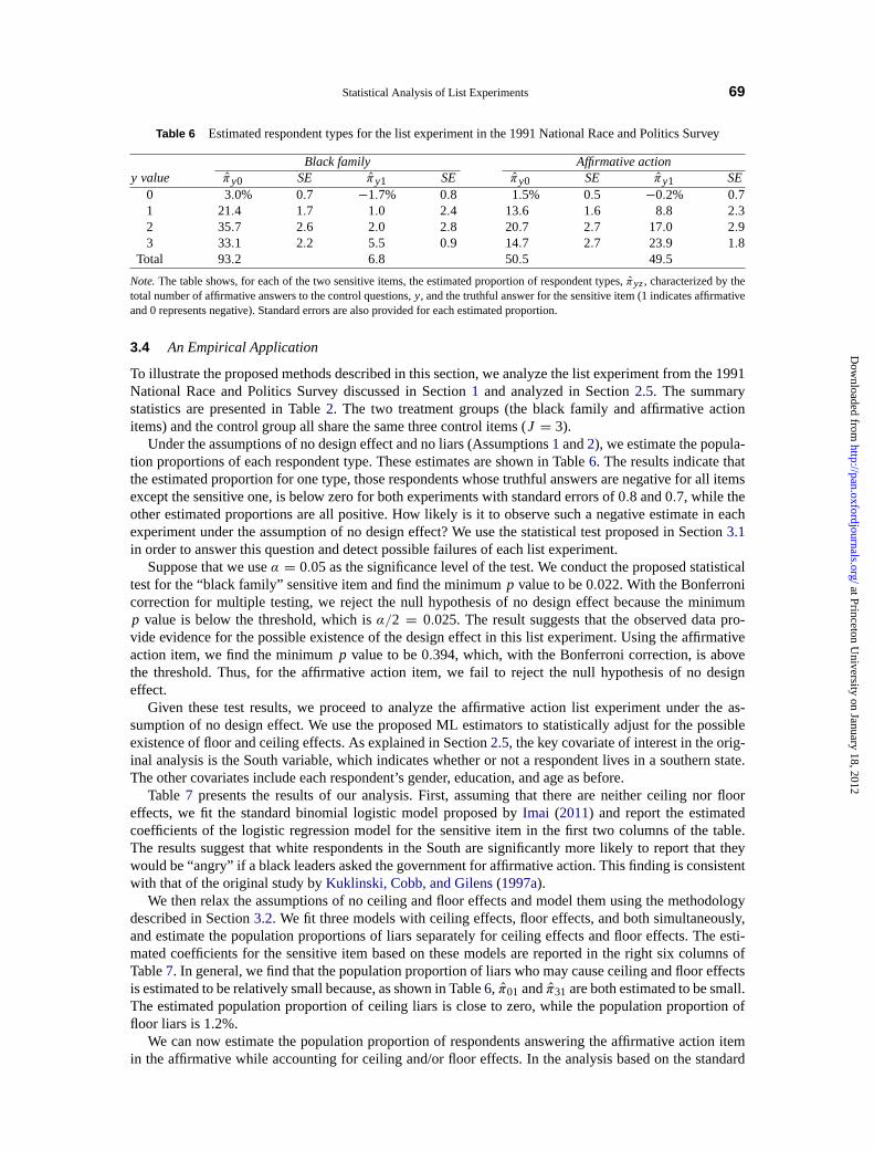
StatisticalAnalysis of List Experiments 69
Table 6 Estimatedrespondent types for the list experiment in the 1991 National Race and Politics Survey
Black family Affirmativeactiony value πy0 SE πy1 SE πy0 SE πy1 SE
0 3.0% 0.7 −1.7% 0.8 1.5% 0.5 −0.2% 0.71 21.4 1.7 1.0 2.4 13.6 1.6 8.8 2.32 35.7 2.6 2.0 2.8 20.7 2.7 17.0 2.93 33.1 2.2 5.5 0.9 14.7 2.7 23.9 1.8
Total 93.2 6.8 50.5 49.5
Note. The table shows, for each of the two sensitive items, the estimated proportion of respondent types,πyz, characterized by thetotal number of affirmative answers to the control questions,y, and the truthful answer for the sensitive item (1 indicates affirmativeand 0 represents negative). Standard errors are also provided for each estimated proportion.
3.4 AnEmpirical Application
To illustrate the proposed methods described in this section, we analyze the list experiment from the 1991National Race and Politics Survey discussed in Section1 and analyzed in Section2.5. The summarystatistics are presented in Table2. The two treatment groups (the black family and affirmative actionitems) and the control group all share the same three control items (J = 3).
Under the assumptions of no design effect and no liars (Assumptions1 and2), we estimate the popula-tion proportions of each respondent type. These estimates are shown in Table6. The results indicate thatthe estimated proportion for one type, those respondents whose truthful answers are negative for all itemsexcept the sensitive one, is below zero for both experiments with standard errors of 0.8 and 0.7, while theother estimated proportions are all positive. How likely is it to observe such a negative estimate in eachexperiment under the assumption of no design effect? We use the statistical test proposed in Section3.1in order to answer this question and detect possible failures of each list experiment.
Suppose that we useα = 0.05 as the significance level of the test. We conduct the proposed statisticaltest for the “black family” sensitive item and find the minimump value to be 0.022. With the Bonferronicorrection for multiple testing, we reject the null hypothesis of no design effect because the minimump value is below the threshold, which isα/2 = 0.025. The result suggests that the observed data pro-vide evidence for the possible existence of the design effect in this list experiment. Using the affirmativeaction item, we find the minimump value to be 0.394, which, with the Bonferroni correction, is abovethe threshold. Thus, for the affirmative action item, we fail to reject the null hypothesis of no designeffect.
Given these test results, we proceed to analyze the affirmative action list experiment under the as-sumption of no design effect. We use the proposed ML estimators to statistically adjust for the possibleexistence of floor and ceiling effects. As explained in Section2.5, the key covariate of interest in the orig-inal analysis is the South variable, which indicates whether or not a respondent lives in a southern state.The other covariates include each respondent’s gender, education, and age as before.
Table 7 presents the results of our analysis. First, assuming that there are neither ceiling nor flooreffects, we fit the standard binomial logistic model proposed byImai (2011) and report the estimatedcoefficients of the logistic regression model for the sensitive item in the first two columns of the table.The results suggest that white respondents in the South are significantly more likely to report that theywould be “angry” if a black leaders asked the government for affirmative action. This finding is consistentwith that of the original study byKuklinski, Cobb, and Gilens(1997a).
We then relax the assumptions of no ceiling and floor effects and model them using the methodologydescribed in Section3.2. We fit three models with ceiling effects, floor effects, and both simultaneously,and estimate the population proportions of liars separately for ceiling effects and floor effects. The esti-mated coefficients for the sensitive item based on these models are reported in the right six columns ofTable7. In general, we find that the population proportion of liars who may cause ceiling and floor effectsis estimated to be relatively small because, as shown in Table6, π01 andπ31 areboth estimated to be small.The estimated population proportion of ceiling liars is close to zero, while the population proportion offloor liars is 1.2%.
We can now estimate the population proportion of respondents answering the affirmative action itemin the affirmative while accounting for ceiling and/or floor effects. In the analysis based on the standard
at Princeton University on January 18, 2012
http://pan.oxfordjournals.org/D
ownloaded from

70 GraemeBlair and Kosuke Imai
Table 7 Estimatedcoefficients from the logistic regression models where the outcome variable is whether or not“Black Leaders Asking the Government for Affirmative Action” will make (white) respondentsangry
Without ceiling Both ceilingand floor effects Ceiling effects alone Floor effects alone and floor effects
Variables Est. SE Est. SE Est. SE Est. SEIntercept −1.299 0.556 −1.291 0.558 −1.251 0.501 −1.245 0.502Age 0.295 0.101 0.294 0.101 0.314 0.092 0.313 0.092College −0.343 0.336 −0.345 0.336 −0.605 0.298 −0.606 0.298Male 0.040 0.346 0.038 0.346 −0.088 0.300 −0.088 0.300South 1.177 0.480 1.175 0.480 0.682 0.335 0.681 0.335Proportion of liarsCeiling effects 0.0002 0.0017 0.0002 0.0016Floor effects 0.0115 0.0000 0.0115 0.0000
Note. The key coefficient of interest is the one for the variable South, which indicates whether or not a respondent lives in one ofthe southern states. The results in the left two columns are based on the standard Binomial logistic model ofImai (2011) (withoutceiling or floor effects), and the remaining columns report the results based on the models with ceiling effects, floor effects, and thenboth. The last two rows report the estimated population probability of lying separately for ceiling and floor effects.
binomial logistic model, we find that the difference between this proportion for respondents in the Southand for respondents in the non-South is 0.250 (SE= 0.095). After adjusting for ceiling and floor effects,the estimated difference in proportions is 0.146 (SE= 0.074), well within the margin of error. This findingis consistent with the result of a standard model selection procedure. Indeed, according to the Bayesianinformation criterion (BIC), the model without ceiling or floor effects is most preferred.26
In sum, the analysis reported here implies that the original conclusion ofKuklinski, Cobb, and Gilens(1997a)—the degree of racial prejudice is greater for southern whites than their non-southern counter-parts—is robust to the possible existence of ceiling and floor effects.
3.5 A Simulation Study
We conduct a Monte Carlo simulation study to explore the statistical power of the proposed test (with theGMS procedure) under various conditions. Figure5 presents the results of the simulation study. The datagenerating process is as follows: We independently sample the total number of affirmative answers to threecontrol itemsYi (0) from the binomial distribution with success probability equal to 0.25 (left column), 0.5(middle column), or 0.75 (right column). This means that the expected number of affirmative responsesto these control items is equal to 0.75, 1.5, and 2.25, respectively. We then sample the answer to thesensitive item, again independently, from the Bernoulli distribution with success probability equal to 0.1(top row), 0.25 (second row), 0.5 (middle row), 0.75 (fourth row), or 0.9 (bottom row). We also vary themagnitude of the average design effectΔ from −0.6 to 0.6 (horizontal axis). Finally, we consider threedifferent realistic sample sizes, 500, 1000, and 1500. For all the simulations we conduct, the size of thetreatment group is identical to that of the control group. Together, our simulation study covers a widerange of response distributions for both the sensitive and control items.
Figure5 confirms the intuition noted earlier that the statistical power of the proposed test depends, ina predictable way, upon the probability of answering affirmatively to the sensitive item Pr(Z∗
i,J+1 = 1)aswell as the expected number of affirmative responses to the control itemsE(Yi (0)). For example, thetest lacks statistical power when Pr(Z∗
i,J+1 = 1) andE(Yi (0)) arein their medium range as shown by theplot in the third row and the second column. As the probability for the sensitive item increases, the testbecomes more likely to reject the null hypothesis when the average design effect is positive whereas it hasa harder time detecting a negative design effect.
In general, the statistical power of the proposed test is the greatest when the probability for the sensitiveitem takes an extreme value, which may be a desired property if viewpoints become “sensitive” onlywhen a small number of people share them (in which case a negative design effect can be relatively easily
26TheBIC values for the models are, in the order of Table7: 2939.7,2975.1,2983.1, and 3018.5.
at Princeton University on January 18, 2012
http://pan.oxfordjournals.org/D
ownloaded from
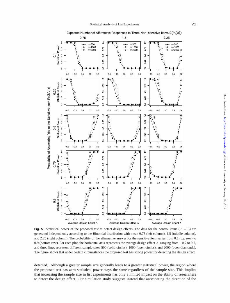
Statistical Analysis of List Experiments 71
Fig. 5 Statistical power of the proposed test to detect design effects. The data for the control items (J = 3) aregenerated independently according to the Binomial distribution with mean 0.75 (left column), 1.5 (middle column),and 2.25 (right column). The probability of the affirmative answer for the sensitive item varies from 0.1 (top row) to0.9 (bottom row). For each plot, the horizontal axis represents the average design effectΔ, ranging from−0.2 to 0.2,and three lines represent different sample sizes 500 (solid circles), 1000 (open circles), and 2000 (open diamonds).The figure shows that under certain circumstances the proposed test has strong power for detecting the design effect.
detected). Although a greater sample size generally leads to a greater statistical power, the region wherethe proposed test has zero statistical power stays the same regardless of the sample size. This impliesthat increasing the sample size in list experiments has only a limited impact on the ability of researchersto detect the design effect. Our simulation study suggests instead that anticipating the direction of the
at Princeton University on January 18, 2012
http://pan.oxfordjournals.org/D
ownloaded from

72 GraemeBlair and Kosuke Imai
designeffect and choosing appropriate control items are essential for efficiently detecting this type of listexperiment failure.
4 Concluding Remarks and Suggestions for Applied Researchers
Eliciting truthful answers to sensitive questions is one of the most important challenges for survey re-searchers. List experiments have recently emerged as an alternative to the randomized response techniquethat has been the most commonly used methodology for addressing this problem (seeWarner 1965;Gingerich 2010). The advantages of the list experiment over the randomized response method are inits simplicity, both for respondents and for the researcher. Most respondents find it easy to understandwhy list experiments provide them with some degree of privacy protection, while many find it difficultto see why randomization can protect privacy. In addition, unlike list experiments, which only involveseparate questions for different respondents, the randomized response method often requires survey re-spondents to conduct randomization without the supervision of enumerators, which can lead to logisticalchallenges and the difficulty of verifying accurate implementation. The simplicity of implementation ofthe list experiment comes with unique challenges: researchers must design list experiments such that theassumptions of no design effect and no liars are credible, and the statistical analysis of list experimentsrequire the modeling of both sensitive and control items.
Despite their growing popularity among applied researchers and their unique methodological chal-lenges, statistical analysis of list experiments has remained rudimentary. The set of new tools we developin this paper should help empirical researchers get the most out of list experiments. Here, we offer generalguidelines that can help applied researchers navigate the statistical analysis of list experiments:
• Estimate the proportion of each respondent “type” under the standard assumptions of list experi-ments as in the example in Table6. If there is a negative value, conduct the proposed statistical testfor detecting design effects (see Section3.1).
• Conduct multivariate regression analysis. We recommend the ML estimator for statistical efficiency,but linear and NLS provide slightly more robust alternatives at the cost of losing efficiency (seeSection2).
• Investigate the robustness of any conclusions to the potential existence of ceiling and/or floor effects.Start first by estimating the population proportion of liars using the intercept-only model and if thisproportion is large run a multivariate regression model that incorporates ceiling and/or floor effects(see Section3.2).
Finally, although this paper has focused upon the statistical analysis of list experiments, we emphasizethat the success of list experiments hinges upon their design. Only when careful design is combinedwith efficient statistical analysis can we effectively exploit the power of list experiments to elicit truthfulanswers from survey respondents. Thus, we conclude this paper by highlighting the following importantissues to which applied researchers should pay attention when designing list experiments (see alsoGlynn2010).
• To recoup the loss of information due to indirect questioning, use blocking or matched-pair designsbefore randomization. (Imai, King, and Stuart 2008).
• To avoid ceiling and floor effects, choose control items such that few respondents in the controlgroup would answer affirmatively or negatively to all control items. For example, researchers maychoose control items whose responses are negatively correlated with each other (Glynn 2010).
• To avoid design effects, choose control items whose evaluation is not affected by the inclusion ofsensitive items. For example, researchers should select control items that are unambiguous and forwhich respondents have strong opinions.
• Researchers should conduct a pilot study to assess the possibility of departures from the keyassumptions. The results of pilot studies can also be used to construct a design that maximizesthe power of the proposed statistical test for detecting design effects (see Sections3.1and3.5).
at Princeton University on January 18, 2012
http://pan.oxfordjournals.org/D
ownloaded from

StatisticalAnalysis of List Experiments 73
• To explore social desirability bias, it is useful to include direct questioning of the sensitive items.Such direct questioning can be administered to both treatment and control groups, but after indirectquestioning is done, through list experiments (see Section2.2).
• Asking control items directly can be useful for improving statistical efficiency, but researchersshould be aware of the possibility of introducing additional design effects. Presenting all con-trol items together first before asking each one separately may mitigate such design effects (seeSection2.4).
Mathematical Appendix
A.1 The Details of the ML Estimator of Section2.4
In this appendix, we derive the likelihood function based on the Poisson–Binomial distribution as dis-cussed in Section2.4. We also develop an EM algorithm to obtain the ML estimates of model parameters.For the sake of notational simplicity, we useZi,J+1 = Z∗
i,J+1. Formally, the distribution ofYi for respon-dent i in the treatment group is given by the Poisson–Binomial distribution with the following densityfunction:
Pr(Yi = y|Ti = 1, {π j (Xi , θ j )}J+1j =1)=
∑
z∈Z y
J+1∏
j =1
π j (Xi , θ j )Zi j (1 − π j (Xi , θ j ))
1−Zi j (A1)
for y = 0,1, . . . , J + 1, whereZ y ≡ {z = (Zi 1, . . . , Zi,J+1): Zi j ∈ {0,1}, andZi 1 + ∙ ∙ ∙ + Zi,J+1 = y}.Following Chen, Dempster, and Liu(1994), this density function can be written more compactly as
Pr(Yi = y|Ti = 1, {π j (Xi , θ j )}J+1j =1)= R(y, S; {π j (Xi , θ j )}
J+1j =1)
∏
j ∈S
(1 − π j (Xi , θ j )) (A2)
for y = 0,1, . . . , J + 1, where S = {1, . . . , J + 1} and R(k,C; {π j (Xi , θ j )}J+1j =1) ≡
∑B⊂C,|B|=k
(∏j ∈B
π j (Xi ,θ j )1−π j (Xi ,θ j )
)for any nonempty setC ⊂ S and 1 6 k 6 |C| with
R(0,C; {π j (Xi , θ j )}J+1j =1) = 1 and R(k,C; {π j (Xi , θ j )}
J+1j =1) = 0 for any k > |C|. Note thatR(k,C;
{π j (Xi , θ j )}J+1j =1) completelycharacterizes the distribution up to a normalizing constant. To evaluate this
function, we use a fast algorithm developed byChen, Dempster, and Liu(1994).Now, we can write the likelihood function under this modified design as follows:
L(θ | Y, T, X, {Z j }Jj =1) =
N∏
i =1
R(Yi , S; {π j (Xi , θ j )}
J+1j =1)
∏
j ∈S
(1 − π j (Xi , θ j ))
Ti
×
J∏
j =1
π j (Xi , θ j )Zi j (1 − π j (Xi , θ j ))
1−Zi j
1−Ti
.
(A3)
Due to the complex functional form of the Poisson–Binomial density function, the direct maximizationof this likelihood function is challenging. Thus, as before, we derive the EM algorithm for this setup byconsidering the answers for control items as missing data for the respondents in the treatment group.
In this case, the complete-data likelihood function is given by
Lcom(θ | T, X, {Z j }J+1j =1)
=N∏
i =1
πJ+1(Xi ; θ j )
Ti Zi,J+1(1 − πJ+1(Xi ; θ j ))Ti (1−Zi,J+1)
J∏
j =1
π j (Xi ; θ j )Zi j (1 − π j (Xi ; θ j ))
1−Zi j
.
(A4)
at Princeton University on January 18, 2012
http://pan.oxfordjournals.org/D
ownloaded from

74 GraemeBlair and Kosuke Imai
For each respondenti in the treatment group, the E-step of the EM algorithm requires the conditionalexpectation of missing dataZi j for j = 1, . . . , J + 1 given the observed data, that is,(Xi ,Yi ), and thecurrent parameter values{π j (Xi , θ j )}
J+1j =1. Chen,Dempster, and Liu(1994) derives the exact expression
for this conditional expectation as follows:
E(Zi j | Yi , Ti = 1, {π j ′(Xi , θ j ′)}J+1j ′=1})=
π j (Xi , θ j )R(Yi − 1,S\ { j }; {π j ′(Xi , θ j ′)}J+1j ′=1)
(1 − π j (Xi , θ j ))R(Yi , S; {π j ′(Xi , θ j ′)}J+1j ′=1)
, (A5)
for each j = 1, . . . , J + 1. We can calculate this quantity by again applying the efficient numericalalgorithm ofChen, Dempster, and Liu(1994). Finally, the M-step of the EM algorithm is simple andconsists of maximizing the weighted log-likelihood function for each regression modelπ j (x, θ j ), wherej = 1, . . . , J + 1.
A.2 TheDetails of the Hypothesis Test of Section3.1
We first derive the covariance matrix ofπ , which is denoted byΣ . Suppose that we use simple sam-ple analogue estimators,πy1 = 1
N0
∑Ni =1(1 − Ti )1{Yi 6 y} − 1
N1
∑Ni =1 Ti 1{Yi 6 y} and πy0 =
1N1
∑Ni =1 Ti 1{Yi 6 y} − 1
N0
∑Ni =1(1 − Ti )1{Yi 6 y − 1} for eachy. Now, for anyy 6 y′, we have
Cov(1{Yi 6 y}, 1{Yi 6 y′})= E[1{Yi 6 y}1{Yi 6 y′}] − E[1{Yi 6 y}]E[1{Yi 6 y′}] (A6)
= Pr(Yi 6 y){1 − Pr(Yi 6 y′)}. (A7)
Therefore,for any y 6 y′, the required covariance terms are given by
Cov(πy1, πy′1)=1∑
t=0
Pr(Yi 6 y | Ti = t){1 − Pr(Yi 6 y′ | Ti = t)}
Nt, (A8)
Cov(πy0, πy′0)=1∑
t=0
Pr(Yi 6 y − 1 + t | Ti = t){1 − Pr(Yi 6 y′ − 1 + t | Ti = t)}
Nt. (A9)
Eachof these covariance terms can be consistently estimated by their sample analogues.Given this expression, thep value is given by
pt =J∑
k=0
w(J, J − k, Σt )Pr(Vk > λt ), (A10)
whereVk is the chi-square random variable withk degrees of freedom, andw(J, J − k, Σt ) is the weightwhose expression is given inKudo (1963) andShapiro(1985) whenJ 6 4, a condition met by most listexperiments. WhenJ > 5, we employ a Monte Carlo approximation leveraging the fact thatw(J, J −k, Σt ) equalsthe probability ofπt having exactly J − k positive elements, whereπt is the solution toequation (20) andπt is distributed multivariate normal with mean zero and the covariance matrixΣ . Notethat if all the estimated proportions are nonnegative, that is,πyt > 0, thenλt = 0 and hencept = 1 fort = 0,1.
A.3 Derivation of the Sharp Bounds in the Presence of Ceiling and Floor Effects
First,note thatπJ1 satisfiesthe following constraints:
Pr(Yi = J + 1|Ti = 1)= (1 − q)πJ1, (A11)
Pr(Yi = J|Ti = 1)= πJ−1,1 + πJ0 + qπJ1, (A12)
Pr(Yi = J|Ti = 0)= πJ1 + πJ0. (A13)
at Princeton University on January 18, 2012
http://pan.oxfordjournals.org/D
ownloaded from

StatisticalAnalysis of List Experiments 75
Equations(A11) and (A13) imply that the lower and upper bounds onπJ1 equalto Pr(Yi = J +1|Ti = 1)and Pr(Yi = J|Ti = 0), respectively. Next, we investigate whether or not the information fromequation (A12) can improve these bounds. SinceπJ−1,1 is identified even in the presence of the ceil-ing and floor effects, we can rewrite equation (A12) as:
Pr(Yi 6 J|Ti = 1)− Pr(Yi 6 J − 1|Ti = 0)= πJ0 + qπJ1. (A14)
Now, equation (A13) is a linear combination of equations (A11) and (A14), and thus it follows thatequation (A12) does not improve the above bounds.
Similarly,π01 satisfiesthe following constraints:
Pr(Yi = 1|Ti = 1)= (1 − q)π01 + π10, (A15)
Pr(Yi = 0|Ti = 1)= π00 + qπ01, (A16)
Pr(Yi = 0|Ti = 0)= π00 + π01. (A17)
Even in the presence of the ceiling and floor effects, we can identifyπ10 andrewrite equation (A15) as
Pr(Yi = 0|Ti = 0)− Pr(Yi = 0|Ti = 1)= (1 − q)π01, (A18)
which implies that the lower bound ofπ01 is equal to Pr(Yi = 0|Ti = 0) − Pr(Yi = 0|Ti = 1).Equation(A17) implies that the upper bound is equal to Pr(Yi = 0|Ti = 0), and since equation (A16) isredundant given equations (A17) and (A18), it follows that these bounds cannot be further improved.
Together, these bounds imply the following sharp bounds on the population proportion of the respon-dents whose truthful answer is affirmative for the sensitive item
J∑
y=0
{Pr(Yi 6 y|Ti = 0)− Pr(Yi 6 y|Ti = 1)} 6 Pr(Z∗i,J+1 = 1),
6 Pr(Yi = 0|Ti = 0)+J−1∑
y=1
{Pr(Yi 6 y|Ti = 0)− Pr(Yi 6 y|Ti = 1)} + Pr(Yi = J|Ti = 0).
(A19)
Since the lower bound corresponds to the true population proportion for the sensitive item underAssumptions1 and2, the result confirms the intuition that the existence of ceiling and floor effects leadsto underestimation.
References
Andrews, D. W. K., and G. Soares 2010. Inference for parameters defined by moment inequalities using generalized moment selec-tion. Econometrica78:119–57.
Berinsky, A. J. 2004.Silent voices: Public opinion and political participation in America. Princeton, NJ: Princeton University Press.Biemer, P., and G. Brown. 2005. Model-based estimation of drug use prevalence using item count data.Journal of Official Statistics
21:287–308.Blair, G., and K. Imai. 2011a.list: Statistical Methods for the Item Count Technique and List Experiment. Comprehensive R Archive
Network (CRAN).http://CRAN.R-project.org/package=list.———. 2011b.Replication data for: Statistical analysis of list experiments. hdl:1902.1/17040. The Dataverse Network.Bullock, W., K. Imai, and J. N. Shapiro. 2011. Statistical analysis of endorsement experiments: Measuring support for militant
groups in Pakistan.Political Analysis19:363–84.Burden, B. C. 2000. Voter turnout and the national election studies.Political Analysis8:389–98.Chaudhuri, A., and T. C. Christofides. 2007. Item count technique in estimating the proportion of people with a sensitive feature.
Journal of Statistical Planning and Inference137:589–93.Chen, X., A. P. Dempster, and J. S. Liu. 1994. Weighted finite population sampling to maximize entropy.Biometrika81:457–69.Corstange, D. 2009. Sensitive questions, truthful answers? Modeling the list experiment with LISTIT.Political Analysis17(1):
45–63.Coutts, E., and B. Jann. 2011. Sensitive questions in online surveys: Experimental results for the randomized response technique
(RRT) and the unmatched count technique (UCT).Sociological Methods & Research40:169–93.
at Princeton University on January 18, 2012
http://pan.oxfordjournals.org/D
ownloaded from

76 GraemeBlair and Kosuke Imai
Dalton, D. R., J. C. Wimbush, and C. M. Daily. 1994. Using the unmatched count technique (UCT) to estimate base rates for sensitivebehavior.Personnel Psychology47:817–29.
Dempster, A. P., N. M. Laird, and D. B. Rubin. 1977. Maximum likelihood from incomplete data via the EM algorithm (withdiscussion).Journal of the Royal Statistical Society, Series B, Methodological39(1):1–38.
Droitcour, J., R. A. Caspar, M. L. Hubbard, T. L. Parsley, W. Visscher, and T. M. Ezzati. 1991. Measurement errors in surveys.In The Item Count Technique as a method of indirect questioning: A review of its development and a case study application, eds.P. P. Biemer, R. M. Groves, L. E. Lyberg, N. A. Mathiowetz, and S. Sudman, 185–210. New York: John Wiley & Sons.
Ehm, W. 1991. Binomial approximation to the Poisson binomial distribution.Statistics & Probability Letters11:7–16.Flavin, P., and M. Keane. 2009.How angry am I? Let me count the ways: Question format bias in list experiments. Technical Report,
Department of Political Science, University of Notre Dame.Gelman, A., A. Jakulin, M. G. Pittau, and Y. Su. 2008. A weakly informative default prior distribution for logistic and other regres-
sion models.Annals of Applied Statistics2:1360–83.Gilens, M., P. M. Sniderman, and J. H. Kuklinski. 1998. Affirmative action and the politics of realignment.British Journal of
Political Science28:159–83.Gingerich, D. W. 2010. Understanding off-the-books politics: Conducting inference on the determinants of sensitive behavior with
randomized response surveys.Political Analysis18:349–80.Glynn, A. N. 2010.What can we learn with statistical truth serum? Design and analysis of the list experiment. Technical Report,
Department of Government, Harvard University.Gonzalez-Ocantos, E., C. Kiewet de Jonge, C. Melendez, J. Osorio, and D. W. Nickerson. 2010.Vote buying and social desirability
bias: Experimental evidence from Nicaragua. Technical Report, Department of Political Science, University of Notre Dame.Holbrook, A. L., and J. A. Krosnick. 2010. Social desirability bias in voter turnout reports: Tests using the item count technique.
Public Opinion Quarterly74(1):37–67.Holland, P. W. 1986. Statistics and causal inference (with discussion).Journal of the American Statistical Association81:
945–60.Holland, B. S., and M. D. Copenhaver. 1987. An improved sequentially rejective Bonferroni test procedure.Biometrics43:
417–23.Imai, K. 2011. Multivariate regression analysis for the item count technique.Journal of the American Statistical Association
106:407–16.Imai, K., G. King, and E. A. Stuart. 2008. Misunderstandings between experimentalists and observationalists about causal inference.
Journal of the Royal Statistical Society, Series A (Statistics in Society)171:481–502.Janus, A. L. 2010. The influence of social desirability pressures on expressed immigration attitudes.Social Science Quarterly
91:928–46.Kane, J. G., S. C. Craig, and K. D. Wald. 2004. Religion and presidential politics in Florida: A list experiment.Social Science
Quarterly85:281–93.Kudo, A. 1963. A multivariate analogue of the one-sided test.Biometrika50:403–18.Kuklinski, J. H., M. D. Cobb, and M. Gilens. 1997a. Racial attitudes and the “New South.”Journal of Politics59:323–49.Kuklinski, J. H., P. M. Sniderman, K. Knight, T. Piazza, P. E. Tetlock, G. R. Lawrence, and B. Mellers. 1997b. Racial prejudice and
attitudes toward affirmative action.American Journal of Political Science41:402–19.LaBrie, J. W., and M. Earleywine. 2000. Sexual risk behaviors and alcohol: Higher base rates revealed using the unmatched-count
technique.Journal of Sex Research37:321–26.Manski, C. F. 2007.Identification for Prediction and Decision. Cambridge, MA: Harvard University Press.Miller, J. D. 1984. A new survey technique for studying deviant behavior. PhD diss, The George Washington University.Newey, W. K., and D. McFadden. 1994. Large sample estimation and hypothesis testing. InHandbook of Econometrics, ed.
R. F. Engle and D. L. McFadden, volume IV, 2111–245. Amsterdam, The Netherlands: North Holland.Perlman, M. D. 1969. One-sided testing problems in multivariate analysis.The Annals of Mathematical Statistics40:549–67.Presser, S., and L. Stinson. 1998. Data collection mode and social desirability bias in self-reported religious attendance.American
Sociological Review63:137–45.Raghavarao, D., and W. T. Federer. 1979. Block total response as an alternative to the randomized response method in surveys.
Journal of the Royal Statistical Society, Series B, Methodological41(1):40–5.Rayburn, N. R., M. Earleywine, and G. C. Davison. 2003. An investigation of base rates of anti-gay hate crimes using the unmatched-
count technique.Journal of Aggression, Maltreatment & Trauma6:137–52.Redlawsk, D. P., C. J. Tolbert, and W. Franko. 2010. Voters, emotions, and race in 2008: Obama as the first black president.Political
Research Quarterly63:875–89.Shapiro, A. 1985. Asymptotic distribution of test statistics in the analysis of moment structures under inequality constraints.
Biometrika72:133–44.Sniderman, P. M., and E. G. Carmines. 1997.Reaching Beyond Race. Cambridge, MA: Harvard University Press.Sniderman, P. M., P. E. Tetlock, and T. Piazza. 1992.Codebook for the 1991 National Race and Politics Survey. Survey Research
Center, Berkeley, California.http://sda.berkeley.edu/D3/Natlrace/Doc/nrac.htm.Streb, M. J., B. Burrell, B. Frederick, and M. A. Genovese. 2008. Social desirability effects and support for a female american
president.Public Opinion Quarterly72(1):76–89.Tourangeau, R., and T. Yan. 2007. Sensitive questions in surveys.Psychological Bulletin133:859–83.Tsuchiya, T. 2005. Domain estimators for the item count technique.Survey Methodology31(1):41–51.Tsuchiya, T., Y. Hirai, and S. Ono. 2007. A study of the properties of the item count technique.Public Opinon Quarterly71:
253–72.
at Princeton University on January 18, 2012
http://pan.oxfordjournals.org/D
ownloaded from

StatisticalAnalysis of List Experiments 77
Warner, S. L. 1965. Randomized response: A survey technique for eliminating evasive answer bias.Journal of the American Statis-tical Association60(309):63–9.
Wimbush, J. C., and D. R. Dalton. 1997. Base rate for employee theft: Convergence of multiple methods.Journal of AppliedPsychology82:756–63.
Wolak, F. A. 1991. The local nature of hypothesis tests involving inequality constraints in nonlinear models.Econometrica59:981–95.
Zaller, J. 2002. The statistical power of election studies to detect media exposure effects in political campaigns.Election Studies21:297–329.
at Princeton University on January 18, 2012
http://pan.oxfordjournals.org/D
ownloaded from