Statistical Analysis of Investment Costs for Power ...pure.iiasa.ac.at/4487/1/WP-95-109.pdf ·...

Working Paper Statistical Analysis of Investment

Costs for Power Generation Technologies

Manfred Strubegger and Irina Reitgruber

WP-95-109 November 1995

ASA International Institute for Applied Systems Analysis A-2361 Laxenburg Austria

.L 1. m...m Telephone: +43 2236 807 Fax: +43 2236 71313 E-Mail: [email protected]

Statistical Analysis of Investment Costs for Power Generation

Technologies

Manfred Strubegger and lrina Reitgruber

WP-95-109 November 1995

Working Papers are interim reports on work of the International Institute for Applied Systems Analysis and have received only limited review. Views or opinions expressed herein do not necessarily represent those of the Institute, its National Member Organizations, or other organizations supporting the work.

UllASA International Institute for Applied Systems Analysis A-2361 Laxenburg Austria

.L A. Dl... Telephone: +43 2236 807 Fax: +43 2236 71313 E-Mail: info~iiasa.ac.at

Strubegger and Reitgruber Statistical Analysis

Statistical Analysis of Investme~it Costs for Power Generation Technologies

Manfred Strubegger and lrina Reitgruber*)

1. Introduction

Differences i n the base assumptions and input data, more often than not, are the fundamental reason explaining the different results o f energy models. This paper analyzes variations i n investment cost data for electricity generation plants as found in different data sources ([I] t o [7]).

The analysis was carried out for the fol lowing ten types o f power generating technologies:

- coal power plants,

- coal gasification combined cycle plants,

- gas turbines,

- gas combined cycle plants,

- nuclear power plants,

- biomass and wood power plants,

- solar thermal power plants,

- photovoltaic power plants,

- wind power plants, and

- geothermal power plants

First we present a straight forward statistical analysis o f the collected investment cost data by applyig the method o f least sqares o n each type o f powerplant individually. Then these samples are further subdivided in to data groups for industrialized and developing countries. For the industrialized countries it was possible t o further disaggregate the data in to data sets w i th estimates for existing and future technologies.

*) TEMAPLAN, Vienna, Austria

Strubegger and Reitgruber Stat ist ical Analysis

In a second step the resulting cost ranges are used as input t o an energy model t o show the variat ion in the results of t ha t specific model, when the investment costs are varied w i th in t he suggested ranges f r o m the f i rst step.

Tools used T h e data and results shown i n this analysis are main ly based on t w o instruments:

- the C 0 2 mit igat ion technology data base ( C 0 2 D B [8]): Developed t o collect data fo r technologies relevant f o r mi t iga t ing C 0 2 emissions, C 0 2 can be used more generally t o collect and analyze data f o r a wide range o f energy technologies. Currently the data base contains some 1700 technologies, ranging f r o m resource extract ion technologies t o end use devices w i t h their economic, technical and ecological data. T h e C 0 2 D B served as data base fo r the investment costs of electricity generation technologies investigated i n th is analysis.

- the Model f o r Energy Supply Systems and their General Environmental Impact (MESSAGE [9]): A n opt imizat ion model fo r comparing various technologies w i t h respect t o their fitness i n the complete energy chain, tak ing i n to account their economic, technical and ecological parameters. MESSAGE was used t o analyze the efFect o f difFerent investment cost estimates o n the power generation systems. As an exemplary model, the global energy model used fo r the jo in t I lASA and W E C study [ lo] , consisting o f 11 interlinked wor ld regions w i t h a t i m e horizon o f up t o 2100 was used i n th is analysis.

3. Collected Data

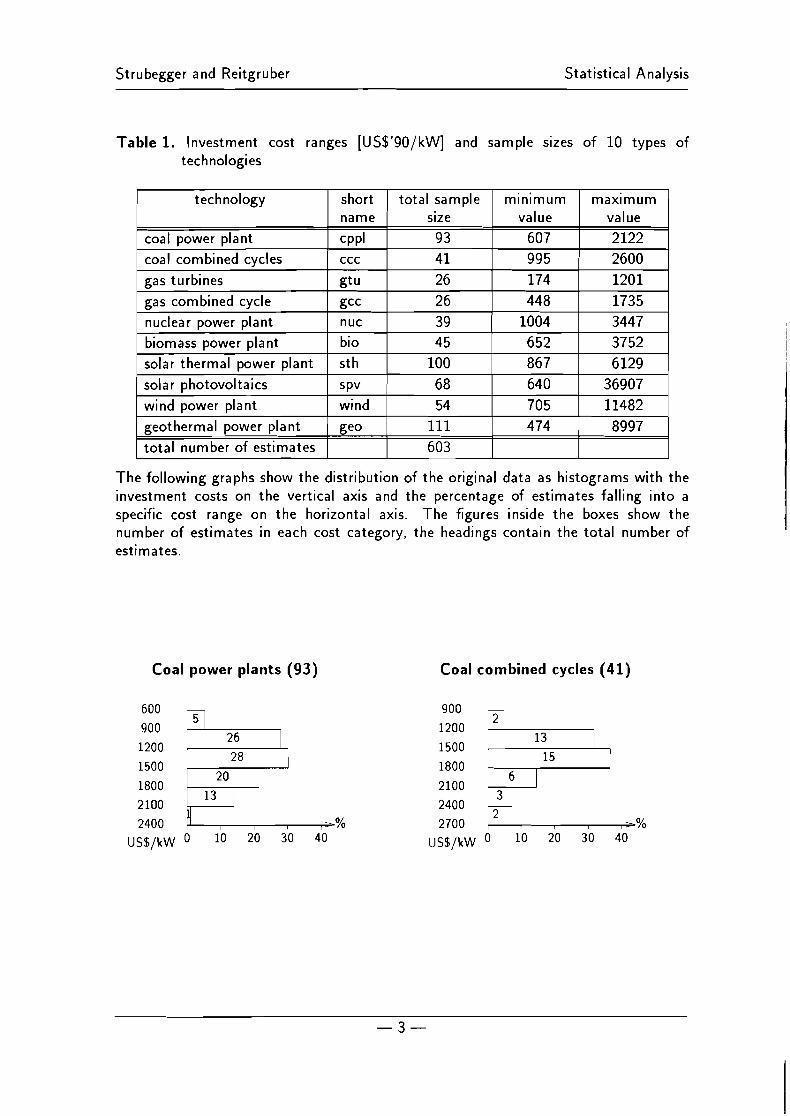
T h e data o f the C 0 2 D B stem f r o m various sources. T o minimize stat ist ical errors the data origin was traced and data derived f r o m the same original source were taken i n to account only once. Table 1 shows the sample size as well as the m in imum and max imum values o f t he specific investment costs fo r each o f t he technologies analyzed.


Table 1. Investment cost ranges [US$'90/kW] and sample sizes o f 10 types o f technologies

The following graphs show the distribution o f the original data as histograms with the investment costs on the vertical axis and the percentage of estimates falling into a specific cost range on the horizontal axis. The figures inside the boxes show the number o f estimates in each cost category, the headings contain the total number o f estimates.

Coal power plants (93) Coal combined cycles (41)


Gas turbines (26)

Gas combined cycles (26) 50 m

Nuclear power plants (39) Biomass power plants (45)

Solar thermal (100)


Wind power plants (54)

Al l cost distributions show a more or less pronounced ta i l towards the higher cost ranges. These tails, which cannot be explained by the analysis, seem t o reflect three facts:

Photovoltaics (68)

- matur i ty o f the technology,

700

1100 600 1500 2000 1900 3400 2300 4800 2700 6200 3100 7600 3500 9000 3900 10400 4300 11800 4700 13200 5100 14600 5500 16000 5900 17400 6300

- scalability, and

2 5 12

7

-

i i - 1 -

I I I I , =-%

- site dependence.

18800 USS/~W 0 10 20 30 40 50 20200

21600 Geothermal power plants (111)

23000

24400 0

25800 900

27200 1800

28600 2700

30000 3600

3 1400 4500

32800 5400

34200 6300

35600 7200

37000 % 8100

USS/kW 9000 % US$/kW O lo 20 30

Figure 1. Dis t r i bu t i on o f or ig inal est imates t o cost categories

Technologies producing electricity f r o m renewables show the longest tails, as these systems are i n their early development stages and are very site dependent. For the t w o


technologies with the longest tails (photovoltaicsl and wind), scalability - they can be built from very small t o fairly large units - expands the cost range into the higher categories (very small units are more expensive per kW installed capacity). Additionally, different accounting schemes may contribute to the shape of the distribution: The sources do not always state explicitly, if the given power is peak or average power, which of course results in drastically different cost estimates. The majority o f the estimates, however, refer t o peak capacity.

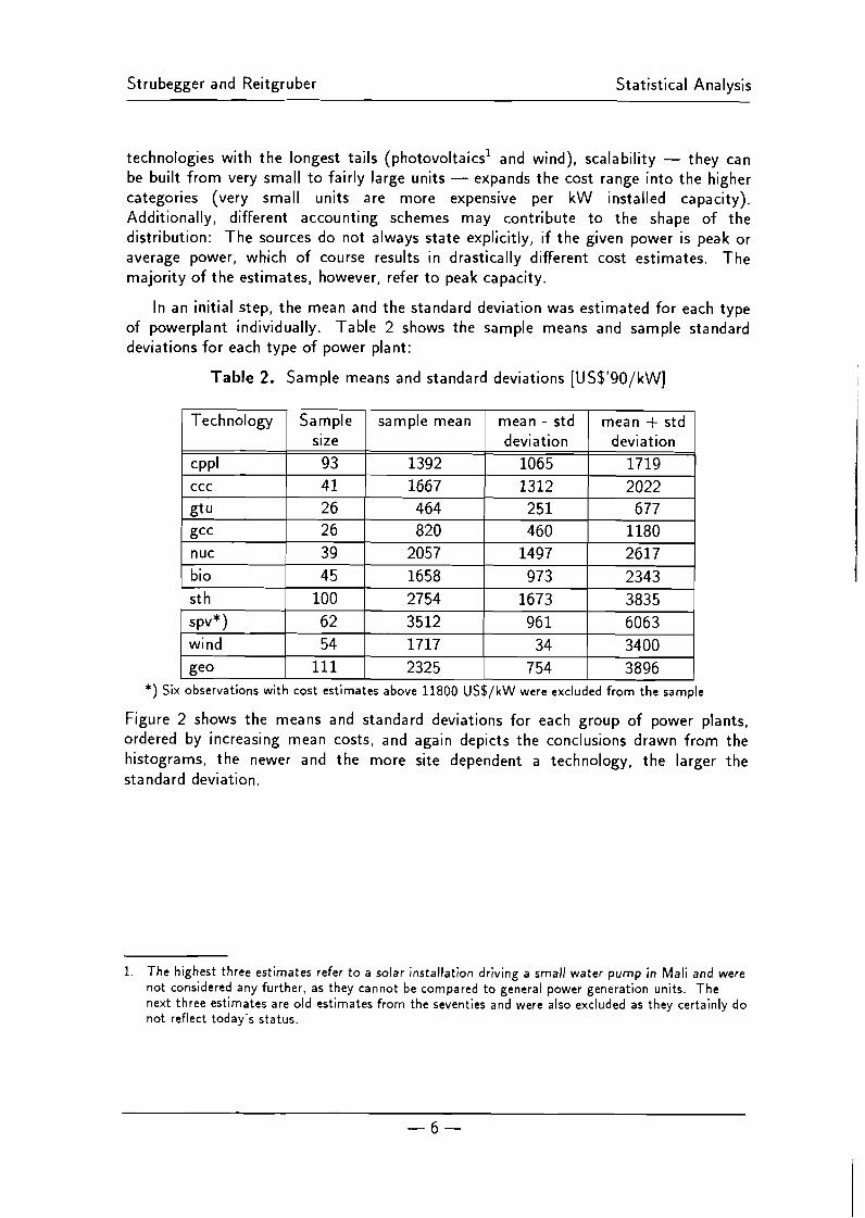
In an initial step, the mean and the standard deviation was estimated for each type of powerplant individually. Table 2 shows the sample means and sample standard deviations for each type of power plant:

Table 2. Sample means and standard deviations [US$'90/kW]

*) Six observat ions w i t h cos t est imates above 11800 U S S / k W were excluded f r o m t h e sample

Figure 2 shows the means and standard deviations for each group of power plants, ordered by increasing mean costs, and again depicts the conclusions drawn from the histograms, the newer and the more site dependent a technology, the larger the standard deviation.

1 . T h e highest th ree est imates refer to a solar instal lat ion dr iv ing a sma l l water p u m p i n M a l i and were n o t considered any fur ther , as t hey cannot be compared t o general power generat ion uni ts. T h e next th ree est imates are o l d est imates f r o m the seventies and were also excluded as they certainly d o n o t reflect today 's status.


Figure 2. Mean investment costs and standard deviations of original estimates

Figure 2 also shows, that a simple regression can not yield satisfactory results for giving realistic cost ranges for further model analysis. In many cases the compiled cost ranges show unrealistically low figures, reaching less than 50. US$/kW for wind power plants. In contrast, the lowest original estimate for wind power plants is 704 US$/kW. This is the result o f a method which assumes a normal distribution of the data. The data analyzed here do certainly not fulfill this criterion.

In order t o obtain more realistic results an econometric model based on the complete data set was built and estimated. This model and its results are described in the next sections.

4. An econometric model for the analysis of investment costs

T o utilize the information contained in C02DB, a two-step approach was taken t o derive plausible cost estimates with reasonable deviations from a mean value:

1. taking into consideration that the data chosen for this analysis stem from 18 data sources, it was statistically tested if a bias towards higher or lower estimates could be detected for individual data sources,

2. after correcting for potential biases, the analysis focused on trends related to the geographical location of the power plants, as well as to the t ime period for which the estimates were made.


4.1 Analysis of the data sources

Al l the data analyzed come f r o m 18 sources. Whi le many o f these sources provide investment cost estimates fo r only a few electricity generation technologies, some o f them give the estimates for almost all 10 technologies. T o est imate possible biases, the data sources giv ing estimates for a t least 6 different technologies were chosen (these are i tems [I ]- [7] i n the list o f references). Thus we divided the data in to 8 groups: while groups 1 t o 7 consist o f the data coming f r o m l i terature sources [I ]- [7] correspondingly, the last group contains the rest o f the data. The fol lowing econometric model was used for trend estimation:

Equation 1. Regression formula for data sources analysis

where:

I investment costs D i = l , . l O 0 - 1 variables for each o f the ten technologies

L i = l 7 0 - 1 variables for the seven complete data sources

L8 d u m m y variable for the remaining technologies

ti, li regression coefficients c error te rm

Almost all parameters associated w i th data sources [I] t o [7] turned ou t t o be statistically insignificant (all corresponding t-statistics were below 2). A n exception is the Report o f S tu t tgar t University [3] which provides cost estimates slightly below the average w i th a corresponding t - rat io on the border o f being significant (2.5). However, this can not seriously influence further statistical analysis o f the data, because only a small sample o f data comes f rom this source (one cost estimate for each technology). Therefore we can conclude tha t the main data sources, though providing a large variety o f diverging cost estimates, have no significant bias and can be used wi thout corrections fo r further statistical analysis o f the data.

4.2 Analysis of the investment data

T o provide a plausible est imate o f t he investment costs, statistical modeling can be used t o f ind factors influencing the costs in general (independent o f technology) and t o give quanti tat ive estimates o f this influence for each o f the technologies under consideration.


For this analysis the following two criteria were chosen:

- world region and

- time period for which an estimate was suggested.

T o ensure that enough data for statistical modeling remain in each group, we disaggregated in to two regional groups:

- industrialized and

- developing countries.

Concerning t ime periods the data were, for the same reason, also divided into two groups, where the group 'present' involves all the estimates made for years up t o 1995 and the group 'future' involves cost forecasts for all future years. Since the future cost estimates concern usually only developed countries, all data fall into three groups: present estimates for industrialized countries (ind), for developing countries (dev) and estimates for future costs in industrialized countries (fut). The size of these subsamples for each technology is shown in Table 3.

Table 3. Technology subgroups and their sample size

It seems economically plausible t o express the deviations in costs associated with developing countries or wi th future forecasts as percent differences t o the present cost estimates for the industrialized countries. Therefore all costs were transformed in to logarithms in order t o have an additive regression model. Moreover, transforming the data t o a logarithmic scale yields data sets conforming closer t o a normal distribution, which allows statistical analysis wi th general methods. Setting up the regression model for logarithmized costs includes the following three steps:

geothermal power plant

total number of estimates

- preliminary analysis o f the data distribution t o choose the model specification,

- estimation o f the model and

geo

- testing the residuals for independence (i.e. whether the model was correctly specified) and for normality (i.e. whether the assumption o f a logarithmic

111

597 55

360

28

135

28

102


distribution is valid).

4.3 Preliminary analysis of the logarithmized data

For the preliminary analysis of the logarithmized data, sample means and variances were computed for each data group and for each technology individually. -The corresponding diagrams are shown in Figure 3.

- ind fut dev ind fut dev ind fut dev ind fut dev ind fut dev

C P P ~ ccc gtu gCc nuc

ind fut dev ind fut dev ind fut dev ind fut dev ind fut dev bio sth S PV wind gee

Figure 3. Means and standard deviation in ln(US$'90/kW)

A brief view of the diagrams shows that the estimates for the developing countries exhibit somewhat lower means and higher variances than the ones for the industrialized countries. The three exceptions where the estimates for developing countries show somewhat higher values (coal combined cycles, gas combined cycles, and wind power plants), are, at least for a general conclusion, not plausible. While it may be possible that initial projects in developing countries may be more expensive due to the necessity t o buy technology and knowledge from industrialized countries, we see no reason why in the longer run the cost pattern should not follow that of the other technologies. A technology that calls for special attention are the geothermal power plants (the average for the developing countries su bsample is significantly lower than the one for the industrial group).

Concerning the projections, the diagrams show, that the means for future estimates are generally somewhat lower than the ones for present estimates with


possible exceptions o f nuclear and geothermal technologies (where they are somewhat higher) and photovoltaics (where they are essentially lower). These three groups also receive specific variables in the model.

Summarizing the discussions above, we suggest the following model for the investment cost analysis:

10

In(') = 1 aiDi + bDdev + cDfut + 1 di(DixDfut) + elo(DloxDdev)+'

i=1 i€5.8,10

Equation 2. Regression formula for data analysis

where

I ~nvestment costs D 1 , 1 0 0-1 variables for each o f the ten technologies

Ddev 0-1 variables indicating developing countries

D f ~ t 0-1 variables indicating estimates or future technologies

ai, b, c, di, ei regression coefficients e error term

The model reflects the fact that each investment cost estimate contains a component specific for the technology and a component specific for the data group (ind, dev or future). In addition, some technologies and data groups, for which the preliminary analysis showed that they do not follow the general trends, have a specific component (product o f the corresponding 0-1 variables). The regression coefficients o f these products indicate how much this particular group differs f rom the general trends.

4.4 Model estimation

The estimation o f the model consists o f two steps. First, it was estimated with the ordinary least square (OLS) method and the sample variances o f residuals for each subsample were computed. The estimated variances vary dramatically wi th the subsample: f rom 0.017 for nuclear power in industrialized countries t o 1.4 for wind power in developing countries. -The data obviously exhibit heteroscedastic behavior and the model was then reestimated wi th the generalized least square (GLS) method.

A t the second step (GLS) all the equations o f the model are weighted according t o the estimated standard deviations o f the residuals o f the corresponding subsamples. This leads t o the effect, that subsamples wi th higher standard deviations contribute less t o the parameters than subsamples wi th smaller standard deviations. The adjusted squared R statistics increase f rom 0.6 for the OLS step t o 0.925 for the GLS step. The following table gives the estimated values o f the parameters, their standard deviations and t-statistics.

Strubegger and Reitgruber Statistical Analysis - - - -

Table 4. Estimated model parameters (GLS)

The last column in table 4 shows the normalized values for the estimated parameters. The first ten values o f this column directly give the estimated costs for industrialized countries in US$'90/kW for all power plants included in this analysis. The following t w o values indicate the percentage cost differential for developing countries and future estimates, respectively. The last four values show the percentage cost differentials for the power plants treated specifically, and have t o be interpreted as percentage difference on top o f the difference shown for parameters b and c, respectively. Thus, e.g.:, future photovoltaics are some 45% (i.e.: (1-(1-.28)x(l-.23))x100.)* cheaper than present technology.

Para meter

a 1 cppl-ind

a 2 ccc-ind a 3 gtu-ind a4 gcc-ind a5 nuc-ind

a6 bio-ind

a 7 st h-ind as spv-ind a 9 wind-ind alo geo-ind

b d ev c f ~ t d5 nuc-fut d8 spv-fut dlo geo-fut

elo geo-dev

According t o the t-statistics all parameters are significant, so we proceed wi th the test.

4.5 Testing the residuals

Value Std. error t-statistics

7.28 0.027 271.587 7.41 0.035 212.264 6.19 0.078 79.750 6.72 0.081 83.017 7.61 0.029 261.432 7.37 0.061 120.678 7.92 0.040 195.809 8.32 0.128 64.934 7.27 0.062 118.090 7.73 0.070 110.701

-0.136 0.050 -2.728 -0.335 0.053 -6.339

pp

0.121 0.045 2.652 -0.255 0.093 -2.703

0.147 0.047 3.111 -0.427 0.126 -3.412

The GLS residuals were tested for independence and normality. W i t h testing for independence, we mean the test showing if for some o f the subsamples linear dependencies are left in the residuals ( that is certainly not a general test for independence). In other words we test the model (equation 2) against a model where each subsample has i ts own trend. W e build the following regression model for the

normalized

1451 1652 488 829

2018 1588 2752 4105 1437 2276 -13% -28%

+16% -35%

2 . see the last column of tab le 4


residuals: 10 10 10

2 = + I gi(DixDfut) + If i (DixDdev) + Y i=1 1=1 i=l

Equation 3. Regression model f o r residuals

T h e result o f this regression shows tha t none o f the est imated parameters s, g and f is significant (all t -stat ist ics are below 2.3.). Therefore the suggested model f r o m equation 2 is correct ly specified. T h e residuals were tested also f o r normal i ty w i t h t he Kolmogorov-Smirnov [9,10] test. T h e test results (see table 5) show, t h a t t he normal i ty hypothesis can be accepted.

Table 5. Results f r o m Kolmogorov-Smirnov test

sample slze: K S statistics: K S probabil ity: 0 .65

4.6 Conclusions to model estimation

T h e fac t t h a t t he suggested model proved t o be statistically reasonable ( the residuals can be considered independent and normally distributed) allows fo r the fo l lowing conclusions.

T h e model provides better qual i ty o f estimates f o r t h e suggested costs t han the results obtained by straight forward analysis o f the data. Tab le 6 gives a comparison of the standard deviation o f means fo r each group, computed f r o m the model and t h e corresponding subsamples. T h e estimates f o r industrialized countries have similar values, whereas fo r developing countries and f o r fu ture costs t he standard deviations resulting f r o m the model are essentially smaller. T h e model gives also a possibility of est imat ing the costs (and standard deviations) f o r groups were no data are available ( future biomass power plants and solar thermal and solar photovoltaic power plants i n developing countries). T h e values of t h e means computed f r o m the original estimates and f r o m the model are given i n table 7.


Table 6. Standard deviation o f mean: model estimates and sample values

Technology

C P P ~ CCC

gtu gee nuc bio sth

SPV wind geo

stdd(mean), dev

model I sample

2 2 *) calculated f r o m : ecppl+2xecpp,,xe,t*cf,,,,cPPI+e,Ut; w i t h e being the s tandard error ( table 4) and c t he corresponding coe f f~c ien t f r o m the correlat ion m a t r i x o f regression coefficients.

Table 7. Mean: model estimates and sample values

2. The analysis proved that the logarithms o f the investment costs are normally distributed (with means and variances different for each of the subgroups). This allows t o estimate not only means, but also confidence intervals for the means. These intervals give reasonable lower and upper bounds for the suggested cost estimates. T o compute these statistics for investment costs directly is difficult, because o f the complex distribution of the investment costs (they are exponents o f normally distributed random variables). Therefore we compute the statistics for logarithmized costs and then transform the intervals. Table 8 shows values for means and means +/$-$ standard deviation transformed into investment costs (in US$'gO/kW). The figures in table 8 compare t o the ones shown in table 2 for the initial analysis.

Technology

C P P ~

ccc

gtu gCC nuc bio sth

SPV wind

gee

mean, ind mean, dev

model

7.277 7.408 6.182 6.720 7.609 7.369 7.925 8.322 7.277 7.733

mean, future

model

7.141 7.272 6.046 6.584 7.473 7.233 7.789 8.186 7.141 7.170

sample

7.286 7.372 6.201 6.637 7.607 7.359 7.948 8.438 7.430 7.733

model

6.942 7.073 5.847 6.385 7.396 7.034 7.590 7.732 6.942 7.545

sample

6.983 7.322 6.068 6.692 7.524 7.277 -

-

7.659 7.023

sample

7.201 7.185 5.682 6.490 7.624 -

7.491 7.521 6.909 7.763


Table 8. lnvestment costs: mean and mean +/- standard deviation [US$'90/kW]

Table 9 shows the values calculated for a 95% confidence interval (from min t o max). These are finally the cost ranges suggested for use in mathematical energy models investigating the competitiveness of power plants in the global electricity market.

Table 9. lnvestment costs: 95% confidence intervals for means [US$'90/kW]

r

Technology

C P P ~ ccc

gtu gCC nuc bio

wind

1 gee

Technology

C P P ~

CCC

gt" gee nuc bio sth

SPV wind

g@='

ind future(ind)

ind

min

1145 1285

363 610

1577 1200 2134 2745 1086 1048

d ev

mean

1035 1180

346 593

1629 1135

3. There are general trends associated with the cost estimates for the future and for developing countries. Namely, in developing countries the costs are about 13% lower than in the industrialized countries. The only important exception are geothermal power plants, where this estimate is 43% lower. It only can be guessed, that this significantly lower estimate is based on different geological conditions in developing countries as compared t o industrialized countries.

mean+ stddev

1486 1708 523 899

2076 1686 2878 4675 1539 2448

mean

1263 1439 422 723

1760 1384

mean

1447 1649 484 829

2016 1586 2766 4113 1447 2282

future(ind)

The future costs in industrialized countries are approximately 28% lower than the present ones for most o f the technologies. For geothermal power plants the future drop in costs is expected t o be around 17% only (probably due t o the fact that these costs depend on the geographic location and natural conditions, and that the cheapest locations will no longer be available in the future). For nuclear power plants the relatively small decrease in future costs (19%) can be associated t o increasing safety requirements, which lead t o cost increases. Fast progress is expected for photovoltaics: about 45% decrease in costs, which can

mean- stddev

1408 1592 448 764

1959 1492 2657 3619 1360 2128

1978 2280 1035 1891

mean- stddev

978 1112 317 541

1541 1047

d ev

mean+ stddev

1094 1251

378 649

1723 1229

mean- stddev

1201 1358

391 663

1664 1287 2267 3131 1169 1164

1867 1947 990

1779

mean+ stddev

1327 1525 456 789

1861 1489

2 5 7 1 4117 1 1364 1451

2096 2414 2670 1 3 5 9 0 1081 2010

1263 1300


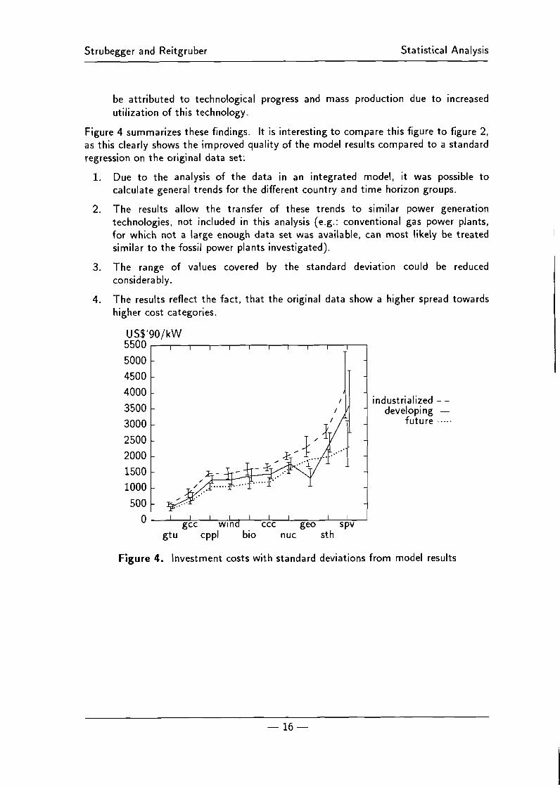
be at t r ibuted t o technological progress and mass production due t o increased ut i l izat ion o f th is technology.

Figure 4 summarizes these findings. I t is interesting t o compare th is figure t o figure 2, as this clearly shows t h e improved quality o f t he model results compared t o a standard regression o n t h e original data set:

1. Due t o the analysis o f t he data i n an integrated model, it was possible t o calculate general trends for t he different country and t i m e horizon groups.

2. T h e results al low the transfer o f these trends t o similar power generation technologies, not included in this analysis (e.g.: conventional gas power plants, f o r which no t a large enough data set was available, can most likely be treated similar t o the fossil power plants investigated).

3. T h e range o f values covered by the standard deviation could be reduced considerably.

4. T h e results reflect the fact, tha t the original data show a higher spread towards higher cost categories.

industrialized developing

future

0 1 I I I I I I I I I I gcc WI nd ccc geo spv

g t u cppl bio nuc st h

Figure 4. Investment costs w i th standard deviations f r o m model results


5. Applications of the estimated investment costs

The influence o f the estimated investment costs o f power generating technologies on the global electricity supply structure was studied by applying the estimated figures f rom this study t o the global version o f the MESSAGE energy supply model.

T o test the influence o f parameter changes, a standard version o f the model was taken, together wi th all i ts input data for other technologies, such as energy extraction plants and equipment, energy conversion, transport/distribution, and end-use technologies, remaining in place. Based on this setup t w o test change cases were produced:

1. a test w i th the initial overall estimates f rom table 2, and

2. a test w i th the disaggregated estimates f rom table 9.

For the second test, the estimated parameters were adapted t o reflect possible development paths: First, the investment costs for the 10 technologies were adopted t o the estimated mean values for industrialized and developing countries. For the dynamics o f the investment costs, it was assumed, that for industrialized countries the costs decrease exponentially up t o the year 2020, so that in 2020 they achieve the target resulting f rom the statistical model. For most technologies the reduction is 28%, for nuclear, geothermal and photovoltaics it reaches 19%, 17% and 45% respectively. After 2020 the decrease in costs for mature technologies (coal, gas, low cost nuclear) is supposed t o stop due t o absence o f further technological improvements in this field, whereas for new technologies (solar, geo, bio, wind, high cost nuclear) the costs will further experience a decline, though at a lower rate.

For the developing countries, the following cost dynamics was assumed: for mature technologies the costs approach those estimated for the year 2040 in the industrialized countries. Afterwards they follow the same path as the costs for industrialized countries now. This reflects the fact, that the lower estimates for developing countries are based on less costly technologies wi th lower environmental standards. Establishing better environmental standards increases the cost o f power generation equipment, which offsets cost decreases initially, only when current standards are met, the investment costs can pick up decreases due t o technological progress. For new technologies the cost dynamics in developing countries was assumed t o be the same as in industrialized countries, assuming, that technological progress is transferred t o the developing countries. However, as wi th mature technologies, the final price is the one for the future in industrialized countries, i.e.: the cost differential disappears.

The Reforming Countries are treated the same as industrialized countries.

The following figures show the results for electricity generation by technology for the t w o change cases. The graphic on the left hand always shows the development wi th constant investment costs, the one at the right hand side the development wi th decreasing investment costs.


GWyr OECD c o n s t 3000

2500

2000

1500

1000

500

0

GWyr OECD dyn gee -3-

wind .+. . . spv -D- sth x -

hydro A- nuc .x . . . bio -+ - gcc + -

~ P P I %- oil .x.. .

CCC a - cppl -m -

Figure 5. Electricity production in industrialized countries without (left) and with (right) changing investment costs [GWyr]

The comparison for the industrialized countries shows, that, starting around 2020, the cost changes favour the systems using renewable energy forms (curves towards the top o f the graph). This is, o f course, no big surprise, as these systems are at the beginning o f the i r life cycle and thus will profit f rom sharper cost decreases than todays mature technologies. By the end o f the t ime horizon, the electricity output o f these systems double compared t o the case with no price changes. When examining the fossil technologies (curves at the lower end o f the graph), one sees, that advanced coal systems (like combined cycles) can replace the conventional coal power plants by the middle o f next century. In both tests the bulk production comes from natural gas converted in gas corn bined cycles.

GWyr REF c o n s t 1400

GWyr REF dyn 1400 geo +

wind .+... 1200 SPV a-

sth *- 1000 hydro A-

nuc . X . . . bio + - gcc + -

~ P P I -E- oil .x.. .

CCC a - cppl *-

2000 2020 2040 2060 2080 2100 2000 2020 2040 2060 2080 2100

Figure 6. Electricity production in reforming countries without (left) and with (right) changing investment costs [GWyr]

The picture for the reforming countries reveals a similar structure as the one for the industrialized countries. The difference being, that the share o f natural gas in the supply menu is reduced in favour t o the higher production from environmentally more benign ways t o generate electricity.


GWyr DEV const GWyr DEV dyn gee ++

wind .+. . . spv G - sth s-

hydro a nuc .f.. . bio + - gcc +-

gppl + oil .x.. .

CCC a - cppl r-

Figure 7. Electricity production in developing countries without (left) and with (right) changing investment costs [GWyr]

In the developing countries, only production from coal is somewhat reduced due t o the shifts in production costs. The overall production structure hardly changes, as the developing countries have hardly any degrees o f freedom. Being mostly supply constrained and being faced with a rapidly increasing demand all energy carriers have t o be utilized close t o their potential. Moreover, the cost changes are smaller, than in the industrialized countries, as the cost decreases are partially offset by the need t o install cleaner power plants with higher costs than so far.

Summarizing, it can be said, that the price changes for electricity production equipment leads t o a more balanced production pattern in all three regions and increases the potential t o produce more electricity f rom sources with strongly reduced C 0 2 emissions.

Summarizing, these differences between the two test cases is shown in figure 8, where electricity production is aggregated into the primary energy categories fossil, nuclear and renewable. Here one can see clearly, that the share o f electricity generated from renewable sources nearly doubles, if the estimated investment cost figures are used rather than constant values over the complete t ime horizon.


Figure 8. Global electricity production without (left) and with (right) changing investment costs [shares]

100%

90%

80%

70%

60%

50%

40%

30%

20%

10%

0 %

2020 2050 2100

6. Final remarks

100%

90%

80%

70%

60%

50% Nuclear

40%

30%

20%

10%

0 %

2020 2050 2100

The method described in this paper allows t o generate cost ranges for ten types o f power plants based on a fairly large set o f 603 independent estimates. By this it was possible t o estimate costs for these power plants for different world regions and t ime periods. Model applications using theses data have shown, that the results improve, compared t o runs, were constant cost figures were used for all regions over the complete t ime horizon.

As this experiment proved t o produce valuable results, similar investigations should be performed for other variables, like efficiencies o f power plants and costs o f other technologies in the energy chain. The most l imi t ing factor is the availability o f a large enough data set t o allow a meaningful disaggregation o f the data t o more regions and t ime periods. As one can see f rom this study some 600 estimates were needed t o provide estimates for t w o regions and two t ime steps.


References

1. J.R. Ybema, P.A.Okken, T. Kram, P.Lako, C02 Abatement in the Netherlands,

Report, ECN, 1993.

2. M.A. Bernstein, Costs and Greenhouse Gas Emissions o f Energy Supply and Use, Report submitted t o the World Bank, Center for Energy and the Environment, University o f Pennsylvania, 1992.

3. U. Fahl, R. Kuehner, P. Liebscher, G. Schmid, A. Voss, Referenzszenario des Energiebedarfs und der Emissionen, Final report, IKE, University Stuttgart, 1990.

4. Technical Assessment Guide - Electricity Supply 1989., Report, Electric Power Research Institute, USA, 1989.

5. The IPCC Technology Characterization Inventory, Phase II Report, Volume I and Volume II ,IPCC, DOE o f USA, 1993.

6. Senior Expert Symposium on Electricity and the Environment, Comparative Assessment o f Electricity Generating Technologies (Key Issues Paper No. 2), Report, IAEA, 1991, Key Issues Papers for a Senior Expert Symposium held in Helsinki, Finland, 13-17 May 1991.

7. The Potential o f Renewable Energy, Report, Prepared for the Office o f Policy, Planning and Analysis, US DOE, Contract No. DE-AC02-83CH10093, 1991.

8. S. IVlessner, M . Strubegger, User's Guide t o C 0 2 D B : The IIASA CO, Technology Data Bank, Version 1.0, WP-91-31a, IIASA, Laxenburg, Austria, 1991.

9. S. Messner, M . Strubegger, User's Guide for MESSAGE 111, WP-95-69, IIASA, Laxenburg, Austria, 1995.

10. I IASA/WEC (World Energy Council), Global Energy Perspectives t o 2050 and Beyond , WEC, London, LlK, 1995.

11. Bronstein, Semendjajew, Taschenbuch der Mathematik, BSB B.G. Teubner Verlagsgesellschaft, Leipzig, 1983.

12. SYSTA T The System for Statistics, SYSTAT, inc., 1987.

Statistical Analysis of Investment Costs for Power ...pure.iiasa.ac.at/4487/1/WP-95-109.pdf ·...

Documents

Transcript of Statistical Analysis of Investment Costs for Power ...pure.iiasa.ac.at/4487/1/WP-95-109.pdf ·...