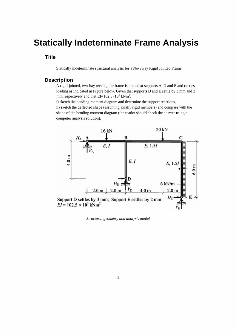
1

Statically Indeterminate Frame Analysis

Title

Statically indeterminate structural analysis for a No-Sway Rigid Jointed Frame

Description A rigid-jointed, two-bay rectangular frame is pinned at supports A, D and E and carries

loading as indicated in Figure below. Given that supports D and E settle by 3 mm and 2

mm respectively and that EI=102.5×103 kNm2;

i) sketch the bending moment diagram and determine the support reactions,

ii) sketch the deflected shape (assuming axially rigid members) and compare with the

shape of the bending moment diagram (the reader should check the answer using a

computer analysis solution).

Structural geometry and analysis model

2

Finite Element Modelling:

Analysis Type: 2-D static analysis (X-Z plane)

Step 1: Go to File>New Project and then go to File>Save to save the project with any name

Step 2: Go to Model>Structure Type to set the analysis mode to 2D (X-Z plane)

Unit System: kN,m

Step 3: Go to Tools>Unit System and change the units to kN and m.

3

Geometry generation:

Step 4: Go to Model>Structure Wizard>Beam and type 2.0,2.0,4.0,2.0 in the Distances

box. Press Apply. Switch to the Front view by clicking on as shown below. Switch on

node number from the option . Node number 1 will be point A.

Step 5: Go to Model>Elements>Extrude Elements. Select type as Node->Line. Use select

single button to highlight the node number 3 by clicking on it. Type in (0,0,-4) in the

Equal Distances dx,dy,dz box and enter number of times=1 and click Apply to generate the

column BD.

4

Step 6: Similar to Step 5, select this time node number 5 and enter dx,dy,dz as (0,0,-6) m,

number of times=1 and click Apply to generate the second column CE.

Material: EI= 102.5*103 kNm2. Let us consider Modulus of elasticity, E = 102.5 × 103

kN/m2. Then I will be 1.0 m4.

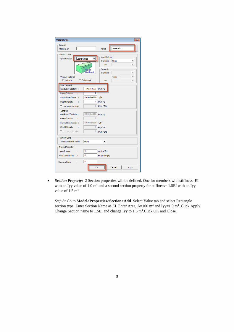
Step 7: Go to Model>Properties>Material>Add. Select User defined in the Type of Design

and Enter E=102.5 × 103 kN/m2. Enter a name for the material and click OK and Close.

5

Section Property: 2 Section properties will be defined. One for members with stiffness=EI

with an Iyy value of 1.0 m4 and a second section property for stiffness= 1.5EI with an Iyy

value of 1.5 m4

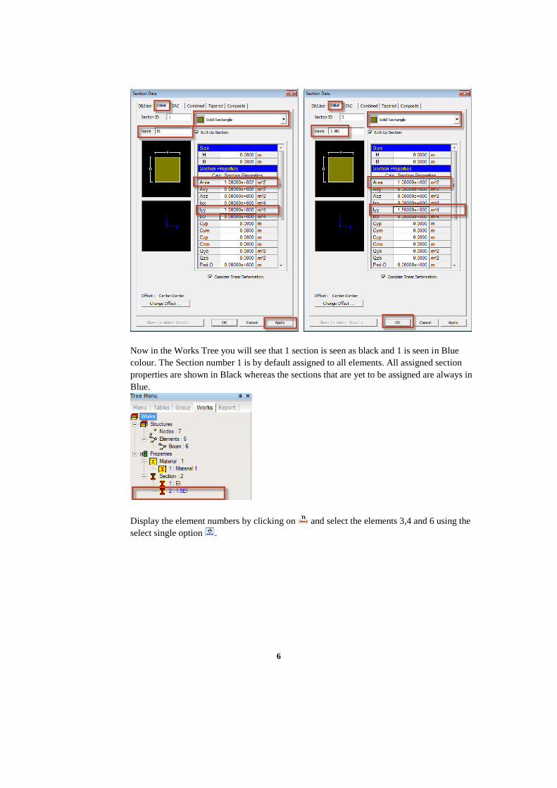
Step 8: Go to Model>Properties>Section>Add. Select Value tab and select Rectangle

section type. Enter Section Name as EI. Enter Area, A=100 m4 and Iyy=1.0 m4. Click Apply.

Change Section name to 1.5EI and change Iyy to 1.5 m4.Click OK and Close.

6

Now in the Works Tree you will see that 1 section is seen as black and 1 is seen in Blue

colour. The Section number 1 is by default assigned to all elements. All assigned section

properties are shown in Black whereas the sections that are yet to be assigned are always in

Blue.

Display the element numbers by clicking on and select the elements 3,4 and 6 using the

select single option .

7

Boundary Condition: Pinned Supports at A, D and E.

Step 9: Use select single to select or highlight nodes 1,6 and 7 as shown in figure below.

Go to Model>Boundaries>Supports and check on Dx and Dz and Apply.

8

These become the Pinned supports at A,D and E. DX and DZ provide horizontal and

vertical restraint simultaneously. No rotational restraint has been provided.

Load Case:

Concentrated Loads:

-Vertically downward loads of 16 kN and 20 kN on the members AB and BC respectively

applied in (-Z) direction.

-Horizontally applied uniformly distributed load (UDL) of 6kN/m applied on the member

CE in the (-X) direction.

-Settlements of 3mm and 2mm applied at the supports D and E respectively in the (-Z)

direction.

Step 10: Go to Load>Static Load Cases and define static load case ‘P’. Select Load type as

User defined for both of them. Click Close after adding the load case.

Step 11: Go to Load>Nodal Loads and select load case P. Select the node 2 using and

enter FZ=-16 kN and press Apply. Select Node 4 and enter FZ=-20 kN and Apply.

9

You can display the values from the Works Tree by Right clicking on Nodal Loads and click

Display.

Uniform Loads: A uniformly distributed load, UDL of 12 kN/m is applied vertically

downward on the member CD.

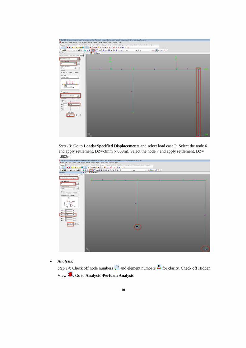
Step 12: Go to Loads>Element Beam Loads and select load case P. Select the element

number 6 and enter w=-6 kN/m in the Global X direction and press Apply and Close.

10

Step 13: Go to Loads>Specified Displacements and select load case P. Select the node 6

and apply settlement, DZ=-3mm (-.003m). Select the node 7 and apply settlement, DZ=

-.002m.

Analysis:

Step 14: Check off node numbers and element numbers for clarity. Check off Hidden

View . Go to Analysis>Perform Analysis

11

Results

Reaction Forces:

Step 15: Click on Results>Reactions>Reaction Forces/Moments and select the load case

P. Select FXYZ. Check on Values and click on the box next to Values to change number

of decimal points to 2 and click OK to see reactions graphically.

Deformations:

Step 16: Go to Results>Deformations>Deformed Shape. Select load case P. Select DXYZ.

Check on Values and Undeformed. Click on the box next to Deform and increase scale

factor to 3 and set to real deformation and click OK.

12

Beam forces/moment diagrams:

Step 17: Click on Results>Forces>Beam Diagrams and select the load Case P. Select My

and Click Apply to display the bending moment diagram in the members. Select Min/Max

to display the minimum and maximum bending moment values on the members.

13

Hand Calculations:

Moment Distribution Method will be used to calculate the bending moments.

Fixed-end Moments:

The final fixed-end moments are due to the combined effects of the applied member

loads and the settlement; consider the member loads,

Member AB:

Fixed end moments

M𝐴𝐵 = −𝑃𝐿

8= −

16×4

8= −8 kNm

MBA = +PL

8= +

16 × 4

8= +8 kNm

Since support A is pinned, the fixed-end moments are (MBA−0.5MAB) at B and zero at A.

(M𝐵𝐴 − M𝐴𝐵 2⁄ ) = [+8 + (0.5 × +8)] = +12 kNm

Member BC:

M𝐵𝐶 = −𝑃𝑎𝑏2

𝐿2= [− (

20.0 × 4.0 × 2.02

62)] = −8.9 𝑘𝑁𝑚

M𝐶𝐵 = +𝑃𝑎2𝑏

𝐿2= [+ (

20.0 × 4.02 × 2.0

62)] = −17.8 𝑘𝑁𝑚

14

Member CE:

M𝐶𝐸 = −𝑤𝐿2

12= −

6.0 × 62

12= −18.0 𝑘𝑁𝑚

M𝐸𝐶 = +𝑤𝐿2

12= +

6.0 × 62

12= +18.0 𝑘𝑁𝑚

Since support E is pinned, the fixed-end moments are (MCE−0.5MEC) at C and zero at E.

(M𝐶𝐸 − 0.5M𝐸𝐶) = −18.0 − (0.5 × +18.0) = −27.0 𝑘𝑁𝑚

Consider the settlement of supports D and E: δAB=3.0 mm and δBC=1.0 mm

𝑀𝐵𝐴 = −3(𝐸𝐼𝛿𝐴𝐵)

𝐿𝐴𝐵2 = −

3(102.5 × 103 × 0.003)

4.02= −57.6 𝑘𝑁𝑚

Note: the relative displacement between B and C i.e. δBC=(3.0–2.0)=1.0 mm

𝑀𝐵𝐶 = +6(𝐸1.5𝐼𝛿𝐵𝐶)

𝐿𝐵𝐶2 = +

6(1.5 × 102.5 × 103 × 0.001)

6.02= +25.6 𝑘𝑁𝑚

Final Fixed End Moments:

Member AB: 𝑀𝐴𝐵 = 0 𝑀𝐵𝐴 = +12.0 − 57.6 = −45.6 𝑘𝑁𝑚

Member BC: 𝑀𝐵𝐶 = −8.9 + 25.6 = +16.7 𝑘𝑁𝑚 𝑀𝐶𝐵 = +17.8 + 25.6 = +43.4 𝑘𝑁𝑚

Member CE: 𝑀𝐶𝐸 = −27.0 𝑘𝑁𝑚 𝑀𝐸𝐶 = 0

Distribution Factors: Joint B

𝑘𝐵𝐴 = (3

4×

𝐼

4.0) = 0.19𝐼

𝐷𝐹𝐵𝐴 =

𝑘𝐵𝐴

𝑘𝑡𝑜𝑡𝑎𝑙

=0.19

0.63= 0.3

𝑘𝐵𝐶 = (1.5𝐼

6.0) = 0.25𝐼

𝑘𝑡𝑜𝑡𝑎𝑙 = 0.63𝐼 𝐷𝐹𝐵𝐶 =

𝑘𝐵𝐶

𝑘𝑡𝑜𝑡𝑎𝑙

=0.25

0.63= 0.4

𝑘𝐵𝐷 = (3

4×

𝐼

4.0) = 0.19𝐼

𝐷𝐹𝐵𝐷 =

𝑘𝐵𝐷

𝑘𝑡𝑜𝑡𝑎𝑙

=0.19

0.63= 0.3

15

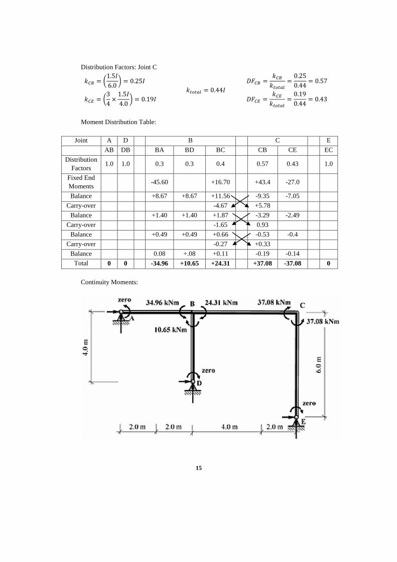
Distribution Factors: Joint C

𝑘𝐶𝐵 = (1.5𝐼

6.0) = 0.25𝐼

𝑘𝑡𝑜𝑡𝑎𝑙 = 0.44𝐼

𝐷𝐹𝐶𝐵 =𝑘𝐶𝐵

𝑘𝑡𝑜𝑡𝑎𝑙

=0.25

0.44= 0.57

𝑘𝐶𝐸 = (3

4×

1.5𝐼

4.0) = 0.19𝐼 𝐷𝐹𝐶𝐸 =

𝑘𝐶𝐸

𝑘𝑡𝑜𝑡𝑎𝑙

=0.19

0.44= 0.43

Moment Distribution Table:

Joint A D B C E

AB DB BA BD BC CB CE EC

Distribution

Factors 1.0 1.0 0.3 0.3 0.4 0.57 0.43

1.0

Fixed End

Moments -45.60 +16.70 +43.4 -27.0

Balance +8.67 +8.67 +11.56 -9.35 -7.05

Carry-over -4.67 +5.78

Balance +1.40 +1.40 +1.87 -3.29 -2.49

Carry-over -1.65 0.93

Balance +0.49 +0.49 +0.66 -0.53 -0.4

Carry-over -0.27 +0.33

Balance 0.08 +.08 +0.11 -0.19 -0.14

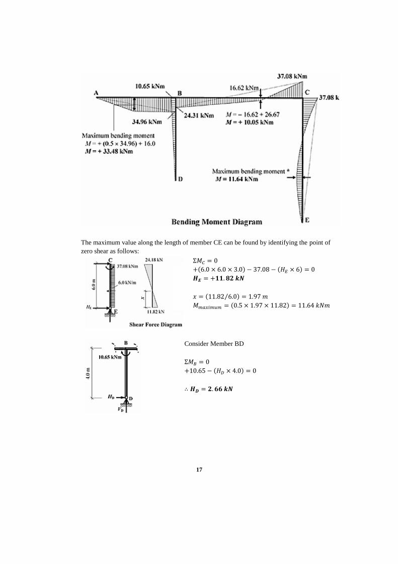
Total 0 0 -34.96 +10.65 +24.31 +37.08 -37.08 0

Continuity Moments:

16

Free Bending Moments:

Member AB: Member BC:

𝑀𝑓𝑟𝑒𝑒 =𝑃𝐿

4=

16 × 4

4= 16 𝑘𝑁𝑚 𝑀𝑓𝑟𝑒𝑒 =

𝑃𝑎𝑏

𝐿=

20 × 4 × 2

6= 26.67 𝑘𝑁𝑚

Member CE:

𝑀𝑓𝑟𝑒𝑒 =𝑤𝐿2

8=

6 × 6.02

8= 27 𝑘𝑁𝑚

17

The maximum value along the length of member CE can be found by identifying the point of

zero shear as follows:

Σ𝑀𝐶 = 0 +(6.0 × 6.0 × 3.0) − 37.08 − (𝐻𝐸 × 6) = 0

𝑯𝑬 = +𝟏𝟏. 𝟖𝟐 𝒌𝑵

𝑥 = (11.82 6.0⁄ ) = 1.97 𝑚

𝑀𝑚𝑎𝑥𝑖𝑚𝑢𝑚 = (0.5 × 1.97 × 11.82) = 11.64 𝑘𝑁𝑚

Consider Member BD

Σ𝑀𝐵 = 0

+10.65 − (𝐻𝐷 × 4.0) = 0

∴ 𝑯𝑫 = 𝟐. 𝟔𝟔 𝒌𝑵

18

Consider a section B:

Σ𝑀𝐵 = 0

+24.31 + (20.0 × 4.0) − (11.82 × 6.0)

+ (6.0 × 6.0 × 3.0) − (𝑉𝐸 × 6.0) = 0

∴ 𝑽𝑬 = +𝟐𝟑. 𝟓𝟕 𝒌𝑵

Consider Member AB:

Σ𝑀𝐵 = 0

−34.96 − (16.0 × 2.0) + (𝑉𝐴 × 4.0) = 0

∴ 𝑽𝑨 = +𝟏𝟔. 𝟕𝟒 𝒌𝑵

For the Complete Frame:

Σ𝑉 = 0

+16.74 − 16.0 − 20.0 + 23.57 + V𝐷 = 0

∴ 𝑽𝑫 = −𝟒. 𝟑𝟏 𝒌𝑵

Σ𝐻 = 0

H𝐴 + 11.82 + 2.66 − (6.0 × 6.0) = 0

∴ 𝐇𝑨 = +𝟐𝟏. 𝟓𝟐 𝒌𝑵

19

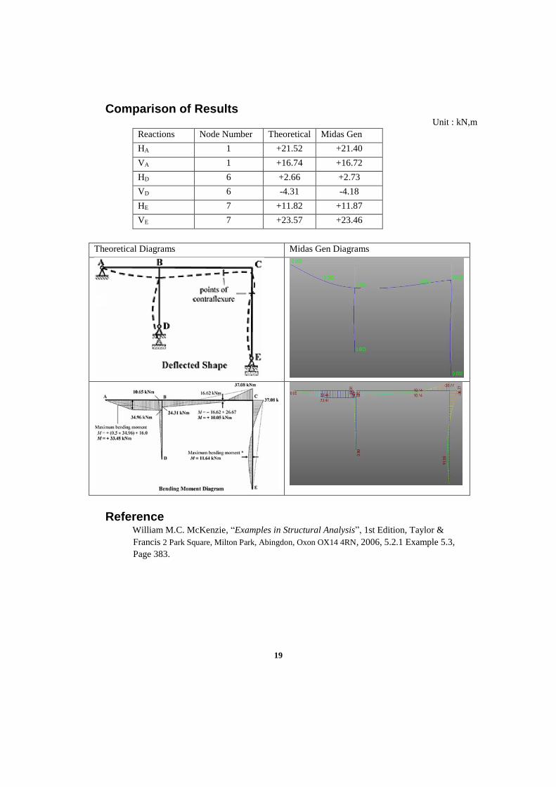
Comparison of Results Unit : kN,m

Reactions Node Number Theoretical Midas Gen

HA 1 +21.52 +21.40

VA 1 +16.74 +16.72

HD 6 +2.66 +2.73

VD 6 -4.31 -4.18

HE 7 +11.82 +11.87

VE 7 +23.57 +23.46

Theoretical Diagrams Midas Gen Diagrams

Reference William M.C. McKenzie, “Examples in Structural Analysis”, 1st Edition, Taylor &

Francis 2 Park Square, Milton Park, Abingdon, Oxon OX14 4RN, 2006, 5.2.1 Example 5.3,

Page 383.