Static and dynamic analysis of collapse behaviour of … Methods in Applied Mechanics and...

Computer Methods in Applied Mechanics and Engineering 91 (1991) 1365-1378 North-Holland

Static and dynamic analysis of collapse behaviour of steel structures

Akira Wada The Research Laboratory of Engineering Materials. Tokyo Institute of Technology, Nagatsuta.

Midori-ku, Yokohama 227, Japan

Hideyuki Kubota Building Engineering Department. Nippon Telegraph and Telephone Corporation, Midori-cho 3-9- 11,

Musashino-shi. Tokyo 180, Japan

Received 30 October 1990 Revised manuscript received 10 February 1991

1. Introduction

With the progress of structural engineering and technology, architects have desired to implement more complicated and flexible design, especially for large span structures and high-rise buildings. In these structures, it is almost impossible to ensure safety by the experiments with their actual size models. The structural analysis should be performed to check the safety. Furthermore, to confirm the true safety, not only linear elastic behavior but also nonlinear behavior of a structure is required to be carefully pursued until its collapse.

Analytic solutions in explicit form based on the theory of structural mechanics have the advantage that they can figure out the action of a structure in both quality and quantity. However, the behavior of real complicated buildings with nonlinear characteristics still cannot be expressed in explicit form. Therefore, numerical analysis using computers becomes effective and critically important.

This paper presents the computer program to pursue nonlinear behavior of steel structures until collapse state statically and dynamically, and it shows two results of example analyses. The program presented in this paper is specially designed to use the vector-processing function of super computer quite effectively. ETA10 (1.2 GFLOPS/8 CPU, 2 GB /8 CPU) and CRAY- 2 (1.9GFLOPS/4CPU, 2GB/4CPU) are used in Examples 1 and 2, respectively.

2. Modelling and assumptions

2.1. Degrees of freedom at nodal points

In this analysis, the displacement vector x and the force vector f respectively consist of seven components at each nodal point as follows:

00457825/91/$03.50 0 1991 Elsevier Science Publishers B.V. All rights reserved

1366 A. Wada. H. Kubota. Static and dynamic analysis of collapse behaviour

where the first three components indicate local element coordinates x, y, z and the following three components indicate rotations about the x, y, z-axis, respectively, the last component is used to express the warping of section. The warping of section is neglected at closed sections. Hereafter, we simply use ‘rotational degrees of freedom’ for both rotational and warping degrees of freedom.

2.2. Member

We treat each member as a beam. Each member is divided into short beam elements in axial direction as shown in Fig. 1. The deformation, strain and stress are to be calculated for each element.

2.3. Element

At each element, the following items are to be considered: - The deformation in axial direction (x-axis in local element coordinates). - The bending deformation in bi-axial directions ( y and z-axes in local element coordinates). -The torsional deformation about axis of member including St. Venant torque. - The sectional warping deformation.

We neglect the deformation caused by shear stress which will occur simultaneously relating to the bending and warping deformation. Au: Incremental displacement in x direction (parallel to the member of axis) is expressed

by a first-degree polynomial of x. Au, Aw: Incremental displacements in y, z direction (orthogonal to the member of axis) are

expressed by third degree polynomials of x. A4: Incremental torsion is expressed by a third-degree polynomial of x. As an exception,

incremental torsion of a closed section is expressed by a first degree polynomial of x. Considering large displacement, the incremental strain in the x direction at an arbitrary

point in an element can be expressed by the following equations. In these equations, w(y, z) represents the warping function.

AE~ = A&,, + A&.,? , (3)

Fig. 1. Member and elements.

A. Wada, H. Kubota, Static and dynamic analysis of collapse behaviour 1367

Fig. 2. Sectional unit areas.

where A&:,, can be expressed by a first degree polynomial of incremental displacements, A&.,

can be expressed by a second degree polynomial of them, and dA+ /dx represents the average torsional rate of an element.

We define 1 as the length of an element. According to the Gauss-Legendre quadrature, we subdivide the section into more than thirty small sectional unit areas as shown in Fig. 2 at the point of (l/2 ? 1/(2fl))1. The stress-strain relationship in each unit area is to be pursued.

2.4. Section

A section is assumed to maintain plane for any bi-axial bending deformation in either elastic or plastic state. The warping function w( y, z) corresponding to sectional configuration can be used in either elastic or plastic state without any change.

2.5. Material

The yield of element material is estimated relating to the axial strain E, and the axial stress O-,, the influence of the shear stress is neglected. The relationship between E, and a, is regarded as bi-linear. All elements are always assumed to be elastic for the St. Venant torque.

3. The static condensation of internal nodal displacements

In this analysis, when we use members such as beams and columns in which bending should be taken into account, each member is divided into ten to twenty elements in axial direction. The newly produced nodal points as the result of this division are called internal nodal points hereafter. The influence of deformation and force at any internal nodal point are limited within each member. Hence, we can eliminate degrees of freedom at these internal nodal points using substructure method. Consequently, we should treat only the degrees of freedom at both end points which come to represent the degrees of freedom of the member.

1368 A. Wada, H. Kubota, Static and dynamic analysis of collapse behaviour

These calculations include inverse matrices. To enhance the efficiency of numerical calculations, we effectively designed the program to use vector processing function which distinguishes super computers. The condensation of internal nodal degrees of freedom is implemented by the routine as shown in Appendix A. This condensation routine is executed most frequently in the structural analysis of large structures. In later mentioned examples, about eighty percent of the execute steps are used to perform this routine. This program gives full play to the vector-processing function. Furthermore, each member can be treated independently using the substructure method. Therefore, this program becomes more effective for multiprocessing super computers.

4. Mass matrix

In an architectural structure, the weight of each member is quite small as compared with the total weight of the structure or the internal force of the member. For this reason, we do not try to distribute the weight of each member over itself. We adopt the mass matrix in lumped mass form which treats the weight as a concentrated mass on the nodal point.

5. Numerical analysis methods

5.1. Dynamic analysis

We assume that inertia force and external force are not applied to rotational degrees of freedom at each nodal point, and they are only applied to translational degrees of freedom. The stiffness of a structure is assumed not to change within each time interval, from time t to t + At. By separating rotational degrees of freedom and translational degrees of freedom, the equation of motion can be expressed as follows:

where AX, AX, are the incremental displacement vectors at time t; a, a, the acceleration vectors at time t; K,, , K,,, Kzl, K,, the current stiffness matrices at time t; M the mass matrix; f, f, the internal force vectors at time t; and F the external force vector at time t; in which terms with subscript r relate to rotational degrees of freedom, and terms without r relate to translational degrees of freedom.

Eliminating AX, from (6), we obtain

(7)

Here we define K’, f' as follows:

K’ = IL2 - K2,K;,‘K,7 ,

f’ =f - KJ;,‘fr .

(8)

(9)


We obtain the equation of motion which relates to the translational degrees of freedom:

Ma,+K’Ax+f’=F. (10)

This calculation of (8) and (9) can be also executed in short time with the routine using vector-processing function of super computers as shown in Appendix A.

We calculate the response of the structure by the direct integration of (10) using Newmark’s p-parameter method. The acceleration vector at time t + At can be expressed using the velocity vector u as follows:

W + P At* K:k+~r = Ft+u -f; - K;{u, + (4 - P)a At} At. (11)

We define the apparent mass matrix M’ as

M’ = M + p At* K; . (12)

M’ of (12) must be positive definite for the unknown of (11) CY,+~( can be obtained uniquely. If M is indefinite, the kinetic energy $u’Mv becomes negative or zero. Hence M is proved to

be positive definite. Even if K: is not positive because of a broken member or for other reasons, we can determine a sufficiently small At to make Ki positive definite. Therefore the existence of (Y,,~, is confirmed, and we can proceed this analysis further.

For making a damping matrix C, at first we derive w,, the angular velocity of the first natural vibration, from initial stiffness. Then we determine h,, the damping factor of this vibration. We multiply the current stiffness matrix K’ by 2h, /w, , and we define its product as the damping matrix:

C = (2h, /o,)K’ . (13)

5.2. Static analysis

In static analysis, by setting the acceleration to be zero in (6), we obtain

By performing the same procedure as in Section 5.1, the following equation can be derived from (14):

K’Ax+f’=F. (15)

Using the step by step method, iterations are to be performed until when the accuracy at each load step is evaluated to satisfy convergent tolerance.

The convergence criterion is that the norm of unequilibrium force vector F -f’ is equal or less than the norm of external load vector F multiplied by 10P8. In structures with severe nonlinear characteristics or in unstable structures, the pursuit of structural behavior based on the theory that external force is always equal to the resistance force of the structure, will be


very difficult or even impossible to be completed. Although the constant arc method could be effective in non-linear analysis of these structures, it might be difficult for this method to treat break and sudden buckling of members.

6. Example 1. Numerical analysis of reticulated space truss

6.1. Analytical model

This example as shown in Fig. 3 treats well-known snap through problem of reticulated space truss. This problem has been studied by Hangai and Kawamata [l] and Tachibana [2] and other researchers [3-61.

All members are assumed to consist of the same material and have the same sections. In this model we treat steel members. In each member, Young’s modulus is set as E = 2.06 x 10” Pa, the sectional area is set as A = 4.77 x lo-’ m’. Each member is to be always elastic and the buckling of member is out of consideration.

6.2. Boundary conditions

Pin joint is used for all connections of members. At the nodal points of the surrounding boundary (indicated by . in Fig. 3), the translational displacements are to be restricted, and the rotational ones are to be free.

6.3. Static analysis and its result

In static analysis, by controlling the displacement of central point, the external load is applied to the central point 1 of the reticulated space truss. A vertical downward direction is defined to be positive in load and displacement. We show its result with the dynamic analysis result in Fig. 7. As indicated in this figure, this calculation could not be proceeded because the stiffness matrix becomes singular at point A.

25 25

Fig. 3. Reticulated space truss (unit: m).


6.4. Dynamic analysis and its result

2.82 x lo4 kg is put on the central point (loading point) as its weight, 2.59 x lo2 kg is put on other nodal points as their weigths, respectively. The number of all degrees of freedom turned out to be 21. We figure out that the first natural period is 0.354 set, the second natural period is 0.0513 set and the 21th natural period is 0.00256 sec.

The external force F is applied to the nodal point 1 in downward vertical direction. We change F depending on time and the maximum value is set to be 150 X 1O-3 EA as shown in Fig. 4. At time 6 set, we make F get back to 0, after this instant, we let free vibration occur.

The time interval for integration is set to be 0.001 sec. The damping factor is set to be 3%. Figure 5 shows the time history of the central nodal point 1 in the vertical displacement.

This structure reaches the turning shape at point a. When the load becomes 0, free vibration whose neutral shape is the turning shape begins to occur.

Figure 6 indicates the time history of the summation of vertical reaction forces of fixed nodal points. We find the sharp fluctuations in reaction force and drastic movements, right after the structure reaches its turning shape.

Figure 7 represents the relationship between internal force and vertical displacement at nodal point 1. The results of dynamic analysis and static analysis almost coincide until point b. After point b, the structure begins to proceed its deformation by itself. We can recognize that snap through phenomenons occur suddenly. Thereafter, between point c and point d, the vibration of this structure is damped down to the turning point f. The curve between points c and d can be considered to be the same as the curve of the force-displacement relationship when the upward external force is applied to this original structure.

The existence of singular point makes static analysis impossible to be proceeded further. In this dynamic analysis the analysis can be completed, considering the fidelity of the structural response motion.

Super computer ETA10 was used in this example. The CPU time of one integration step in this dynamic analysis was 0.1 set and the total CPU time was about 600 sec.

2o04

0 1 2 3 4 5 6 t[sec]

Fig. 4. Time history of external force.

20

16.432 15

10

0 0 1 2 3 4 5 6

t[secl

Fig. 5. Time history of vertical displacement of central point.

1372

500

400

3 300

r,

z 200 0

0 14 100

0

-100

r

A. Wada, H. Kubota, Static and dynamic analysis of collapse behaviour

5oo I 400

300

200

100

0

-100 0 1 2 3 4 5 6 0 5 I.0 15 20 25

t[sec] dhl

Fig. 6. Time history of summation of vertical reaction Fig. 7. Relationship between internal force and verti- forces of Fixed points. cal displacement at central points.

7. Example 2. Numerical analysis of double layer truss

7.1. Analytical model

As an application to a real structure, we perform the collapse analysis of double layer truss using steel pipes as described in Fig. 8 and Table 1. Dynamic and static analysis is executed on the condition that each joint is rigidly connected. The experiment with its actual size model was already carried out.

7.2. Boundary conditions

The boundary conditions of this analysis are -The points indicated as l in Fig. 8 are supported in vertical direction. -The points indicated a are supported in horizontal direction.

7.3. Static analysis and its result

In static analysis, by controlling the displacement, the downward external load is applied to four intersection points of central lower chords. Vertical downward direction is defined to be positive in load and displacement. Figure 9 shows the relationship between the vertical displacement of the central point and total load. Figure 9 also indicates the result of dynamic analysis and experiment comparatively.

Figure 10 represents the relationship between the axial forces of several members and the vertical displacement of the central point.

7.4. Dynamic analysis and its result

Each nodal mass is assumed to consist only of the weights of members which are attached to this nodal point. In other words, the weight of each member is distributed equally to both ends of the member. The external load is equally applied to four intersection points of central


Fig. 8. Double layer truss (unit: cm).

lower chords. The load is increased at the certain fixed rate. About the double of the maximum strength of structure obtained in static analysis is set to be applied to the structure after five seconds.

The number of all degrees of freedom turned out to be 87. We figure out that the first natural period is 0.0436 set, the second natural period is 0.0372 set and the 87th natural period is 0.00168 sec.

The time interval for integration is set to be 0.001 sec. Figure 11 shows the time history of vertical displacement of the central point. Figure 12

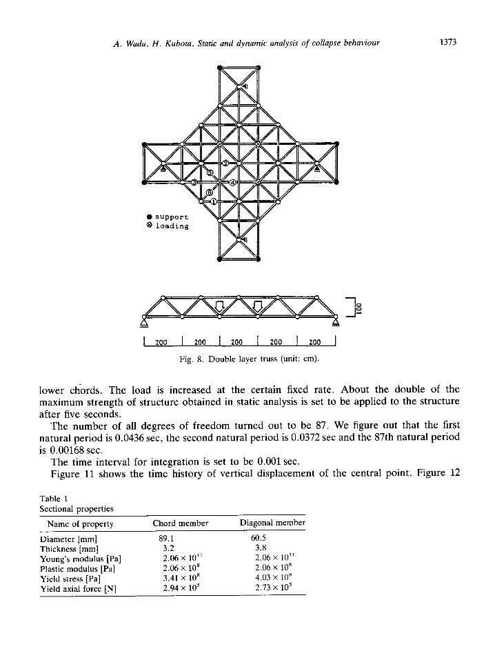
Table 1 Sectional properties

Name of property

Diameter [mm] Thickness [mm] Young’s modulus [Pa] Plastic modulus [Pa] Yield stress [Pa] Yield axial force [NJ

Chord member

89.1 3.2 2.06 x 10” 2.06 x lo8 3.41 x 10” 2.94 x lo5

Diagonal member

60.5 3.8 2.06 x 10” 2.06 x 10’ 4.03 x lo8 2.73 x 10’


dynamic analysis

experimental result-

I

0 0.05 .1 d[ml

Fig. 9. Relationship between summation of reaction forces and vertical displacement of central point.

.1

0.08

0.06

7 z

0.04

0.02

0 2.0

t[secl

Fig. 11. Time history of vertical displacement of cen- Fig. 12. Time history of summation of reaction forces tral point in dynamic analysis. of supporting points in dynamic analysis.

4

2

z c ," z

0

r(

Lk

-2

-4

_,:.- '.-element 6 _~. _-.-

_... _ _ _ _-I ‘_ - - _ _

- _ _ - eiement 3

'. '1

'\ _--- '----e-i;!ent 2

+

0 0.02 0.04 0.06 d[ml

Fig. 10. Relationship between axial forces of members and vertical displacement of central point in static analysis.

2.0 t[sec]

indicates the time history of the summation of vertical reaction forces of supporting nodal points. Figure 9 represents the relationship between the summation of the reaction forces and the vertical displacement of the central point.

In the reaction force, the experimental result is smaller than the analytical result and the reason for this is as follows. In an experiment, members are tapered off to points and their ends are jointed with bolts. On the other hand, the analysis is performed on the assumption that members have even diameter and are jointed rigidly.

The curve in Fig. 10 is bending sharply at point a. This is caused by the plastic buckling of central top chords. In the result of dynamic analysis, the deformation increases dramatically right after the buckling. During this period, the bearing capacity increases very little.

Figure 13 indicates the displacement of the central point and the axial forces of several members. Comparing Figs. 10 and 13, almost the same results are found until the buckling


4 , I 1 I

f . . element

__.. _...

__.. element __a_

__._ _ _ - -, _/ _~.' _- _.

~... _ _ - ._-_ __-_ element

_ -

‘\ ‘.

‘\ ‘. A/’ ./

2, element

4

6_

3

5

-4 ’ 0 0.02 0.04 0.06

d[ml

Fig. 13. Relationship between axial forces of members and displacement of central points in dynamic analysis.

point in both static analysis and dynamic analysis. But after buckling, dynamic analysis is under the influence of inertia force at nodal points. Consequently, we can find slight differences between them.

7.5. Advantage of static condensation in calculation time

After condensation, total matrix of this model has 180 unknowns and its half bandwidth is 64. Using a super computer (CRAY-2), it does not even take 0.1 second to solve this equation. On the other hand it takes much more time to eliminate internal nodal points. But the program is effectively designed to use vector processing function. It actually takes only 5 seconds to assemble stiffness matrix of 92 members and condense the internal displacements. If we do not perform condensation, the number of unknowns shall be 7700 and its half-band width shall be about 1300. About fifty or sixty seconds would be necessary to execute each incremental calculation. Accordingly, the static condensation of internal nodal displacements is found to be really useful in shortening calculation time.

8. Conclusion

In static analysis theory, the response of the structure subjected to an external force is considered as the change of static equilibrium conditions which can be expressed with three fundamental equations. These equations are of material consistence, the equilibrium of stress and external force, and the displacement compatibility.

While a structure is in a stable condition, the deformation has a one-to-one correspondence to its external force. The deformation and strain and stress can be derived from this relationship, and these data are very useful to grasp mechanical action of the structure.

After the structure comes in an unstable condition, the analysis could be based on the equilibrium of static external force and resistance of the structure. Actually many studies of static analysis for unstable structures have been presented. But when the buckling or the


breakage brings drastic change to the character of a structure, a proper solution is hardly obtained from these static analyses.

When we face up to real phenomena, it is just obvious that a structure has its own weight, and the sharp structural deformation whose speed cannot be neglected actually causes acceleration and inertia force. Therefore, dynamic analysis is reasonable for unstable structures. It is also efficient in numerical analysis, because we can solve an unstable equation more easily with an inertia term.

Although dynamic analysis has many advantages like this, it has on the other hand the weak point of requiring enormous calculation. The duration time of this analysis should be over several times of the longest natural period of the structure, otherwise this analysis might be strongly affected by natural vibration of the structure. Additionally, from the theory of numerical integration, the integral time interval should be less than the shortest natural period, otherwise a divergence phenomenon might occur. Hence iterations should be executed for several thousands or even several ten thousands time intervals in nonlinear dynamic analysis.

Based on these considerations we tried to use the power of super computers which have been innovated remarkably in recent years. In reticulated space truss treated in this paper, we finally pursued the structural behavior to reversed shape which cannot be figured out by static analyses. In the example of the double layer truss, we show that this analysis can well be applied to a practical structure.

The nature is the continuum in space and continuous phenomena in time. A structure does not have to be divided into discrete elements. The nature does not request any time interval which is required by numerical analysis, and loading time can be lengthened without limitation. In other words, the nature iterates integration with infinitesimal time interval, for infinite times.

Accordingly, it is very difficult to express natural phenomena with high fidelity using current computers. By computers have been making dramatic progress in their ability day by day. We believe this analysis method could be established in the near future.

Acknowledgment

We appreciate the help of Mrs. Masako Yoneda, in making the English version of the paper.

Appendix A

We show the routine of static condensation in Fig. 14. The programing language is Fortran77. The meaning of each argument is explained in Table 2.

In the most frequently executed loop 190, if we use -a(j) k) /a(k, k) instead of wk(j), input /output matrix a(i, j) shall be double used in calculation. Hence a(i, j) shall be assigned to different addresses. When a variable (matrix) does not have a unique address, the vector processing function does not work well. Therefore we add wkfj) as work area for the efficient use of vector-processing function of super computers.


1 subroutine stcnd (a ,vk ,n ,f ,

L $ ke 1

4* 5*

! dimension a dimension f

8 dimension uk ii j" )

9* 10 do 11 12 13 14 15 16 170 17 *

:: *

z: 22 * 23

2': 190

;: 200

E * 30 z: 220 *

33

230 k=l,ke pv = a(k,k) if(pv.eq.O.O) pv=l.O at = 1.0 / pv do 170 j=k,n

uk( j> =-a(j,k) * at cant inue

fk =-f(k) * at

do 200 i=l,n aik = a(k,i)

do 190 j=k+l,n a(j,i) = a(j,i) + uk(j) * aik

continue f(i) = f(i) + fk * aik

continue

do 220 j=k+l,n a(j,k) = uk(j)

cant inue

f(k) = fk -1~ :z *

230 conr;lnue

36 return 37 end

Fig. 14. Routine of static condensation of internal nodal displacements.

Table 2 Argument

Variable input /output explanation

a(n, n) input

output

input

output

of eq. (6)

. -K,,‘K

[. I2

K’ 1

n ke

wk(n)

input input

number of all unknowns of a member number of unknowns to be eliminated work area

1378 A. Wada, H. Kubota. Static and dynamic analysis of collapse behaviour

References

[l] H. Hangai and S. Kawamata, Nonlinear analysis of 3-D truss (in Japanese), Proc. JSCA Symposium of Structural Analysis with Matrix, Vol. 5 (1971) 237-244.

[2] E. Tachibana, On application of the quasi-Newton method for structural analysis including the dynamic snap-through problem, Proc. IASS Symposium on Membrane Structures and Space Frames, Vol. 3 (1986) 129-136.

[3] F.W. Williams, An approach to the nonlinear behaviour of members of a rigid jointed plane framework with finite deflections, Quart. J. Mech. App. Math. 14 (4) (1964) 451-469.

[4] O.C. Zienkiewicz et al.. Geometrically nonlinear finite element analysis of beams, frames, arches and axosymmetric shells, Comput. & Structures 7 (1977) 725-735.

[5] D. Karamanlidis et al., Large deflection finite element analysis of pre- and post-critical response of thin elastic frames, Nonlinear FE Analys. in Structural Mechanics (Springer, New York, 1981) 217-235.

[6] K. Kondoh et al., An explicit expression for the tangent-stiffness of a finitely deformed 3-D beam and its use in the analysis of space frames, Comput. & Structures 24 (2) (1986) 253-271.

[7] K. Shirotani et al., A study of steel space truss frame - Part 2 experiment of double layer NS truss frame (in Japanese), Research of Iron Manufacture, No. 313 (1984) 84-92.

Static and dynamic analysis of collapse behaviour of … Methods in Applied Mechanics and...

Documents

Transcript of Static and dynamic analysis of collapse behaviour of … Methods in Applied Mechanics and...