
Static Analysis of Stochastic Process Algebras - … · Summary The Performance Evaluation Process...
137
Static Analysis of Stochastic Process Algebras Fan Yang Kongens Lyngby 2007 IMM-MSC-2007-9
Transcript of Static Analysis of Stochastic Process Algebras - … · Summary The Performance Evaluation Process...

Static Analysis of StochasticProcess Algebras
Fan Yang
Kongens Lyngby 2007IMM-MSC-2007-9

2

Summary
The Performance Evaluation Process Algebra, PEPA, is introduced by JaneHillston as a stochastic process algebra for modelling distributed systems andespecially suitable for performance evaluation. A range of tools has alreadybeen developed that apply this algebra to various application areas for differentpurposes.
In this thesis, we present a static analysis more precisely approximating thecontrol structure of processes expressed in PEPA. The analysis technique weadopted is Data Flow Analysis which is often associated with the efficient im-plementation of classical imperative programming languages. We begin theanalysis by defining an appropriate transfer function, then with the classicalworklist algorithm we construct a finite automaton that captures all possibleinteractions among processes. With the help of the novel methodology of anno-tating label and layer to the PEPA program, the approximating result is veryprecise.
Later we try to accelerate the analysis by two approaches, and develop algo-rithms for validating the deadlock property of the PEPA program. In addition,the thesis comes out with a tool that fully implements the analyses and it couldbe used to verify the deadlock property of the PEPA programs in a certain scale.
Keywords: PEPA, Date Flow Analysis, Control Structure, Finite Automaton,Deadlock, Static Analysis, Stochastic Process Algebra.

ii
Preface
This thesis is the result of my work at the Informatics and Mathematical Mod-elling department of Technical University of Denmark, for obtaining a M.Scdegree of Computer System Engineering. It corresponds to 30 ECTs points andis carried out in the period through 1st August 2006 to 31st January 2007, underthe supervision of Professor Hanne Riis Nielson.
Lyngby, January 2007
Fan Yang

iv

Acknowledgements
First of all, I would like to thank Hanne Riis Nielson, my supervisor, for herexcellent guidance through out the whole project. I could always get a lot ofinspiration from talking with her, which makes the project going pretty smoothand efficient.
Then I would like to thank our project partner Stephen Gilmore. He providesme a series of excellent jobshop examples which show preciousness at the laststage of the project. I would also like to thank Raghav Karol, who gave mevery useful suggestions on Latex documentation and always try to share hisknowledge with me. Then I would like to thank the people at the LanguageBased Technology group who make me a pleasant stay when I work on thethesis.
Lastly, I would like to give special thanks to my beloved girlfriend Ziyan Feng,for her emotional support and proofreading my thesis several times. Of course,I always feel very grateful for the support from my parents, and thank them fortrying to make my life easier when I study abroad.

vi
Contents
Summary i
Preface iii
Acknowledgements v
1 Introduction 1
1.1 Theoretical Background . . . . . . . . . . . . . . . . . . . . . . . 2
1.2 Our work . . . . . . . . . . . . . . . . . . . . . . . . . . . . . . . 3
1.3 Thesis Organization . . . . . . . . . . . . . . . . . . . . . . . . . 4
2 Performance Evaluation Process Algebra 7
2.1 Syntax . . . . . . . . . . . . . . . . . . . . . . . . . . . . . . . . . 7
2.2 Semantics . . . . . . . . . . . . . . . . . . . . . . . . . . . . . . . 9
2.3 The introduction of Label and Layer to PEPA . . . . . . . . . . 11

viii CONTENTS
3 Exposed Actions 15
3.1 Extended Multiset M and Extra Extended Multiset Mex . . . . . 15
3.2 Calculating Exposed Actions . . . . . . . . . . . . . . . . . . . . 19
3.3 Termination . . . . . . . . . . . . . . . . . . . . . . . . . . . . . . 21
4 Transfer Functions 23
4.1 Extended Multimap T and Extra Extended Multimap Tex . . . . 24
4.2 Generated Actions . . . . . . . . . . . . . . . . . . . . . . . . . . 24
4.3 Killed Actions . . . . . . . . . . . . . . . . . . . . . . . . . . . . . 29
4.4 The Transfer Function . . . . . . . . . . . . . . . . . . . . . . . . 36
5 Constructing the Automaton 41
5.1 The worklist algorithm . . . . . . . . . . . . . . . . . . . . . . . . 43
5.2 The procedure update . . . . . . . . . . . . . . . . . . . . . . . . 44
5.3 The computation of enabled exposed actions . . . . . . . . . . . 52
5.4 Correctness result . . . . . . . . . . . . . . . . . . . . . . . . . . . 65
5.5 Termination of the worklist Algorithm . . . . . . . . . . . . . . . 67
6 Accelerate the Analysis 71
6.1 Method 1 . . . . . . . . . . . . . . . . . . . . . . . . . . . . . . . 72
6.2 Method 2 . . . . . . . . . . . . . . . . . . . . . . . . . . . . . . . 75
6.3 Three Approaches of Analysis on Two Examples . . . . . . . . . 81
6.4 Discussion of method1 and method2 . . . . . . . . . . . . . . . . 85

CONTENTS ix
7 Deadlock Verification 89
7.1 Deadlock of PEPA . . . . . . . . . . . . . . . . . . . . . . . . . . 89
7.2 Detect the Deadlock by Our Analysis . . . . . . . . . . . . . . . . 90
7.3 Detect the Deadlock of Jobshop Examples . . . . . . . . . . . . . 92
8 Conclusion 99
8.1 Achievement . . . . . . . . . . . . . . . . . . . . . . . . . . . . . 99
8.2 Limitation . . . . . . . . . . . . . . . . . . . . . . . . . . . . . . . 100
8.3 Future Work . . . . . . . . . . . . . . . . . . . . . . . . . . . . . 100
A The Syntax of Jobshop 4 - 11 103
B Design and Demonstration of the Tool 111
B.1 The Parser . . . . . . . . . . . . . . . . . . . . . . . . . . . . . . 113
B.2 The Analyzer . . . . . . . . . . . . . . . . . . . . . . . . . . . . . 113
B.3 A Guide for Using the Tool through an Example . . . . . . . . . 115
B.4 Analysis Results . . . . . . . . . . . . . . . . . . . . . . . . . . . 116
B.5 Source Code . . . . . . . . . . . . . . . . . . . . . . . . . . . . . . 122

x CONTENTS

Chapter 1
Introduction
In computer science, the process calculi (or process algebras) are a diversefamily of related approaches to formally modelling concurrent systems. Theyprovide a tool for the high-level description of interactions, communications,and synchronizations between a collection of independent processes [35]. Themost famous ones include: Communicating Sequential Processes(CSP)[24] ,Cal-culus of Communicating Systems (CCS) [26] and Algebra of CommunicatingProcesses(ACP)[9].
Among them there is a branch of process algebras extended with probabilisticor stochastic information, which are usually named stochastic process algebras(SPAs). For example, in CSP tradition, there is Timed CSP [20], in CCS tradi-tion, there is PEPA [22], and prACP−I [8] is in ACP tradition. The SPAs havegained acceptance as one of the techniques available for performance analy-sis. For example, in large computer and communication systems, they could beused to model the system and predict the behavior of a system with respect todynamic properties such as throughput and response time[23].
However, the system modelling with SPAs always inherits the process algebras’sconcurrent essentials and behaves in a complex way. When dynamically execut-ing the system, we sometimes need to be ensured that there must not arise anyabnormal event. For example, the system shouldn’t terminate unexpectedly(nodeadlock). Furthermore, sometimes even though we are notified that the sys-

2 Introduction
tem might go into the deadlock states, we are not satisfied. We are also curiousin which steps might we reach those states, because this information would bevery useful for understanding the cause of the abnormity and then help peopleto revise the system to avoid deadlock.
In this thesis, we are going to develop a static analysis for one kind of SPAs:Performance Evaluation Process Algebra (PEPA) [22], aiming at answering thefollowing two questions for the system modelled with PEPA:
• Does the system potentially have chance to go into the deadlock states?
• If there exist deadlock states, how does the system behave before reachingthose states?
In the following subsections, first we will introduce the theoretical backgroundof our work. Then we give a short description of the real work we accomplished.In the last of this chapter we will outline the structure of the thesis.
1.1 Theoretical Background
1.1.1 Related Works
In recently years, there are several methods of applying static analysis techniquesto highly concurrent languages and a variety of process algebras. For processalgebras, the works are mainly based on three approaches:
• One line of work is to adapt Type Systems from the functional and object-oriented languages to express meaningful properties of the process alge-bras(e.g. [27, 34]).
• Another line of work is based on Control Flow Analysis. The process alge-bras that have been extensively researched are: pi-calculus [10], variantsof mobile ambients(e.g. [12, 29]) and process algebras for cryptographicprotocols such as Lysa [11].
• The last line of work just emerges recently, and it uses the classical ap-proach – Data Flow Analysis to focus on analyzing transitions instead ofconfigurations of the models (Configurations are the main concern of theprevious two approaches). The process algebras that has already beendone includes CCS [15, 16].

1.2 Our work 3
Our work adopts the last approach, because its special feature of transitiontracking would help us easily answer not only the first question (verify deadlockproperty) but also the second question mentioned above (find paths leading todeadlock states). And the work in [15, 16] inspires our own work quite a lot.
1.1.2 Analysis Techniques
Our work is based on the category of program analysis, in particular the DataFlow Analysis, which will be introduced briefly as follows.
Program analysis offers static compile-time techniques for predicting safe andcomputable approximations to the set of values or behaviors arising dynamicallyat run-time when executing a program on a computer[28].
The safe here means that analysis is based on formal semantics (Our job isbased on the semantics of PEPA). The approximations are usually divided intothree classes:(a)Over-approximation captures the entire behavior of the pro-gram. (b)Under-approximation captures a subset of all possible behavior of theprogram in reality.(c)Undecidable-approximation can’t decide whether the theapproximation behaviors belong to the program or not. In our work, we willuse both (a) and (b) approaches for approximation.
The Data Flow Analysis is among four classical program analysis approaches,which are Data Flow Analysis, Constraint Based Analysis, Abstract Interpreta-tion and Type and Effect Systems. In Data Flow Analysis, it is customary tothink of a program (written in traditional programming language) as a graph:the nodes are basic blocks and the edges describe how control might pass fromone basic block to another. The transfer functions associated with basic blocksare often specified as Bitvector Frameworks or more general as Monotone Frame-works. The transfer functions in Bitvector Frameworks will always remove in-formation no longer appropriate, and at the same time generate appropriateinformation to the basic blocks which will form new basic block.
1.2 Our work
Our work is based on the Data Flow Analysis. We build a graph (actuallywe generate an automaton from the program while the graph is the graphicalrepresentation of the automaton) for the program written in PEPA, which couldcapture the control structure of the program. And this automaton could be used

4 Introduction
to verify deadlock property and illustrate paths leading to deadlock states.
Concretely, we first specify the kill and gen function based on the semantics ofthe PEPA and make our own transfer function. For the safe approximation, weperform under-approximation for the kill function and the over-approximationfor the gen function: it is always safe to kill less information and gen moreinformation than the exact information. We shall see that the labels and lay-ers of individual actions(labels and layers are annotation to the PEPA programwhile action is a term in PEPA, please refer to chapter 2 in details) will corre-spond to the basic blocks of Data Flow analysis and there is a need to introducetwo domains : extended multisets and extra extended multisets to replace theBitvectors for these functions.
Later we will use worklist algorithm to construct a finite control flow graph(automaton) for PEPA process: the nodes describe the exposed actions(will beintroduced in chapter 3) for the various configuration (state) that may arisedynamically during the execution; the edges describe the interactions of ac-tions(transitions) that tell how one configuration evolves to another configu-ration. For the termination of the algorithm, we adopt a suitable granularityfunction and the widening operator.
Lastly, to improve the analysis efficiency, we develop two methods which couldsignificantly speed up the analysis when some information is ignored.
After developing these analyses, we utilize them first to verify several smallprograms and then study the deadlock property of a series of larger programs:variants of Milner’s process for a jobshop [31].
1.3 Thesis Organization
Chapter 2 introduces the syntax of PEPA as well as its semantics. In addition,layers and labels are equipped to PEPA.
Chapter 3 first introduces the concept of exposed actions for PEPA program andtwo domains: extend multiset and extra extend multiset. Later two functionsEs
? and Ep? are developed to compute the information for initialization worklist
algorithm.
Chapter 4 describes the development of function kill(Ks?,K
p?), gen(Gs
?,Gp?) and
finally the transfer function which will be invoked in the worklist algorithm.The domain extend multimap and extra extend multimap are introduced.

1.3 Thesis Organization 5
Chapter 5 describes the constructing of the automaton by worklist algorithm.Some auxiliary functions are developed to cooperate with the worklist algorithm,such as update, enabled, Ys
? , Yp? etc.
Chapter 6 discusses two methods for increasing the analysis speed (constructingthe automaton) on the condition that the structure of PEPA program meetsome requirements.
Chapter 7 shows how to use the analysis developed in the previous chaptersto verify the deadlock property of PEPA programs and how to find the pathsleading to each deadlock state.
Chapter 8 concludes the thesis and points out some future work.

6 Introduction
Chapter 2
Performance EvaluationProcess Algebra
In this chapter we shall first introduce the syntax of PEPA programs and thenreview the semantics as presented in [22]. Lastly we will equip PEPA withlabels and layers that would be helpful for the analysis developed later.
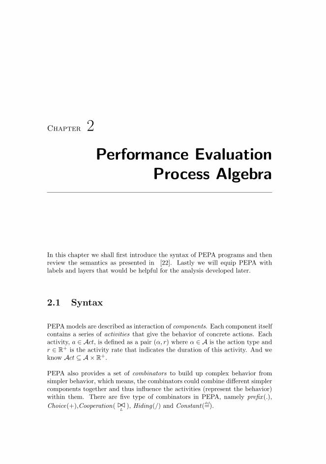
2.1 Syntax
PEPA models are described as interaction of components. Each component itselfcontains a series of activities that give the behavior of concrete actions. Eachactivity, a ∈ Act, is defined as a pair (α, r) where α ∈ A is the action type andr ∈ R+ is the activity rate that indicates the duration of this activity. And weknow Act ⊆ A× R+.
PEPA also provides a set of combinators to build up complex behavior fromsimpler behavior, which means, the combinators could combine different simplercomponents together and thus influence the activities (represent the behavior)within them. There are five type of combinators in PEPA, namely prefix (.),Choice(+),Cooperation( ��
L), Hiding(/) and Constant(def=).

8 Performance Evaluation Process Algebra
Prefix: (α, r).S: Prefix is the basic mechanism by which the behaviors of com-ponents are constructed. It means after the component has carried outactivity (α, r), it will behave as component S.
Choice: S1 + S2: This combinator represents a system which may behave ei-ther as component S1 or as S2. S1 +S2 enables all the current activities ofS1 and all the current activities of S2. The first activity to complete distin-guishes one out of the two components, S1 or S2 and the other componentof the choice is then discarded.
Cooperation: P1 ��L
P2: This combinator describes the synchronization of theP1 and P2 over the activities in the cooperation set L. The componentsmay proceed independently with activities whose types do not belong tothis set. In contrast, the components should cooperate with the othercomponents if the types of their activities (to be executed) both fall intothis set.
Hiding: P/L: It behaves as P except that any activities of types within the setL are hidden, meaning that their type is not witnessed upon completion.A hidden activity is witnessed only by its delay and the unknown type τ ,and it can’t be carried out in cooperation with any other component.
Constant: Cdef= S or S
def= P : Constant are components whose meaning is givenby a defining equation such as C
def= S or Sdef= P which gives the constant C
the behavior of the component S or S given the behavior of P respectively.This is how we assign names to components (behaviors).
The syntax is formally defined by means of the following grammar.
S ::= (α, r).S | S1 + S2 | CP ::= P1 ��
LP2 | P/L | S
where S denotes a sequential component and P denotes a model component.A sequential component could be formed by sequential combinators that is ei-ther prefix, choice or constant C where C stands for sequential component. Amodel component could be formed by model combinators that is either cooper-ation, hiding or constant S where S stands for sequential component or modelcomponent.
We shall be interested in programs of the form
let C1 , S1; · · · ;Ck , Sk︸ ︷︷ ︸Sequential Component definition
in P0︸︷︷︸Model Component definition
where the Sequential processes (sequential components) named C1, · · · , Ck(∈PN) are mutually recursively defined and may be used in the main model

2.2 Semantics 9
process P0 (P0 is formed by model components connected with model combina-tors) as well as in the sequential process bodies S1, · · · , Sk. We shall require thatC1, · · · , Ck are pairwise distinct and that they are the only sequential processnames used. In turn, P0 is the main model component which is essentially de-scribed by ��
Land / combinators to join the sequential processes C1, · · · , Ck.
And these sequential processes are also called model components in model com-ponent definition.
Another thing should be mentioned here is that cooperation between severaldifferent components using differing cooperation sets may be regarded as beingbuilt up in layers. Each cooperation combining just two components whichthemselves might be composed from cooperation between components at a lowerlevel. For example:
(P1 ��L
P2) ��K
P3
In this case, the top layer could be Q1 ��K
Q2 where, at the lower level, if ≡denotes syntactic equivalence, Q1 ≡ P1 ��
LP2 and Q2 ≡ P3.
Example 2.1 Let’s transform a program written in PEPA syntax into the pro-gram with our form:
Sdef= (g, r1).(p, r2).S
Qdef= (g, r3).(h, r4).Q + (p, r5).Q
S ��{g,p}
Q
would be transformed into
let S , (g, r1).(p, r2).SQ , (g, r3).(h, r4).Q + (p, r5).Q
in S ��{g,p}
Q
Here we also give other two programs: the sequential components remain thesame as above, while the main model component are defined as (S ��
{}S) ��
{g,p}Q
and (S ��{g,p}
S) ��g,p
Q respectively. These three programs would be furthered dis-cussed in the following examples.
2.2 Semantics
Following [22] the calculus is equipped with a reduction semantics. The reduc-tion relation E →(α,r) E′ is specified in Table 2.1 and expresses that the processE in one step may evolve into the process E′.

10 Performance Evaluation Process Algebra
Prefix
(α, r).E →(α,r) E
Cooperation
E →(α,r) E′
E ��L
F →(α,r) E′ ��L
F(α /∈ L)
F →(α,r) F ′
E ��L
F →(α,r) E ��L
F ′ (α /∈ L)
E →(α,r1) E′ F →(α,r2) F ′
E ��L
F →(α,R) E′ ��L
F ′ (α ∈ L) where R =r1
rα(E)r2
rα(F )min(rα(E), rα(F ))
HidingE →(α,r) E′
E/L →(α,r) E′/L(α /∈ L)
E →(α,r) E′
E/L →(τ,r) E′/L(α ∈ L)
Choice
E →(α,r) E′
E + F →(α,r) E′
F →(α,r) F ′
E + F →(α,r) F ′
Constant
E →(α,r) E′
A →(α,r) E′ (A def= E)
Table 2.1: Operational semantics of PEPA
2.3 The introduction of Label and Layer to PEPA 11
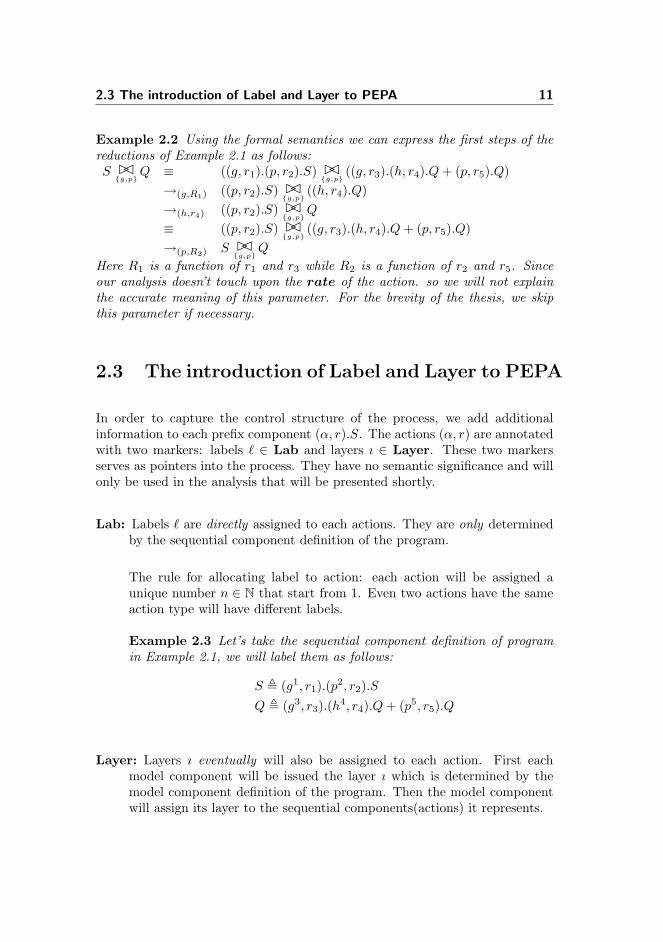
Example 2.2 Using the formal semantics we can express the first steps of thereductions of Example 2.1 as follows:S ��
{g,p}Q ≡ ((g, r1).(p, r2).S) ��
{g,p}((g, r3).(h, r4).Q + (p, r5).Q)
→(g,R1) ((p, r2).S) ��{g,p}
((h, r4).Q)→(h,r4) ((p, r2).S) ��
{g,p}Q
≡ ((p, r2).S) ��{g,p}
((g, r3).(h, r4).Q + (p, r5).Q)→(p,R2) S ��
{g,p}Q
Here R1 is a function of r1 and r3 while R2 is a function of r2 and r5. Sinceour analysis doesn’t touch upon the rate of the action. so we will not explainthe accurate meaning of this parameter. For the brevity of the thesis, we skipthis parameter if necessary.
2.3 The introduction of Label and Layer to PEPA
In order to capture the control structure of the process, we add additionalinformation to each prefix component (α, r).S. The actions (α, r) are annotatedwith two markers: labels ` ∈ Lab and layers ı ∈ Layer. These two markersserves as pointers into the process. They have no semantic significance and willonly be used in the analysis that will be presented shortly.
Lab: Labels ` are directly assigned to each actions. They are only determinedby the sequential component definition of the program.
The rule for allocating label to action: each action will be assigned aunique number n ∈ N that start from 1. Even two actions have the sameaction type will have different labels.
Example 2.3 Let’s take the sequential component definition of programin Example 2.1, we will label them as follows:
S , (g1, r1).(p2, r2).SQ , (g3, r3).(h4, r4).Q + (p5, r5).Q
Layer: Layers ı eventually will also be assigned to each action. First eachmodel component will be issued the layer ı which is determined by themodel component definition of the program. Then the model componentwill assign its layer to the sequential components(actions) it represents.

12 Performance Evaluation Process Algebra
The rule for allocating layer to model component: each model componentwill be assigned a unique vector v (represents the layer) that containselement e ∈ {0, 1}. v is composed depending on the tree structure of thecooperation combinator. e will be appended to v from the top layer tothe lower layer of the combinator tree in sequence. v has two part: thelocation that takes up the rightmost position of the vector, and the currentlayer that consists of all elements left to the rightmost element. And thelefthanded side of combinator will be assigned 0 while righthanded sidewill be assigned 1. The top layer is assumed to be assigned 0. For example:
Example 2.4 Let’s take one of the model component definition of pro-gram in Example 2.1, we will add layer to each model component as fol-lows:
( S︸︷︷︸000
��{}
S︸︷︷︸001
) ��{g,p}
Q︸︷︷︸01
or (S000 ��{}
S001) ��{g,p}
Q01
where S on the left has layer 000: its current layer is 00, and since it is onthe lefthanded side of ��
{}, its location is 0. Q has layer 01: its current
layer is 0 (the top layer), and due to the fact it is on the righthanded sideof ��
{g,p}, its location is 1.
Then we will grant layer to actions from model component. Let’s take Sfrom sequential component definition of program in Example 2.1 with layer000 as the example:
S , (g, r1)000.(p, r2)000.S
Here all actions(g and p) will be assigned their model component’s layer000.
If we annotate the syntax of the prefix component (α, r).S with two new nota-tions, eventually it will change to (α`, r)ı.S.
Example 2.5 If we take S from Example 2.1, label it as in Example 2.3 andlayer it with 000 as in Example 2.4, each action within S will be marked asfollows:
S , (g1, r1)000.(p2, r2)000.S
The above annotation doesn’t impact the significance of the semantics at all.However, to facilitate the analysis, we present two versions of semantics asfollows for different purposes.
Table 2.2 shows the semantics of the sequential component of PEPA only equippedwith label but omit layer. This is because the layer of a certain sequential com-ponent always remain the same even when it evolves to other form of sequential

2.3 The introduction of Label and Layer to PEPA 13
Sequential Component
Prefix(α`, r).S →α` S
Choice1S1 →α`1 S′1
S1 + S2 →α`1 S′1
Choice2S2 →α`2 S′2
S1 + S2 →α`2 S′2
ConstCS →α` S′
C →α` S′(C def= S)
Table 2.2: Semantics of the sequential components of PEPA equipped with label
component. The label itself is enough to clearly illustrate the effect of eachtransition among sequential components.
Table 2.3 demonstrates the semantics of PEPA equipped with both label andlayer. It contains two parts explaining exactly the syntax of PEPA introducedin Subsection 2.1.
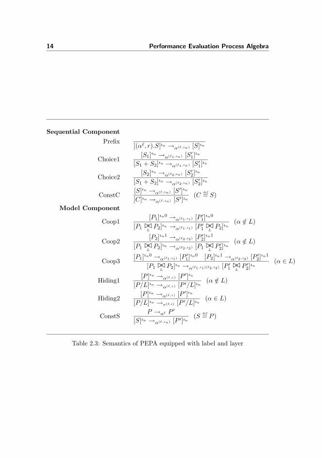
14 Performance Evaluation Process Algebra
Sequential Component
Prefix[(α`, r).S]ın →α(`,ın) [S]ın
Choice1[S1]ın →α(`1,ın) [S′1]
ın
[S1 + S2]ın →α(`1,ın) [S′1]ın
Choice2[S2]ın →α(`2,ın) [S′2]
ın
[S1 + S2]ın →α(`2,ın) [S′2]ın
ConstC[S]ın →α(`,ın) [S′]ın
[C]ın →α(`,ın) [S′]ın(C def= S)
Model Component
Coop1[P1]ın0 →α(`1,ı1) [P ′
1]ın0
[P1 ��L
P2]ın →α(`1,ı1) [P ′1��
LP2]ın
(α /∈ L)
Coop2[P2]ın1 →α(`2,ı2) [P ′
2]ın1
[P1 ��L
P2]ın →α(`2,ı2) [P1 ��L
P ′2]ın
(α /∈ L)
Coop3[P1]ın0 →α(`1,ı1) [P ′
1]ın0 [P2]ın1 →α(`2,ı2) [P ′
2]ın1
[P1 ��L
P2]ın →α(`1,ı1)(`2,ı2) [P ′1��
LP ′
2]ın(α ∈ L)
Hiding1[P ]ın →α(`,ı) [P ′]ın
[P/L]ın →α(`,ı) [P ′/L]ın(α /∈ L)
Hiding2[P ]ın →α(`,ı) [P ′]ın
[P/L]ın →τ(`,ı) [P ′/L]ın(α ∈ L)
ConstSP →α` P ′
[S]ın →α(`,ın) [P ′]ın(S def= P )
Table 2.3: Semantics of PEPA equipped with label and layer

Chapter 3
Exposed Actions
An exposed action is an action that may participate in the next interaction.For instance, the sequential component S in Example 2.1 will have action g asexposed action while Q will have both g and p as exposed actions. In either case,they will have one occurrence of each type. However, in general, a process maycontain many, even infinitely many, occurrences of the same action (identifiedby the same label and layer) and it may be the case that several of them areready to participate in the next interaction. For example:
S , (α, r).SP , S + S
Here S only has one occurrence of α as exposed action, at the same time P willhave two occurrence of the same action as exposed actions and both of themare ready for next interaction.
3.1 Extended Multiset M and Extra ExtendedMultiset Mex
To capture this in [16] the authors define an extended multiset M (the domainthat our Es
? works on, Es? will be presented in Subsection 3.2 ) and we introduce
16 Exposed Actions
it in Subsection 3.1.1, and we are going to define the extra extended multisetMex (the domain that our Ep
? works on, Ep? will be presented in Subsection 3.2)
in Subsection 3.1.2 for catering to our new scenario. In the following section 3.2,we will introduce the abstraction function Es
? and Ep? that specify an extended
multiset and extra extended multiset of the program.
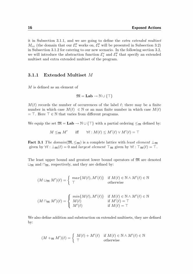
3.1.1 Extended Multiset M
M is defined as an element of
M = Lab → N ∪ {>}
M(`) records the number of occurrences of the label `; there may be a finitenumber in which case M(`) ∈ N or an max finite number in which case M(`)= >. Here > ∈ N that varies from different programs.
We equip the set M = Lab → N ∪ {>} with a partial ordering ≤M defined by:
M ≤M M ′ iff ∀` : M(`) ≤ M ′(`) ∨M ′(`) = >
Fact 3.1 The domain(M,≤M) is a complete lattice with least element ⊥M
given by ∀` : ⊥M(`) = 0 and largest element >M given by ∀` : >M(`) = >.
The least upper bound and greatest lower bound operators of M are denotedtM and uM, respectively, and they are defined by:
(M tM M ′)(`) ={
max{M(`),M ′(`)} if M(`) ∈ N ∧M ′(`) ∈ N> otherwise
(M uM M ′)(`) =
min{M(`),M ′(`)} if M(`) ∈ N ∧M ′(`) ∈ NM(`) if M ′(`) = >M ′(`) if M(`) = >
We also define addition and substraction on extended multisets, they are definedby:
(M +M M ′)(`) ={
M(`) + M ′(`) if M(`) ∈ N ∧M ′(`) ∈ N> otherwise
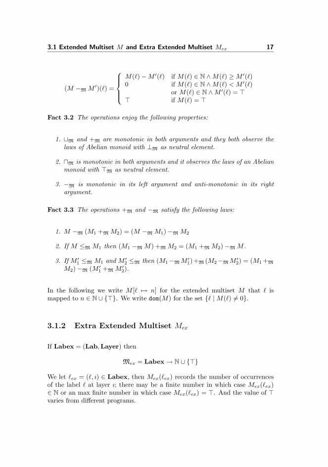
3.1 Extended Multiset M and Extra Extended Multiset Mex 17
(M −M M ′)(`) =
M(`)−M ′(`) if M(`) ∈ N ∧M(`) ≥ M ′(`)0 if M(`) ∈ N ∧M(`) < M ′(`)
or M(`) ∈ N ∧M ′(`) = >> if M(`) = >
Fact 3.2 The operations enjoy the following properties:
1. tM and +M are monotonic in both arguments and they both observe thelaws of Abelian monoid with ⊥M as neutral element.
2. uM is monotonic in both arguments and it observes the laws of an Abelianmonoid with >M as neutral element.
3. −M is monotonic in its left argument and anti-monotonic in its rightargument.
Fact 3.3 The operations +M and −M satisfy the following laws:
1. M −M (M1 +M M2) = (M −M M1)−M M2
2. If M ≤M M1 then (M1 −M M) +M M2 = (M1 +M M2)−M M .
3. If M ′1 ≤M M1 and M ′
2 ≤M then (M1−M M ′1)+M (M2−M M ′
2) = (M1 +M
M2)−M (M ′1 +M M ′
2).
In the following we write M [` 7→ n] for the extended multiset M that ` ismapped to n ∈ N ∪ {>}. We write dom(M) for the set {` | M(`) 6= 0}.
3.1.2 Extra Extended Multiset Mex
If Labex = (Lab,Layer) then
Mex = Labex → N ∪ {>}
We let `ex = (`, ı) ∈ Labex, then Mex(`ex) records the number of occurrencesof the label ` at layer ı; there may be a finite number in which case Mex(`ex)∈ N or an max finite number in which case Mex(`ex) = >. And the value of >varies from different programs.
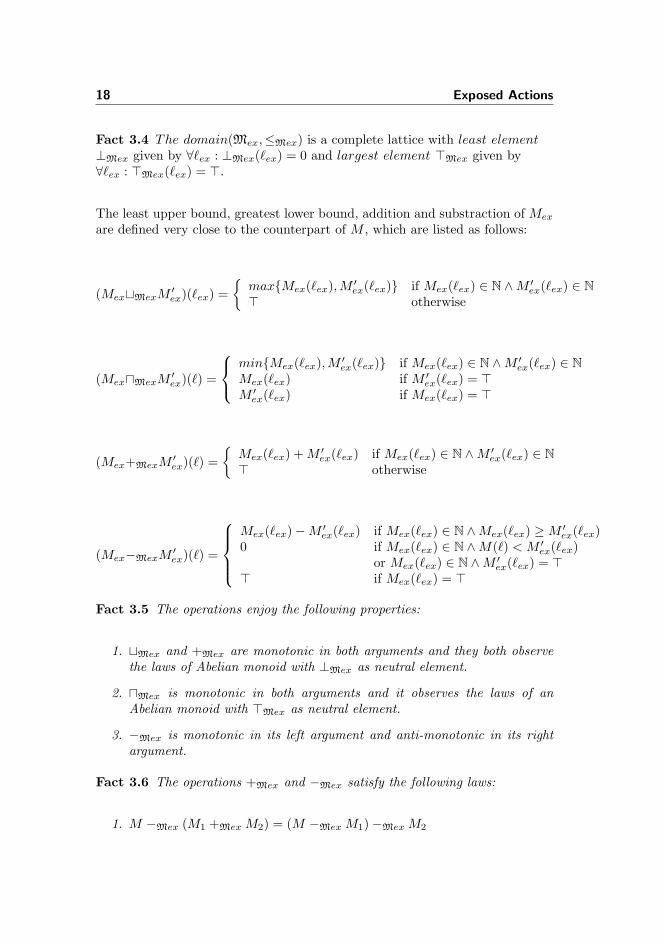
18 Exposed Actions
Fact 3.4 The domain(Mex,≤Mex) is a complete lattice with least element⊥Mex given by ∀`ex : ⊥Mex(`ex) = 0 and largest element >Mex given by∀`ex : >Mex(`ex) = >.
The least upper bound, greatest lower bound, addition and substraction of Mex
are defined very close to the counterpart of M , which are listed as follows:
(MextMexM ′ex)(`ex) =
{max{Mex(`ex),M ′
ex(`ex)} if Mex(`ex) ∈ N ∧M ′ex(`ex) ∈ N
> otherwise
(MexuMexM ′ex)(`) =
min{Mex(`ex),M ′ex(`ex)} if Mex(`ex) ∈ N ∧M ′
ex(`ex) ∈ NMex(`ex) if M ′
ex(`ex) = >M ′
ex(`ex) if Mex(`ex) = >
(Mex+MexM ′ex)(`) =
{Mex(`ex) + M ′
ex(`ex) if Mex(`ex) ∈ N ∧M ′ex(`ex) ∈ N
> otherwise
(Mex−MexM ′ex)(`) =
Mex(`ex)−M ′
ex(`ex) if Mex(`ex) ∈ N ∧Mex(`ex) ≥ M ′ex(`ex)
0 if Mex(`ex) ∈ N ∧M(`) < M ′ex(`ex)
or Mex(`ex) ∈ N ∧M ′ex(`ex) = >
> if Mex(`ex) = >
Fact 3.5 The operations enjoy the following properties:
1. tMex and +Mex are monotonic in both arguments and they both observethe laws of Abelian monoid with ⊥Mex as neutral element.
2. uMex is monotonic in both arguments and it observes the laws of anAbelian monoid with >Mex as neutral element.
3. −Mex is monotonic in its left argument and anti-monotonic in its rightargument.
Fact 3.6 The operations +Mex and −Mex satisfy the following laws:
1. M −Mex (M1 +Mex M2) = (M −Mex M1)−Mex M2

3.2 Calculating Exposed Actions 19
2. If M ≤Mex M1 then (M1 −Mex M) +Mex M2 = (M1 +Mex M2)−Mex M .
3. If M ′1 ≤Mex M1 and M ′
2 ≤Mex then (M1−MexM ′1)+Mex (M2−MexM ′
2) =(M1 +Mex M2)−Mex (M ′
1 +Mex M ′2).
We write domExlayer(Mex, ı) for the set {` | (`, ı) ∈ Labex of Mex}. We writedomEx(Mex) for the set {(`, ı) | Mex(`, ı) 6= 0}.
3.2 Calculating Exposed Actions
The information of key interest is the collection of extra extended multisets ofexposed actions of the model component processes. However, to obtain thatwe need first to get the extended multisets of exposed actions of the sequentialcomponent processes. The first step is computed by abstraction function Es
? ,and the second step by function namely Ep
? .
To motivate the definition let us first consider the combination of choice andprefix of two sequential processes (α`1
1 , r1).S1 + (α`22 , r2).S2. Here both of the
actions α1 and α2 are ready to interact but actions from S1 and S2 are not, sowe shall take:
Es[[(α`11 , r1).S1 + (α`2
2 , r2).S2]]env = ⊥M[`1 7→ 1] +M ⊥M[`2 7→ 1]
If the two labels happen to be equal (`1 = `2) the overall count will become 2since we have used the pointwise addition operator +M.
Second, if we turn to cooperation combinator, we shall have the following func-tion formula, and this time we use Ep instead:
Ep[[(α`11 , r1)00.S �� (α`2
2 , r2)01.S]] = ⊥Mex[(`1, 00) 7→ 1]+Mex⊥Mex[(`2, 01) 7→ 1]
In this case, even though `1 and `2 have the same label, According to the +Mex
operation, the overall count couldn’t become 2, because these two labels are notin the same layer.
Function E
To handle the general case we shall introduce two functions
Es : Sproc → (PN → M) → M
Ep : Pproc → Mex

20 Exposed Actions
For function Es, it takes an environment as the additional parameter whichholds the required information for the process names. The function is defined inTable 3.1 for arbitrary processes; in the case of choice and prefix, it generalizesthe clauses shown above. Turning to the clause for sequence constants we simplyconsult the environment env provided as the first argument to Es.
As shown in Table 3.1, there defines a function FE : (PN → M) → (PN →M). Since the operations involved in its definition are all monotonic (cf. Fact3.1). we have a monotonic function defined on a complete lattice (cf. Fact3.2) and Tarski’s fixed point theorem ensures that it has a fixed point whichis denoted envE in Table 3.1. Since all sequential processes are finite it followsthat FE is continuous and hence that the Kleene formulation of the fixed pointis permissible. We can now define the function
Es? : Sproc → M
Simply as Es? [[S]] = Es[[S]]envE .
For function Ep, it will always take layer ı as parameters and finally appendthe correct layer to each S sequential component. Specifically, for cooperationoperator, it will combine the result of two components by +Mex operation. Theclause for the P/L will simply ignores the hidden set L. The clause for constantmodel combinator will borrow the result get from Es
? step and use the denotationof this sequential component to compute the overall Mex. It is worth pointingout that only the label and layer pair belonging to the Mex set should be setup by each constant combinator clause.
We can now define the function
Ep? : Pproc → Mex
Simply as Ep? [[P ]] = Ep[[P ]]0.The parameter 0 takes charge of layer initialization
and is the value issued to the top layer. (cf.section 2.3).
Example 3.1 For the running example of Example 2.1 we have
Ep? [[S ��
{g,p}Q]] = [(1, 00) 7→ 1, (2, 00) 7→ 0, (3, 01) 7→ 1, (4, 01) 7→ 0,
(5, 01) 7→ 1]Ep
? [[(S ��{}
S) ��{g,p}
Q]] = [(1, 000) 7→ 1, (2, 000) 7→ 0, (1, 001) 7→ 1, (2, 001) 7→ 0,
(3, 01) 7→ 1, (4, 01) 7→ 0, (5, 01) 7→ 1]Ep
? [[(S ��{g,p}
S) ��{g,p}
Q]] = [(1, 000) 7→ 1, (2, 000) 7→ 0, (1, 001) 7→ 1, (2, 001) 7→ 0,
(3, 01) 7→ 1, (4, 01) 7→ 0, (5, 01) 7→ 1]

3.3 Termination 21
Exposed actions for let C1 , S1; · · · ;Ck , Sk in P0
Es[[(α`, r).S]]env = ⊥M[` 7→ 1]Es[[S1 + S2]]env = Es[[S1]]env +M Es[[S2]]env
Es[[C]]env = env(C)Es
? [[S]] = Es[[S]]envE
whereFE(env) = [C1 7→ Es[[S1]]env, · · · , Ck 7→ Es[[Sk]]env]and env⊥M
= [C1 7→ ⊥M, · · · , Ck 7→ ⊥M]
and envE = tj≥0FjE(env⊥M
)Ep[[P1 ��
LP2]]ı = Ep[[P1]]ı0 +Mex Ep[[P2]]ı1
Ep[[P/L]]ı = Ep[[P ]]ı
Ep[[S]]ı = let (`1 7→ n1, · · · , `n 7→ nn) = Es? [[S]]
in ⊥Mex[(`j , ı) 7→ nj ] where `j ∈ domExlayer(⊥Mex, ı)and j ∈ {1, · · · , n}
Ep? [[P ]] = Ep[[P ]]0
Table 3.1: Es and Ep function
We could see that the first case has 5 elements (5 label-layer pairs) in its extraextended multiset while the last two cases have 7 elements in each of them. Alllabel-layer pairs for each program is listed in Table above. However, we couldsimplify them with the help of ⊥Mex and remove the element that doesn’t readyfor transition(the label-layer pair maps to 0). Here we have another version ofthe result:
Ep? [[S ��
{g,p}Q]] = ⊥Mex[(1, 00) 7→ 1, (3, 01) 7→ 1, (5, 01) 7→ 1]
Ep? [[(S ��
{}S) ��
{g,p}Q]] = ⊥Mex[(1, 000) 7→ 1, (1, 001) 7→ 1, (3, 01) 7→ 1, (5, 01) 7→ 1]
Ep? [[(S ��
{g,p}S) ��
{g,p}Q]] = ⊥Mex[(1, 000) 7→ 1, (1, 001) 7→ 1, (3, 01) 7→ 1, (5, 01) 7→ 1]
3.3 Termination
When deal with the calculation of Es? , it is not trivial to implement the com-
putation of the least fixed point of Table 3.1. In [16], the authors propose anLemma which fit in our case pretty well, here we just give the lemma withoutproof.

22 Exposed Actions
Lemma 3.7 Using the notation of Table 3.1 we have
envE = FkE (env⊥M
) ./ F2kE (env⊥M
)
where k is number of sequential components in the program and ./ is the point-wise extension of the operation ./Mdefined by
(M ./M M ′)(`) ={
M(`) if M(`) = M ′(`)> otherwise
From this lemma, we could calculate the envE and Es? [[S]] without any problem.
Consequently, Ep? [[P ]] could be computed based on the result of Es
? [[S]].
Chapter 4
Transfer Functions
The abstraction functions Es? and Ep
? only give us the information of interest forthe initial process and we shall now present auxiliary functions allowing us toapproximate how the information evolves during the execution of the process.
Once an action has participated in an interaction, some new actions maybeexpose and some actions just cease to be exposed. We say the new exposureactions would be generated by the default interaction while the action no longerexpose anymore would be killed by the same interaction. For instance, recall S ismarked as S = (g1, r1)000.(p2, r2)000.S in the Example 2.5 . Initially (g1, r1)000
is exposed but once it has been executed it will no longer be exposed in thenext interaction(we say it is killed), but at the same time the action (p2, r2)000
would get exposed(we say it is generated).
Thus, in order to capture how the program evolve, we shall now introduce twofunctions Gs
? and Gp? to describe the information generated by execution of the
processes and two functions Ks? and Kp
? to describe the information killed byexecution of the processes.

24 Transfer Functions
4.1 Extended Multimap T and Extra ExtendedMultimap Tex
Just as we introduce the domains on which Es? and Ep
? work, we will first describerelevant domains that functions Gs
?, Gp? , Ks
? and Kp? ground on.
4.1.1 Extended Multimap T
The information generated by Gs? or Ks
? will be an element of:
T = Lab → M (= Lab → (Lab → N ∪ {>}))
As for exposed actions it is not sufficient to use sets: there may be more thanone occurrence of an action that is either generated or killed by another action.The ordering ≤T is defined as the pointwise extension of ≤M:
T1 ≤T T2 iff ∀` : T1(`) ≤M T2(`)
In analogy with Fact 3.1 this turns(T,≤T) into a complete lattice with least ele-ment⊥T and greatest element>T defined as expected. The operators tT,uT,+T
and −T on T are defined as the pointwise extensions of the corresponding opera-tors on M and they enjoy properties corresponding to those of Fact 3.2 and Fact3.3. We shall occasionally write T (`1`2) as an abbreviation for T (`1) +M T (`2).
4.1.2 Extended Multimap Tex
If Labex = (Lab,Layer) then the information generated by Gp? or Kp
? will bean element of:
Tex = Labex → Mex (= Labex → (Labex → N ∪ {>}))
The operators tTex,uTex,+Tex and −Tex on Tex are defined as the pointwiseextensions of the corresponding operators on Mex. We shall occasionally writeTex(`1ex`2ex) as an abbreviation for Tex(`1ex) +Mex Tex(`2ex).
4.2 Generated Actions
To motivate the definitions of Gs? and Gp
? , let us consider prefix combinator asexpressed in the process (α`, r).S. Clearly, once (α`, r) has been executed it

4.2 Generated Actions 25
will no longer be exposed whereas the actions of Es? [[S]] will become exposed.
Thus a first suggestion may be to take Gs?[[(α`, r).S]](`) = Es
? [[S]]. However, tocater for the case where the same label may occur several times in a sequentialprocess (as the case when ` is used inside S) we have to modify these formulaslightly to ensure that they correctly combines the information available about`. The function Gs
? will compute an over -approximation as it takes the leastupper bound of the information available.
Gs?[[(α`, r).S]]`′ =
{Es
? [[S]] tM Gs?[[S]]`′ if `′ = `
Gs?[[S]]`′ if `′ 6= `
it could be rewritten as:
Gs?[[(α`, r).S]] = ⊥T[` 7→ Es
? [[S]]] tT Gs?[[S]]
Function GTo cater for the general case, we shall define two functions:
Gs : Sproc → (PN → T) → T
Gp : Pproc → Tex
For function Gs, it takes an environment as the parameter which provides rele-vant information for the process names and is defined in Table 4.1. The clausesare much as one should expect from the explanation above, in particular wemay note that the operation tT is used to combine information throughout theclauses and represents the over -approximation characteristic of this function.The recursive definitions in prefix clause give rise to a monotonic function FG :(PN → T) → (PN → T) on a complete lattice (cf. Fact 3.1,Fact 3.2). andhence Tarski’s fixed point theorem ensures that the least fixed point envG ex-ists. Once more the function turns out to be continuous and hence the Kleeneformulation of the fixed point is permissible. And we could define function
Gs? : Sproc → T
and this function will give us all information generated by sequential componentin the program.
For function Gp, it will always take layer ı as parameters and finally appendthe correct layer to each S sequential component. Specifically, for cooperationoperator, it will combine the result of two components by tTex operation. Theclause for the P/L will simply ignores the hidden set L. The clause for constantmodel combinator will borrow the result get from Gs
? step and compute thedenotation of this sequential component to the overall Tex. It is worth pointing

26 Transfer Functions
Exposed actions for let C1 , S1; · · · ;Ck , Sk in P0
Gs[[(α`, r).S]]env = ⊥T[` 7→ Es[[S]]envε] tT Gs[[S]]env
Gs[[S1 + S2]]env = Gs[[S1]]env tT Gs[[S2]]env
Gs[[C]]env = env(C)Gs
?[[S]] = Gs[[S]]envG
whereFG = [C1 7→ Gs[[S1]]env, · · · , Ck 7→ Gs[[Sk]]env]and env⊥T
= [C1 7→ ⊥T, · · · , Ck 7→ ⊥T]
and envG = tj≥0FjG(env⊥T
)
Gp[[P1 ��L
P2]]ı = Gp[[P1]]ı0 tTex Gp[[P2]]ı1
Gp[[P/L]]ı = Gp[[P ]]ı
Gp[[S]]ı = let [`1 7→ {`1 7→ n11, · · · , `n 7→ n1n}, · · · ,
`n 7→ {`1 7→ nn1, · · · , `n 7→ nnn}] = Gs?[[S]]
in ⊥Tex[(`j , ı) 7→ ⊥Mex[(`k, ı) 7→ njk]]where `j , `k ∈ domExlayer(⊥Mex, ı) and j, k ∈ {1, · · · , n}
Gp? [[P ]] = Gp[[P ]]0
Table 4.1: Gs and Gp function
out that only the label and layer pair belonging to the Tex set should be set upby each constant combinator clause and we use j and k to control it.
We can now define the function
Gp? : Pproc → Tex
Simply as Gp? [[P ]] = Gp[[P ]]0.The parameter 0 takes charge of layer initialization
and is the value issued to the top layer.
Example 4.1 We will compute the Gp? for programs introduced in Example 2.1.
`ex Gp? [[S ��
{g,p}Q]](`ex)
(1, 00) ⊥Mex[(2, 00) 7→ 1]
(2, 00) ⊥Mex[(1, 00) 7→ 1]
(3, 01) ⊥Mex[(4, 01) 7→ 1]
(4, 01) ⊥Mex[(3, 01) 7→ 1, (5, 01) 7→ 1]
(5, 01) ⊥Mex[(3, 01) 7→ 1, (5, 01) 7→ 1]

4.2 Generated Actions 27
`ex Gp? [[(S ��
{}S) ��
{g,p}Q]](`ex) Gp
? [[(S ��{g,p}
S) ��{g,p}
Q]](`ex)
(1, 000) ⊥Mex[(2, 000) 7→ 1] ⊥Mex[(2, 000) 7→ 1]
(2, 000) ⊥Mex[(1, 000) 7→ 1] ⊥Mex[(1, 000) 7→ 1]
(1, 001) ⊥Mex[(2, 001) 7→ 1] ⊥Mex[(2, 001) 7→ 1]
(2, 001) ⊥Mex[(1, 001) 7→ 1] ⊥Mex[(1, 001) 7→ 1]
(3, 01) ⊥Mex[(4, 01)] ⊥Mex[(4, 01)]
(4, 01) ⊥Mex[(3, 01) 7→ 1, (5, 01) 7→ 1] ⊥Mex[(3, 01) 7→ 1, (5, 01) 7→ 1]
(5, 01) ⊥Mex[(3, 01) 7→ 1, (5, 01) 7→ 1] ⊥Mex[(3, 01) 7→ 1, (5, 01) 7→ 1]
It could be seen clearly that (S ��{}
S) ��{g,p}
Q and (S ��{g,p}
S) ��{g,p}
Q have exactlythe same results from Gp
? functions.
Lemma 4.1 If P →˜̀ Q then Gs?[[Q]] ≤T Gs
?[[P ]].
Proof. We proceed by induction on the inference of P →˜̀ Q as defined in Table2.2.
The case [Prefix ]:
Gs?[[(α`, r).S]] = Gs[[(α`, r).S]]envG
= ⊥T[` 7→ Es[[S]]envε] tT Gs[[S]]envG
≥T Gs[[S]]envG = Gs?[[S]]
as required.
The case [Choice1 ]: From Induction hypothesis, we knowGs
?[[S′1]] ≤T Gs?[[S1]] which means Gs[[S′1]]envG ≤T Gs[[S1]]envG.
So we calculate
Gs?[[S1 + S2]] = Gs[[S1 + S2]]envG = Gs[[S1]]envG tT Gs[[S2]]envG
≥T Gs[[S1]]envG ≥T Gs[[S′1]]envG = Gs?[[S′1]]
this proves the result.
The case [Choice2 ]: Analogous.
The case [ConstC ]: From the induction hypothesis, we knowGs
?[[S′]] ≤T Gs?[[S]]. We also know Gs
?[[C]] = Gs?[[S]] because C
def= S, soGs
?[[S′]] ≤T Gs?[[C]] as required.
�

28 Transfer Functions
Lemma 4.2 If P →α(`,ı) Q then Gp[[Q]]ın ≤Tex Gp[[P ]]ın .If P →α(`,ı) Q then Gp
? [[Q]] ≤Tex Gp? [[P ]].
Proof. We will prove the first part, which will immediately illustrate the cor-rectness of the second part.
We proceed by induction on the inference of P →e`ı Q as defined in Table
2.3. There are two parts in Table 2.3: Sequential component part and Modelcomponent part. We also know that all sequential components essentially arethe elements of model component part, so the sequential components could beconsidered as the ”axioms” among all inference rules. In addition, ConstS inModel component will represent any sequential components, so if we successfullyprove ConstS, it is straightforward to see the result applies to all sequentialcomponents: Prefix, Choice1, Choice2 and ConstC.
The case [Prefix,Choice1,Choice2 and ConstC ]: Refer proof ofConstS.
The case [ConstS ]: This component could be regarded as the axiom of allmodel component rule. The induction hypothesis is P →α` P ′, fromLemma 4.1, we have Gs
?[[P ′]] ≤T Gs?[[P ]], we also have Gs
?[[P ]] = Gs?[[S]].
Thus we get Gs?[[P ′]] ≤T Gs
?[[S]].
From the definition of Gp[[P ′]]ın , Gp[[S]]ın and the fact Gs?[[P ′]] ≤T Gs
?[[S]], itis easily seen that Gp[[P ′]]ın ≤T Gp[[S]]ın , and this proves the result.
The case [Coop1 ]: From the induction hypothesis we haveGp[[P ′
1]]ın0 ≤Tex Gp[[P1]]ın0.
If we add tTexGp[[P2]]ın1 to its both sides, we get
Gp[[P ′1]]
ın0 tTex Gp[[P2]]ın1 ≤Tex Gp[[P1]]ın0 tTex Gp[[P2]]ın1
⇔ Gp[[P ′1��
LP2]]ın ≤Tex Gp[[P1 ��
LP2]]ın
this proves the result.
The case [Coop2 ]: Analogous.
The case [Coop3 ]: From the induction hypothesis we haveGp[[P ′
1]]ın0 ≤Tex Gp[[P1]]ın0 and Gp[[P ′
2]]ın1 ≤Tex Gp[[P2]]ın1.
so we have
Gp[[P ′1]]
ın0 tTex Gp[[P ′2]]
ın1 ≤Tex Gp[[P1]]ın0 tTex Gp[[P2]]ın1
⇔ Gp[[P ′1��
LP ′
2]]ın ≤Tex Gp[[P1 ��
LP2]]ın
this proves the result.

4.3 Killed Actions 29
The case [Hiding1 ]: From the induction hypothesis we haveGp[[P ′]]ın ≤Tex Gp[[P ]]ın . We also know Gp[[P ′]]ın = Gp[[P ′/L]]ın and Gp[[P ]]ın =Gp[[P/L]]ın . So it is straightforward to see that
Gp[[P ′/L]]ın ≤Tex Gp[[P/L]]ın .
this proves the result.
The case [Hiding2 ]: Analogous.
This complete the proof of the first part. For the second part, since Gp? [[Q]] =
Gp[[Q]]ı0 and Gp? [[P ]] = Gp[[P ]]ı0 , when combined with the first part, it is straight-
forward to see the second part holds. �
Since (T,≤T) admits infinite ascending chains we need to show that the naiveimplementation of calculating Gs
? will in fact terminate.In [16], the authors pro-pose an Lemma which fit in our case pretty well, here we just give the lemmawithout proof.
Lemma 4.3 Using the notation of Table 4.1 we have
envG = FkG(env⊥T
)
where k is number of sequential components of the program.
From this lemma, we could calculate the envG and Gs?[[S]] without any problem.
Consequently, Gp? [[P ]] could be computed based on the result of Gs
?[[S]].
4.3 Killed Actions
Now we turn to find the definitions of Ks? and Kp
?. Similarly to the generatedaction, let us consider prefix combinator as expressed in the process (α`, r).S.Clearly, once (α`, r) has been executed it will no longer be exposed. Thus afirst suggestion may be to take Ks
?[[(α`, r).S]](`) = ⊥M[` 7→ 1]. However, like
Gs?, we need to consider same label may occur several times in a process, thus
we will compute an under -approximation as it takes the greatest lower bound ofthe information available
Ks?[[(α
`, r).S]]`′ ={⊥M[` 7→ 1] uM Ks
?[[S]]`′ if `′ = `Ks
?[[S]]`′ if `′ 6= `

30 Transfer Functions
Exposed actions for let C1 , S1; · · · ;Ck , Sk in P0
Ks[[(α`, r).S]]env = >T[` 7→ ⊥M[` 7→ 1]] uT Ks[[S]]env
Ks[[S1 + S2]]env = let [(α`11 , r1).Q1, · · · , (α`n
n , rn).Qn] = H[[S1 + S2]]in uT i∈(1,··· ,n)(>T[`i 7→ M ] uT Ks[[Qi]]env)
where M = Es[[Σi∈(1,··· ,n)(α`ii , ri).Qi]]envE
Ks[[C]]env = env(C)Ks
?[[S]] = Ks[[S]]envK
whereFK = [C1 7→ Ks[[S1]]env, · · · , Ck 7→ Ks[[Sk]]env]and env>T
= [C1 7→ >T, · · · , Ck 7→ >T]
and envK = uj≥0FjK(env>T
)Kp[[P1 ��
LP2]]ı = Kp[[P1]]ı0 uTex Kp[[P2]]ı1
Kp[[P/L]]ı = Kp[[P ]]ı
Kp[[S]]ı = let [`1 7→ {`1 7→ n11, · · · , `n 7→ n1n}, · · · ,
`n 7→ {`1 7→ nn1, · · · , `n 7→ nnn}] = Ks?[[S]]
in >Tex[(`j , ı) 7→ ⊥Mex[(`k, ı) 7→ njk]]where `j , `k ∈ domExlayer(⊥Mex, ı) and j, k ∈ {1, · · · , n}
Kp?[[P ]] = Kp[[P ]]0
Table 4.2: Ks and Kp function
it could be rewritten as:
Ks?[[(α
`, r).S]] = >T[` 7→ M ] uT Ks?[[S]] where M = ⊥M[` 7→ 1]
M also equals to Es? [[(α`, r).S]].
Now we are going to define the killed function formally, and we will use under -approximation as it always safe to kill fewer actions.
1. Function KKs : Sproc → (PN → T) → T
Kp : Pproc → Tex
For function Ks, it takes an environment as the parameter which providesrelevant information for the process names and is defined in Table 4.2. Theprefix clauses are much as one should expect from the explanation above,in particular we may note that the operation uT is used to combine infor-mation throughout other clauses and represents the under -approximation

4.3 Killed Actions 31
characteristic of this function. Also we should notice that the M in theclause for summations actually equals Es[[Σi∈(1,··· ,n)(α
`ii , ri).Qi]]envE , re-
flecting that all the exposed actions of all the prefix clauses that the S1
and S2 could reach are indeed killed when one of them has been selectedfor the reduction step. And all the reachable prefix clauses from S1 andS2 could be calculated by function H that will be discussed later.
The recursive definitions in prefix clause give rise to a monotonic functionFK: (PN → T) → (PN → T) on a complete lattice (cf. Fact 3.1,Fact 3.2).and hence Tarski’s fixed point theorem ensures that the least fixed pointenvK exists. Once more the function turns out to be co-continuous becauseT contains no infinite decreasing chains and hence the Kleene formulationof the fixed point is permissible. And we could define function
Ks? : Sproc → T
and this function will give us all information killed by sequential compo-nent in the program.
For function Kp, it will always take layer ı as parameters and finally ap-pend the correct layer to each S sequential component. Specifically, forcooperation operator, it will combine the result of two components byuTex operation. The clause for the P/L will simply ignores the hidden setL. The clause for constant model combinator will borrow the result getfrom Ks
? step and compute the denotation of this sequential componentto the overall Tex. It is worth pointing out that only the label and layerpair belong to the Tex set should be set up by each constant combinatorclause and we use j and k to control it.
We can now define the function
Kp? : Pproc → Tex
Simply as Kp?[[P ]] = Kp[[P ]]0.The parameter 0 takes charge of layer initial-
ization and represents the value issued to the top layer.
2. Function HFunction H will collect all prefix clauses from any sequential component.We define it as follows:
H : Proc → ℘(Prefix)
where Prefix is the domain of prefix components in the program. ℘(Prefix)is the set of those components. The formal description is in Table 4.3. Andthe ∪ operation could be found in each clause, meaning that the functionwill collect all relevant prefix clauses.
32 Transfer Functions
Exposed actions for let C1 , S1; · · · ;Ck , Sk in P0
H[[(α`, r).S]] = let R = ∅in R ∪ (α`, r).S
H[[S1 + S2]] = let R1 = H[[S1]]andR2 = H[[S2]]in R1 ∪R2
H[[Ck]]k∈I = H[[Sk]]
Table 4.3: H function
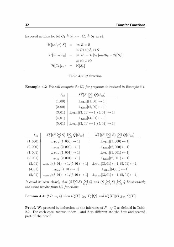
Example 4.2 We will compute the Kp? for programs introduced in Example 2.1.
`ex Kp?[[S ��
{g,p}Q]](`ex)
(1, 00) ⊥Mex[(1, 00) 7→ 1]
(2, 00) ⊥Mex[(2, 00) 7→ 1]
(3, 01) ⊥Mex[(3, 01) 7→ 1, (5, 01) 7→ 1]
(4, 01) ⊥Mex[(4, 01) 7→ 1]
(5, 01) ⊥Mex[(3, 01) 7→ 1, (5, 01) 7→ 1]
`ex Kp?[[(S ��
{}S) ��
{g,p}Q]](`ex) Kp
?[[(S ��{g,p}
S) ��{g,p}
Q]](`ex)
(1, 000) ⊥Mex[(1, 000) 7→ 1] ⊥Mex[(1, 000) 7→ 1]
(2, 000) ⊥Mex[(2, 000) 7→ 1] ⊥Mex[(2, 000) 7→ 1]
(1, 001) ⊥Mex[(1, 001) 7→ 1] ⊥Mex[(1, 001) 7→ 1]
(2, 001) ⊥Mex[(2, 001) 7→ 1] ⊥Mex[(2, 001) 7→ 1]
(3, 01) ⊥Mex[(3, 01) 7→ 1, (5, 01) 7→ 1] ⊥Mex[(3, 01) 7→ 1, (5, 01) 7→ 1]
(4, 01) ⊥Mex[(4, 01) 7→ 1] ⊥Mex[(4, 01) 7→ 1]
(5, 01) ⊥Mex[(3, 01) 7→ 1, (5, 01) 7→ 1] ⊥Mex[(3, 01) 7→ 1, (5, 01) 7→ 1]
It could be seen clearly that (S ��{}
S) ��{g,p}
Q and (S ��{g,p}
S) ��{g,p}
Q have exactlythe same results from Kp
? functions.
Lemma 4.4 If P →˜̀ Q then Ks?[[P ]] ≤T Ks
?[[Q]] and Ks?[[P ]](˜̀) ≤M Es
? [[P ]].
Proof. We proceed by induction on the inference of P →˜̀ Q as defined in Table2.2. For each case, we use index 1 and 2 to differentiate the first and secondpart of the proof.

4.3 Killed Actions 33
The case [Prefix ]:
1.
Ks?[[(α
`, r).S]] = Ks[[(α`, r).S]]envK
= >T[` 7→ ⊥M[` 7→ 1]] uT Ks[[S]]envK
≤T Ks[[S]]envK = Ks?[[S]]
as required.
2.
Ks?[[(α
`, r).S]](˜̀) = Ks[[(α`, r).S]]envK(˜̀)= >T[` 7→ ⊥M[` 7→ 1]](˜̀) uT Ks[[S]]envK(˜̀)= Es
? [[(α`, r).S]] uT Ks[[S]]envK(˜̀)≤M Es
? [[(α`, r).S]]
as required.
The case [Choice1 ]:
1. From Induction hypothesis, we knowKs
?[[S′1]] ≤T Ks
?[[S1]] which means Ks[[S1]]envK ≤T Ks[[S′1]]envK .Since S1 is part of S1 +S2, when calculating Ks[[S1]]envK , we shouldtake the effect caused by S1 + S2 into account. Here we shall have
Ks[[S1]]envS1+S2 = let [(α`11 , r1).Q1, · · · , (α`n
n , rn).Qn] = H[[S1 + S2]]
and [(α`11 , r1).Q1, · · · , (α`k
k , rk).Qk] = H[[S1]]where k <= n
in uT i∈(1,··· ,k)(>T[`i 7→ M ] uT Ks[[Qi]]env)
where M = Es[[Σi∈(1,··· ,n)(α`ii , ri).Qi]]envE
recall that
Ks[[S1 + S2]]env = let [(α`11 , r1).Q1, · · · , (α`n
n , rn).Qn] = H[[S1 + S2]]in uT i∈(1,··· ,n)(>T[`i 7→ M ] uT Ks[[Qi]]env)
where M = Es[[Σi∈(1,··· ,n)(α`ii , ri).Qi]]envE
thus, it is straightforward to see thatKs[[S1+S2]]envK ≤T Ks[[S1]]envS1+S2K ,
so we have Ks[[S1 + S2]]envK ≤T Ks[[S1]]envS1+S2K ≤T Ks[[S′1]]envK
and this proves the result.
2. from Ks[[S1 + S2]]env above, it is easy to see thatKs
?[[S1+S2]](˜̀) ≤M Es? [[S1+S2]] since clause for M equals the exposed
actions of S1 + S2.

34 Transfer Functions
The case [Choice2 ]: Analogous.
The case [ConstC ]:
1. From the induction hypothesis, we knowKs
?[[S]] ≤T Ks?[[S
′]]. We also know Ks?[[C]] = Ks
?[[S]] because Cdef= S, so
Ks?[[C]] ≤T Ks
?[[S′]] as required.
2. From the induction hypothesis, we knowKs
?[[S]](˜̀) ≤M Es? [[S]] We also know Ks
?[[C]](˜̀) = Ks?[[S]](˜̀) because
Cdef= S, so Ks
?[[C]](˜̀) ≤M Es? [[S]]
�
Lemma 4.5 If P →α(`,ı) Q then Kp[[P ]]ın ≤Tex Kp[[Q]]ın
and Kp[[P ]]ın( ˜̀ı) ≤Mex Ep[[P ]]ın .If P →α(`,ı) Q then Kp
?[[P ]] ≤Tex Kp?[[Q]] and Ks
?[[P ]]( ˜̀ı) ≤Mex Es? [[P ]].
Proof. We will prove the first part, which will immediately illustrate the cor-rectness of the second part.
We proceed by induction on the inference of P →e`ı Q as defined in Table 2.3.
The method we adopt here is exactly the same as the one used when we provethe counterpart in Lemma 4.2.
The case [Prefix,Choice1,Choice2 and ConstC ]: Refer proof ofConstS.
The case [ConstS ]:
1. This component could be regarded as the axiom of all model compo-nent rule. The induction hypothesis is P →α` P ′, from Lemma 4.4,we have Ks
?[[P ]] ≤T Ks?[[P
′]], we also have Ks?[[P ]] = Ks
?[[S]]. Thus weget Ks
?[[S]] ≤T Ks?[[P
′]].From the definition of Kp[[P ′]]ın , Kp[[S]]ın and the fact Ks
?[[S]] ≤T
Ks?[[P
′]], it is easily seen that Kp[[S]]ın ≤T Kp[[P ′]]ın , and this provesthe result.
2. The induction hypothesis is P →α` P ′, from Lemma 4.4, we haveKs
?[[P ]](`) ≤M Es? [[P ]], we also have Ks
?[[P ]] = Ks?[[S]] and Es
? [[P ]] =Es
? [[S]], so we have Ks?[[S]](`) ≤M Es
? [[S]].From the definition of Kp[[S]]ın , Ep[[S]]ın and the fact Ks
?[[S]](`) ≤M
Es? [[S]], it is easily seen that Kp[[S]]ın(`, ın) ≤Mex Ep[[S]]ın , and this
proves the result.

4.3 Killed Actions 35
The case [Coop1 ]:
1. From the induction hypothesis we haveKp[[P1]]ın0 ≤Tex Kp[[P ′
1]]ın0.
If we add uTexKp[[P2]]ın1 to its both sides, we get
Kp[[P1]]ın0 uTex Kp[[P2]]ın1 ≤Tex Kp[[P ′1]]
ın0 uTex Kp[[P2]]ın1
⇔ Kp[[P1 ��L
P2]]ın ≤Tex Kp[[P ′1��
LP2]]ın
this proves the result.2. From the induction hypothesis we haveKp[[P1]]ın0(`1, ı1) ≤Mex Ep[[P1]]ın0, we can calculate
Kp[[P1 ��L
P2]]ın = Kp[[P1]]ı0 uTex Kp[[P2]]ı1
≤Tex Kp[[P1]]ı0
So we have
Kp[[P1 ��L
P2]]ın(`1, ı1) ≤Mex Kp[[P1]]ı0(`1, ı1)
≤Mex Ep[[P1]]ın0
≤Mex Ep[[P1 ��L
P2]]ın
As required.
The case [Coop2 ]: Analogous.
The case [Coop3 ]:
1. From the induction hypothesis we haveKp[[P1]]ın0 ≤Tex Kp[[P ′
1]]ın0 and Kp[[P2]]ın1 ≤Tex Kp[[P ′
2]]ın1.
so we have
Kp[[P1]]ın0 uTex Kp[[P2]]ın1 ≤Tex Kp[[P ′1]]
ın0 uTex Kp[[P ′2]]
ın1
⇔ Kp[[P1 ��L
P2]]ın ≤Tex Kp[[P ′1��
LP ′
2]]ın
this proves the result.2. From the induction hypothesis we haveKp[[P1]]ın0(`1, ı1) ≤Mex Ep[[P1]]ın0 andKp[[P2]]ın1(`1, ı1) ≤Mex Ep[[P2]]ın1.We calculate
Kp[[P1 ��L
P2]]ın = Kp[[P1]]ın0 uTex Kp[[P2]]ın1
so we have
Kp[[P1 ��L
P2]]ın(`l, ı1)(`2, ı2) = Kp[[P1 ��L
P2]]ın(`l, ı1) +Mex
Kp[[P1 ��L
P2]]ın(`2, ı2)
≤Mex Kp[[P1]]ın0(`1, ı1) +Mex Kp[[P2]]ın1(`2, ı2)≤Mex Ep[[P1]]ın0 +Mex Ep[[P2]]ın1
= Ep[[P1 ��L
P2]]ın

36 Transfer Functions
as required.
The case [Hiding1 ]:
1. From the induction hypothesis we haveKp[[P ]]ın ≤Tex Kp[[P ′]]ın . We also know Kp[[P ′]]ın = Kp[[P ′/L]]ın andKp[[P ]]ın = Kp[[P/L]]ın . So it is straightforward to see that
Kp[[P/L]]ın ≤Tex Kp[[P ′/L]]ın .
this proves the result.
2. From the induction hypothesis we have Kp[[P ]]ın(`, ı) ≤Mex Ep[[P ]]ın
We also know Kp[[P ]]ın = Kp[[P/L]]ın and Ep[[P ]]ın = Ep[[P/L]]ın . Soit is straightforward to see that
Kp[[P/L]]ın(`, ı) ≤Mex Ep[[P/L]]ın .
The case [Hiding2 ]: Analogous.
This complete the proof of the first part. For the second part, since Kp?[[Q]] =
Kp[[Q]]ı0 , Kp?[[P ]] = Kp[[P ]]ı0 and Ep
? [[P ]] = Ep[[P ]]ı0 , when combined with the firstpart, it is straightforward to see the second part holds. �
Turning to the implementation of the least fixed point we use a simple iterativeprocedure that is terminated when Fj
K(env>T) = Fj+1
K (env>T). This procedure
works because the lattice of interest admits no infinite descending chains.
4.4 The Transfer Function
In the classic Bit Vector Frameworks the transfer function looks like the followingformula:
fblock(E) = (E \ killblock) ∪ genblock
For a forward analysis, E is the information holding at the entry of the block,killblock is the information killed by executing this block, while genblock is theinformation created by it. In our scenario, E is the extra extended multiset Mex
that tells all current available exposed actions. The block itself will be identifiedby ’ ˜̀ı’ that may be executed, where ˜̀ı ∈ Labex∪ (Labex×Labex). We comeup with our transfer function which takes the following form:
transfere`ı(E) = (E −M Kp
?[[P ]]( ˜̀ı)) +M Gp? [[P ]]( ˜̀ı)
4.4 The Transfer Function 37
We used Kp? andGp
? which are discussed in the previous section. And the transferfunction depicts how the information evolves during the execution of the modelprocesses.
From the formula we also know that the transfere`ı function is monotonic.
The following result tells that the transfer functions transfere`ı defined above
provide safe approximations to the exposed actions of the resulting process:
Proposition 4.6 If P →e`ı Q then Ep[[Q]]ın ≤Mex transfer
e`ı(Ep[[P ]]ın).
If P →e`ı Q then Ep
? [[Q]] ≤Mex transfere`ı(E
p? [[P ]]).
Proof. We will proof the first part, which will immediately illustrate the cor-rectness of the second part.
We proceed by induction on the inference of P →e`ı Q as defined in Table 2.3.
The case [Prefix ]: First observe that Gp[[(α`, r).S]]ın(`, ın) ≥Mex Ep[[S]]ın .Then
(Ep[[(α`, r).S]]ın −Mex Kp[[(α`, r).S]]ın(`, ın)) +Mex Gp[[(α`, r).S]]ın(`, ın)≥Mex Gp[[(α`, r).S]]ın(`, ın)≥Mex Ep[[S]]ın
as required.
The case [Choice1 ]: From the induction hypothesis we have
(Ep[[S1]]ın −Mex Kp[[S1]]ın(`1, ın)) +Mex Gp[[S1]]ın(`1, ın) ≥Mex Ep[[S′1]]ın
We haveKp[[S1]]ın(`1, ın) ≥Mex Kp[[S1+S2]]ın(`1, ın) and Gp[[S1]]ın(`1, ın) ≤Mex
Gp[[S1 + S2]]ın(`1, ın), we also have Ep[[S1 + S2]]ın ≥Mex Ep[[S1]]ın .
So we get
(Ep[[S1 + S2]]ın −Mex Kp[[S1 + S2]]ın(`1, ın)) +Mex Gp[[S1 + S2]]ın(`1, ın)≥Mex (Ep[[S1]]ın −Mex Kp[[S1]]ın(`1, ın)) +Mex Gp[[S1]]ın(`1, ın)≥Mex Ep[[S′1]]
ın
where we have use the monotonicity of +Mex and that −Mex is monotonicin its left argument and anti-monotonic in its right argument as stated inFact 3.5. This proves the result.

38 Transfer Functions
The case [Choice2 ]: Analogous.
The case [ConstC ]: From the induction hypothesis we have
(Ep[[S]]ın −Mex Kp[[S]]ın(`, ın)) +Mex Gp[[S]]ın(`, ın) ≥Mex Ep[[S′]]ın
Because Cdef= S, we have Ep[[S]]ın = Ep[[C]]ın ,Kp[[S]]ın = Kp[[C]]ınandGp[[S]]ın =
Gp[[C]]ın .
Thus we have
(Ep[[C]]ın −Mex Kp[[C]]ın(`, ın)) +Mex Gp[[C]]ın(`, ın) ≥Mex Ep[[S′]]ın
And this proves the result.
The case [Coop1 ]: From the induction hypothesis we have
Ep[[P ′1]]
ın ≤Mex (Ep[[P1]]ın0 −Mex Kp[[P1]]ın0(`1, ı1)) +Mex Gp[[P1]]ın0(`1, ı1)≤Mex (Ep[[P1]]ın0 −Mex Kp[[P1 ��
LP2]]ın(`1, ı1))
+MexGp[[P1 ��L
P2]]ın(`1, ı1)
using Kp[[P1]]ın0(`1, ı1) ≥Mex Kp[[P1+P2]]ın(`1, ı1), Gp[[P1]]ın0(`1, ı1) ≤Mex
Gp[[P1 + P2]]ın(`1, ı1) and the monotonicity of +Mex and that −Mex ismonotonic in its left argument and anti-monotonic in its right argumentas stated in Fact 3.5.
We can calculate
Ep[[P ′1��
LP2]]ın = Ep[[P ′
1]]ın0 +Mex Ep[[P2]]ın1
≤Mex (Ep[[P1]]ın0 −Mex Kp[[P1 ��L
P2]]ın(`1, ı1))
+MexGp[[P1 ��L
P2]]ın(`1, ı1)) +Mex Ep[[P2]]ı1
= (Ep[[P1]]ın0 +Mex Ep[[P2]]ı1)−Mex Kp[[P1 ��L
P2]]ın(`1, ı1)
+MexGp[[P1 ��L
P2]]ın(`1, ı1))
= (Ep[[P1 ��L
P2]]ın −Mex Kp[[P1 ��L
P2]]ın(`1, ı1))
+MexGp[[P1 ��L
P2]]ın(`1, ı1))
where we use Ep[[P1]]ın0 ≥Mex Kp[[P1]]ın0(`1, ı1) ≥Mex Kp[[P1+P2]]ın(`1, ı1)(Lemma 4.4) and Fact 3.6. And this proves the result.
The case [Coop2 ]: Analogous.
The case [Coop3 ]: As in the previous case, from induction hypothesis wehave
Ep[[P ′1]]
ın ≤Mex Ep[[P1]]ın0 −Mex Kp[[P1]]ın0(`1, ı1) +Mex Gp[[P1]]ın0(`1, ı1)Ep[[P ′
2]]ın ≤Mex Ep[[P2]]ın1 −Mex Kp[[P2]]ın1(`2, ı2) +Mex Gp[[P2]]ın1(`2, ı2)

4.4 The Transfer Function 39
We can calculate
Ep[[P ′1��
LP ′
2]]ın = Ep[[P ′
1]]ın0 +Mex Ep[[P ′
2]]ın1
≤Mex Ep[[P1]]ın0 −Mex Kp[[P1]]ın0(`1, ı1) +Mex Gp[[P1]]ın0(`1, ı1)+MexEp[[P2]]ın1 −Mex Kp[[P2]]ın1(`2, ı2) +Mex Gp[[P2]]ın1(`2, ı2)
= (Ep[[P1 ��L
P2]]ın −Mex Kp[[P1 ��L
P2]]ın(`1, ı1))
+MexGp[[P1 ��L
P2]]ın(`1, ı1))
using Lemma 4.4 and Fact 3.6. This proves the result.
The case [Hiding1 ]: From the induction hypothesis we have
(Ep[[P ]]ın −Mex Kp[[P ]]ın(`, ı)) +Mex Gp[[P ]]ın(`, ı) ≥Mex Ep[[P ′]]ın
Because we have Ep[[P ′/L]]ın = Ep[[P ′]]ın , Ep[[P/L]]ın = Ep[[P ]]ın ,Kp[[P/L]]ın = Kp[[P ]]ın and Gp[[P/L]]ın = Gp[[P ]]ın .
Thus we have
(Ep[[P/L]]ın −Mex Kp[[P/L]]ın(`, ı)) +Mex Gp[[P/L]]ın(`, ı) ≥Mex Ep[[P ′/L]]ın
And this proves the result.
The case [Hiding2 ]: Analogous.
The case [ConstS ]: Analogous to the case ConstS.
This complete the proof of the first part. For the second part, since Ep? [[Q]] =
Ep[[Q]]0 and Ep? [[P ]] = Ep[[P ]]0, when combined with the first part, it is straight-
forward to see the second part holds.
�

40 Transfer Functions

Chapter 5
Constructing the Automaton
Given a programlet C1 , S1; · · · ;Ck , Sk in P0
we shall now construct a finite automaton that would reflect the potentiallyinfinite transition of the system by a finite transition of the the automaton.Our automaton will have the following important components:
Q: It describes a set of states. Each state q ∈ Q is associated with an extraextended multiset E[q] that represent the current exposed actions of thatstate. In particular, q represent a certain process P with Ep
? [[P ]] ≤M E[q].
q0: q0 is the initial state of the automaton, it directly determines the exposedactions Ep
? [[P0]] of the initial process.
E: E is a map that associate each state q ∈ Q to the exposed actions of thatstate.
δ: A transition relation δ containing transitions of the following two forms:
• qs ⇒α(`1,ı1)(`2,ı2)
qt reflecting that in state qs two processes with thesame cooperation action type under the same effective cooperationscope(cf. Subsection 5.3) labeled `1 and `2 on layers ı1 and ı2, re-spectively, may interact and give rise to the state qt.
42 Constructing the Automaton
q_0
q_1(<1,000>:<3,01>)
q_2
(<1,001>:<3,01>)
q_3
<4,01>
q_4<4,01>
(<2,000>:<5,01>)
q_5
(<1,001>:<3,01>)
(<2,001>:<5,01>)(<1,000>:<3,01>) q_6
<4,01>
(<2,001>:<5,01>)
(<2,000>:<5,01>)
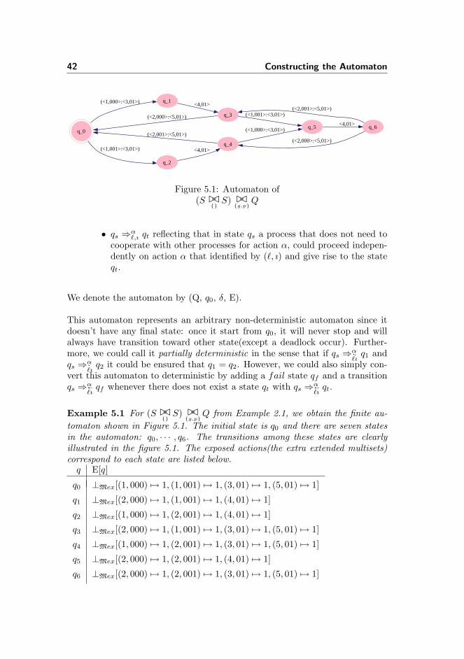
Figure 5.1: Automaton of(S ��
{}S) ��
{g,p}Q
• qs ⇒α`,ı qt reflecting that in state qs a process that does not need to
cooperate with other processes for action α, could proceed indepen-dently on action α that identified by (`, ı) and give rise to the stateqt.
We denote the automaton by (Q, q0, δ, E).
This automaton represents an arbitrary non-deterministic automaton since itdoesn’t have any final state: once it start from q0, it will never stop and willalways have transition toward other state(except a deadlock occur). Further-more, we could call it partially deterministic in the sense that if qs ⇒α
e`ıq1 and
qs ⇒αe`ı
q2 it could be ensured that q1 = q2. However, we could also simply con-vert this automaton to deterministic by adding a fail state qf and a transitionqs ⇒α
e`ıqf whenever there does not exist a state qt with qs ⇒α
e`ıqt.
Example 5.1 For (S ��{}
S) ��{g,p}
Q from Example 2.1, we obtain the finite au-tomaton shown in Figure 5.1. The initial state is q0 and there are seven statesin the automaton: q0, · · · , q6. The transitions among these states are clearlyillustrated in the figure 5.1. The exposed actions(the extra extended multisets)correspond to each state are listed below.
q E[q]
q0 ⊥Mex[(1, 000) 7→ 1, (1, 001) 7→ 1, (3, 01) 7→ 1, (5, 01) 7→ 1]
q1 ⊥Mex[(2, 000) 7→ 1, (1, 001) 7→ 1, (4, 01) 7→ 1]
q2 ⊥Mex[(1, 000) 7→ 1, (2, 001) 7→ 1, (4, 01) 7→ 1]
q3 ⊥Mex[(2, 000) 7→ 1, (1, 001) 7→ 1, (3, 01) 7→ 1, (5, 01) 7→ 1]
q4 ⊥Mex[(1, 000) 7→ 1, (2, 001) 7→ 1, (3, 01) 7→ 1, (5, 01) 7→ 1]
q5 ⊥Mex[(2, 000) 7→ 1, (2, 001) 7→ 1, (4, 01) 7→ 1]
q6 ⊥Mex[(2, 000) 7→ 1, (2, 001) 7→ 1, (3, 01) 7→ 1, (5, 01) 7→ 1]

5.1 The worklist algorithm 43
The key algorithm for constructing the automaton is a worklist algorithm andit is represented in Subsection 5.1. It starts out from the initial state q0 andconstructs the automaton by adding more and more states and transitions. Thealgorithm makes use of several auxiliary functions that will be further introducedin the subsequent subsections:
• Given a state qs representing some exposed actions we need to select thoselabels ˜̀ı (which represent actions) that may interact in the next step; this isdone using the procedure enabled described in Subsection 5.3. However,to help solving the scope problem (we will talk about it later), we alsodeveloped the auxiliary function Y?.
• Once the label-layer pair ˜̀ı has been selected we can use the functiontransfer
e`ı already introduced in the previous chapter and this could de-termine the denotation of exposed actions from this transition for thetarget state.
• Finally, a target state qt should be generated by combining information ofthe previous states and the contribution to the target state given by thecurrent transfer function.
In the last part of this chapter, we will give result of the overall correctnessof the construction.
5.1 The worklist algorithm
The main data structures of the algorithm are:
• a set Q of the states introduced so far; for each state q the table E willspecify the associated extra extended multiset E[q]∈ Mex .
• a worklist W being a subset of Q, which contains those states that haveto be processed.
• a set δ of triples (qs, ˜̀ı, qt) defining the current transitions; here qs ∈ Q isthe source state, qt ∈ Q is the target state and ˜̀ı ∈ Labex ∪ (Labex ×Labex) is the label-layer pair of edge.
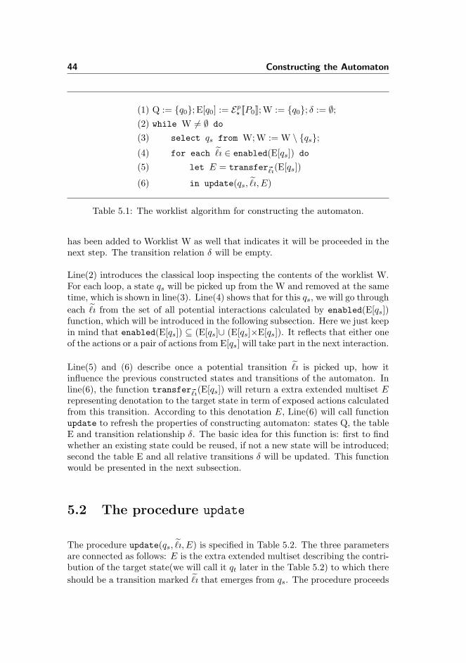
The overall algorithm has been displayed in Table 5.1 and is explained below.
Line(1) describes the initialization of the program: first the set of states Q isinitialized to contain q0 and the associated entry in table E is set to Ep
? [[P0]]. q0
44 Constructing the Automaton
(1) Q := {q0}; E[q0] := Ep? [[P0]];W := {q0}; δ := ∅;
(2) while W 6= ∅ do
(3) select qs from W;W := W \ {qs};(4) for each ˜̀ı ∈ enabled(E[qs]) do
(5) let E = transfere`ı(E[qs])
(6) in update(qs, ˜̀ı, E)
Table 5.1: The worklist algorithm for constructing the automaton.
has been added to Worklist W as well that indicates it will be proceeded in thenext step. The transition relation δ will be empty.
Line(2) introduces the classical loop inspecting the contents of the worklist W.For each loop, a state qs will be picked up from the W and removed at the sametime, which is shown in line(3). Line(4) shows that for this qs, we will go througheach ˜̀ı from the set of all potential interactions calculated by enabled(E[qs])function, which will be introduced in the following subsection. Here we just keepin mind that enabled(E[qs]) ⊆ (E[qs]∪ (E[qs]×E[qs]). It reflects that either oneof the actions or a pair of actions from E[qs] will take part in the next interaction.
Line(5) and (6) describe once a potential transition ˜̀ı is picked up, how itinfluence the previous constructed states and transitions of the automaton. Inline(6), the function transfer
e`ı(E[qs]) will return a extra extended multiset Erepresenting denotation to the target state in term of exposed actions calculatedfrom this transition. According to this denotation E, Line(6) will call functionupdate to refresh the properties of constructing automaton: states Q, the tableE and transition relationship δ. The basic idea for this function is: first to findwhether an existing state could be reused, if not a new state will be introduced;second the table E and all relative transitions δ will be updated. This functionwould be presented in the next subsection.
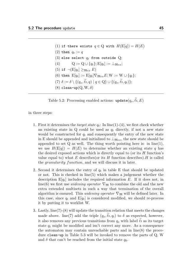
5.2 The procedure update
The procedure update(qs, ˜̀ı, E) is specified in Table 5.2. The three parametersare connected as follows: E is the extra extended multiset describing the contri-bution of the target state(we will call it qt later in the Table 5.2) to which thereshould be a transition marked ˜̀ı that emerges from qs. The procedure proceeds
5.2 The procedure update 45
(1) if there exists q ∈ Q with H(E[q]) = H(E)(2) then qt := q
(3) else select qt from outside Q;(4) Q := Q ∪ {qt}; E[qt] := ⊥Mex;(5) if ¬(E[qt] ≥Mex E)(6) then E[qt] := E[qt]∇MexE;W := W ∪ {qt};(7) δ := δ \ {(qs, ˜̀ı, q) | q ∈ Q} ∪ {(qs, ˜̀ı, qt)};(8) clean-up(Q,W, δ)
Table 5.2: Processing enabled actions: update(qs, ˜̀ı, E)
in three steps:
1. First it determines the target state qt: In line(1)-(4), we first check whetheran existing state in Q could be used as qt directly, if not a new statewould be constructed for qt and consequently the entry of the new statein E should be appended and initialized to ⊥Mex, the new state should beappended to set Q as well. The thing worth pointing here is: in line(1),we use H(E[q]) = H(E) to determine whether an existing state q hasthe desired exposed actions which is directly equal to (or its H function’svalue equal to) what E describes(or its H function describes).H is calledthe granularity function, and we will discuss it in later.
2. Second it determines the entry of qt in table E that should be updatedor not. This is checked in line(5) which makes a judgement whether thedescription E[qt] includes the required information E. If it does not, inline(6) we first use widening operator ∇M to combine the old and the newextra extended multisets in such a way that termination of the overallalgorithm is ensured. This widening operator ∇M will be defined later. Inthis case, since qt and E[qt] is considered modified, we should re-processit by putting it to worklist W.
3. Lastly, line(7)-(8) will update the transition relation that meets the changesmade above. line(7) add the triple (qs, ˜̀ı, qt) to δ as expected, however,it also removes any previous transitions from qs with label ˜̀ı as its targetstate qt might be modified and isn’t correct any more. As a consequencethe automaton may contain unreachable parts and in line(8) the proce-dure clean-up in Table 5.3 will be invoked to remove the parts of Q, Wand δ that can’t be reached from the initial state q0.
46 Constructing the Automaton
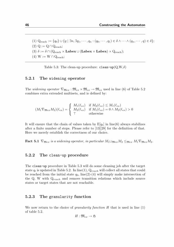
(1) Qreach := {q0} ∪ {q | ∃n,∃q1, · · · , qn : (q0, · · · , q1) ∈ δ ∧ · · · ∧ (qn, · · · , q) ∈ δ};(2) Q := Q ∩Qreach;(3) δ := δ ∩ (Qreach × Labex ∪ (Labex× Labex)×Qreach);(4) W := W ∩Qreach;
Table 5.3: The clean-up procedure: clean-up(Q,W,δ)
5.2.1 The widening operator
The widening operator ∇Mex : Mex ×Mex → Mex used in line (6) of Table 5.2combines extra extended multisets, and is defined by:
(M1∇MexM2)(`ex) =
M1(`ex) if M2(`ex) ≤ M1(`ex)M2(`ex) if M1(`ex) = 0 ∧M2(`ex) > 0> otherwise
It will ensure that the chain of values taken by E[qt] in line(6) always stabilizesafter a finite number of steps. Please refer to [13][28] for the definition of that.Here we merely establish the correctness of our choice.
Fact 5.1 ∇Mex is a widening operator, in particular M1tMexM2 ≤Mex M1∇MexM2.
5.2.2 The clean-up procedure
The clean-up procedure in Table 5.3 will do some cleaning job after the targetstate qt is updated in Table 5.2. In line(1), Qreach will collect all states that couldbe reached from the initial state q0, line(2)-(4) will simply make intersection ofthe Q, W with Qreach and remove transition relations which include sourcestates or target states that are not reachable.
5.2.3 The granularity function
We now return to the choice of granularity function H that is used in line (1)of table 5.2.
H : Mex → H

5.2 The procedure update 47
The function HL,k (for k ∈ N ∪ {>} and L ⊆ Labex) is one example of agranularity function:
HL,k(E) = {(`ex, n) | `ex ∈ L ∧ E(`ex) = n ≤ k}∪ {(`ex,>) | `ex ∈ L ∧ E(`ex) = n > k ∨ E(`ex) = >}
To ensure the correct operation of the algorithm we shall be interested in gran-ularity functions with certain properties:
• H is finitary if for all choices of finite sets Labexfin ⊆ Labex, H shouldbe
H : (Labexfin → N ∪ {>}) → Hfin
for some finite subset Hfin ⊆ H.
• H is stable if:
H(E1) = H(E2) implies H(E1∇MexE2) = H(Ei) for i = 1, 2
Fact 5.2 The granularity function HL,k is finitary as well as stable (for allchoices of L ⊆ Labex and k ≥ 0, but k 6= >).
Now we state a general termination result for the construction of the finiteautomaton:
Theorem 5.3 Whenever the algorithm of Table 5.1 terminates it produces apartially deterministic automaton.If the granularity function H is stable then the automaton satisfy the followinginjective property:
∀q1, q2 ∈ Q : H(E[q1]) = H(E[q2]) ⇒ q1 = q2
If the granularity function H is finitary then the algorithm always terminates.
Proof. The proof is similar to the counterpart exhibits in [16], we omit it here.�
Even though Fact 5.2 doesn’t guarantee that when k = >, HL,k is still finitaryas well as stable (which could ensure the algorithm of Table 5.1 terminate (Refer
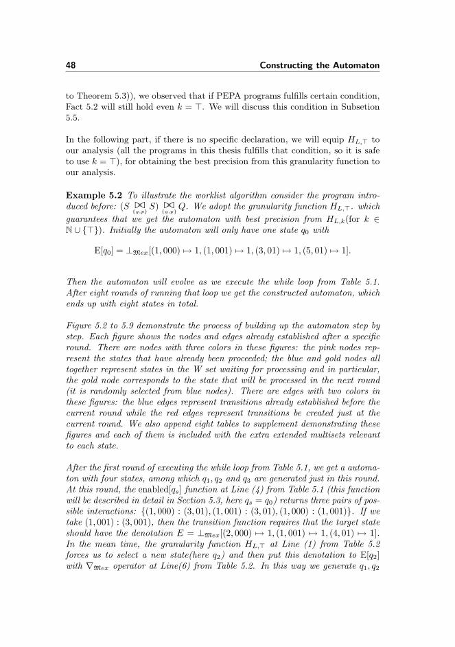
48 Constructing the Automaton
to Theorem 5.3)), we observed that if PEPA programs fulfills certain condition,Fact 5.2 will still hold even k = >. We will discuss this condition in Subsetion5.5.
In the following part, if there is no specific declaration, we will equip HL,> toour analysis (all the programs in this thesis fulfills that condition, so it is safeto use k = >), for obtaining the best precision from this granularity function toour analysis.
Example 5.2 To illustrate the worklist algorithm consider the program intro-duced before: (S ��
{g,p}S) ��
{g,p}Q. We adopt the granularity function HL,>. which
guarantees that we get the automaton with best precision from HL,k(for k ∈N ∪ {>}). Initially the automaton will only have one state q0 with
E[q0] = ⊥Mex[(1, 000) 7→ 1, (1, 001) 7→ 1, (3, 01) 7→ 1, (5, 01) 7→ 1].
Then the automaton will evolve as we execute the while loop from Table 5.1.After eight rounds of running that loop we get the constructed automaton, whichends up with eight states in total.
Figure 5.2 to 5.9 demonstrate the process of building up the automaton step bystep. Each figure shows the nodes and edges already established after a specificround. There are nodes with three colors in these figures: the pink nodes rep-resent the states that have already been proceeded; the blue and gold nodes alltogether represent states in the W set waiting for processing and in particular,the gold node corresponds to the state that will be processed in the next round(it is randomly selected from blue nodes). There are edges with two colors inthese figures: the blue edges represent transitions already established before thecurrent round while the red edges represent transitions be created just at thecurrent round. We also append eight tables to supplement demonstrating thesefigures and each of them is included with the extra extended multisets relevantto each state.
After the first round of executing the while loop from Table 5.1, we get a automa-ton with four states, among which q1, q2 and q3 are generated just in this round.At this round, the enabled[qs] function at Line (4) from Table 5.1 (this functionwill be described in detail in Section 5.3, here qs = q0) returns three pairs of pos-sible interactions: {(1, 000) : (3, 01), (1, 001) : (3, 01), (1, 000) : (1, 001)}. If wetake (1, 001) : (3, 001), then the transition function requires that the target stateshould have the denotation E = ⊥Mex[(2, 000) 7→ 1, (1, 001) 7→ 1, (4, 01) 7→ 1].In the mean time, the granularity function HL,> at Line (1) from Table 5.2forces us to select a new state(here q2) and then put this denotation to E[q2]with ∇Mex operator at Line(6) from Table 5.2. In this way we generate q1, q2
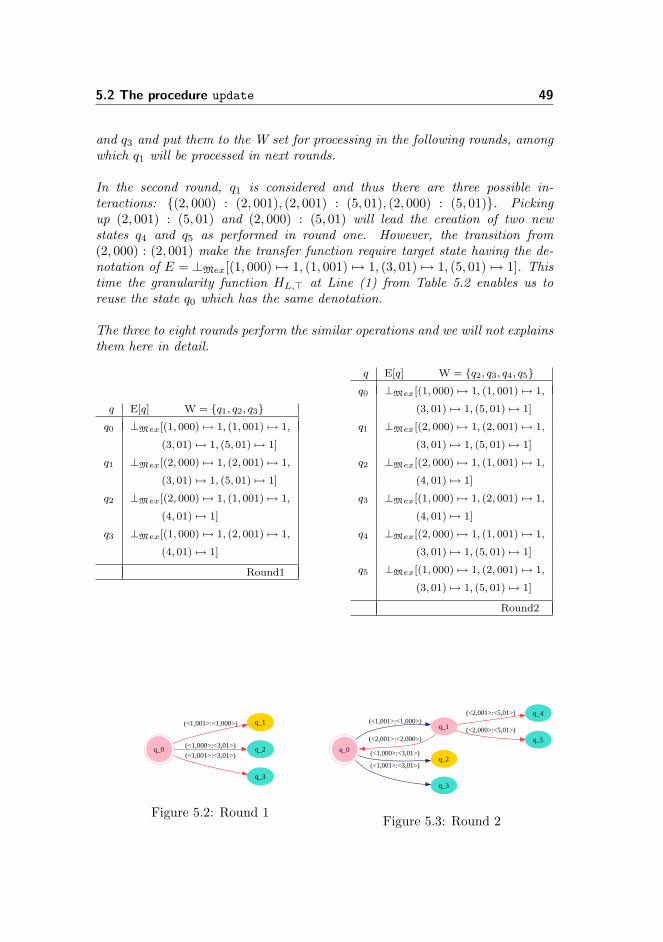
5.2 The procedure update 49
and q3 and put them to the W set for processing in the following rounds, amongwhich q1 will be processed in next rounds.
In the second round, q1 is considered and thus there are three possible in-teractions: {(2, 000) : (2, 001), (2, 001) : (5, 01), (2, 000) : (5, 01)}. Pickingup (2, 001) : (5, 01) and (2, 000) : (5, 01) will lead the creation of two newstates q4 and q5 as performed in round one. However, the transition from(2, 000) : (2, 001) make the transfer function require target state having the de-notation of E = ⊥Mex[(1, 000) 7→ 1, (1, 001) 7→ 1, (3, 01) 7→ 1, (5, 01) 7→ 1]. Thistime the granularity function HL,> at Line (1) from Table 5.2 enables us toreuse the state q0 which has the same denotation.
The three to eight rounds perform the similar operations and we will not explainsthem here in detail.
q E[q] W = {q1, q2, q3}q0 ⊥Mex[(1, 000) 7→ 1, (1, 001) 7→ 1,
(3, 01) 7→ 1, (5, 01) 7→ 1]
q1 ⊥Mex[(2, 000) 7→ 1, (2, 001) 7→ 1,
(3, 01) 7→ 1, (5, 01) 7→ 1]
q2 ⊥Mex[(2, 000) 7→ 1, (1, 001) 7→ 1,
(4, 01) 7→ 1]
q3 ⊥Mex[(1, 000) 7→ 1, (2, 001) 7→ 1,
(4, 01) 7→ 1]
Round1
q E[q] W = {q2, q3, q4, q5}q0 ⊥Mex[(1, 000) 7→ 1, (1, 001) 7→ 1,
(3, 01) 7→ 1, (5, 01) 7→ 1]
q1 ⊥Mex[(2, 000) 7→ 1, (2, 001) 7→ 1,
(3, 01) 7→ 1, (5, 01) 7→ 1]
q2 ⊥Mex[(2, 000) 7→ 1, (1, 001) 7→ 1,
(4, 01) 7→ 1]
q3 ⊥Mex[(1, 000) 7→ 1, (2, 001) 7→ 1,
(4, 01) 7→ 1]
q4 ⊥Mex[(2, 000) 7→ 1, (1, 001) 7→ 1,
(3, 01) 7→ 1, (5, 01) 7→ 1]
q5 ⊥Mex[(1, 000) 7→ 1, (2, 001) 7→ 1,
(3, 01) 7→ 1, (5, 01) 7→ 1]
Round2
q_0
q_1(<1,001>:<1,000>)
q_2(<1,000>:<3,01>)
q_3
(<1,001>:<3,01>)
Figure 5.2: Round 1
q_0
q_1(<1,001>:<1,000>)
q_2(<1,000>:<3,01>)
q_3
(<1,001>:<3,01>)
(<2,001>:<2,000>)
q_4(<2,001>:<5,01>)
q_5
(<2,000>:<5,01>)
Figure 5.3: Round 2

50 Constructing the Automaton
q E[q] W = {q3, q4, q5}q0 ⊥Mex[(1, 000) 7→ 1, (1, 001) 7→ 1,
(3, 01) 7→ 1, (5, 01) 7→ 1]
q1 ⊥Mex[(2, 000) 7→ 1, (2, 001) 7→ 1,
(3, 01) 7→ 1, (5, 01) 7→ 1]
q2 ⊥Mex[(2, 000) 7→ 1, (1, 001) 7→ 1,
(4, 01) 7→ 1]
q3 ⊥Mex[(1, 000) 7→ 1, (2, 001) 7→ 1,
(4, 01) 7→ 1]
q4 ⊥Mex[(2, 000) 7→ 1, (1, 001) 7→ 1,
(3, 01) 7→ 1, (5, 01) 7→ 1]
q5 ⊥Mex[(1, 000) 7→ 1, (2, 001) 7→ 1,
(3, 01) 7→ 1, (5, 01) 7→ 1]
Round3
q E[q] W = {q4, q5}q0 ⊥Mex[(1, 000) 7→ 1, (1, 001) 7→ 1,
(3, 01) 7→ 1, (5, 01) 7→ 1]
q1 ⊥Mex[(2, 000) 7→ 1, (2, 001) 7→ 1,
(3, 01) 7→ 1, (5, 01) 7→ 1]
q2 ⊥Mex[(2, 000) 7→ 1, (1, 001) 7→ 1,
(4, 01) 7→ 1]
q3 ⊥Mex[(1, 000) 7→ 1, (2, 001) 7→ 1,
(4, 01) 7→ 1]
q4 ⊥Mex[(2, 000) 7→ 1, (1, 001) 7→ 1,
(3, 01) 7→ 1, (5, 01) 7→ 1]
q5 ⊥Mex[(1, 000) 7→ 1, (2, 001) 7→ 1,
(3, 01) 7→ 1, (5, 01) 7→ 1]
Round4
q_0
q_1(<1,001>:<1,000>)
q_2(<1,000>:<3,01>)
q_3
(<1,001>:<3,01>)
(<2,001>:<2,000>)
q_4
(<2,001>:<5,01>)q_5(<2,000>:<5,01>)
<4,01>
Figure 5.4: Round 3
q_0 q_1(<1,001>:<1,000>)
q_2(<1,000>:<3,01>)
q_3(<1,001>:<3,01>)
(<2,001>:<2,000>)
q_4(<2,001>:<5,01>)
q_5
(<2,000>:<5,01>)
<4,01>
<4,01>
Figure 5.5: Round 4
q E[q] W = {q5, q6}q0 ⊥Mex[(1, 000) 7→ 1, (1, 001) 7→ 1,
(3, 01) 7→ 1, (5, 01) 7→ 1]
q1 ⊥Mex[(2, 000) 7→ 1, (2, 001) 7→ 1,
(3, 01) 7→ 1, (5, 01) 7→ 1]
q2 ⊥Mex[(2, 000) 7→ 1, (1, 001) 7→ 1,
(4, 01) 7→ 1]
q3 ⊥Mex[(1, 000) 7→ 1, (2, 001) 7→ 1,
(4, 01) 7→ 1]
q4 ⊥Mex[(2, 000) 7→ 1, (1, 001) 7→ 1,
(3, 01) 7→ 1, (5, 01) 7→ 1]
q5 ⊥Mex[(1, 000) 7→ 1, (2, 001) 7→ 1,
(3, 01) 7→ 1, (5, 01) 7→ 1]
q6 ⊥Mex[(2, 000) 7→ 1, (2, 001) 7→ 1,
(4, 01) 7→ 1]
Round5
q E[q] W = {q6}q0 ⊥Mex[(1, 000) 7→ 1, (1, 001) 7→ 1,
(3, 01) 7→ 1, (5, 01) 7→ 1]
q1 ⊥Mex[(2, 000) 7→ 1, (2, 001) 7→ 1,
(3, 01) 7→ 1, (5, 01) 7→ 1]
q2 ⊥Mex[(2, 000) 7→ 1, (1, 001) 7→ 1,
(4, 01) 7→ 1]
q3 ⊥Mex[(1, 000) 7→ 1, (2, 001) 7→ 1,
(4, 01) 7→ 1]
q4 ⊥Mex[(2, 000) 7→ 1, (1, 001) 7→ 1,
(3, 01) 7→ 1, (5, 01) 7→ 1]
q5 ⊥Mex[(1, 000) 7→ 1, (2, 001) 7→ 1,
(3, 01) 7→ 1, (5, 01) 7→ 1]
q6 ⊥Mex[(2, 000) 7→ 1, (2, 001) 7→ 1,
(4, 01) 7→ 1]
Round6

5.2 The procedure update 51
q_0
q_1(<1,001>:<1,000>)
q_2(<1,000>:<3,01>)
q_3
(<1,001>:<3,01>)
(<2,001>:<2,000>)
q_4
(<2,001>:<5,01>)
q_5
(<2,000>:<5,01>)
<4,01>
<4,01>
(<2,000>:<5,01>)q_6
(<1,001>:<3,01>)
Figure 5.6: Round 5
q_0 q_1(<1,001>:<1,000>)
q_2(<1,000>:<3,01>)
q_3(<1,001>:<3,01>)
(<2,001>:<2,000>)
q_4(<2,001>:<5,01>)
q_5
(<2,000>:<5,01>)
<4,01>
<4,01>
(<2,000>:<5,01>)
q_6
(<1,001>:<3,01>)
(<2,001>:<5,01>)
(<1,000>:<3,01>)
Figure 5.7: Round 6
q E[q] W = {q7}q0 ⊥Mex[(1, 000) 7→ 1, (1, 001) 7→ 1,
(3, 01) 7→ 1, (5, 01) 7→ 1]
q1 ⊥Mex[(2, 000) 7→ 1, (2, 001) 7→ 1,
(3, 01) 7→ 1, (5, 01) 7→ 1]
q2 ⊥Mex[(2, 000) 7→ 1, (1, 001) 7→ 1,
(4, 01) 7→ 1]
q3 ⊥Mex[(1, 000) 7→ 1, (2, 001) 7→ 1,
(4, 01) 7→ 1]
q4 ⊥Mex[(2, 000) 7→ 1, (1, 001) 7→ 1,
(3, 01) 7→ 1, (5, 01) 7→ 1]
q5 ⊥Mex[(1, 000) 7→ 1, (2, 001) 7→ 1,
(3, 01) 7→ 1, (5, 01) 7→ 1]
q6 ⊥Mex[(2, 000) 7→ 1, (2, 001) 7→ 1,
(4, 01) 7→ 1]
q7 ⊥Mex[(1, 000) 7→ 1, (1, 001) 7→ 1,
(4, 01) 7→ 1]
Round7
q E[q] W = {}q0 ⊥Mex[(1, 000) 7→ 1, (1, 001) 7→ 1,
(3, 01) 7→ 1, (5, 01) 7→ 1]
q1 ⊥Mex[(2, 000) 7→ 1, (2, 001) 7→ 1,
(3, 01) 7→ 1, (5, 01) 7→ 1]
q2 ⊥Mex[(2, 000) 7→ 1, (1, 001) 7→ 1,
(4, 01) 7→ 1]
q3 ⊥Mex[(1, 000) 7→ 1, (2, 001) 7→ 1,
(4, 01) 7→ 1]
q4 ⊥Mex[(2, 000) 7→ 1, (1, 001) 7→ 1,
(3, 01) 7→ 1, (5, 01) 7→ 1]
q5 ⊥Mex[(1, 000) 7→ 1, (2, 001) 7→ 1,
(3, 01) 7→ 1, (5, 01) 7→ 1]
q6 ⊥Mex[(2, 000) 7→ 1, (2, 001) 7→ 1,
(4, 01) 7→ 1]
q7 ⊥Mex[(1, 000) 7→ 1, (1, 001) 7→ 1,
(4, 01) 7→ 1]
Round8

52 Constructing the Automaton
q_0 q_1(<1,001>:<1,000>)
q_2(<1,000>:<3,01>)
q_3
(<1,001>:<3,01>)
(<2,001>:<2,000>)
q_4
(<2,001>:<5,01>)
q_5
(<2,000>:<5,01>)
<4,01>
<4,01>
(<2,000>:<5,01>)
q_6
(<1,001>:<3,01>)
(<2,001>:<5,01>)
(<1,000>:<3,01>)
<4,01> q_7(<2,001>:<2,000>)
Figure 5.8: Round 7
q_0
q_1(<1,001>:<1,000>)
q_2
(<1,000>:<3,01>)
q_3(<1,001>:<3,01>)
(<2,001>:<2,000>)
q_4
(<2,001>:<5,01>)
q_5(<2,000>:<5,01>)
<4,01>
<4,01>
(<2,000>:<5,01>)
q_6(<1,001>:<3,01>)
(<2,001>:<5,01>)(<1,000>:<3,01>)
<4,01>
q_7(<2,001>:<2,000>)
<4,01>
(<1,001>:<1,000>)
Figure 5.9: Round 8
5.3 The computation of enabled exposed actions
We now return to the construction of procedure enabled(E) used in line (4)of Table 5.1 for worklist algorithm. Here E taking the form E[qs] is an extraextended multiset that describes all potential enabled exposed actions at thatstate qs.
From Table 2.1, we know there are two kinds of transition that could take placeamong processes in PEPA.
1. The transition only involves one process. In this case, The action of thistransition should not be surrounded by any cooperation set containing thesame type. Put it more accurately, this action can’t be under any effectivecooperation scope that covers this type.
2. The transition involves two processes cooperating on the same action typewithin the same effective cooperation scope.

5.3 The computation of enabled exposed actions 53
Sequential component definition
Pdef= (α, 1).P
Qdef= (α, 2).(β, 3).Q
Model component definition
case(1): P
case(2): P ��α
Q
case(3): P ��β
Q
case(4): P ��α
(Q/{α})
Table 5.4: A example for demonstrating cooperation environment
Before introducing the concept of effective cooperation scope, we would presentcooperation environment, cooperation scope first, then we come to the termeffective cooperation scope.
Cooperation environment For the sake of determining whether an actionshould be proceeded independently or cooperate with other processes thathave the same action type, it is not enough just to analyze those processeswith the suitable action type. One also need to consider what is theircooperation environment : the cooperation dependency among differentprocesses due to the use of cooperation and hiding combinators.
Example 5.3 We define a program shown in Table 5.4: first we definetwo sequential components P and Q, then select different model componentsto illustrate the impact of various cooperation environment to action (α, 1)in process P.
In case(1), action (α, 1) is proceeded itself. In case(2), action(α, 1) inP must cooperate with action (α, 2) in Q, due to the fact they set up acooperation set{α} between themselves. However, in case(3), since thecooperation set is {β} that doesn’t cover action α, (α, 1) could still beproceeded on its own. For case(4), even though P and Q share a coopera-tion set{α},(α, 1) needn’t cooperate with (α, 2) because the hidden operatormake (α, 2) invisible to the process outside Q.
Cooperation scope Up to now, it could be seen clearly that different coopera-tion environment would make sequential components behave dissimilarly.

54 Constructing the Automaton
If take this step further, we will discuss how the cooperation and hid-den combinators impose their semantics force on the various sequentialprocesses. To make it simple, here we first present an important conceptcooperation scope to depict such semantics force: within a given program,a set of sequential processes might be influenced by a certain cooperationor hidden combinator, we say this set of sequential processes is under thecooperation scope of this certain cooperation or hidden combinator.
Recall we have defined the layer in Subsection 2.3 and this could help useasily distinguish the position of different sequential processes and theirinternal actions in a given model process. Here we borrow the conceptof layer to the cooperation and hidden combinator in order to redefinecooperation scope much more accurately. The rule for allocating layer tocooperation and hidden combinator is quite similar to the rule that appliedto actions in Subsection 2.3. The cooperation scope for either cooperationcombinators or hidden combinators is all sequential processes or actionswhose current layer is equal or lower than the combinator’s(cf. Subsection2.3, here we underline the current layer of each sequential process in thenext example).
Example 5.4 For the sequential components in Table 5.4, if we add anew model component called case(5) as follows:
case(5) : P︸︷︷︸00
��α︸︷︷︸0
( P︸︷︷︸010
��α︸︷︷︸01
( Q︸︷︷︸011
/{α}︸ ︷︷ ︸01
))
It could be easily deduced that for cooperation combinator ��α︸︷︷︸0
, processes
P︸︷︷︸00
, P︸︷︷︸010
and Q︸︷︷︸011
are under its cooperation scope. Similarly, for ��α︸︷︷︸01
,
P︸︷︷︸010
and Q︸︷︷︸011
are under its cooperation scope. For hidden combinator
/{α}︸ ︷︷ ︸01
, Q︸︷︷︸011
is under its cooperation scope.
Effective cooperation scope According to the semantics of the cooperationand hidden combinator, a cooperation combinator’s cooperation scope al-ways try to include more processes for cooperating while hidden combi-nator’s cooperation scope always intends to exclude some processes andexempt them from cooperating.
In order to merge these two kinds of cooperation scopes, we will introduceeffective cooperation scope: for any cooperation combinator with a certaintype, the effective cooperation scope should contains sequential processes

5.3 The computation of enabled exposed actions 55
under this cooperation combinator’ cooperation scope but excludes theprocesses that falls into the cooperation scope of all hidden combina-tors(whose layers are lower than the cooperation combinator of this type).Clearly if two processes are under the same effective cooperation scope ofa cooperation combinator with a certain type, they must cooperate witheach other when make a transition on that type. If a process is not underany effective cooperation scope, it could proceed independently.
Example 5.5 When scrutinizing the example 5.4 , for cooperation com-binator ��
α︸︷︷︸0
, P︸︷︷︸00
and P︸︷︷︸010
are under its effective cooperation scope; for
cooperation combinator ��α︸︷︷︸01
, its effective cooperation scope covers P︸︷︷︸010
.
And it could be seen that for process P︸︷︷︸010
, it is under both ��α︸︷︷︸0
and ��α︸︷︷︸01
’s
effective cooperation scope. This means that it must cooperate with eitherprocesses that under cooperation scope of these two cooperation combina-tors. For Q︸︷︷︸
011
, it is not under any effective cooperation scope, so the action
in it could proceed independently.
Now we will outline the significant steps in function enabled (to be presentedin Subsection 5.3.1) that calculate all potential transitions from extra extendedmultiset E.
• Given a program, for any action with type α, we need to obtain all cooper-ation and hidden combinators whose cooperation scope covers this action.This is done using the function Y describled in Subsection 5.3.2.
• Given a program, when we get the combinators(cooperation or hidden)with the right cooperation scope of all actions, we need to get the moreuseful information of their effective cooperation scope. This will leave eachaction merely to be bounded with cooperation combinators(get rid of thehidden combinators). The algorithm for doing this job is developed infunction removehidd, which will be presented in Subsection 5.3.3.
• Finally, we are able to find all enabled transitions according to the infor-mation from relevant effective cooperation scope. In particular, how tofind all actions to be cooperated among different processes is developedin function matchaction that would be further discussed in Subsection5.3.4.

56 Constructing the Automaton
5.3.1 The enabled function
The main data structure of the enabled function are:
• a map Z ∈ Y linking each action with the layer of combinators (eithercooperation or hidden) whose cooperation scope covers the action itself,where
Y = Labex → (Act× ℘(Layer)× ℘(Layer))
The first ℘(Layer) describes the set of cooperation combinators that couldbe on several layers, while the second ℘(Layer) records the similar infor-mation for hidden combinators.
• a set S ∈ U, this set contains action information and the respective coop-eration combinators whose effective cooperation scope cover this action.
U = ℘(Labex × Act × ℘(Layer))= ℘(Lab × Layer × Act × ℘(Layer))
The ℘(Layer) describes the set of cooperation combinators whose effectivecooperation scope covers this action.
• a variable R ∈ R collecting the enabled transitions from both type, where
R = ℘(Labex)× ℘(Labex× Labex)
℘(Labex) is the result for transitions involving single action while ℘(Labex×Labex) tracks all transitions involving two actions with the same type.
• E ∈ Mex taking the form E[qs] is an extra extended multiset that describesall potential enabled exposed actions at that state qs.
The overall algorithm for enabled function is displayed in Table 5.5 and is ex-plained below. The initialization are performed in line(1) and (2): First Z iscalculated by Yp
? [[P0]](0, ∅, ∅) and this function is discussed in the following Sub-section 5.3.2, here we just give its parameters’ meaning: P represents the modelcomponent of this program; 0, ∅, and ∅ respectively indicate the function willstart from the 0 layer(top layer), cooperation and hidden set for combinators isset ∅ (combinators here should has the right cooperation scope over different ac-tions) and later the function will traverse the program tree and collect necessaryinformation marked with correct layer to the cooperation and hidden set on thefly. The result of the enabled function R is initialized to ∅. Taking E and Zas parameters, line(2) obtain the value of S by removehidd function. And this
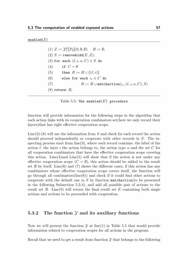
5.3 The computation of enabled exposed actions 57
enabled(E)
(1) Z := Yp? [[P0]](0, ∅, ∅); R := ∅;
(2) S := removehidd(E,Z);(3) for each (`, ı, α, C) ∈ S do
(4) if C = ∅(5) then R := R ∪ {(`, ı)}(6) else for each ıc ∈ C do
(7) R := R ∪ matchaction(ıc, (`, ı, α, C), S)(8) return R;
Table 5.5: The enabled(E) procedure
function will provide information for the following steps in the algorithm thateach action links with its cooperation combinators set(here we only record theirlayers)that has right effective cooperation scope.
Line(3)-(8) will use the information from S and check for each record the actionshould proceed independently or cooperate with other records in S. The in-specting process start from line(3), where each record contains: the label of theaction `, the layer ı the action belongs to, the action type α and the set C forall cooperation combinators that have the effective cooperation scope coveringthis action. Line(4)and Line(5) will show that if the action is not under anyeffective cooperation scope (C = ∅), this action should be added to the resultset R by itself. Line(6) and (7) shows the different cases, if this action has anycombinators whose effective cooperation scope covers itself, the function willgo through all combinators(line(6)) and check if it could find other actions tocooperate with the default one in S by function matchaction(to be presentedin the following Subsection 5.3.4), and add all possible pair of actions to theresult set R. Line(8) will return the final result set E containing both singleactions and actions to be proceeded with cooperation.
5.3.2 The function Y and its auxiliary functions
Now we will present the function Y at line(1) in Table 5.5 that would provideinformation related to cooperation scopes for all actions in the program.
Recall that we need to get a result from function Y that belongs to the following

58 Constructing the Automaton
domain:Y = Labex → (Act× ℘(Layer)× ℘(Layer))
where the first and second ℘(Layer) represent the set of combinators’ layersfor cooperation and hidden respectively. The entry in this map Labex requireseach label must link to some layer information. In other words, Label mustlinks to Layer, ℘(Layer) and ℘(Layer). The first problem is how to put eachlabel together correspond with layer information.
From the previous chapter, we already know that because of cooperation envi-ronment, an action in a certain sequential process may behave dissimilarly if itis located at different layers. Here we can conclude that the sequential processitself may also act distinctively when located at different layers. And the layerinformation of each sequential process (differentiated by sequential process nameCk) will be assigned according to the structure of the model component defini-tion.
Thus we come to the point of how to solve the problem above, which shouldhave two steps:let C1 , S1; · · · ;Ck , Sk in P0
1. For every sequential process name Ck, collect all possible labels(actions)that belong to that process (all possible actions a sequential process mightbehave as).
2. Put layer information to each sequential process name Ck which is deter-mined by the structure of the model component definition. Subsequentlyput layer information to all possible labels(actions) of different sequentialprocesses separately.
For step1 we have developed a function Ys, while at step2 a function Yp wasproposed.
The function Ys? tries to collect all action label-type pairs related for each se-
quential process name and has the functionality
Ys? : Sproc → ℘(Lab×Act)
The function is defined in Table 5.6 using the overall pattern developed in pre-vious sections. So we have a function
Ys : Sproc → (PN → ℘(Lab×Act)) → ℘(Lab×Act)

5.3 The computation of enabled exposed actions 59
Exposed actions for let C1 , S1; · · · ;Ck , Sk in P0
Ys[[(α`, r).S]]env = (`, α) ∪ Ys[[S]]env
Ys[[S1 + S2]]env = Ys[[S1]]env ∪ Ys[[S2]]env
Ys[[C]]env = env(C)Ys
? [[S]] = Ys[[S]]envY
whereFY = [C1 7→ Ys[[S1]]env, · · · , Ck 7→ Ys[[Sk]]env]and env∅ = [C1 7→ ∅, · · · , Ck 7→ ∅]and envY = tj≥0Fj
Y(env∅)
Yp[[P1 ��L
P2]](ı, coop, hidd) = let coop′ = addlayers(coop, L, ı)
in Yp[[P1]](ı0, coop′, hidd) ∪ Yp[[P2]](ı1, coop′, hidd)Yp[[P/L]](ı, coop, hidd) = let hidd′ = addlayers(hidd, L, i′)
and ı = ı′0 or ı = ı′1in Yp[[P ]](ı, coop, hidd′)
Yp[[S]](ı, coop, hidd) = let [(`1, α1), · · · , (`n, αn)] = Ys? [[S]]
in [(`1, ı) 7→ (α1, ∂(coop, α1), ∂(hidd, α1)), · · · ,
(`n, ı) 7→ (αn, ∂(coop, αn), ∂(hidd, αn))]Yp
? [[P ]](0, ∅, ∅) = Yp[[P ]](0, ∅, ∅)
Table 5.6: Ys and Yp function
whose second argument is an environment providing similar information for theprocess names. The domain ℘(Lab ×Act) inherits a partial ordering v fromthe subset ordering on sets and becomes a complete lattice. The function FYis a monotonic function on a complete lattice and hence has a least fixed pointenvY . As the function FY is in fact also continuous the Kleene formulationof the fixed point is permissible. It follows that the overall definition of Ys
? iswell-defined.
Now we turn to define the function Yp
Yp : Pproc → Y (= Pproc → (Labex → (Act× ℘(Layer)× ℘(Layer))))
It could be seen clearly that this function will return the affiliation of eachaction(to be distinguished by label and action type) and its layer information.
For function Yp, it will always take layer ı, cooperation combinator set coop andhidden combinator set hidd as parameters and finally append the correct layerinformation to each S sequential component(Finally to each actions within a S
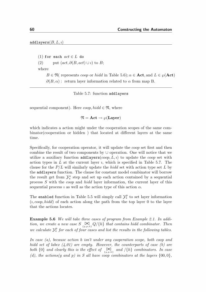
60 Constructing the Automaton
addlayers(B,L, ı)
(1) for each act ∈ L do
(2) put (act, ∂(B, act) ∪ ı) to B;where
B ∈ N( represents coop or hidd in Table 5.6); α ∈ Act, and L ∈ ℘(Act)∂(B,α) : return layer information related to α from map B.
Table 5.7: function addlayers
sequential component). Here coop, hidd ∈ N, where
N = Act → ℘(Layer)
which indicates a action might under the cooperation scopes of the same com-binator(cooperation or hidden ) that located at different layers at the sametime.
Specifically, for cooperation operator, it will update the coop set first and thencombine the result of two components by ∪ operation. One will notice that weutilize a auxiliary function addlayers(coop, L, ı) to update the coop set withaction types in L at the current layer ı, which is specified in Table 5.7. Theclause for the P/L will similarly update the hidd set with action type set L bythe addlayers function. The clause for constant model combinator will borrowthe result get from Ys
? step and set up each action contained by a sequentialprocess S with the coop and hidd layer information, the current layer of thissequential process ı as well as the action type of this action α.
The enabled function in Table 5.5 will simply call Yp? to set layer information
(ı, coop, hidd) of each action along the path from the top layer 0 to the layerthat the actions locates.
Example 5.6 We will take three cases of program from Example 2.1. In addi-tion, we create a new case S ��
{g,p,h}Q/{h} that contains hidd combinator. Then
we calculate Yp? for each of four cases and list the results in the following tables.
In case (a), because action h isn’t under any cooperation scope, both coop andhidd set of labex (4,01) are empty. However, the counterparts of case (b) areboth {0} and clearly this is the effect of ��
{g,p,h}and /{h} combinators. In case
(d), the actions(g and p) in S all have coop combinators at the layers {00, 0},

5.3 The computation of enabled exposed actions 61
due to the fact they are under the cooperation scopes of both ��{g,p}︸ ︷︷ ︸
0
and ��{g,p}︸ ︷︷ ︸00
.
Yp? of S︸︷︷︸
00
��{g,p}︸ ︷︷ ︸
0
Q︸︷︷︸01
S︸︷︷︸00
��{g,p,h}︸ ︷︷ ︸
0
( Q︸︷︷︸01
/{h}︸ ︷︷ ︸0
)
labex action coop hidd action coop hidd(1, 00) g {0} ∅ g {0} ∅(2, 00) p {0} ∅ p {0} ∅(3, 01) g {0} ∅ g {0} ∅(4, 01) h ∅ ∅ h {0} {0}(5, 01) p {0} ∅ p {0} ∅Case (a) (b)
Yp? of ( S︸︷︷︸
000
��{}︸︷︷︸00
S︸︷︷︸001
) ��{g,p}︸ ︷︷ ︸
0
Q︸︷︷︸01
( S︸︷︷︸000
��{g,p}︸ ︷︷ ︸00
S︸︷︷︸001
) ��{g,p}︸ ︷︷ ︸
0
Q︸︷︷︸01
labex action coop hidd action coop hidd(1, 000) g {0} ∅ g {00, 0} ∅(2, 000) p {0} ∅ p {00, 0} ∅(1, 001) g {0} ∅ g {00, 0} ∅(2, 001) p {0} ∅ p {00, 0} ∅(3, 01) g {0} ∅ g {0} ∅(4, 01) h ∅ ∅ h ∅ ∅(5, 01) p {0} ∅ p {0} ∅Case (c) (d)
5.3.3 The procedure removehidd
In the last subsection, we have discussed how to put the information of coop-eration scope to each actions in the program. Now we should talk about themethod to merge the information from cooperation scopes and calculate theeffective cooperation scope for each cooperation combinator to each action. Putit in another words, we will simplify each entry in map Z (cf. Table 5.5 line(2))by function removehidd that essentially utilizes layers in hidd to restrict layersin coop, and finally we will get rid of the existing hidd and coop and insteadto replace them with a new coop (cooperation combinators set) which has thetruly effective cooperation scope to this action.
Our removehidd procedure is displayed in Table 5.8. Line(1) is the initializa-tion of the procedure: S is the result set, where each element represents the

62 Constructing the Automaton
The procedure removehidd(E,Z)
(1) S := ∅;(2) for each (`, ı) ∈ domEx(E) do
(3) let (α, C, H) = Z((`, ı))(4) in if ¬(C = ∅)(5) then for each ıc ∈ C do
(6) if there exists ih ∈ H
(7) with ℵ(ıc) <= ℵ(ıh)(8) then C := C \ ıc;(9) S := S ∪ (`, ı, α, C);(10) return S;
Table 5.8: function removehidd
information of one action which has four fields: label `, layer ı, action type αand cooperation combinators set C(represent by several layers) from which allcombinators have effective cooperation scope over this action. Line(2) start theloop which checks all elements in domEx(E)(cf. Section 3.1.2 ), meaning that weonly consider exposed actions that is described in the extra extended multisetE. Line(3) get layer information of each actions to be checked.
Line(4)-(8) describes that some cooperation combinators will be blocked bysome hidden combinators for the same action. Line(4) and (5) say we will checkeach layer in C and find out if any layer should be removed from the set. Inanother words, we should determine if some cooperation combinators will losetheir cooperation scope over a certain action when taking the influence causedby some hidden combinators into account. Line(6)-(8) state that under whatspecific circumstance a layer should be removed from C: in hidd set check if thereexists any layer that is higher than the layer from the cooperation combinatorlayer set C. If the condition is guaranteed, this hidden combinator will hidethis cooperation combinator and make the action not cooperate with processesoutside the cooperation scope of this hidden combinator even though they areunder the cooperation scope of this cooperation combinator. Here function ℵ(ı)will return the length of the layer ı: the larger the value is, the lower the layeris.
Line(9) will add a new element which contains the updated C to set S. Andfinally the result will be returned by line(10).
Example 5.7 Here we will inspect four cases from Example 5.6. First we cal-

5.3 The computation of enabled exposed actions 63
culate removehidd(Ep? [[P0]],Yp
? [[P0]]) for each of them, based on the result fromExample 5.6 and Example 3.1(The result of Case(a) and (b) in Example 3.1 areexactly the same).The table below shows the result.
removehidd(Ep? [[P0]],Yp
? [[P0]])
Case(a) Case(b)labex action coop′ labex action coop′
(1, 00) g {0} (1, 00) g {0}(3, 01) g {0} (3, 01) g {0}(5, 01) p {0} (5, 01) p {0}
Case(c) Case(d)labex action coop′ labex action coop′
(1, 000) g {0} (1, 000) g {00, 0}(1, 001) g {0} (1, 001) g {00, 0}(3, 01) g {0} (3, 01) g {0}(5, 01) p {0} (5, 01) p {0}
We find that the coop′ is exactly the same as the coop in Example 5.6. Thisis because the actions considered in these cases (p,g) are not related to anyhidden combinators. Next we show a example that coop in 5.6 is modified by theremovehidd function.
Imagine the case(b) of the program is in some state qx that has extra extendmultiset E = ⊥Mex[(2, 00) 7→ 1, (4, 01) 7→ 1], then the result of removehidd(E,Yp
? [[P0]]) is
labex action coop′
(2, 00) p {0}(4, 01) h ∅
Notice that this time the coop′ of action (4, 01) is ∅ instead of the coop = {0}in Example 5.6. And clearly action (4, 01) will not cooperate with other actionssince it is hidden by /{h} combinator.
5.3.4 The procedure matchaction
The procedure matchaction(ıc, (`, ı, α, C), S) tries to find a record in S, that willcooperate with action(the default record) (`, ı, α, C) on the cooperation combi-nator on layer ıc. In Table 5.9 the function is displayed and we will explain it

64 Constructing the Automaton
matchaction(ıc, (`, ı, α, C), S)
(1) T := ∅;(2) for each (`′, ı′, α′, C ′) ∈ S do
(3) if there exists ı′c ∈ C ′ with
(4) ıc = ı′c ∧ α = α′ ∧ ¬(ρ(ı,ℵ(ıc)) = ρ(ı′,ℵ(ıc)))(5) then T := T ∪ {((`, ı), (`′, ı′))};(6) return T ;
Table 5.9: function matchaction
below. Line(1) initialize the variable T for collecting all possible exposed actionpairs under the effective cooperation scope of a certain cooperation combinatorat layer ıc.
Line(2)-(5) illustrate the matching procedure: line(2) start the loop that indi-cates we need to exam all record in S; line(3) and (4) states the condition onwhich two actions should cooperate with each other: if there is a record in Swhose cooperation combinator layer set C ′ contains a layer ı′c that meet:
• Two actions are under the same effective cooperation scope: ı′c = ıc.
• Its action type α′ is the same as the default record’s action type α.
• Two actions shouldn’t under the same side of cooperation combinator, thisis ensured by ¬(ρ(ı,ℵ(ıc)) = ρ(ı′,ℵ(ıc))). The function ρ(ı, k) return thevalue of the element at position k + 1 of layer ı. e.g. If ı = 001011, thenρ(ı, 3) will return 0.
Line(5) and(6) will append a qualified enabled action pair to the result set whenthe program goes through all the reords in S, and finally return the result. Onething worth mentioning here is that: when we try to add a new enabled actionpair to the final result set T , we assume that {(`, ı), (`′, ı′)} is the same as{(`′, ı′), (`, ı)}, which means we will only add one of them to the result set T ,not both of them.
Example 5.8 Now we are ready to compute of enable(E) function from Table5.5. Here we inspect four cases from Example 5.6, where E = Ep
? [[P0]]. Thecalculation is based on the result of Example 3.1 and Example 5.7, by utilizingthe function matchaction. The results are shown below:

5.4 Correctness result 65
enable(Ep? [[P0]])
Case (a) (b) (c) (d)(3, 01) : (1, 00) (3, 01) : (1, 00) (3, 01) : (1, 000) (3, 01) : (1, 000)
(3, 01) : (1, 001) (3, 01) : (1, 001)(1, 000) : (1, 001)
Fact 5.4 The function enabled is monotonic.
5.4 Correctness result
We now show the correctness of the automaton constructed by Table 5.1. Weshall define P B E by
P B E iff Ep? [[P ]] ≤Mex E
and say that a state denoting the extra extended multiset E represents a processP whenever P B E.
We now establish the main result which is independent of the choice of thegranularity function H:
Theorem 5.5 First suppose that the algorithm of Table 5.1 terminates andproduces a finite automaton (Q, q0, δ, E). Second suppose that If P →
e`ı Q then˜̀ı ∈ enabled(Ep? [[P ]]). Then if
P B E[qs] and P →e`ı Q
then there exists a unique qt ∈ Q such that
Q B E[qt] and (qs, ˜̀ı, qt) ∈ δ
Proof. Let us first inspect one specific transition occurred when generate theautomaton. This is related to line (4-6) of Table 5.1.
We have assumed P B E[qs], which indicates Ep? [[P ]] ≤Mex E[qs].
Since P →e`ı Q it follows that ˜̀ı ∈ enabled(E[qs]) using the second assumption
and Fact 5.4 and hence that ˜̀ı is selected for consideration in line(4) of Table5.1. It follows that line (5) of Table 5.1 produces an extra extended multiset Ethat E = transfer
e`ı(E[qs]).

66 Constructing the Automaton
By line (6) of Table 5.1 and definition of update in Table 5.2, it is immediatethat we identify a state qt in lines(1-4) of Table 5.2 and after the excution oflines (5-8) of Table 5.2 we have
(qs, ˜̀ı, qt) ∈ δ and E ≤Mex E[qt] (5.1)
Since Ep? [[P ]] ≤Mex E[qs] and the monotonicity of transfer
e`ı function, we have
transfere`ı(E
p? [[P ]]) ≤Mex transfer
e`ı(E[qs]) = E (5.2)
Since P →e`ı Q from the Proposition 4.6, we have
Ep? [[Q]] ≤Mex transfer
e`ı(Ep? [[P ]]) (5.3)
Combine equation (5.1)(5.2) and (5.3), we have
Ep? [[Q]] ≤Mex E[qt] and (qs, ˜̀ı, qt) ∈ δ
this equal to the conclusion of the theorem that
Q B E[qt] and (qs, ˜̀ı, qt) ∈ δ
The proof above try to inspect line (4-6) of Table 5.1 and capture one specifictransition P →
e`ı Q that satisfies the theorem. This could ensure (qs, ˜̀ı, qt) is inthe growing automaton after one specific transition.
However, if we consider all transitions happen during the constructing of au-tomaton, from line (5-8) of Table 5.2, we know a previously calculated qt(q inTable 5.2, which is generated by the previous transition , here we label it withqt1 ) might be removed and replaced with an new qt(see line (7) of Table 5.2,we label it with qt2). In this case,(qs, ˜̀ı, qt1) will be replaced with (qs, ˜̀ı, qt2).This doesn’t contradict our conclusion: we already have
Q B E[qt1] and (qs, ˜̀ı, qt1) ∈ δ
Because E[.] grows in a non-decreasing manner during the generation of theautomaton (that could be seen from line (6) of Table 5.2), E[qt1] ≤Mex E[qt2],from this we know Q B E[qt2]. We get
Q B E[qt2] and (qs, ˜̀ı, qt2) ∈ δ
This means even all transitions are considered, the conclusion is still correct.

5.5 Termination of the worklist Algorithm 67
The uniqueness of qt is due to the fact that automation is partially deterministic.�
The first assumption has already been established which is shown in Theory5.3. However, due to the restricted time schedule of the project, the secondassumption: suppose that If P →
e`ı Q then ˜̀ı ∈ enabled(Ep? [[P ]]), has not been
formally proved yet. Here we only give what we have already established andwhat need further investigation in order to complete the proof:
In Table 5.5, in the end we need to show: ˜̀ı ∈ R (**). Since ˜̀ı is formed fromthe set S that is at line(3) in Table 5.5, then first we need to prove:
for some α and C, (`, ı, α, C) ∈ S always holds. (*)
Since S is computed at line (2) in table 5.5, by invoking the function removehidd,we shall look into removehidd in Table 5.8. At line (3) of Table removehidd,the C and α could be easily obtained from Z((`, ı)) for each (`, ı). Here α isdirectly chosen to be part of the element of S. For C, at line(4) in Table 5.8,no matter C = ∅ is true or not, there will be a subset of C being chosen forforming an element of S. Thus, (*) holds.Then line (4)-(5)in Table 5.5) shows if C = ∅ , ˜̀ı ∈ R holds immediately, whichis the first case for proving (**). For the second case, we need to prove: ifc 6= ∅, ˜̀ı ∈ R. However, this part of proof we have not figured out yet, we guesswe should use some invariant comes from Yp
? [[P ]], and then go through functionmatchaction for completing the proof.
5.5 Termination of the worklist Algorithm
In SubSection 5.2.3, from Fact 5.2 we pinpoint that k 6= > doesn’t guarantee thegranularity function to be finitary as well as stable(finitary is the requirementfor worklist algorithm to terminate, which is stated in Theorem 5.3). We alsostate that we still adopt the granularity function with k = > for our analysis inthis thesis. Here we give the reason by discussing under what condition mustwe use the granularity function with k 6= > to ensure the algorithm terminatewhile under what condition k = > would also ensure the program terminate.
Let’s see two PEPA programs in Table 5.10 (we already annotated them withlabels and layers). They describe the same system behaviors which are writtenin two styles.

68 Constructing the Automaton
let P1 , (f1, r).P2 + P3
P2 , (g2, r).P1 + P3
P3 , (h3, r).P1
in P 01
(a)
let P1 , (f1, r).P2 + (h2, r).P1
P2 , (g3, r).P1 + (h4, r).P1
in P 01
(b)
Table 5.10: PEPA programs written in two styles
`ex Ep? [[P1]] Gp
? [[P1]](`ex) Kp?[[P1]](`ex)
(1, 0) 1 ⊥Mex[(2, 0) 7→ 1, (3, 0) 7→ 1] ⊥Mex[(1, 0) 7→ 1, (3, 0) 7→ 1]
(2, 0) 0 ⊥Mex[(1, 0) 7→ 1, (3, 0) 7→ 1] ⊥Mex[(2, 0) 7→ 1, (3, 0) 7→ 1]
(3, 0) 1 ⊥Mex[(1, 0) 7→ 1, (3, 0) 7→ 1] ⊥Mex[(3, 0) 7→ 1]
Table 5.11: functions defined for (a) in Table 5.10
The difference of these program is the behavior of P3 in program (a) is directlyadded to P1 and P2 in program (b). And consequently the program (a) will notterminate while the program (b) will. This could be explained by their kill andgen functions, which are shown in Table 5.11 and Table 5.12 respectively.
First let’s see the reason that (a) will not terminate with k = >: Initiallyaction (3,0) is enabled (from function Ep
? [[P1]]). If we take this transition, itwill kill (3,0) (from function Kp
?[[P1]]) and at the same time generate both (1,0)and (3,0) as enable actions (from function Gp
? [[P1]]). Now the system will beat state ⊥Mex[(1, 0) 7→ 2, (3, 0) 7→ 1] and we could take transition (3,0) again!Noticed the occurrence of enable action (1,0) from 1 becomes to 2, while theoccurrence of enable action (3,0) remains the same: take transition (3,0), the
`ex Ep? [[P1]] Gp
? [[P1]](`ex) Kp?[[P1]](`ex)
(1, 0) 1 ⊥Mex[(3, 0) 7→ 1, (4, 0) 7→ 1] ⊥Mex[(1, 0) 7→ 1, (2, 0) 7→ 1]
(2, 0) 1 ⊥Mex[(1, 0) 7→ 1, (2, 0) 7→ 1] ⊥Mex[(1, 0) 7→ 1, (2, 0) 7→ 1]
(3, 0) 0 ⊥Mex[(1, 0) 7→ 1, (2, 0) 7→ 1] ⊥Mex[(3, 0) 7→ 1, (4, 0) 7→ 1]
(4, 0) 0 ⊥Mex[(1, 0) 7→ 1, (2, 0) 7→ 1] ⊥Mex[(3, 0) 7→ 1, (4, 0) 7→ 1]
Table 5.12: functions defined for (b) in Table 5.10

5.5 Termination of the worklist Algorithm 69
enabled actions being generated always include the actions being killed! If wekeep executing action (3,0), the new state will contain a growing number ofenabled action (1,0) but always keeps one occurrence of action (3,0). Since inthis way all new states generated will be discriminated by granularity functionwith k = > and they can’t be reused among each other, the program will neverstop. Now it is easy to know why Fact 5.2 doesn’t hold for k = >: it is notfinitary any more: recall in Subsection 5.2.3, the definition of finitary requires tohave finite sets Labexfin. Our growing new state doesn’t satisfy this condition.
The program (b) will not suffer the problem program (a) encounters. This isbecause the kill function of (b) is much more accurate than that in program (a).Let’s see (2,0) and (4,0), they will kill themselves as well as the actions in otherbranches of the sequential process: (2,0) will kill (1,0) and (2,0); (4,0) will kill(3,0) and (4,0). However, the action (3,0) in program (a) will only kill itself,even though they stay in both P1 and P2 and should kill the branch next to it,like the action (2,0) and (4,0) in program (b) perform (from the semantic pointof view). In program (a), just executing (3,0), we don’t know weather it comesfrom P1 or P2, thus we only kill itself: it is safe to kill less!
From this example, we can see that program (b) owns the kill and gen functionsthat directly correspond to the semantics of the program, while program (a)doesn’t.
We can conjecture that if we write PEPA program in the style of program (b):always put constant sequential component into a prefix sequential component,our kill and gen function will always be accurate and they could capture thesystem behavior exactly. Since there will be no approximation any more, thesystem will only have a finite number of states.
Our PEPA programs in the thesis are all written in the style of program (b), soit is very safe to use k = > when specifying the granularity function.

70 Constructing the Automaton

Chapter 6
Accelerate the Analysis
In the previous chapters, we have defined essential domains and several auxiliaryfunctions. With worklist algorithm we build the automaton that could capturethe properties of the interactions among several sequential processes.
Each sequential process is simulated and allocated a layer depending on itsposition, determined by the model component definition of the program. So wecould actually discriminate the same actions which belong to different sequentialprocesses even though they behave exactly the same. For instance, recall twosequential processes S in Example 2.4. Their layers are determined by the modelcomponent definition as shown below:
( S︸︷︷︸000
��{}
S︸︷︷︸001
) ��{g,p}
Q︸︷︷︸01
The actions in S000 and S001 take different seats in the extra extended multisetwhen we come to the analysis. Taking the definition of S from Example 2.3,already equipped with label, we annotate the actions of S000 as: (1,000) and(2,000) while actions of S001 as: (1,001) and (2,001). The entry of extra ex-tended domain for this program will contain these four items. Since the worklistalgorithm will work on this domain, we will build an automaton that consistsof states and transitions contributed by these four items(cf. Figure 5.1).
However, sometimes we are not that concern about the difference of same actions

72 Accelerate the Analysis
between S000 and S001(for example, action labeled 1 will only be noted as (1,00)instead of (1,000), (1,001)). In this way, we could cut down the total numberof items in the domain of the analysis. In other words, we are willing to reducethe precision of the analysis by ignoring the difference of sequential processwith similar behavior. The motivation for doing so is the benefits from twoperspective:
• Generally, lowing the precision (ignore unnecessary details) is always ac-companied the speed improvement of analysis. In other words, it will cutdown the computing demands.
• In our case, we will build up a more succinct automaton that containsfewer states and transitions. Consequently the graphic representations ofthe automaton will be illustrated in fewer nodes and edges that enhancethe readability of the pictures.
In the following subsections, we will develop techniques to address this issue.
6.1 Method 1
The first method is to address the situation mentioned above: given a program,if there exists some sequential processes conjointly cooperating with each otheron ∅ set: (((S ��
{}S) ��
{}S) · · · ��
{}S) , we could group them and remain only
one sequential process S to represent all of them. Take it one step further,we could group any subparts of program together if they behave exactly thesame and conjointly cooperate on ∅. The subpart of the program could be somesequential processes operating on the hidden or cooperate combinator with nonempty set or empty set. For instance: ((S ��
{β}S)/{α}) ��
{}((S ��
{β}S)/{α}) could
be simplify to ((S ��{β}
S)/{α}).
Specifically, we will modify the analysis we have already developed in two stepsto accomplish the above goal:
Step1 First we should simplify the model component definition of the programas much as we can as long as we conform to the idea presented above.Furthermore, we will track the number of subparts(should be same) thatparticipate in grouping event. They will be used in the second step.

6.1 Method 1 73
Exposed actions for let C1 , S1; · · · ;Ck , Sk in P0
Ep[[P1 ��L
P2]]ıλ = λ·Mex(Ep[[P1]]ı0 +Mex Ep[[P2]]ı1)Ep[[P/L]]ıλ = λ·Mex(Ep[[P ]]ı)Ep[[S]]ıλ = let (`1 7→ n1, · · · , `n 7→ nn) = Es
? [[S]]in λ·Mex(⊥Mex[(`j , ı) 7→ nj ]) where `j ∈ domExlayer(⊥Mex, ı)and j ∈ {1, · · · , n}
Ep? [[P ]] = Ep[[P ]]0
Table 6.1: The redefined Ep function
Example 6.1 For instance,
(((S ��{}
S) ��{}
S)/{α}) ��{}
(((S ��{}
S) ��{}
S)/{α})
could be transformed into(S3/{α})2
where 3 is annotated to S to indicate we have three copy of S cooperating∅ , and 2 is annotated to the hidden combinators to memorize there aretwo entities of (S3/{α}).
Step2 Second we will calculate the Es? and Ep
? . Es? is defined exactly the same
as in Table 3.1. However, Ep? is redefined to take into account the number
of the same subparts of the program, which is shown in Table 6.1.
In Table 6.1, ·Mex is scalar multiplication defined by 0·MexM = ⊥Mex and(λ + 1)·MexM = (λ·MexM) +Mex M . Notice we have added a new para-meter λ to each model component Ep[[]]ıλ, representing the number of samecopy of this model component(subpart of program), which is recorded inthe first step. The new function scalar multiplies λ to the result of oldfunction for each case.
Example 6.2 Look into the Example 6.1 again. Once we get (S3/{α})2,we apply the Ep[[]]ıλ function to it. Suppose in S we will have one occurrenceof each exposed actions, finally we will obtain 3 ∗ 2 = 6 occurrence of theeach exposed actions.
The differences of method1 from the original analysis are presented in Step1and Step2. Other functions like Gs
?, Ks? and worklist algorithm related functions
just remain unchanged (However, they will work on the new domain which iscaused by the modification in step1). The key point is: the simplification andgrouping shouldn’t violate the original semantics of the automaton.

74 Accelerate the Analysis
q_0
q_1(<3,01>:<1,00>)
q_2
<4,01>
(<5,01>:<2,00>)
q_3(<3,01>:<1,00>)
q_4
<4,01>
(<5,01>:<2,00>)
Figure 6.1: Automaton of(S ��
{}S) ��
{g,p}Q built by method 1
q_0
q_1(<1,000>:<3,01>)
q_2
(<1,001>:<3,01>)
q_3
<4,01>
q_4<4,01>
(<2,000>:<5,01>)
q_5
(<1,001>:<3,01>)
(<2,001>:<5,01>)(<1,000>:<3,01>) q_6
<4,01>
(<2,001>:<5,01>)
(<2,000>:<5,01>)
Figure 6.2: Automaton of(S ��
{}S) ��
{g,p}Q built by original analysis
Example 6.3 Let’s reconstruct the automaton build in Example 5.1, on thecase (S ��
{}S) ��
{g,p}Q originally from Example 2.1, this time we obtain the finite
automaton shown in Figure 6.1. The initial state is q0 and there are five statesin the automaton: q0, · · · , q4, instead there was seven states in Example 5.1.The transitions among these states are clearly illustrated in the Figure 6.1. Weredrawn the automaton generated by the original analysis in Example 5.1(Fig-ure 5.1), and shown in Figure 6.2. This time, if we only observe the blue nodes(q0, q1, q3, q5, q6) in Figure 6.2, it is obviously that the shape of those nodes areexactly the same as shape formed from all nodes in Figure 6.1. Essentially, theFigure 6.2 is symmetric which illustrates the new automaton is able to differ-entiate between action (1,000) and (1,001) while Figure 6.1 can’t do so but justregard them as one action (1,00). This is easily seen by looking into transitionsrelationship from these two figures.
The exposed actions(the extra extended multisets) correspond to each state arelisted below

6.2 Method 2 75
q E[q]q0 ⊥Mex[(1, 00) 7→ 2, (3, 01) 7→ 1, (5, 01) 7→ 1]
q1 ⊥Mex[(1, 00) 7→ 1, (2, 00) 7→ 1, (4, 01) 7→ 1]
q2 ⊥Mex[(1, 00) 7→ 1, (2, 00) 7→ 1, (3, 01) 7→ 1, (5, 01) 7→ 1]
q3 ⊥Mex[(2, 00) 7→ 2, (4, 01) 7→ 1]
q4 ⊥Mex[(2, 00) 7→ 2, (3, 01) 7→ 1, (5, 01) 7→ 1]
If we look into q0, we will see the number of exposed actions at (1,00) is 2. Itreplaces the counterpart in Example 5.1, where (1,000) is 1 and (1,001) is 1.
6.2 Method 2
In the previous section, we are able to speed up the analysis in case the programincludes a subpart whose structure in the form: (((S ��
{}S) ��
{}S) · · · ��
{}S).
Now we attempt to go one step further: to simplify a program with a subpartwhose structure looks like (((S ��
{L}S) ��
{L}S) · · · ��
{L}S).
The idea is again to group the subparts of program with the same behaviorinto one identity(subpart) and let it represent all of them, in order to decreasethe total number of actions in the working domain when constructing the au-tomaton. However, the job is not as easy as in method one, because now thesesubparts themselves cooperating on a non-empty set L. If we just do the samejob as before, we will lose all possible interaction between them, which appar-ently violate the semantics of the program! Imagine there exist two exposedactions of the same labex from S, they might cooperate with themselves!
Example 6.4 For example: if we use method one to analysis the case fromExample 2.1: (S ��
{g,p}S) ��
{g,p}Q. In step 1, we will simplify the formulae to
(S2 ��{g,p}
Q)1. Even though in step 2 we will double the occurrence of all theexposed actions from S in state q0 and let them cooperate with actions fromQ, we still lose the possible interaction between two S: (1,001) and (1,000) or(2,001) and (2,000).
From the example above, we learn that if we want to group S at this situationand not lose interactions, we shouldn’t simply get rid of the cooperation set Lwithout taking further action. We have to track set L because for each actionwithin S, set L judges whether it should cooperate with action with the sametype in S. Then when calculate the enable function, we should treat the actionsfrom S exceptionally. Not only should we find all possible interactions between

76 Accelerate the Analysis
actions from S and actions from other part of the program, we will also tryto evaluate the actions from the same layer(all actions in S will have the samelayer, but with various labels), based on the information we already know–thetype of actions should cooperate within S.
Now we will modify the analysis again and try to follow the idea above anddesign a new version of analysis in several steps.
Step1 First we will simplify the model component definition of program, similarto what we have done at step1 in method one. However this time not onlywill we track the number of subparts that participate in grouping event,we also append an additional information to S(in the program tree): theset L. This information would be used in step2 for new version of functionYp
? .
Example 6.5(S ��
{g,p}S) ��
{g,p}Q
will be transformed it into
(S2{p,g} ��
{p,g}Q)1
The difference from method one is we annotate another parameter to S,shown as the subscript {p, g}, to depict cooperation set for S.
Step2 Second step is exactly the same as that in method one, where we chooseEp
? defined in Table 6.1.
Step3 Third step is to modify the function Yp? . First, we will present a new
domain Yp? works on. Instead of the Y domain defined on page 56 in
section 5.3.1, we modify it to a new domain Y′ with another Bool field.
Y′ = Labex → (Act× ℘(Layer)× ℘(Layer)×Bool))
Value in Bool field tells that if this Labex(action) needs to cooperate withother actions situated at the same layer of the same type(include itself).Then the redefined Yp
? is shown in Table 6.2. Only the case for constantcomponent is changed. This constant component has an extra parameterL which is obtained in step 1 (L = {p, g} for S2
{p,g} in Example 6.5). Wewill then set the Bool field for each Labex according to whether its actiontype is in set L. and it will be used in our new function matchgroupactionwhich will be demonstrated in step 5.
Example 6.6 Here we take (c)(d) cases in Example 5.6 and recalculatethe Yp
? for each of them, which could be seen below:

6.2 Method 2 77
Exposed actions for let C1 , S1; · · · ;Ck , Sk in P0
Yp[[P1 ��L
P2]](ı, coop, hidd) = let coop′ = addlayers(coop, L, ı)
in Yp[[P1]](ı0, coop′, hidd) ∪ Yp[[P2]](ı1, coop′, hidd)Yp[[P/L]](ı, coop, hidd) = let hidd′ = addlayers(hidd, L, i′)
and ı = ı′0 or ı = ı′1in Yp[[P ]](ı, coop, hidd′)
Yp[[S]](ı, coop, hidd)L = let [(`1, α1), · · · , (`n, αn)] = Ys? [[S]]
in [(`1, ı) 7→ (α1, ∂(coop, α1), ∂(hidd, α1), t1), · · · ,
(`n, ı) 7→ (αn, ∂(coop, αn), ∂(hidd, αn), tn)]
where ti ={
true if α ∈ Lfalse if α /∈ L
Here i ∈ {1, · · · , n}
Yp? [[P ]](0, ∅, ∅) = Yp[[P ]](0, ∅, ∅)
Table 6.2: The redefined Yp function
Yp? of ( S︸︷︷︸
000
��{}︸︷︷︸00
S︸︷︷︸001
) ��{g,p}︸ ︷︷ ︸
0
Q︸︷︷︸01
( S︸︷︷︸000
��{g,p}︸ ︷︷ ︸00
S︸︷︷︸001
) ��{g,p}︸ ︷︷ ︸
0
Q︸︷︷︸01
labex action coop hidd t action coop hidd t(1, 00) g {0} ∅ false g {00, 0} ∅ true(2, 00) p {0} ∅ false p {00, 0} ∅ true(3, 01) g {0} ∅ false g {0} ∅ false(4, 01) h ∅ ∅ false h ∅ ∅ false(5, 01) p {0} ∅ false p {0} ∅ falseCase (c) (d)
In both cases, we get 5 labex in the domain compared with 7 labex inExample 5.6. Case(c) doesn’t have any item whose t value is set to true,while Case(d) shows a little different: we set t value of (1,00) and (2,00)to be true, indicating they might further cooperate with actions at layer 00within S.
Step4 The fourth step is to modify the function removehidd. First, we willpresent a new domain that removehidd works on. Instead of the U domaindefined on page 56 in section 5.3.1, we modify it to a new domain U′ (inTable 6.2,S ∈ U′) with new field Bool that already discussed in step 3,and another new field N ∪ {>} , which records the number of exposed

78 Accelerate the Analysis
The procedure removehidd(E,Z)
(1) S := ∅;(2) for each (`, ı) ∈ domEx(E) do
(3) let (α, C, H, t) = Z((`, ı)) and n = E((`, ı))
(4) in if ¬(C = ∅)(5) then for each ıc ∈ C do
(6) if there exists ih ∈ H
(7) with ℵ(ıc) <= ℵ(ıh)(8) then C := C \ ıc;(9) S := S ∪ (`, ı, α, C, n, t);(10) return S;
Table 6.3: The redefined function removehidd
actions of this labex.
U′ = ℘(Labex × Act × ℘(Layer)× N ∪ {>} ×Bool)= ℘(Lab × Layer × Act × ℘(Layer)×N ∪ {>} ×Bool)
The redefined removehidd is shown in Table 6.2, where we emphasizethe place we changed with bold font, based on the original function thatdefined in Table 5.8. Clearly, line (3) generates the t and n, while line (9)put these two additional parameters to variable S.
Step5 In the last step, we have already introduced parameters n,t in S(S is aset that contains all labex and thier relevant information to be used forperforming the analysis)at redefined function removehidd. Based on thenew information, now we are able to detect: for each labex in S, if thereexists other labex (include itself) in S to cooperate with. This is done bya new developed function matchgroupaction((`, ı, α, C, n, t), S), as shownin Table 6.4, which will then be used in the redefined enabled function tobe presented in the next step.
Line (3) to (5) of Table 6.4 indicate that under two conditions any twoactions might cooperate within a group:
• Two actions are under the same layer(ı = ı′). They are in fact thesame actions(` = `′), and the number of exposed actions is largerthan 2(n ≥ 2), in addition they are ready to cooperate within agroup(t = true).

6.2 Method 2 79
matchgroupaction((`, ı, α, C, n, t), S)
(1) T := ∅;(2) for each (`′, ı′, α′, C ′, n′, t′) ∈ S do
(3) if (ı = ı′ ∧ ` = `′ ∧ n ≥ 2 ∧ t = true) ∨(4) (ı = ı′ ∧ α = α′ ∧ t = true ∧ t′ = true)(5) then T := T ∪ {((`, ı), (`′, ı′))};(6) return T ;
Table 6.4: function matchgroupaction
• Two actions are under the same layer(ı = ı′). However, even thoughthey are not the same actions, they have the same action type(α =α′), and they both ready to cooperate within a group(t = true andt′ = true).
Step6 Now we come to the last change of the analysis: the enable function,which is illustrated in Table 6.5. Compared to the old function specified inTable 5.5, we invoke a new defined function matchgroupaction to collectall actions that could cooperate at the same layer. It then proceed basicfunction just as we defined in the old function, except we add an additionalcondition at Line (6), meaning only the action that is unable to cooperatewith other actions at the same layer(t = false) and needn’t cooperatewith actions outside this group(C = ∅), will we believe this action couldproceed independently and then we add it alone to the R set.
Other than these six main changes, nothing has been changed including theworklist algorithm, and any other parts of the analysis such as Gp
? ,Kp? etc. In
this way we further speed up the analysis.
Example 6.7 To show the effect of this analysis(method 2), let’s look into(S ��
{g,p}S) ��
{g,p}Q again. Here we will compare two automatons, generated by
the original analysis and the new analysis we developed here(method 1 and theoriginal analysis will have the same result on this program). The automatonbuilt by original analysis is shown in Figure 5.9, and now we redrawn it in Figure6.3, while the states information is illustrated in Example 5.2 at table ”Round8”.
The automaton drawn by method2 is shown in Figure 6.4, while the states in-formation is shown below:

80 Accelerate the Analysis
enabled(E)
(1) Z := Yp? [[P0]](0, ∅, ∅); R := ∅;
(2) S := removehidd(E,Z);(3) for each (`, ı, α, C, n, t) ∈ S do
(4) R := R ∪ matchgroupaction((`, ı, α, C, n, t), S)
(5) if C = ∅(6) then if t = false
(7) then R := R ∪ {(`, ı)}(8) else for each ıc ∈ C do
(9) R := R ∪ matchaction(ıc, (`, ı, α, C), S)(8) return R;
Table 6.5: The redefined enabled(E) procedure
q_0
q_1(<1,001>:<1,000>)
q_2
(<1,000>:<3,01>)
q_3(<1,001>:<3,01>)
(<2,001>:<2,000>)
q_4
(<2,001>:<5,01>)
q_5(<2,000>:<5,01>)
<4,01>
<4,01>
(<2,000>:<5,01>)
q_6(<1,001>:<3,01>)
(<2,001>:<5,01>)(<1,000>:<3,01>)
<4,01>
q_7(<2,001>:<2,000>)
<4,01>
(<1,001>:<1,000>)
Figure 6.3: Automaton of(S ��
{g,p}S) ��
{g,p}Q built by Original Analysis
q_0
q_1(<3,01>:<1,00>)
q_2(<1,00>:<1,00>)
q_3
<4,01>(<2,00>:<2,00>)
(<5,01>:<2,00>)
(<5,01>:<2,00>)
q_4
(<3,01>:<1,00>)
<4,01>
q_5(<2,00>:<2,00>)
<4,01>
(<1,00>:<1,00>)
Figure 6.4: Automaton of(S ��
{g,p}S) ��
{g,p}Q built by Method 1

6.3 Three Approaches of Analysis on Two Examples 81
q E[q]q0 ⊥Mex[(1, 00) 7→ 2, (3, 01) 7→ 1, (5, 01) 7→ 1]
q1 ⊥Mex[(1, 00) 7→ 1, (2, 00) 7→ 1, (4, 01) 7→ 1]
q2 ⊥Mex[(2, 00) 7→ 2, (3, 01) 7→ 1, (5, 01) 7→ 1]
q3 ⊥Mex[(1, 00) 7→ 1, (2, 00) 7→ 1, (3, 01) 7→ 1, (5, 01) 7→ 1]
q4 ⊥Mex[(2, 00) 7→ 2, (4, 01) 7→ 1]
q5 ⊥Mex[(1, 00) 7→ 2, (4, 01) 7→ 1]
Now if we only observe the blue nodes (q0, q1, q3, q5, q6, q7) in Figure 6.3, it isobviously that the shape of those nodes are exactly the same as the shape formedfrom all nodes in Figure 6.4. Essentially, the Figure 6.3 is partly symmetric(q2
and q3; q4 and q5) and its automaton could differentiate actions from S with thesame label, while Figure 6.4 can’t do so but just regard them as one action. Thisis easily seen by looking into transitions relationship from these two figures.
6.3 Three Approaches of Analysis on Two Ex-amples
In this section we are going to present the effect by adopting two methods forimproving the speed of analysis. Here we will consider two variants of Milner’sprocess for a jobshop [31].
The program Jobshop1 is displayed in Table 6.6, processes PoliteWorker0 toPoliteWorker6 and Worker0 to Worker8 describe the behavior of a worker thattry to get both tools (hammer and chisel) to work. Normally afterwards itwill release these two tools, however the worker could cooperate with otherworkers to go on strike and then throw away both tools. Processes Hammer freeand Hammer taken simulate the behavior of one hammer while Chisel free andChisel taken describe the behavior of one Chisel. The program starts withprocesses involving two workers, three hammers and three chisels.
The program Jobshop2 is displayed in Table 6.7. Other than the processes inJobshop1, it has another worker with deferent behavior which will simply gettwo tools in sequence and then release them without intention to go on strike.The program starts with processes involving three workers. Two of them behaveas workers in Jobshop1 and the other worker behaves as described just now, fourhammers and one chisel.

82 Accelerate the Analysis
PoliteWorker0def= (get hammer, r).PoliteWorker1 +(get chisel, r).PoliteWorker2
PoliteWorker1def= (get chisel, r).PoliteWorker3 +(release hammer, r).PoliteWorker0
PoliteWorker2def= (get hammer, r).PoliteWorker3 + (release chisel, r).PoliteWorker0
PoliteWorker3def= (work, r).PoliteWorker4 + (strike, r).Worker4
PoliteWorker4def= (release hammer, r).PoliteWorker5 + (release chisel, r).PoliteWorker6
PoliteWorker5def= (release chisel, r).PoliteWorker0
PoliteWorker6def= (release hammer, r).PoliteWorker0
Worker0def= (get hammer, r).Worker1 + (get chisel, r).Worker2
Worker1def= (get chisel, r).Worker3
Worker2def= (get hammer, r).Worker3
Worker3def= (work, r).Worker4 + (go on strike, r).Worker7
Worker4def= (release hammer, r).Worker5 + (release chisel, r).Worker6
Worker5def= (release chisel, r).Worker0
Worker6def= (release hammer, r).Worker0
Worker7def= (throw away tools, r).Worker8
Worker8def= (resolve strike, r).Worker0
Hammer freedef= (get hammer, infty).Hammer taken
Hammer takendef= (release hammer, infty).Hammer free
Chisel freedef= (get chisel, infty).Chisel taken
Chisel takendef= (release chisel, infty).Chisel free
(PoliteWorker0 ��{strike}
PoliteWorker0)
�� {get hammer,release hammer,get chisel,release chisel}
((Hammer free ��{}
Hammer free ��{}
Hammer free) ��{}
(Chisel free ��{}
Chisel free ��{}
Chisel free))
Table 6.6: jobshop 1
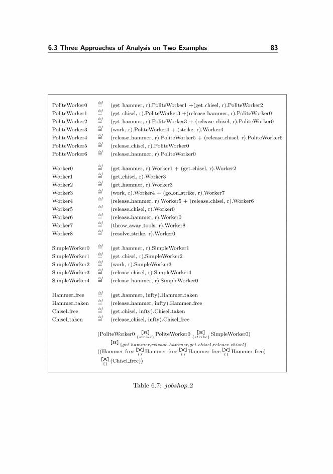
6.3 Three Approaches of Analysis on Two Examples 83
PoliteWorker0def= (get hammer, r).PoliteWorker1 +(get chisel, r).PoliteWorker2
PoliteWorker1def= (get chisel, r).PoliteWorker3 +(release hammer, r).PoliteWorker0
PoliteWorker2def= (get hammer, r).PoliteWorker3 + (release chisel, r).PoliteWorker0
PoliteWorker3def= (work, r).PoliteWorker4 + (strike, r).Worker4
PoliteWorker4def= (release hammer, r).PoliteWorker5 + (release chisel, r).PoliteWorker6
PoliteWorker5def= (release chisel, r).PoliteWorker0
PoliteWorker6def= (release hammer, r).PoliteWorker0
Worker0def= (get hammer, r).Worker1 + (get chisel, r).Worker2
Worker1def= (get chisel, r).Worker3
Worker2def= (get hammer, r).Worker3
Worker3def= (work, r).Worker4 + (go on strike, r).Worker7
Worker4def= (release hammer, r).Worker5 + (release chisel, r).Worker6
Worker5def= (release chisel, r).Worker0
Worker6def= (release hammer, r).Worker0
Worker7def= (throw away tools, r).Worker8
Worker8def= (resolve strike, r).Worker0
SimpleWorker0def= (get hammer, r).SimpleWorker1
SimpleWorker1def= (get chisel, r).SimpleWorker2
SimpleWorker2def= (work, r).SimpleWorker3
SimpleWorker3def= (release chisel, r).SimpleWorker4
SimpleWorker4def= (release hammer, r).SimpleWorker0
Hammer freedef= (get hammer, infty).Hammer taken
Hammer takendef= (release hammer, infty).Hammer free
Chisel freedef= (get chisel, infty).Chisel taken
Chisel takendef= (release chisel, infty).Chisel free
(PoliteWorker0 ��{strike}
PoliteWorker0 ��{strike}
SimpleWorker0)
�� {get hammer,release hammer,get chisel,release chisel}
((Hammer free ��{}
Hammer free ��{}
Hammer free ��{}
Hammer free)
��{}
(Chisel free))
Table 6.7: jobshop 2

84 Accelerate the Analysis
These two programs are much larger than the programs in the previous ex-amples. For each program we performed the original analysis, analysis basedon method 1 and analysis based on method 2 and build their correspondingautomatons.
The basic configuration of the computer performing the analysis(throughout thewhole thesis) is: Intel Pentium M processor 1.60GHz, 1.00GB of RAM and runson Microsoft Windows XP Professional Service Pack 2.
The results is shown in Table 6.8. It could be seen clearly that in both cases,methods 2 generates the automatons with least states and spends least time,while the original analysis consumes the maximum time among three analysisand also generates the number of states that higher than the others.
The accelerating rates between time used for running jobshop1 by method2 andoriginal analysis is:
r20 =4 hours 32 minutes 37 seconds
6 seconds= 2726
While the accelerating rates between time used for running jobshop1 by method1and original analysis is:
r10 =4 hours 32 minutes 37 seconds
1 minutes 1 second= 268
The accelerating rates between time used for running jobshop1 by method2 andmethod1 is:
r21 =1 minutes 1 seconds
6 seconds= 10
Obviously, the acceleration of the analysis works! Method 1 greatly improves theoriginal analysis(r10 = 258), the method 2 slightly improves the method1(r21 =
Program Item Original analysis Method1 Method2jobshop1 States of Automaton 1371 235 131
Time Cost 4 hours 1 minute 6 seconds32 minutes 1 second37 seconds
jobshop2 States of Automaton 557 117 66Time Cost 31 minutes 17 seconds 2 seconds
59 seconds
Table 6.8: Analysis results on jobshop1 and jobshop2

6.4 Discussion of method1 and method2 85
q_0
(<1,01>:<1,00>) q_2
(<2,01>:<1,00>)
q_3(<1,01>:<2,00>)
q_1(<2,01>:<2,00>)
<3,01>
<3,00>
<3,00>
<3,01>
Figure 6.5: Automaton built by original analysis
10) and lastly method2 improves the original analysis by 2726 times(r20 = 2726).The result from jobshop2 shows the similar conclusion and we will not explainit here.
6.4 Discussion of method1 and method2
We have seen that both method1 and method2 could increase the speed of theanalysis, nevertheless these two techniques hold essentially different character-istics from each other.
Since method2 is based on the development of method1, it inherits all featuresmethod1 have: both of them could collapse sequential processes conjointly co-operating on empty set. What is more, method 2 goes one step further thanmethod 1 on that it could collapse sequential processes conjointly cooperatingon non-empty set. Here we pinpoint that this extra feature the method2 ownswill potentially add more interactions (some actions are not allowed to cooperatewith each other based on the original semantics of the program, but method2might make them possible) to the automaton built by the original analysis. Incontract, method1 will not add more interactions(from the semantics point ofview) than the automaton built before.
Example 6.8 Let’s take the following program
let S , (g1, r1).S + (g2, r2).(p3, r3).Sin S00 ��
{g}S01
If we use original analysis, we will get an automaton shown in Figure 6.5. Thetable below shows the exposed actions corresponding to each state.

86 Accelerate the Analysis
q_0
(<1,0>:<1,0>)
q_1
(<1,0>:<2,0>)
q_2(<2,0>:<2,0>)
<3,0>
q_3(<1,0>:<2,0>)
q_5(<1,0>:<2,0>)
q_4
<3,0><3,0>
Figure 6.6: Automaton built by method2, round 4
q E[q]q0 ⊥Mex[(1, 00) 7→ 1, (2, 00) 7→ 1, (1, 01) 7→ 1, (2, 01) 7→ 1]
q1 ⊥Mex[(3, 00) 7→ 1, (3, 01) 7→ 1]
q2 ⊥Mex[(1, 00) 7→ 1, (2, 00) 7→ 1, (3, 01) 7→ 1]
q3 ⊥Mex[(1, 01) 7→ 1, (2, 01) 7→ 1, (3, 00) 7→ 1]
What we are interested in with this automaton is states q2 and q3, which are gen-erated by interaction < 1, 00 >:< 2, 01 > from q0, and interaction < 1, 01 >:<2, 00 > from q0. Take q2 for instance, the original analysis will ensure that(1,00) and (2,00) will not interact with each other, this is because that both ofthem are actions from the same sequential process which layered 00 and theyshould cooperate with actions from other layers but not themselves. The onlyenabled transition at q2 is (3,01). However, this is not the case in automatonbuilt by method2.
If we use the method2 to construct the automaton and keep using granularityfunction HLabex,>, the automaton will not terminate at all. Figure 6.6 showsthe automaton we get after the round 4 of execution of the worklist algorithmin Table 5.1. Notice that red edges marking with transition < 1, 0 >:< 2, 0 >in Figure 6.6 connect all blue nodes (q0, q1, q3, q5) together. If we compare tran-sitions in Figure 6.5, there is no similar structure, where the transition after< 1, 00 >:< 2, 01 > ( or < 1, 01 >:< 2, 00 >) will always come with an transi-tion < 3, 01 > (or < 3, 00 >). Lets take a look at the exposed actions of eachstate after executing round 4 by constructing the automaton with method2:

6.4 Discussion of method1 and method2 87
q E[q]q0 ⊥Mex[(1, 0) 7→ 2, (2, 0) 7→ 1]
q1 ⊥Mex[(1, 0) 7→ 1, (2, 0) 7→ 1, (3, 0) 7→ 1]
q2 ⊥Mex[(3, 0) 7→ 2]
q3 ⊥Mex[(1, 0) 7→ 1, (2, 0) 7→ 1, (3, 0) 7→ 2]
q4 ⊥Mex[(1, 0) 7→ 2, (2, 0) 7→ 2, (3, 0) 7→ 1]
q5 ⊥Mex[(1, 0) 7→ 1, (2, 0) 7→ 1, (3, 0) 7→ 3]
If we look closely at q1, we will find exposed actions including (1,0) and (2,0).This state is essentially the states of q2 and q3 in Fugure 6.5. The action(1,0) and (2,0) should come originally from the same sequential process butnow method2 can’t differentiate between them and will make a wrong judgementthat they are enabled! Thus the transition < 1, 0 >:< 2, 0 > that from q1 toq3 shouldn’t be there and it is the extra transition caused by method2. Thetransition from q3 and q5 is generated by the same reason. Furthermore , theoccurrence of exposed actions of (1,0) and (2,0) are all to be 1 in q1, q3 and q5,but the occurrence of exposed actions of (3,0) are gradually increased in thesestates. The automaton will follow this trend and build more extra states andtransitions if we didn’t terminate the constructing procedure by hand.
Method1 will not encounter the problem demonstrated in the above example,this is because all superfluous transitions made by method2 are actions cooper-ating within the same sequential components(due to the grouping). In method1,only sequential components cooperating on empty set will be grouped togetherand then there is no cooperation within the same sequential components.
In this sense, we say method1 doesn’t loose any precision of the original analysis,it just speed up the analysis by hiding information we don’t want to differentiate.However, to some extent, method2 will lose some precision from the originalanalysis. Even though it accelerate the analysis, it might built more interactionsand make over-approximation of the original analysis.
Anyway, there still exists situation where method2 will not lose any precisionfrom the original analysis: when there are same sequential processes conjointlycooperating on non-empty set, and all actions in this set only have maximumone occurrence in the sequential process, then the automaton we build will notencounter problem as shown in the above example and we still get a improvementof the speed without losing any precision.

88 Accelerate the Analysis
Example 6.9 For example, we define a sequential process S1 below:
S1 , (g, r).S2;S2 , (p, r).(h, r).S1;
Sequential process S1 doesn’t have two actions with the same type(g,p,h onlyoccur once) and then it is safe to group this kind of sequential process (S1)that cooperating on set containing action g, p, h. However, if we define anothersequential processes P1 below:
P1 , (g, r).P2;P2 , (p, r).(g, r).P1;
Sequential process P1 does have two actions with the same type(g occur twice)and then if we group this kind of sequential process (P1) that cooperating on setcontaining action g, we might lose precision and built more edges than we want.
The processes in Example 6.7, in Table 6.6 and Table 6.7 are all the cases thatcould safely use method2 for improving the speed of analysis without losing anyprecision from the original analysis.

Chapter 7
Deadlock Verification
In the previous chapters we have developed several static analysis techniques forPEPA. We are able to build up an automaton reflecting the interactions amongseveral PEPA processes. In this chapter, we are going to explore the deadlockproperty of PEPA program by our analysis, for answering the two questionsproposed in Chapter 1.
7.1 Deadlock of PEPA
In the operating system area, deadlock can be defined formally as follows [32]:
A set of processes are deadlocked if each process in the set is waitingfor an event that only another process in the set can cause.
Remember in PEPA, some actions in a sequential process can only be accom-plished when there exists another action in other sequential processes to coop-erate with.
Thus we say a program written by PEPA is deadlocked if each sequential processin the program is waiting for the actions required to cooperate, and only another
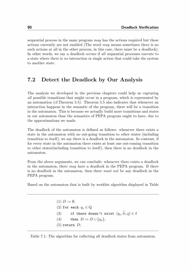
90 Deadlock Verification
sequential process in the same program may has the actions required but theseactions currently are not enabled (The word may means sometimes there is nosuch actions at all in the other process, in this case, there must be a deadlock).In other words, we say a deadlock occurs if all sequential processes execute toa state where there is no interaction or single action that could take the systemto another state.
7.2 Detect the Deadlock by Our Analysis
The analysis we developed in the previous chapters could help us capturingall possible transitions that might occur in a program, which is represented byan automation (cf.Theorem 5.5). Theorem 5.5 also indicates that whenever aninteraction happens in the semantic of the program, there will be a transitionin the automaton. This is because we actually build more transitions and statesin our automaton than the semantics of PEPA program ought to have, due tothe approximations we made.
The deadlock of the automaton is defined as follows: whenever there exists astate in the automaton with no out-going transition to other states (includingtransition to itself), we say there is a deadlock in the automaton. In contrast, iffor every state in the automaton there exists at least one out-coming transitionto other states(including transition to itself), then there is no deadlock in theautomaton.
From the above arguments, we can conclude: whenever there exists a deadlockin the automaton, there may have a deadlock in the PEPA program. If thereis no deadlock in the automaton, then there must not be any deadlock in thePEPA program.
Based on the automaton that is built by worklist algorithm displayed in Table
(1) D := ∅;(2) for each qs ∈ Q
(3) if there doesn’t exist (qs, ˜̀ı, q) ∈ δ
(4) then D := D ∪ {qs};(5) return D;
Table 7.1: The algorithm for collecting all deadlock states from automaton.

7.2 Detect the Deadlock by Our Analysis 91
5.1, we introduce another algorithm for collecting all deadlock states from theautomaton. The algorithm is displayed in Table 7.1. In the algorithm, D is aset that holds all deadlock states which are detected. The other variables justremain the same as before. Line(2)-Line(4) describe that we go through eachstate of the automaton and check whether the state has any out-going transition.If there doesn’t exist any such transition for a certain state, this state will beincluded in the set D.
Example 7.1 Let’s take the definition of the sequential process from Example2.1. Now we focus on two model components of the program as shown below inCase1 and Case2.
S , (g1, r1).(p2, r2).SQ , (g3, r3).(h4, r4).Q + (p5, r5).Q
Case1 : S00 ��{g,p,h}
Q01
Case2 : S00 ��{g,p,h}
Q01/h
q E[q] D = {q1}q0 ⊥Mex[(1, 00) 7→ 1, (3, 01) 7→ 1,
(5, 01) 7→ 1]
q1 ⊥Mex[(2, 00) 7→ 1, (4, 01) 7→ 1,
q E[q] D = ∅q0 ⊥Mex[(1, 00) 7→ 1, (3, 01) 7→ 1,
(5, 01) 7→ 1]
q1 ⊥Mex[(2, 00) 7→ 1, (4, 01) 7→ 1,
q2 ⊥Mex[(2, 00) 7→ 1, (3, 01) 7→ 1,
(5, 01) 7→ 1]
q_0 q_1(<3,01>:<1,00>)
Figure 7.1: The automaton of Case 1
q_0
q_1(<3,01>:<1,00>)
q_2
<4,01>
(<5,01>:<2,00>)
Figure 7.2: The automaton of Case 2
We construct two automatons shown in Figure 7.1 and Figure 7.2.
In Figure 7.1, the state q1 doesn’t have any out-going transition(D = {q1}), thisis because all the exposed actions in q1(p in process S and h in process Q) need tocooperate with their corresponding actions in the other sequential process. Sincethere isn’t any required actions available at that time, the program just comes toa deadlock.
In Figure 7.2, even though state q1 have the same exposed action as in Figure 7.1,the state q1 has one transition < 4, 01 > to q2. This is because the exposed actionh in process Q is hidden by the hidden set {h} and doesn’t need to cooperate

92 Deadlock Verification
with other actions. Furthermore, all states have out-going transitions to otherstates(D = ∅), so we can guarantee that there is no deadlock in this case.
For Case 1, we have found a possible deadlock by the deadlock collecting al-gorithm executing on our automaton where there is indeed a deadlock for thesemantic execution of the program. For Case 2, we don’t detect any deadlockfrom our automaton and we can guarantee that there is no deadlock in the pro-gram.
In the example above, it demonstrate clearly that our automaton could facilitateus finding deadlock or guarantee the absence of deadlocks in a given program.
In the mean time, it also shows us that our analysis is able to answer thequestion 1 introduced in Chapter 1: our analysis could verify whether the systempotentially have chance to go into the deadlock states.
7.3 Detect the Deadlock of Jobshop Examples
In this part, we are going to utilize our analysis to detect the deadlock in sev-eral variants of Milner’s process for a jobshop. Quite different from the simpleprograms presented above, they are programs far more complex and it is of-ten impossible for people to check manually. However, our analysis shows itscompetence in this scenario.
7.3.1 The deadlock path-finding algorithm
Before analyzing any jobshop examples, we introduce a simple path-finding al-gorithm, which could be used to find several paths from the initial state q0 toeach deadlock state of the automaton.
The algorithm applies Depth-First searching methodology to find the deadlockstates and will track each path leading to them. When traverse the graphof the automaton, we will not visit a non- deadlock state twice to guaranteethe termination of the algorithm. Actually, the algorithm only traverses theprogram tree once and complete the job.
This algorithm could help us find some paths on the way to deadlock state.However, we can’t guarantee any property of the paths we find: they are notnecessarily the shortest paths to the deadlock states, nor do the paths cover

7.3 Detect the Deadlock of Jobshop Examples 93
let Worker0 , (get hammer1, r).Worker1 + (get chisel2, r).Worker2;
Worker1 , (get chisel3, r).Worker3;
Worker2 , (get hammer4, r).Worker3;
Worker3 , (work5,r).Worker4;
Worker4 , (release hammer6, r).Worker5 +(release chisel7, r).Worker6;
Worker5 , (release chisel8,r).Worker0;
Worker6 , (release hammer9,r).Worker0;
Hammer free , (get hammer10, infty).Hammer taken;
Hammer taken , (release hammer11, infty).Hammer free;
Chisel free , (get chisel12, infty).Chisel taken;
Chisel taken , (release chisel13, infty).Chisel free;
in (Worker0000 ��{}
Worker0001)
�� {get hammer,release hammer,get chisel,release chisel}
(Hammer free010 ��{}
Chisel free011)
Table 7.2: jobshop 3
all possible routes to each state (sometimes finding all possible paths to eachdeadlock state is impossible because there often exists circle path in the graphof the automaton). The purpose of developing this algorithm is just to help usfind some paths leading to the deadlock states.
Here, we only presented the basic idea of the algorithm and will not make furtherdiscussion in the following subsections.
7.3.2 Analysis of the Jobshop3
Firstly, let’s take jobshop3 displayed in Table 7.2 as an example, where we addlabel to all sequential components and add layer to all model components.
7.3.2.1 Analysis by Method 1
From the characteristic of model components((Worker0 ��{}
Worker0)), we areable to choose method 1 and ignore the difference of them to accelerate analysisspeed. Using method 1, we obtain an automaton which is shown in Figure 7.3.
The automaton has 10 states, in which q4 is the deadlock state represented

94 Deadlock Verification
q_0
q_1
(<12,011>:<2,00>)
q_2(<10,010>:<1,00>) q_4
(<10,010>:<1,00>)
q_3(<10,010>:<4,00>)
(<12,011>:<2,00>)
(<12,011>:<3,00>)
q_5<5,00>
q_6(<11,010>:<6,00>)
q_7(<13,011>:<7,00>)
(<13,011>:<8,00>)
q_8(<10,010>:<1,00>)
(<11,010>:<9,00>)
q_9
(<12,011>:<2,00>)
(<13,011>:<8,00>)
(<11,010>:<9,00>)
Figure 7.3: Automaton of jobshop3 by method1
by a gold node. The red edges are two paths from the initial state q0 to thedeadlock state q4 computed by our path-finding algorithm. The path from q0
via q2 to q4 illustrates the case that if a worker(layered 00) gets a hammer andthen a worker(layered 00) gets a chisel, then there might be a deadlock state,while the path from q0 via q1 to q4 illustrates that picking up the tools in anopposite sequence might still lead to a deadlock state. However, just from theseoversimplified information it is not straightforward to guess why a deadlockexists. The worker0 defined in 7.3 only tells us a typical worker will alwayspickup two tools and then release them, in any order. The information obtainedfrom our deadlock paths seems to illustrate a case that the workers behaviorregularly!
7.3.2.2 Analysis by Original Method
Since we already know there might be a deadlock state from the result of Method1, now we will use the original analysis without ignoring any information andtry to distinguish the behavior of two workers. We want to find out what exactlywould happen when we go into a deadlock state!
We built the automaton shown in 7.4, which has 19 states. Two gold statesq6 and q8 are deadlock states. As before, deadlock paths found by our path-finding algorithm are represented by red edges in the figure. It can be easilyseen from the graph that the deadlock path q0 via q2 to q8 is not figured out byour path-finding algorithm, but some much longer paths are found, for example:q0, q1, q5, q9, q12, q16, q2, q8. This is due to the fact our algorithm bases on Depth-First searching methodology and will not revisit any non deadlock state.
Now we inspect some deadlock paths in the automaton. Take q0 via q1 to q6 forexample, the transitions during this paths explain clearly that worker layered000 first gets a chisel, and then worker layered 001 gets a hammer. And we start

7.3 Detect the Deadlock of Jobshop Examples 95
q_0
q_1(<12,011>:<2,000>)
q_2
(<12,011>:<2,001>)
q_3
(<10,010>:<1,000>)
q_4
(<10,010>:<1,001>)
q_5(<10,010>:<4,000>)
q_6(<10,010>:<1,001>)
q_7(<10,010>:<4,001>)
q_8(<10,010>:<1,000>)
(<12,011>:<3,000>)
(<12,011>:<2,001>)
(<12,011>:<2,000>)
(<12,011>:<3,001>)
q_9
<5,000>
q_10
<5,001>
q_11(<11,010>:<6,000>)
q_12
(<13,011>:<7,000>)
q_13(<13,011>:<7,001>)
q_14
(<11,010>:<6,001>)
(<13,011>:<8,000>)
q_15(<10,010>:<1,001>)
(<11,010>:<9,000>)q_16
(<12,011>:<2,001>)(<11,010>:<9,001>)
q_17(<12,011>:<2,000>)
(<13,011>:<8,001>)q_18
(<10,010>:<1,000>)
(<13,011>:<8,000>)
(<11,010>:<9,000>)
(<11,010>:<9,001>)
(<13,011>:<8,001>)
Figure 7.4: Automaton of jobshop3 by original analysis
the system with one hammer and one chisel. Now we could know what exactlyhappen when we go into a deadlock state: each worker gets a tool and waits forthe other one to release the tool!
Up to now, we have shown that the two analysis methods indeed could helpus study the deadlock property of the program. Method1 is much faster butcan’t give us all information we want, while the original analysis needs morecomputing power but is very precise and provides us with more information.
This example also shows us our analysis not only could answer question 1, it alsobe able to answer the question 2 introduced in Chapter 1: our analysis couldtell that if there exist deadlock states, how the system behaves before reachingthose states.
7.3.3 Analysis of the Jobshop1 and Jobshop2
In Section 6.3, we have already introduced jobshop1(cf. Table 6.6) and job-shop2(cf. Table 6.7) and built automatons in three approaches for each ofthem. Now we study the deadlock property of these two programs from threeapproaches.
Table 7.3 lists the results produced by the deadlock states collecting algorithm

96 Deadlock Verification
Program Item Original analysis Method1 Method2jobshop1 Overall States 1371 235 131
Time Cost 4 hours 1 minute 6 seconds32 minutes 1 second37 seconds
Deadlock States {q 1359, {q 224, {q 126,q 1361, q 225, q 130}q 1370} q 234}
jobshop2 Overall States 557 117 66Time Cost 31 minutes 17 seconds 2 seconds
59 secondsDeadlock States ∅ ∅ ∅
Table 7.3: Deadlock results on jobshop1 and jobshop2
shown in Table 7.1, and it also includes the result from Table 6.8.
For jobshop1, all three analyses have detected out deadlock states in the au-tomaton. While for jobshop2, nothing has been reported from each analysis.We conclude that to check the existence of deadlock in an automaton, method1 or method 2 are good choices since they are much faster and still correct.However, to understand how comes the deadlocks, we should try to proceed theoriginal analysis, even though sometimes it costs too much time and becomesimpossible.
7.3.4 Analysis of Jobshop4-Jobshop11
Now we are going to analyze jobshop4 to jobshop11 shown in Appendix A. Sincemost of them are very complex and they all meet the condition of method 1, wejust use method 1 to analyze and verify these programs. The results are listedin Table 7.4.
7.3.4.1 Jobshop4 and Jobshop5
Our analysis shows that jobshop4 and jobshop5 both may have deadlock states,which is easily understood: the worker0 will pick up hammer and chisel to work,but its behavior determines that sometimes he will throw away tools. When itcomes to a state that all tools have been thrown away by worker0, the deadlockoccurs since they can’t pick up tools anymore.

7.3 Detect the Deadlock of Jobshop Examples 97
Program Overall States Deadlock States Time Costjobshop4 87 {q 49, q 77} 2 secondsjobshop5 868 {q 596, q 771, q 841} 37 minutes 29 secondsjobshop6 28 ∅ less then 1 secondjobshop7 10 ∅ less then 1 secondjobshop8 122 ∅ 10 secondsjobshop9 164 ∅ 21 secondsjobshop10 1199 {q 256} 3 hours and 34 secondsjobshop11 1672 ∅ 10 hours 51 minutes
38 seconds
Table 7.4: Deadlock results on jobshop4 to jobshop11 by method1
7.3.4.2 Jobshop6 to Jobshop9
Jobshop6 to Jobshop9 doesn’t show any deadlock states by our analysis. Theycontain two kinds of workers:
• The worker0 who won’t throw away tools. If there are enough tools, theywill work continually without stopping.(No matter how many tools areavailable at the start of the program, if a program contains a worker0 thatbehaves as the one (could throw away tools) in jobshop4 and jobhshop5,the program will definitely go to the deadlock state)
• The politework0 who doesn’t necessarily request for two tools at one time.If there exists one tool(no matter it is a hammer or a chisel)in the system,the politework0 will always be satisfied.
From the description above, these two workers will not throw away tools. Thusif we start the system with enough tools, all workers will be satisfied. Sincewe don’t get any deadlock from the report of our analysis, there must be nodeadlock. Thus we believe that the tools are enough for the workers in theseprograms.
7.3.4.3 Jobshop10 and Jobshop11
Jobshop10 and jobshop11 are both larger examples. One contains 1199 statesand the other contains 1672 states(by method 1)! There are two kinds of work-ers: LeftHandedWorker0 and RightHandedWorker0, characterized by pickingup hammer first and picking up chisel respectively.

98 Deadlock Verification
One deadlock state has been detected in jobshop10, showing that there may bea deadlock. After carefully considering some extreme cases, we believe thereshould be one deadlock: image that if all four LeftHandedWorker0 pick up allfour hammers, while all four RightHandedWorker0 pick up all four chisels, allworkers will be stuck, which comes to the deadlock state.
There is no deadlock state in jobshop11, reported from our analysis, and theremust not have deadlock. The only difference from jobshop11 and jobhshop10is: in jobhsop11 the system starts with five hammers instead of four. Since theRightHandedWorker0 will still get hammer even if all LeftHandedWorker0 havealready picked their hammers. It seems that at least one RightHandedWorker0will always be satisfied, which should be the reason the program doesn’t havedeadlock state.
Through jobshop4 to jobshop11, we just verify the deadlock property for eachof them by the deadlock state collecting algorithm. Based on the results wegot, some speculation on the result are presented, and we try to explain whythere exists a deadlock or why not. Instead, we could also use path-findingalgorithm to show the path leading to each deadlock state, and based on thoseinformation and we can make a much more accurate explanation of the result.We didn’t show the result generated by path-finding algorithm since in some ofthese examples, the number of transitions along these pathes are quite huge andit doesn’t worth showing them all. Please refer to the CD attached with thisthesis to see all results generated by our analysis from the jobshop1-11.

Chapter 8
Conclusion
The initial goal of the project is to develop static analysis and answer the twoquestions proposed in Chapter 1:
• Does the system potentially have chance to go into the deadlock states?
• If there exist deadlock states, how does the system behave before reachingthose states?
8.1 Achievement
To solve these questions, we developed our analysis and constructed an automa-ton to capture the control structure of the PEPA program, which is presentedfrom Chapter 2 to Chapter 5. The automaton could faithfully reflect the in-teractions by transitions, while track the configuration of their exposed actionsby states. Once we get this automaton, the questions above could be easilysolved, as shown in Chapter 7. The initial version of the analysis developedare very precise that could be used to proceed exhaustive study of the systembehavior. However, sometimes it is not necessary to be that accurate. Thus wedeveloped two methods in Chapter 6 to lower the precision of the analysis, and

100 Conclusion
these modification would generate much more succinct automatons in a shortertime.
Even though our work adopts the approach originally developed for analyzingCCS [16, 15], it owns its unique feature. In [16, 15], the authors annotate labelto the CCS program. Not only did we annotate label, but also annotate layerto PEPA program. Consequently, we could do a much more precise approxima-tion than theirs could do. Simply speaking, their analysis is quite similar to themethod 1 and method 2 we proposed and the common characteristic of them isthat they don’t differentiate sequential processes with the same name. In con-trast, our original analysis is able to distinguish those processes. Subsequently,our original analysis is much more accurate and informative, and could capturethe controlstructure of the program much better.
8.2 Limitation
Our analysis could only handle PEPA program in a certain scale, depending onthe approach we chose. The original analysis could get the most precise resultcomparing two other methods, however it could only handle PEPA program inthe least scale. Method 2 and Method 1 could handle the program with a muchlarger scale, as long as the program fulfills certain requirements.
However, from Table 7.4, we could see that even by Method 1, constructing theautomaton of jobshop11 costs 10 hours 51 minutes 38 seconds, which is not ashort time indeed. It can be imagined that our program can’t efficiently handlean arbitrary large program. In other words, our analysis suffers the so-calledstate explosion problem[33].
8.3 Future Work
Due to the restricted time schedule of the project, there are some tasks worthdoing in the future.
8.3.1 Prove the Conjectures
The formal proof for one of the assumption in Theorem 5.5 is not completelydone yet, we only give several steps of the proof in this thesis. We believe

8.3 Future Work 101
this assumption could be proved after finding more invariants in the enabledfunction and all its auxiliary functions.
Moreover, under certain condition(the PEPA program is written in the styleof program (b) in Subsection 5.5), we hypothesize that our original analysisperforms the approximation of system behavior with one hundred percent pre-cision. In other words, we believe our analysis could faithfully capture thesystem behavior exactly, and there will be no more edges in the automaton webuilt than the transitions in the semantic world. We believe this conjecturecould be formally proven to be true.
8.3.2 Optimize the Path-finding Algorithm
In Chapter 7, we have discussed that we developed a path-finding algorithmto find paths leading to deadlock states. We also admit that this algorithmcan’t guarantee the found paths hold any property. Thus, we could change thisalgorithm to show much more interesting paths for people to study the systemproperty, e.g. algorithm of finding the shortest path from the initial state to adeadlock state (Dijkstra’s algorithm [14]). Basically, different algorithms couldgenerate pathes with different properties. The various algorithms could be freelypicked up from the graph theory.
8.3.3 Integrate activity rate into the Analysis
In PEPA, an activity a is defined as a pair (α, r) where α is the action typeand r is the activity rate that indicates the duration of this activity. In ouranalysis, we only deal with activity type α, which will directly be influenced bycooperation or hiding combinators, telling whether the activity should proceedor not. For the activity rate r, we just get rid of it. The automaton we obtainedin this way could answer the two questions proposed in Chapter 1, however,it can’t answer other questions like: in what probability does the system enterinto a certain state? In other words, our analysis could capture all transitionsin the system, however, it doesn’t keep track of any properties(the rate r) of thetransitions.
Thus, in order to get a much more comprehensive understanding of the systembehavior, we shall integrate the activity rate into the analysis in an appropriateway. For example, we shall redefine a set of functions like : Ep
? ,Gp? etc, and put
r into them according to the semantics of PEPA shown in Table 2.1. And thisdirection definitely worth further investigation.

102 Conclusion

Appendix A
The Syntax of Jobshop 4 - 11

104 The Syntax of Jobshop 4 - 11
Worker0def= (get hammer, r).Worker1 + (get chisel, r).Worker2
Worker1def= (get chisel, r).Worker3
Worker2def= (get hammer, r).Worker3
Worker3def= (work, r).Worker4 + (go on strike, r).Worker7
Worker4def= (release hammer, r).Worker5 + (release chisel, r).Worker6
Worker5def= (release chisel, r).Worker0
Worker6def= (release hammer, r).Worker0
Worker7def= (throw away tools, r).Worker8
Worker8def= (resolve strike, r).Worker0
Hammer freedef= (get hammer, infty).Hammer taken
Hammer takendef= (release hammer, infty).Hammer free
Chisel freedef= (get chisel, infty).Chisel taken
Chisel takendef= (release chisel, infty).Chisel free
(Worker0 ��{}
Worker0 ��{}
Worker0)
�� {get hammer,release hammer,get chisel,release chisel}
((Hammer free ��{}
Hammer free)
��{}
(Chisel free ��{}
Chisel free))
Table A.1: jobshop 4

105
Worker0def= (get hammer, r).Worker1 + (get chisel, r).Worker2
Worker1def= (get chisel, r).Worker3
Worker2def= (get hammer, r).Worker3
Worker3def= (work, r).Worker4 + (go on strike, r).Worker7
Worker4def= (release hammer, r).Worker5 + (release chisel, r).Worker6
Worker5def= (release chisel, r).Worker0
Worker6def= (release hammer, r).Worker0
Worker7def= (throw away tools, r).Worker8
Worker8def= (resolve strike, r).Worker0
Hammer freedef= (get hammer, infty).Hammer taken
Hammer takendef= (release hammer, infty).Hammer free
Chisel freedef= (get chisel, infty).Chisel taken
Chisel takendef= (release chisel, infty).Chisel free
(Worker0 ��{}
Worker0 ��{}
Worker0 ��{}
Worker0)
�� {get hammer,release hammer,get chisel,release chisel}
((Hammer free ��{}
Hammer free ��{}
Hammer free ��{}
Hammer free)
��{}
(Chisel free ��{}
Chisel free ��{}
Chisel free ��{}
Chisel free))
Table A.2: jobshop 5
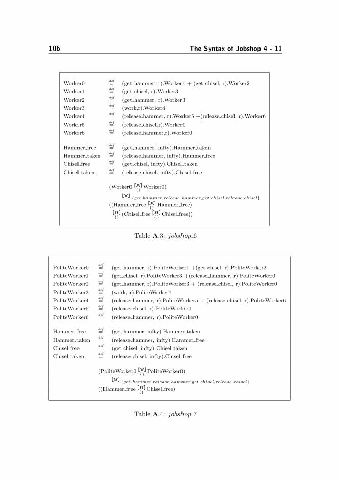
106 The Syntax of Jobshop 4 - 11
Worker0def= (get hammer, r).Worker1 + (get chisel, r).Worker2
Worker1def= (get chisel, r).Worker3
Worker2def= (get hammer, r).Worker3
Worker3def= (work,r).Worker4
Worker4def= (release hammer, r).Worker5 +(release chisel, r).Worker6
Worker5def= (release chisel,r).Worker0
Worker6def= (release hammer,r).Worker0
Hammer freedef= (get hammer, infty).Hammer taken
Hammer takendef= (release hammer, infty).Hammer free
Chisel freedef= (get chisel, infty).Chisel taken
Chisel takendef= (release chisel, infty).Chisel free
(Worker0 ��{}
Worker0)
�� {get hammer,release hammer,get chisel,release chisel}
((Hammer free ��{}
Hammer free)
��{}
(Chisel free ��{}
Chisel free))
Table A.3: jobshop 6
PoliteWorker0def= (get hammer, r).PoliteWorker1 +(get chisel, r).PoliteWorker2
PoliteWorker1def= (get chisel, r).PoliteWorker3 +(release hammer, r).PoliteWorker0
PoliteWorker2def= (get hammer, r).PoliteWorker3 + (release chisel, r).PoliteWorker0
PoliteWorker3def= (work, r).PoliteWorker4
PoliteWorker4def= (release hammer, r).PoliteWorker5 + (release chisel, r).PoliteWorker6
PoliteWorker5def= (release chisel, r).PoliteWorker0
PoliteWorker6def= (release hammer, r).PoliteWorker0
Hammer freedef= (get hammer, infty).Hammer taken
Hammer takendef= (release hammer, infty).Hammer free
Chisel freedef= (get chisel, infty).Chisel taken
Chisel takendef= (release chisel, infty).Chisel free
(PoliteWorker0 ��{}
PoliteWorker0)
�� {get hammer,release hammer,get chisel,release chisel}
((Hammer free ��{}
Chisel free)
Table A.4: jobshop 7

107
Worker0def= (get hammer, r).Worker1 + (get chisel, r).Worker2
Worker1def= (get chisel, r).Worker3
Worker2def= (get hammer, r).Worker3
Worker3def= (work,r).Worker4
Worker4def= (release hammer, r).Worker5 +(release chisel, r).Worker6
Worker5def= (release chisel,r).Worker0
Worker6def= (release hammer,r).Worker0
PoliteWorker0def= (get hammer, r).PoliteWorker1 +(get chisel, r).PoliteWorker2
PoliteWorker1def= (get chisel, r).PoliteWorker3 +(release hammer, r).PoliteWorker0
PoliteWorker2def= (get hammer, r).PoliteWorker3 + (release chisel, r).PoliteWorker0
PoliteWorker3def= (work, r).PoliteWorker4
PoliteWorker4def= (release hammer, r).PoliteWorker5 + (release chisel, r).PoliteWorker6
PoliteWorker5def= (release chisel, r).PoliteWorker0
PoliteWorker6def= (release hammer, r).PoliteWorker0
Hammer freedef= (get hammer, infty).Hammer taken
Hammer takendef= (release hammer, infty).Hammer free
Chisel freedef= (get chisel, infty).Chisel taken
Chisel takendef= (release chisel, infty).Chisel free
(Worker0 ��{}
Worker0 ��{}
PoliteWorker0)
�� {get hammer,release hammer,get chisel,release chisel}
((Hammer free ��{}
Hammer free)
��{}
(Chisel free ��{}
Chisel free))
Table A.5: jobshop 8
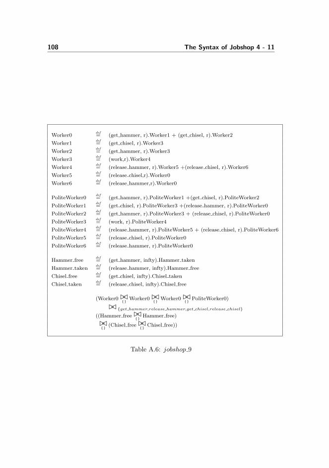
108 The Syntax of Jobshop 4 - 11
Worker0def= (get hammer, r).Worker1 + (get chisel, r).Worker2
Worker1def= (get chisel, r).Worker3
Worker2def= (get hammer, r).Worker3
Worker3def= (work,r).Worker4
Worker4def= (release hammer, r).Worker5 +(release chisel, r).Worker6
Worker5def= (release chisel,r).Worker0
Worker6def= (release hammer,r).Worker0
PoliteWorker0def= (get hammer, r).PoliteWorker1 +(get chisel, r).PoliteWorker2
PoliteWorker1def= (get chisel, r).PoliteWorker3 +(release hammer, r).PoliteWorker0
PoliteWorker2def= (get hammer, r).PoliteWorker3 + (release chisel, r).PoliteWorker0
PoliteWorker3def= (work, r).PoliteWorker4
PoliteWorker4def= (release hammer, r).PoliteWorker5 + (release chisel, r).PoliteWorker6
PoliteWorker5def= (release chisel, r).PoliteWorker0
PoliteWorker6def= (release hammer, r).PoliteWorker0
Hammer freedef= (get hammer, infty).Hammer taken
Hammer takendef= (release hammer, infty).Hammer free
Chisel freedef= (get chisel, infty).Chisel taken
Chisel takendef= (release chisel, infty).Chisel free
(Worker0 ��{}
Worker0 ��{}
Worker0 ��{}
PoliteWorker0)
�� {get hammer,release hammer,get chisel,release chisel}
((Hammer free ��{}
Hammer free)
��{}
(Chisel free ��{}
Chisel free))
Table A.6: jobshop 9

109
LeftHandedWorker0def= (get hammer, r).LeftHandedWorker1
LeftHandedWorker1def= (get chisel, r).LeftHandedWorker2
LeftHandedWorker2def= (work, r).LeftHandedWorker3
LeftHandedWorker3def= (release chisel, r).LeftHandedWorker4
LeftHandedWorker4def= (release hammer, r).LeftHandedWorker0
RightHandedWorker0def= (get chisel, r).RightHandedWorker1
RightHandedWorker1def= (get hammer, r).RightHandedWorker2
RightHandedWorker2def= (work, r).RightHandedWorker3
RightHandedWorker3def= (release hammer, r).RightHandedWorker4
RightHandedWorker4def= (release chisel, r).RightHandedWorker0
Hammer freedef= (get hammer, infty).Hammer taken
Hammer takendef= (release hammer, infty).Hammer free
Chisel freedef= (get chisel, infty).Chisel taken
Chisel takendef= (release chisel, infty).Chisel free
((LeftHandedWorker0 ��{}
LeftHandedWorker0 ��{}
LeftHandedWorker0
��{}
LeftHandedWorker0) ��{}
(RightHandedWorker0 ��{}
RightHandedWorker0 ��{}
RightHandedWorker0
��{}
RightHandedWorker0))
�� {get hammer,release hammer,get chisel,release chisel}
((Hammer free ��{}
Hammer free ��{}
Hammer free ��{}
Hammer free)
��{}
(Chisel free ��{}
Chisel free ��{}
Chisel free ��{}
Chisel free))
Table A.7: jobshop 10

110 The Syntax of Jobshop 4 - 11
LeftHandedWorker0def= (get hammer, r).LeftHandedWorker1
LeftHandedWorker1def= (get chisel, r).LeftHandedWorker2
LeftHandedWorker2def= (work, r).LeftHandedWorker3
LeftHandedWorker3def= (release chisel, r).LeftHandedWorker4
LeftHandedWorker4def= (release hammer, r).LeftHandedWorker0
RightHandedWorker0def= (get chisel, r).RightHandedWorker1
RightHandedWorker1def= (get hammer, r).RightHandedWorker2
RightHandedWorker2def= (work, r).RightHandedWorker3
RightHandedWorker3def= (release hammer, r).RightHandedWorker4
RightHandedWorker4def= (release chisel, r).RightHandedWorker0
Hammer freedef= (get hammer, infty).Hammer taken
Hammer takendef= (release hammer, infty).Hammer free
Chisel freedef= (get chisel, infty).Chisel taken
Chisel takendef= (release chisel, infty).Chisel free
((LeftHandedWorker0 ��{}
LeftHandedWorker0 ��{}
LeftHandedWorker0
��{}
LeftHandedWorker0) ��{}
(RightHandedWorker0 ��{}
RightHandedWorker0 ��{}
RightHandedWorker0
��{}
RightHandedWorker0))
�� {get hammer,release hammer,get chisel,release chisel}
((Hammer free ��{}
Hammer free ��{}
Hammer free ��{}
Hammer free ��{}
Hammer free)
��{}
(Chisel free ��{}
Chisel free ��{}
Chisel free ��{}
Chisel free))
Table A.8: jobshop 11

Appendix B
Design and Demonstration ofthe Tool
In this part, we will first give a short description of the tool we designed forstatic analysis of PEPA. Later we will show a concrete example of using thetool.
The overall procedure of utilizing our tool with other auxiliary software isdemonstrated in Figure B.1. From the figure, it is seen that our tool takesa plain-text PEPA file and output the result into two files:
• One file contains the important datastructure generated during the an-alyzing procedure, text representation of the automaton in the form asintroduced at start of Chapter 5, as well as the information of all deadlockstates that has been found;
• The other one contains the text representation of the automaton whichfollows the syntax of dot language [17, 4]. The dot format file could beinput into the dot tool(one part of the the open source graphic visualiza-tion software Graphviz [1]), from which a graphic representation of theautomaton could be generated.
Our tool is developed under Java language and contains two main parts: the

112 Design and Demonstration of the Tool
PEPA File
(Based on Concrete Syntax of PEPA
Language)
Parser(Build by ANTLR
Parser Generator)---Front-end
Intermediate Representation of
the PEPA program
The Analyzer(Core Program)---
Back-end
Dot File
( Intermediate representation of the automaton, based on
The syntax of Dot Language)
Analysis Result File
(1.Important data structure of the
analyzing procedure,2. Intermediate
representation of the automaton,
3. Deadlock Report)
Dot Tool(Graph Visualization
Software)
PS File
(Graphic representation of the
automaton)
Our Tool
Figure B.1: The Workflow of the Static Analysis
front-end, a parser; the back-end, the core program. We will introduce them inthe following subsections.

B.1 The Parser 113
B.1 The Parser
The parser could transform plain-text PEPA programs into the intermediate rep-resentations that are ready for the back-end program to work on, implementedusing Antlr [2], an open source parser generating tool. Here the plain-text PEPAis written in concrete syntax of PEPA. The reason to introduce this new syntaxis that the mathematical notation of PEPA introduced in Chapter 2.1 is reallyhard to input into the plain-text file.
Refering to some other concrete syntaxes of PEPA [30, 18, 19], we developed ourown syntax more or less the same as theirs. The only difference is we get rid ofthe rate initialization at the front of the program (such as r1 = 1; r2 = 5; · · · ),since our static analysis doesn’t take care of rate. Most of the combinatorsremain the same as displayed in Chapter 2.1, except for the cooperation combi-nator: e.g. S ��
{g,p}Q would be transformed into S < g, p > Q. The program will
start with the sequential component definition that contains one or more se-quential components, separated by semicolon, with model component definitionbeing the following part for further processing.
Example B.1 Let’s see how we transform a program written in mathematicsyntax into our new concrete syntax. Figure B.1 shows jobshop3 in originalmathematic notation. After the transformation, it becomes the program in Fig-ure B.2, which could be directly taken into our parser for further processing.
B.2 The Analyzer
The analyzer is the core part of our tool which takes the intermediate represen-tation of the PEPA program as input, and after finishing the computation, itoutputs the analysis result into two files. The analyzer implements the worklistalgorithm, all its auxiliary functions, and functions related to deadlock detectingand displaying, which are well defined through Chapter 3 to Chapter 7. Herewe won’t dig into any details, please refer to the source code that included inthe Appendix CD.
We thoroughly tested our tool, using Junit[3], an open source unit-testing frame-work for java. The test covers most significant classes and methods, and willsignificantly ensure the correctness of our design and implementation.
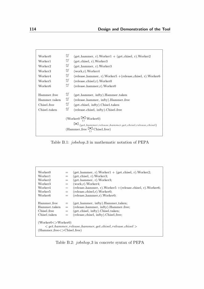
114 Design and Demonstration of the Tool
Worker0def= (get hammer, r).Worker1 + (get chisel, r).Worker2
Worker1def= (get chisel, r).Worker3
Worker2def= (get hammer, r).Worker3
Worker3def= (work,r).Worker4
Worker4def= (release hammer, r).Worker5 +(release chisel, r).Worker6
Worker5def= (release chisel,r).Worker0
Worker6def= (release hammer,r).Worker0
Hammer freedef= (get hammer, infty).Hammer taken
Hammer takendef= (release hammer, infty).Hammer free
Chisel freedef= (get chisel, infty).Chisel taken
Chisel takendef= (release chisel, infty).Chisel free
(Worker0 ��{}
Worker0)
�� {get hammer,release hammer,get chisel,release chisel}
(Hammer free ��{}
Chisel free)
Table B.1: jobshop 3 in mathematic notation of PEPA
Worker0 = (get hammer, r).Worker1 + (get chisel, r).Worker2;Worker1 = (get chisel, r).Worker3;Worker2 = (get hammer, r).Worker3;Worker3 = (work,r).Worker4;Worker4 = (release hammer, r).Worker5 +(release chisel, r).Worker6;Worker5 = (release chisel,r).Worker0;Worker6 = (release hammer,r).Worker0;
Hammer free = (get hammer, infty).Hammer taken;Hammer taken = (release hammer, infty).Hammer free;Chisel free = (get chisel, infty).Chisel taken;Chisel taken = (release chisel, infty).Chisel free;
(Worker0<>Worker0)< get hammer, release hammer, get chisel, release chisel >
(Hammer free<>Chisel free)
Table B.2: jobshop 3 in concrete syntax of PEPA

B.3 A Guide for Using the Tool through an Example 115
B.3 A Guide for Using the Tool through an Ex-ample
In order to use the tool, the standard Java Runtime Environment should be setup appropriate. In addition, we also need to put antlr package (antlr.jar) to theright class path. If we want to see the graph representation of the result, theGraphviz package should also be installed. Once we set up the environment, wecould use the tool to analyze PEPA program.
An Example
Here we demonstrate the tool through an example. Suppose the program weplan to analyze is stored in jobshop3.txt, with the content shown in Table B.2.
The Input
To start the program, type
java -classpath PEPATool.jar automaton.Automaton jobshop3.txt -v2 -pt -kn
In this command, PEPATool.jar contains all classes relevant to our tool, an-tomaton.Automaton is the main entry of the tool, jobshop3.txt is the PEPA filewe are going to analyze. The parameters afterwards could control the tool tobehave differently.
• -v: controls the version of the analysis. -v1 means using the originalanalysis; -v2 means using method 1 for accelerating the analysis; -v3 meansusing method 2 for accelerating the analysis.
• -p: controls graph output. -pt means to draw the graph while -pf meansno.
• -k: controls the granularity function of the analysis. -kn means k = >,-k0 means k = 0, -k1 means k = 1, etc.
If omit any number of these three parameters, the default setting is: -v2 -pf -kn.
In this example, we choose to use version 2(method1) with k = >. The graphwould be automatically drawn by the tool.
The Output

116 Design and Demonstration of the Tool
We will obtain the follow files: jobshop3 Result.txt (cf.Appendix B.4.1), job-shop3.dot (cf.Appendix B.4.2), and jobshop3.ps (cf.Appendix B.4.3).
Here jobshop3 Result.txt is the analysis result. jobshop3.dot is the automatonwith dot format. jobshop3.ps is graphic representation of the automaton drawnfrom jobshop3.dot.
B.4 Analysis Results
B.4.1 jobshop3 Result.txt
-----------------------------------------------------------------------Initially the program is....
Worker0=(<get_hammer,r>_0.Worker1+<get_chisel,r>_0.Worker2);Worker1=<get_chisel,r>_0.Worker3; Worker2=<get_hammer,r>_0.Worker3;Worker3=<work,r>_0.Worker4;Worker4=(<release_hammer,r>_0.Worker5+<release_chisel,r>_0.Worker6);Worker5=<release_chisel,r>_0.Worker0;Worker6=<release_hammer,r>_0.Worker0;Hammer_free=<get_hammer,infty>_0.Hammer_taken;Hammer_taken=<release_hammer,infty>_0.Hammer_free;Chisel_free=<get_chisel,infty>_0.Chisel_taken;Chisel_taken=<release_chisel,infty>_0.Chisel_free;((Worker0[]^1<>Worker0[]^1)^1<release_hammer,get_chisel,release_chisel,
get_hammer>(Hammer_free[]^1<>Chisel_free[]^1)^1)^1-----------------------------------------------------------------------The Simplified Program is:
Worker0=(<get_hammer,r>_1.Worker1+<get_chisel,r>_2.Worker2);Worker1=<get_chisel,r>_3.Worker3; Worker2=<get_hammer,r>_4.Worker3;Worker3=<work,r>_5.Worker4;Worker4=(<release_hammer,r>_6.Worker5+<release_chisel,r>_7.Worker6);Worker5=<release_chisel,r>_8.Worker0;Worker6=<release_hammer,r>_9.Worker0;Hammer_free=<get_hammer,infty>_10.Hammer_taken;Hammer_taken=<release_hammer,infty>_11.Hammer_free;Chisel_free=<get_chisel,infty>_12.Chisel_taken;Chisel_taken=<release_chisel,infty>_13.Chisel_free;(Worker0[]^2<release_hammer,get_chisel,release_chisel,get_hammer>

B.4 Analysis Results 117
(Hammer_free[]^1<>Chisel_free[]^1)^1)^1---------------------------------------------------------------------Important Data of the program, for constructing Automaton:
YEx: <12,011>={get_chisel,[0],[],null,false,}<13,011>={release_chisel,[0],[],null,false,}<10,010>={get_hammer,[0],[],null,false,}<11,010>={release_hammer,[0],[],null,false,}<1,00>={get_hammer,[0],[],null,false,}<2,00>={get_chisel,[0],[],null,false,}<3,00>={get_chisel,[0],[],null,false,}<4,00>={get_hammer,[0],[],null,false,}<5,00>={work,[],[],null,false,}<6,00>={release_hammer,[0],[],null,false,}<7,00>={release_chisel,[0],[],null,false,}<8,00>={release_chisel,[0],[],null,false,}<9,00>={release_hammer,[0],[],null,false,}
EEx: {<12,011>=1, <13,011>=0, <10,010>=1, <11,010>=0, <1,00>=2,<2,00>=2, <3,00>=0, <4,00>=0, <5,00>=0, <6,00>=0, <7,00>=0,<8,00>=0, <9,00>=0}
GEx: <12,011>={<12,011>=0, <13,011>=1, <10,010>=0, <11,010>=0,<1,00>=0, <2,00>=0, <3,00>=0, <4,00>=0, <5,00>=0, <6,00>=0,<7,00>=0, <8,00>=0, <9,00>=0}
<13,011>={<12,011>=1, <13,011>=0, <10,010>=0, <11,010>=0, <1,00>=0,<2,00>=0, <3,00>=0, <4,00>=0, <5,00>=0, <6,00>=0, <7,00>=0,<8,00>=0, <9,00>=0}
<10,010>={<12,011>=0, <13,011>=0, <10,010>=0, <11,010>=1, <1,00>=0,<2,00>=0, <3,00>=0, <4,00>=0, <5,00>=0, <6,00>=0, <7,00>=0,<8,00>=0, <9,00>=0}
<11,010>={<12,011>=0, <13,011>=0, <10,010>=1, <11,010>=0, <1,00>=0,<2,00>=0, <3,00>=0, <4,00>=0, <5,00>=0, <6,00>=0, <7,00>=0,<8,00>=0, <9,00>=0}
<1,00>={<12,011>=0, <13,011>=0, <10,010>=0, <11,010>=0, <1,00>=0,<2,00>=0, <3,00>=1, <4,00>=0, <5,00>=0, <6,00>=0, <7,00>=0,<8,00>=0, <9,00>=0}
<2,00>={<12,011>=0, <13,011>=0, <10,010>=0, <11,010>=0, <1,00>=0,<2,00>=0, <3,00>=0, <4,00>=1, <5,00>=0, <6,00>=0, <7,00>=0,

118 Design and Demonstration of the Tool
<8,00>=0, <9,00>=0}
<3,00>={<12,011>=0, <13,011>=0, <10,010>=0, <11,010>=0, <1,00>=0,<2,00>=0, <3,00>=0, <4,00>=0, <5,00>=1, <6,00>=0, <7,00>=0,<8,00>=0, <9,00>=0}
<4,00>={<12,011>=0, <13,011>=0, <10,010>=0, <11,010>=0, <1,00>=0,<2,00>=0, <3,00>=0, <4,00>=0, <5,00>=1, <6,00>=0, <7,00>=0,<8,00>=0, <9,00>=0}
<5,00>={<12,011>=0, <13,011>=0, <10,010>=0, <11,010>=0, <1,00>=0,<2,00>=0, <3,00>=0, <4,00>=0, <5,00>=0, <6,00>=1, <7,00>=1,<8,00>=0, <9,00>=0}
<6,00>={<12,011>=0, <13,011>=0, <10,010>=0, <11,010>=0, <1,00>=0,<2,00>=0, <3,00>=0, <4,00>=0, <5,00>=0, <6,00>=0, <7,00>=0,<8,00>=1, <9,00>=0}
<7,00>={<12,011>=0, <13,011>=0, <10,010>=0, <11,010>=0, <1,00>=0,<2,00>=0, <3,00>=0, <4,00>=0, <5,00>=0, <6,00>=0, <7,00>=0,<8,00>=0, <9,00>=1}
<8,00>={<12,011>=0, <13,011>=0, <10,010>=0, <11,010>=0, <1,00>=1,<2,00>=1, <3,00>=0, <4,00>=0, <5,00>=0, <6,00>=0, <7,00>=0,<8,00>=0, <9,00>=0}
<9,00>={<12,011>=0, <13,011>=0, <10,010>=0, <11,010>=0, <1,00>=1,<2,00>=1, <3,00>=0, <4,00>=0, <5,00>=0, <6,00>=0, <7,00>=0,<8,00>=0, <9,00>=0}
KEx: <12,011>={<12,011>=1, <13,011>=0, <10,010>=0, <11,010>=0,<1,00>=0, <2,00>=0, <3,00>=0, <4,00>=0, <5,00>=0, <6,00>=0,<7,00>=0, <8,00>=0, <9,00>=0}
<13,011>={<12,011>=0, <13,011>=1, <10,010>=0, <11,010>=0, <1,00>=0,<2,00>=0, <3,00>=0, <4,00>=0, <5,00>=0, <6,00>=0, <7,00>=0,<8,00>=0, <9,00>=0}
<10,010>={<12,011>=0, <13,011>=0, <10,010>=1, <11,010>=0, <1,00>=0,<2,00>=0, <3,00>=0, <4,00>=0, <5,00>=0, <6,00>=0, <7,00>=0,<8,00>=0, <9,00>=0}
<11,010>={<12,011>=0, <13,011>=0, <10,010>=0, <11,010>=1, <1,00>=0,<2,00>=0, <3,00>=0, <4,00>=0, <5,00>=0, <6,00>=0, <7,00>=0,

B.4 Analysis Results 119
<8,00>=0, <9,00>=0}
<1,00>={<12,011>=0, <13,011>=0, <10,010>=0, <11,010>=0, <1,00>=1,<2,00>=1, <3,00>=0, <4,00>=0, <5,00>=0, <6,00>=0, <7,00>=0,<8,00>=0, <9,00>=0}
<2,00>={<12,011>=0, <13,011>=0, <10,010>=0, <11,010>=0, <1,00>=1,<2,00>=1, <3,00>=0, <4,00>=0, <5,00>=0, <6,00>=0, <7,00>=0,<8,00>=0, <9,00>=0}
<3,00>={<12,011>=0, <13,011>=0, <10,010>=0, <11,010>=0, <1,00>=0,<2,00>=0, <3,00>=1, <4,00>=0, <5,00>=0, <6,00>=0, <7,00>=0,<8,00>=0, <9,00>=0}
<4,00>={<12,011>=0, <13,011>=0, <10,010>=0, <11,010>=0, <1,00>=0,<2,00>=0, <3,00>=0, <4,00>=1, <5,00>=0, <6,00>=0, <7,00>=0,<8,00>=0, <9,00>=0}
<5,00>={<12,011>=0, <13,011>=0, <10,010>=0, <11,010>=0, <1,00>=0,<2,00>=0, <3,00>=0, <4,00>=0, <5,00>=1, <6,00>=0, <7,00>=0,<8,00>=0, <9,00>=0}
<6,00>={<12,011>=0, <13,011>=0, <10,010>=0, <11,010>=0, <1,00>=0,<2,00>=0, <3,00>=0, <4,00>=0, <5,00>=0, <6,00>=1, <7,00>=1,<8,00>=0, <9,00>=0}
<7,00>={<12,011>=0, <13,011>=0, <10,010>=0, <11,010>=0, <1,00>=0,<2,00>=0, <3,00>=0, <4,00>=0, <5,00>=0, <6,00>=1, <7,00>=1,<8,00>=0, <9,00>=0}
<8,00>={<12,011>=0, <13,011>=0, <10,010>=0, <11,010>=0, <1,00>=0,<2,00>=0, <3,00>=0, <4,00>=0, <5,00>=0, <6,00>=0, <7,00>=0,<8,00>=1, <9,00>=0}
<9,00>={<12,011>=0, <13,011>=0, <10,010>=0, <11,010>=0, <1,00>=0,<2,00>=0, <3,00>=0, <4,00>=0, <5,00>=0, <6,00>=0, <7,00>=0,<8,00>=0, <9,00>=1}
------------------------------------------------------------------------------------------------------------------------------------------The Automaton is:
States: [q_0, q_1, q_2, q_3, q_4, q_5, q_6, q_7, q_8, q_9]Transition: q_0: {(<12,011>:<2,00>)=q_1, (<10,010>:<1,00>)=q_2}

120 Design and Demonstration of the Tool
q_1:{(<10,010>:<1,00>)=q_4, (<10,010>:<4,00>)=q_3}q_2:{(<12,011>:<2,00>)=q_4, (<12,011>:<3,00>)=q_3}q_3:{<5,00>=q_5}q_5:{(<11,010>:<6,00>)=q_6, (<13,011>:<7,00>)=q_7}q_6:{(<13,011>:<8,00>)=q_0, (<10,010>:<1,00>)=q_8}q_7:{(<12,011>:<2,00>)=q_9, (<11,010>:<9,00>)=q_0}q_8:{(<13,011>:<8,00>)=q_2}q_9: {(<11,010>:<9,00>)=q_1}
E: q_0: {<12,011>=1, <13,011>=0, <10,010>=1, <11,010>=0, <1,00>=2,<2,00>=2, <3,00>=0, <4,00>=0, <5,00>=0, <6,00>=0, <7,00>=0,<8,00>=0, <9,00>=0}
q_1: {<12,011>=0, <13,011>=1, <10,010>=1, <11,010>=0, <1,00>=1,<2,00>=1, <3,00>=0, <4,00>=1, <5,00>=0, <6,00>=0, <7,00>=0,<8,00>=0, <9,00>=0}
q_2: {<12,011>=1, <13,011>=0, <10,010>=0, <11,010>=1, <1,00>=1,<2,00>=1, <3,00>=1, <4,00>=0, <5,00>=0, <6,00>=0, <7,00>=0,<8,00>=0, <9,00>=0}
q_3: {<12,011>=0, <13,011>=1, <10,010>=0, <11,010>=1, <1,00>=1,<2,00>=1, <3,00>=0, <4,00>=0, <5,00>=1, <6,00>=0, <7,00>=0,<8,00>=0, <9,00>=0}
q_4: {<12,011>=0, <13,011>=1, <10,010>=0, <11,010>=1, <1,00>=0,<2,00>=0, <3,00>=1, <4,00>=1, <5,00>=0, <6,00>=0, <7,00>=0,<8,00>=0, <9,00>=0}
q_5: {<12,011>=0, <13,011>=1, <10,010>=0, <11,010>=1, <1,00>=1,<2,00>=1, <3,00>=0, <4,00>=0, <5,00>=0, <6,00>=1, <7,00>=1,<8,00>=0, <9,00>=0}
q_6: {<12,011>=0, <13,011>=1, <10,010>=1, <11,010>=0, <1,00>=1,<2,00>=1, <3,00>=0, <4,00>=0, <5,00>=0, <6,00>=0, <7,00>=0,<8,00>=1, <9,00>=0}
q_7: {<12,011>=1, <13,011>=0, <10,010>=0, <11,010>=1, <1,00>=1,<2,00>=1, <3,00>=0, <4,00>=0, <5,00>=0, <6,00>=0, <7,00>=0,<8,00>=0, <9,00>=1}
q_8: {<12,011>=0, <13,011>=1, <10,010>=0, <11,010>=1, <1,00>=0,<2,00>=0, <3,00>=1, <4,00>=0, <5,00>=0, <6,00>=0, <7,00>=0,
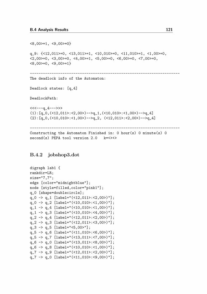
B.4 Analysis Results 121
<8,00>=1, <9,00>=0}
q_9: {<12,011>=0, <13,011>=1, <10,010>=0, <11,010>=1, <1,00>=0,<2,00>=0, <3,00>=0, <4,00>=1, <5,00>=0, <6,00>=0, <7,00>=0,<8,00>=0, <9,00>=1}
---------------------------------------------------------------------The deadlock info of the Automaton:
Deadlock states: [q_4]
DeadlockPath:
<<<---q_4--->>>(1):[q_0,(<12,011>:<2,00>)-->q_1,(<10,010>:<1,00>)-->q_4](2):[q_0,(<10,010>:<1,00>)-->q_2, (<12,011>:<2,00>)-->q_4]
---------------------------------------------------------------------Constructing the Automaton Finished in: 0 hour(s) 0 minute(s) 0second(s) PEPA tool version 2.0 k=<><>
B.4.2 jobshop3.dot
digraph lab1 {rankdir=LR;size="7,7";edge [color="midnightblue"];node [style=filled,color="pink1"];q_0 [shape=doublecircle];q_0 -> q_1 [label="(<12,011>:<2,00>)"];q_0 -> q_2 [label="(<10,010>:<1,00>)"];q_1 -> q_4 [label="(<10,010>:<1,00>)"];q_1 -> q_3 [label="(<10,010>:<4,00>)"];q_2 -> q_4 [label="(<12,011>:<2,00>)"];q_2 -> q_3 [label="(<12,011>:<3,00>)"];q_3 -> q_5 [label="<5,00>"];q_5 -> q_6 [label="(<11,010>:<6,00>)"];q_5 -> q_7 [label="(<13,011>:<7,00>)"];q_6 -> q_0 [label="(<13,011>:<8,00>)"];q_6 -> q_8 [label="(<10,010>:<1,00>)"];q_7 -> q_9 [label="(<12,011>:<2,00>)"];q_7 -> q_0 [label="(<11,010>:<9,00>)"];

122 Design and Demonstration of the Tool
q_8 -> q_2 [label="(<13,011>:<8,00>)"];q_9 -> q_1 [label="(<11,010>:<9,00>)"];}
B.4.3 jobshop3.ps
q_0
q_1
(<12,011>:<2,00>)
q_2
(<10,010>:<1,00>)
q_4(<10,010>:<1,00>)
q_3
(<10,010>:<4,00>)
(<12,011>:<2,00>)(<12,011>:<3,00>)
q_5<5,00> q_6(<11,010>:<6,00>)
q_7
(<13,011>:<7,00>)(<13,011>:<8,00>)
q_8(<10,010>:<1,00>)
(<11,010>:<9,00>)
q_9
(<12,011>:<2,00>)
(<13,011>:<8,00>)
(<11,010>:<9,00>)
Figure B.2: Automaton of jobshop3
B.5 Source Code
Please refer to the CD attached with this thesis.
Bibliography
[1] http://www.graphviz.org/About.php.
[2] http://www.antlr.org/.
[3] http://www.Junit.org/.
[4] The dot language. http://www.graphviz.org/doc/info/lang.html.
[5] Drawing graphs with dot. 2002.
[6] The Not So Short Introduction to Latex2e. 2005.
[7] J. C. M. Baeten. A brief history of process algebra. Theor. Comput. Sci.,335(2-3):131–146, 2005.
[8] J. C. M. Baeten, J. A. Bergstra, and S. A. Smolka. Axiomatizing probabilis-tic processes: Acp with generative probabilities. Inf. Comput., 121(2):234–255, 1995.
[9] Jan A. Bergstra and Jan Willem Klop. Acttau: A universal axiom systemfor process specification. In Algebraic Methods: Theory, Tools and Appli-cations [papers from a workshop in Passau, Germany, June 9-11, 1987],pages 447–463, London, UK, 1989. Springer-Verlag.
[10] Bodei, Degano, Nielson, and Nielson. Static analysis for the pi-calculuswith application to security. INFCTRL: Information and Computation(formerly Information and Control), 168, 2001.
[11] C. Bodei, M. Buchholtz, P. Degano, F. Nielson, and H. Nielson. Automaticvalidation of protocol narration, 2003.
124 BIBLIOGRAPHY
[12] Chiara Braghin, Agostino Cortesi, Riccardo Focardi, Flaminia L. Luccio,and Carla Piazza. Complexity of nesting analysis in mobile ambients.
[13] P. Cousot and R. Cousot. Systematic design of program analysis frame-works. In Conference Record of the Sixth Annual ACM SIGPLAN-SIGACTSymposium on Principles of Programming Languages, pages 269–282, SanAntonio, Texas, 1979. ACM Press, New York, NY.
[14] E. W. Dijkstra. A note on two problems in connexion with graphs. Nu-merische Mathematik, 1(1):269–271, December 1959.
[15] Hanne Riis Nielson Flemming Nielson. Data flow analysis for ccs. 2006.
[16] Hanne Riis Nielson Flemming Nielson. A monotone framework for ccs.2006.
[17] Emden Gansner, Eleftherios Koutsofios, and Stephen North. Drawinggraphs with dot, 2006.
[18] Stephen Gilmore. The pepa workbench: User’s manual. 2001.
[19] Stephen Gilmore and Jane Hillston. The PEPA workbench: A tool tosupport a process algebra-based approach to performance modelling, 1994.
[20] G.Lowe. Probabilities and priorities in timed csp. 1999.
[21] Flemming Nielson Hanne Riis Nielson. Semantics with Applications – AFormal Introduction. Wiley Professional Computing, 1992.
[22] J. Hillston. A compositional approach to performance modelling. Cam-bridge University Press, 1996.
[23] J. Hillston. Process algebras for quantitative analysis. In LICS ’05: Pro-ceedings of the 20th Annual IEEE Symposium on Logic in Computer Sci-ence (LICS’ 05), pages 239–248, Washington, DC, USA, 2005. IEEE Com-puter Society.
[24] C. A. R. Hoare. Communicating sequential processes. Commun. ACM,21(8):666–677, 1978.
[25] John E. Hopcroft and Jeffrey D. Ullman. Introduction To Automata Theory,Languages, And Computation. Addison-Wesley Longman Publishing Co.,Inc., Boston, MA, USA, 1990.
[26] R. Milner. A Calculus of Communicating Systems. Springer-Verlag NewYork, Inc., Secaucus, NJ, USA, 1982.
[27] M. Neubauer and P. Thiemann. An implementation of session types, 2004.

BIBLIOGRAPHY 125
[28] Flemming Nielson, Hanne R. Nielson, and Chris Hankin. Principles ofProgram Analysis. Springer-Verlag New York, Inc., Secaucus, NJ, USA,1999. Second printing, 2005.
[29] Hanne Riis Nielson and Flemming Nielson. Shape analysis for mobile am-bients. In POPL ’00: Proceedings of the 27th ACM SIGPLAN-SIGACTsymposium on Principles of programming languages, pages 142–154, NewYork, NY, USA, 2000. ACM Press.
[30] N.V.Haenel. User guide for the java edition of the pepa workbench. Tabascorelease, version 0.9.4, 2004.
[31] R.Milner. Communication and Mobile Systems: The pi-Calculus. Cam-bridge University Press, 1st edition,1999.
[32] Andrew S. Tanenbaum. Modern Operating Systems, 2nd Edition. PrenticeHall., 2001.
[33] Antti Valmari. The state explosion problem. In Lectures on Petri Nets I:Basic Models, Advances in Petri Nets, the volumes are based on the Ad-vanced Course on Petri Nets, pages 429–528, London, UK, 1998. Springer-Verlag.
[34] V. Vasconcelos, A. Ravara, and S. Gay. Session types for functional multi-threading, 2004.
[35] Wikipedia. Process calculus. http://en.wikipedia.org/wiki/Processcalculi.


![Solving Infinite Stochastic Process Algebra Models Through ...qav.comlab.ox.ac.uk/papers/papm99.pdf · 3 Matrix-Geometric Methods 3.1 Introduction The Matrix-Geometric Method [16,3,4]](https://static.fdocuments.in/doc/165x107/5f3f598df7b31a6ba2369a10/solving-ininite-stochastic-process-algebra-models-through-qav-3-matrix-geometric.jpg)