Statistical Models Applied to the Rating of Sports Teams

Honors Project: Mathematics

by Kenneth Massey

Spring 1997

Bluefield College

Sponsoring Professor: Mr. Alden Starnes

Sponsoring English Professor: Dr. Wayne Massey

Table of Contents

1: Sports Rating Models 1

2: Linear Regression 6

3: Solving Systems of Linear Equations 20

4: Least Squares Ratings 31

5: Maximum Likelihood Ratings 49

6: The Elecs Rating Method 67

Appendix: An Application to College Football 77

Bibliography 80

1

Chapter 1: Sports Rating Models

Introduction

One of the most intriguing aspects of sports is that it thrives on controversy. Fans, the media,

and even players continually argue the issue of which team is best, a question that can ultimately be

resolved only by playing the game. Or can it? It is likely that a significant portion of sporting results

could be regarded as flukes. Simply put, the superior team does not always win. Therefore even a

playoff, although it may determine a champion, will not necessarily end all disagreement as to which

team is actually the best.

Given the broad subjectivity of sports in general, it is of great popular interest to develop

some standard by which all teams can be evaluated. Traditionally, win-loss standings have served

this purpose. Unfortunately, there are several obvious weaknesses inherent in this measure of a

team’s strength. Among them is the assumption that each team plays a similar schedule. This

requirement is not met in leagues with a large number of teams, such as most college athletics. The

alternative usually adopted is a poll, which is conducted by certain media experts or others associated

with the sport. Despite what may be good intentions, voter bias is inevitable either because of

history, differences in publicity, or personal opinion.

These difficulties suggest the implementation of mathematically based methods of measuring

a team’s ability. Since a variety of models is available for consideration, subjectivity is not entirely

eliminated. However, it exists only in the choice and development of the model, and can be

completely identified in advance. Furthermore, once an appropriate model has been selected, the

results will always be purely objective and consistent within the framework of that particular system.

2

At this point, it is appropriate to discuss some terminology. First we make the distinction

between a rating and a ranking. A ranking refers only to the ordering of the teams (first, second,

third, ...). However, a rating comes from a continuous scale such that the relative strength of a team

is directly reflected in the value of its rating (Stern 1995). Hence it is possible to determine the

actual separation in ability for teams that may be adjacent in the rankings. A rating system assigns

each team a single numerical value to represent that team’s strength relative to the rest of the league

on some predetermined scale. In particular, we are interested in mathematical rating systems, which

have the additional requirement that the ratings be interdependent. Consequently, they must be

recalculated, typically with the aid of a computer, from scratch whenever new results are obtained

from actual games. This is in contrast to accumulation rating systems, such as the point system in

professional hockey, in which ratings are merely updated from their previous values.

Although rating models can be tailored to incorporate the distinctive features of various

sports, this paper focuses only on more general methods. Therefore, it is desirable that we limit the

amount of data that are required to compute a set of ratings. Often the only information available

is the final score, perhaps including which team was at home. This much is common to virtually all

sports, and is usually a sufficient indicator of how the game was played.

In the course of developing a rating system, it is necessary to determine exactly what the

ratings are intended to accomplish. Should ratings reward teams that deserve credit for their

consistent season long performance, or should they determine which teams are actually stronger in

the sense that they would be more likely to win some future matchup? The first objective is usually

emphasized if the ratings are meant to determine a champion or those teams that should qualify for

the playoffs. In this case, results should attempt to explain past performances. Popular interest in

3

these ratings peaks when there is intense disagreement that cannot be resolved on the field. This is

quite common in college football, in which there is no playoff to decide the national championship.

For example, in 1994 Nebraska and Penn State both finished the season undefeated. The AP and

Coaches’ polls both awarded the championship to Nebraska. However, widely respected rating

systems published by the USA Today and the New York Times both concluded that Penn State was

more deserving.

Other rating systems are designed to be a tool for predicting future game outcomes. These

models are often characterized by the use of past seasons’ data and features that account for the long

and short term variability of a team’s performance. The success of these more complex methods is

quite remarkable. Glickman and Stern have documented convincing evidence that statistical models

are more accurate than the Las Vegas point spread, despite the lack of information pertaining to

intangible factors such as motivation. In fact, they report a 59% (65 out of 110) success rate in

predicting NFL football games against the spread (Glickman 1996). Unfortunately the gambling

establishment has made extensive use of similar statistical models. To a certain degree, the ability

to make predictions is inherent in any rating model because of its association with inferential

statistics. The intent, however, of the rating systems presented in this paper is not to promote this

aspect of predicting future outcomes for the purposes of gambling.

History

The history of sports rating systems is surprisingly long. As early as the 1930's, the

Williamson college football system was widely published. The Dunkel Index is another classic,

dating back to 1955 (Stefani 1980). In more recent memory, the USA Today has printed the results

4

of Jeff Sagarin’s ratings for most major American sports. Other newspapers frequently list computer

ratings for local high school teams. Even the NCAA has acknowledged the benefits of rating

systems by adopting the Rating Percentage Index (RPI) to help decide the field for their annual

basketball tournament. Besides its widespread infiltration of the popular media, rating methodology

has also been discussed in formal literature such as statistical journals.

Despite the long history, there is no comparison to the tremendous explosion of rating

systems that has occurred in the last two years. This can be attributed primarily to the expanding

popularity of the internet. Amateur and professional statisticians from around the country now have

a platform on which to tout their concept of the ideal model for rating sports teams. No fewer than

thirty six different systems are now published on the World Wide Web. A complete listing for

college football is available at http://www.cae.wisc.edu/~dwilson/rsfc/rate/index.html.

Applications

For most people, the results of rating systems are interesting primarily as a form of

entertainment. They contribute to the controversies in sports as much as they help settle them. This

proves an interesting fact: the mathematical sciences are not limited to theory and its meaningful

application. Ratings are completely trivial except as yet another aspect of sports, whose purpose is

not rooted in anything other than fun and relaxation.

This does not imply that rating models themselves cannot be applied to other practical

situations. In particular, the mathematical background necessary to develop certain rating systems

has been adapted to fields as diverse as economics and artificial intelligence. Another potentially

significant use of rating models is in the classroom. Dr. David Harville, a professor of statistics at

5

Iowa State University states: “As a teacher and student, we have found the application of linear

models to basketball scores to be very instructive and recommend the use of this application in

graduate level courses in linear models. College basketball gives rise to several questions that can

be addressed by linear statistical inference and that may generate interest among the students.” He

goes on to describe how certain features of sports ratings are helpful in illustrating various theoretical

concepts, giving insight as to why they work (Harville 1994).

The remainder of this paper deals with both the foundational theory and the practical

application of sports ratings. Essentially two models are discussed, each representative of a class

of popular rating systems. In each case, the model is developed mathematically, and possible

implementation algorithms are discussed. When appropriate, I have attempted to provide some

simple examples to illustrate the ideas being presented. These examples are contrived; however the

appendix contains several results from rating models that have been applied to actual situations in

the real world.

6

Chapter 2: Linear Regression

Many rating models utilize techniques of linear regression. In particular, the least squares

rating methods discussed in chapter four rely heavily on the background information presented in

this chapter. A general understanding of these statistical procedures allows us to adapt them to serve

our specific purposes, while providing insight into possible application in many other diverse

situations. This chapter is devoted to the mathematical derivation of regression. Special emphasis

is placed on the conditions necessary to calculate a linear regression and various interpretations that

can be applied to the results.

The purpose of a regression is to express the mean value of a dependent response variable,

Y, as a function of one or more independent predictor variables, x1,x2,...,xk. This function will be

considered to have a linear form. Although the predictors are not treated as random variables, the

conditional response Y*x1,x2,...,xk is assumed to be a random variable. Referring to the predictors

as x in vector notation, the general linear model takes the form:

µY | x = $1f1(x) + $2f2(x) + ... + $nfn(x)

or

Y = $1f1(x) + $2f2(x) + ... + $nfn(x) + E

where E is a random variable with mean zero (Arnold 1995). A particular instance of Y is denoted

by:

y = $1f1(x) + $2f2(x) + ... + $nfn(x) + ,

The error term , is a realization of E. It corresponds to the difference between the observed value

y and the true regression line.

7

The functions f1,f2,...,fn, are chosen by the experimenter, and their values can be computed

directly since the independent variables, x, are known either through intentional design or by random

observation along with the dependent variable y. However the model parameters, $ = $1,$2,...,$n are

unknown and must be estimated by b = b1,b2,...,bn. It is generally impossible to find a curve of

regression that matches each piece of observational datum exactly. Therefore, for any particular

observation i with predictors x(i), unexplained error called the residual exists as

ei = yi - [ b1f1(x(i)) + b2f2(x

(i)) + ... + bnfn(x(i)) ] = yi - íi

The residual corresponds to the difference between the observed response y and the estimated

response í. Because the parameters b are only estimates of $, the error term is expressed by ei

instead of ,i.

Statistical estimates for b are obtained by the least squares method, which minimizes the total

squared error, 3ei2. Squaring the error terms serves two purposes. First since e2$ 0, the error terms

can never be negative, thereby cancelling each other out. Second it causes many small variations to

be prefered over a few dramatic inconsistencies. In essence, coefficients are chosen so that the

curve of regression comes as close as possible to all data points simultaneously (Arnold 1995).

A set of m observations forms a system of m equations in n unknowns:

y1 = b1f1(x(1)) + b2f2(x

(1)) + ... + bnfn(x(1)) + e1

y2 = b1f1(x(2)) + b2f2(x

(2)) + ... + bnfn(x(2)) + e2

:::::::::::::::::::::::::::::::::::::::::::::::::::::::::::::::::

ym = b1f1(x(m)) + b2f2(x

(m)) + ... + bnfn(x(m)) + em

To simplify our work, this system can be expressed in matrix-vector form as

y = Xb + e = í + e

where xij = fj(x(i)). Do not confuse the set of dependent variables x(i) with the model specification

8

matrix X.

As mentioned before our task is to choose model parameters, or coeffiecients, that minimize

the sum of all the squared error terms.

f(b) = e12 + e2

2 + ... + em2 = 3 i=1..m ei

2 = eTe = (y - Xb)T (y - Xb)

One approach to minimizing the preceding function is to take partial derivatives with respect to each

bi and set them equal to zero. Algebraicly this is quite an involved process. However there are

several rules of matrix differentiation that will simplify the task. Not surprisingly, because matrix

operations are merely extentions of real number arithmetic, these rules are analogous to the familiar

methods used in standard calculus.

Definition 2.1

Let x be a n dimensional vector and y = f(x) be a m dimensional vector. Then is defined

as the (m x n) matrix Z. Where

Theorem 2.1

If x, y = f(x), and z = g(x) are vectors, A is a matrix, and c is a real number then

i. if y is a constant

ii.

9

iii.

iv.

v.

vi.

vii. where y = f(u) and u = g(x)

It is assumed that the derivatives exist and that matrix multiplications are compatible. The proof

follows directly from definition 1.1 and standard results from calculus (Myers 1992). #

Returning to our original equation we wish to minimize the function,

f (b) = (y - Xb)T (y - Xb)

Taking the first derivative with respect to b we have

rules iv. and vii.

rules i., ii., and iii.

rule v.

Setting f N(b) equal to zero and using rules of matrix manipulation,

0T = -2 (y - Xb)T X

= (y - Xb)T X

0 = [(y - Xb)T X]T

10

Figure 1

= XT(y - Xb)

= XTy - XTXb

XTXb = XTy

These are called the normal equations of the regression; they correspond to a critical point

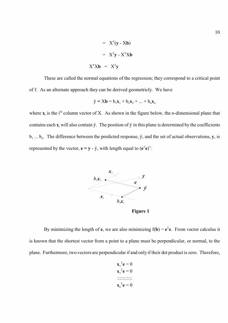
of f. As an alternate approach they can be derived geometricly. We have

í = Xb = b1x1 + b2x2 + ... + bnxn

where xi is the ith column vector of X. As shown in the figure below, the n-dimensional plane that

contains each xi will also contain í. The position of í in this plane is determined by the coefficients

b1 ... bn. The difference between the predicted response, í, and the set of actual observations, y, is

represented by the vector, e = y - í, with length equal to (eTe)½.

By minimizing the length of e, we are also minimizing f(b) = eTe. From vector calculus it

is known that the shortest vector from a point to a plane must be perpendicular, or normal, to the

plane. Furthermore, two vectors are perpendicular if and only if their dot product is zero. Therefore,

x1Te = 0

x1Te = 0

:::::::::::

xnTe = 0

11

Combining these equations we see that,

XTe = XT(y - Xb) = 0

XTXb = XTy

which is equivalent to our previous result.

To verify that a solution to these normal equations does minimize f(b) we differentiate again

This result is equivalent to the Hessian matrix of the multivariable function f. Letting Hf = 2XTX,

we see that by definition, hij = . Furthermore, Hf is positive definite since the quadratic form

is positive for any vector v � 0.

vTHfv = vT(2XTX)v = 2(Xv)T(Xv) > 0

It can be shown that a matrix is positive definite if and only if each of its eigenvalues is positive

(Rabenstein 1992). Also, a multivariable function, f, has a strict local minimum at a critical point

if each eigenvalue of the Hessian matrix Hf is positive at that point (Trotter 1996). Therefore, f(b)

is minimized whenever b is a solution to the normal equations.

To solve the normal equations for b we notice that the matrix equation,

12

XTXb = XTy

corresponds to a system of m equations in m unknowns. If XTX has an inverse we can multiply both

sides of the equation by (XTX)-1 yielding

b = (XTX)-1XTy

However, in general this inverse will not always exist. What conditions are sufficient to guarantee

that a unique solution can be found? We will first need the following results.

Definition 2.2

The row rank of a m x n matrix A is the dimension of the subspace of Rn spanned by the row

vectors of A. Similarly, the column rank is the dimension of the subspace of Rm spanned by the

column vectors. The rank of A can be shown to equal the common value of the row and column

ranks (Rabenstein 1992). Rank can be defined equivalently as the size of the largest set of linearly

independent row / column vectors of A (Cormen 1992).

Definition 2.3

A null vector for a matrix A is any vector v � 0 such that Av = 0 (Cormen 1992).

It follows from these definitions that if a matrix has no null vectors then the column vectors must

be independent and the matrix has full column rank. If a null vector does exist then at least one

column vector can be expressed as a linear combination of the others, and therefore the column

vectors are dependent.

13

Theorem 2.2

If A is a matrix and v is a vector, then v will be a null vector of ATA if and only if v is a null

vector of A.

Proof

First suppose that v is a null vector of A. Then Av = 0 and

(ATA)v = AT(Av) = AT0 = 0

Therefore v is also a null vector of ATA.

Now suppose that v is a null vector of ATA. Then (ATA)v = 0, and we can create the

quadratic form by multiplying each side of the equation by vT.

vT(ATA)v = vT0 = 0

0 = vT(ATA)v = (Av)T(Av) = 2Av22

The norm of any vector is zero if and only if that vector is 0. Therefore Av = 0 and v must be a null

vector of A. #

Theorem 2.3

If Ab = y corresponds to a m x m system of linear equations then a solution will exist if and

only if every null vector of AT is also a null vector of yT. The solution will be unique if and only if

A has no null vectors.

Proof

Assume a solution b exists. We know that if v is a null vector of AT then

Ab = y

14

(Ab)T = yT

bTAT = yT

bTATv = yTv

0 = yTv

Hence, each null vector of AT is also a null vector of yT.

The system described by Ab = y can be reduced to row-echelon form, ANb = yN. If any row,

ak, of A is eliminated then the required elementary row operations are represented by 3i=1..m viai =

0, where ai denotes the ith row of A. The appropriate constants, v1...vm, constitute a null vector, so

akN = ATv = 0. If we assume that every null vector of AT is also a null vector of yT, then we have ykN

= yTv = 0. The kth equation becomes 0b = akNb = ykN = 0, which is always true. Therefore if the

system is in row-echelon form, then for any k such that akN= 0, bk can be chosen arbitrarily. The

remaining elements of b will then be expressed in terms of these arbitrary elements. Consequently

a solution exists.

If A has no null vectors, then the column vectors are independent and det(A) � 0. Therefore

the system possesses a unique solution (Rabenstein 1992).

Whenever a unique solution exists, A must be nonsingular with no null vectors. Otherwise,

at least one row of the row-echelon matrix would be 0 and the corresponding bk could be chosen

arbitrarily. #

Theorem 2.4

The normal equations, XTXb = XTy, of a linear regression always have a solution. This

15

solution is unique if and only if X has full column rank, or equivalently, X has no null vector.

Proof

The normal equations correspond to a m x m system of equations. If v is a null vector of

(XTX)T = XTX. Then by Theorem 2.2, v is also a null vector of X. Therefore

(XTy)Tv = (yTX)v = yT(Xv) = yT0 = 0

Theorem 2.3 implies that the system has a solution.

Assume that X has no null vector. We know by Theorem 2.2 that this is also true for XTX.

Therefore by Theorem 2.3 there exists a unique solution. Furthermore, det(XTX) � 0 so XTX is

invertible (Rabenstein 1992). Solving the normal equations for b yields

b = (XTX)-1XTy

Now assume a unique solution exists. By Theorem 2.3, we know that XTX cannot have a null

vector. Therefore by Theorem 2.2, X must also have full column rank and no null vector. #

We have shown that if X has full column rank in a linear regression then a unique vector of

parameters, b, can be found to minimize the squared error for the set of observations.

b = [(XTX)-1XT]y = X+y

The term pseudoinverse refers to X+, and is a natural generalization of X-1 to the case in which X is

not square (Cormen 1992). Instead of providing an exact solution to Xb = y, multiplying by the

pseudoinverse gives the solution that provides the best “fit” for an overdetermined system of

equations. If X is square then

X+X = [(XTX)-1XT]X = I

so the pseudoinverse is identical to the traditional inverse, X-1.

16

An interesting interpretation of least squares estimators is that each bk, k=1..n, is simply a

weighted average. To see this consider the normal equations XTXb = XTy. The elements of XTX

and XTy can be expressed this way:

(XTX)ij = xi@xj

(XTy)i = xi@y

where xi is the ith column vector of X.

Now take the row corresponding to any one of the normal equations. Using the kth row we

have

b1xk@x1 + b2xk@x2 + ... + bnxkxn = xk@y

bkxk@xk = xk@y - 3j�k bjxk@xj

bkxk@xk = xk@(y - 3j�k bjxj)

In scalar notation this becomes

17

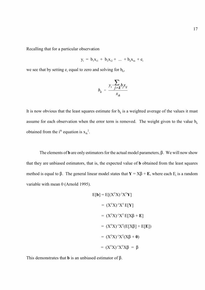
Recalling that for a particular observation

yi = b1xi1 + b2xi2 + ... + bnxin + ei

we see that by setting ei equal to zero and solving for bk,

It is now obvious that the least squares estimate for bk is a weighted average of the values it must

assume for each observation when the error term is removed. The weight given to the value bk

obtained from the ith equation is xik2.

The elements of b are only estimators for the actual model parameters, $. We will now show

that they are unbiased estimators, that is, the expected value of b obtained from the least squares

method is equal to $. The general linear model states that Y = X$ + E, where each Ei is a random

variable with mean 0 (Arnold 1995).

E[b] = E[(XTX)-1XTY]

= (XTX)-1XT E[Y]

= (XTX)-1XT E[X$ + E]

= (XTX)-1XT(E[X$] + E[E])

= (XTX)-1XT(X$ + 0)

= (XTX)-1XTX$ = $

This demonstrates that b is an unbiased estimator of $.

18

Least squares estimators are not the only unbiased estimators of $ that can be found for a

particular regression. In fact, b = (ATX)-1ATy is unbiased for any (m x n) matrix A.

E[b] = E[(ATX)-1ATY]

= (ATX)-1AT E(Y)

= (ATX)-1AT(X$) = $

The least squares results are then equivalent to the specific case where A = X.

A set of unbiased estimators can be derived by minimizing the function:

f(b) = (AT(y - Xb))T(AT(y - Xb))

Taking the derivative with respect to b and setting it equal to zero shows us that

fN(b) = -2(AT(y - Xb))T(ATX)

0 = (AT(y - Xb))T(ATX)

= (XTA)AT(y - Xb)

(XTA)-10 = 0 = AT(y - Xb)

ATXb = ATy

b = (ATX)-1ATy

Notice that ATX must be invertible. This vector b minimizes f since the second derivative with

respect to b is equal to (ATX)T(ATX), which is a positive definite Hessian matrix.

If we interpret b as a set of weighted averages then it can be shown that for all k=1..n

19

The elements of A can be chosen arbitrarily to control the significance that should be attributed to

the results of each observation. Instead of weights being equal to xik2, they become aikxik, which

should usually be arranged to be nonnegative.

One final note is that least squares estimators are usually superior to other unbiased linear

estimators in which A � X. Reasons for this include the fact that least squares parameters display

the smallest variance from sample to sample (Degroot 1989). In addition, if certain assumptions are

made about the model distributions, then the least squares estimators are equivalent to the maximum

likelihood estimators of the regression.

20

Chapter 3: Solving Systems of Linear Equations

Many rating performance models, especially those involving least squares regression, require

solving systems of simultaneous linear equations. Although software packages that provide

“MatrixSolve” procedures are readily available, it is of sufficient interest to understand how linear

systems are solved so that necessary adjustments can be made for a particular problem, either to

maximize efficiency or provide a specific feature unique to the situation. A system of linear equations

can be expressed as Ax = b, where A is an order n square matrix and x, b are n-dimensional column

vectors. For simplicity, we will assume that a unique solution exists, so A must be nonsingular.

General methods of solution can be either direct or iterative. In the former, a fixed number

of operations is necessary to obtain the solution. Consequently, an upper bound for the time required

is known in advance. However, direct methods have the disadvantage of being prone to round off

error that accumulates with repeated floating point operations on real numbers, which must be

represented by computers with a maximum number of significant digits. Error terms tend to be

magnified with each calculation since direct methods have no self-correcting qualities. In contrast,

iterative methods are virtually free of round off error since they operate in a loop that exhibits self-

correcting behavior and never alters the composition of the original matrix. Iterative methods also

have the benefit of initial approximations that may lead to fast convergence, and the process may be

halted at any predetermined tolerance level. However, there is no guarantee of speedy convergence.

In fact, iterative procedures may not converge at all.

To provide flexibility and an opportunity for comparison, let us look at an example of both

methods. In each case an algorithm was chosen that represents a typical tradeoff of power versus

21

generality. First, consider the direct method known as LUP decomposition (Cormen 1992).

LUP Decomposition

LUP decomposition is based on Gaussian elimination, a familiar method for solving systems

of linear equations. First the coefficient part of the augmented matrix representing the system is

converted to upper triangular form by applying elementary row operations. Then backward

substitution is used to solve for the unknown variables.

Although the basic Gaussian elimination algorithm is efficient and relatively stable, there is

a significant drawback when it must be implemented on the same coefficient matrix with different

right-side vectors. For example, consider the two equations, Ax = b and Ax = d. A careful

examination of the standard Gaussian process reveals that the same row operations are applied to

each set of equations. This is a direct consequence of the fact that the coefficient matrices are

identical, and both must be made upper triangular. In a sense the right-side vectors, b and d, are

merely along for the ride. They are not necessary in defining the elimination process; only in the

backward substitution do they become important.

It is wasteful to repeat the manipulation of the coefficient matrix when only the right-side

vector has changed. However in order to solve a particular system, the row operations must be

applied to the entire augmented matrix, which includes the right-side vector. This dilemma suggests

a slight alteration of the general Gaussian method, allowing it to “remember” the row operations

previously used.

LUP decomposition factors A into three (n x n) matrices L, U, and P, such that PA = LU.

The matrix L is unit lower triangular, U is upper triangular, and P is a permutation matrix that has

22

the effect of rearranging the rows of A. We have LUx = PAx = Pb. After the decomposition has

been found, the solution x can be computed for any b. First let y = Ux and solve Ly = Pb for y. This

is easily accomplished with forward substitution since L is lower triangular. Then, in a similar use

of backward substitution on the upper triangular matrix U, solve Ux = y for x.

It turns out that U is exactly the same matrix found in basic Gaussian elimination, and L and

P store the necessary row additions and exchanges respectively. In solving Ly = Pb, we are

essentially duplicating the series of row operations previously applied to A to form U.

To understand the derivation of a LUP decomposition, consider the Gaussian elimination

algorithm as applied to the coefficient matrix A. A nonzero element is placed in the upper left

position by swapping rows if necessary. This strategy, called pivoting, is equivalent to multiplying

A by a permutation matrix P1. Setting Q = P1A, we partition Q into four parts:

where w is a n-1 dimensional row vector, v is a n-1 dimensional column vector, and QN is an order

n-1 square submatrix of Q. The permutation matrix P1 is chosen to guarantee that q11 is nonzero.

Eliminating the elements represented by v is accomplished by subtracting appropriate

multiples of the first row. If we represent this as a matrix multiplication, then

23

Assuming that A was nonsingular, QN-vw/q11 must also be nonsingular. Otherwise

det(Q) = 0, so det(A) = 0 and we have a contradiction. Therefore the decomposition process can

be applied recursively to QN-vw/q11 (Cormen 1992). This yields a LUP decomposition for QN-vw/q11

that can be expressed as LNUN = P2'(QN-vw/q11). We rearrange the rows again by setting

This last operation is a LU multiplication, since the first matrix is lower triangular and the second

is upper triangular. Combining our results we see that

P2Q = P2(P1A) = PA = LU

where the final permutation matrix P = P2P1.

24

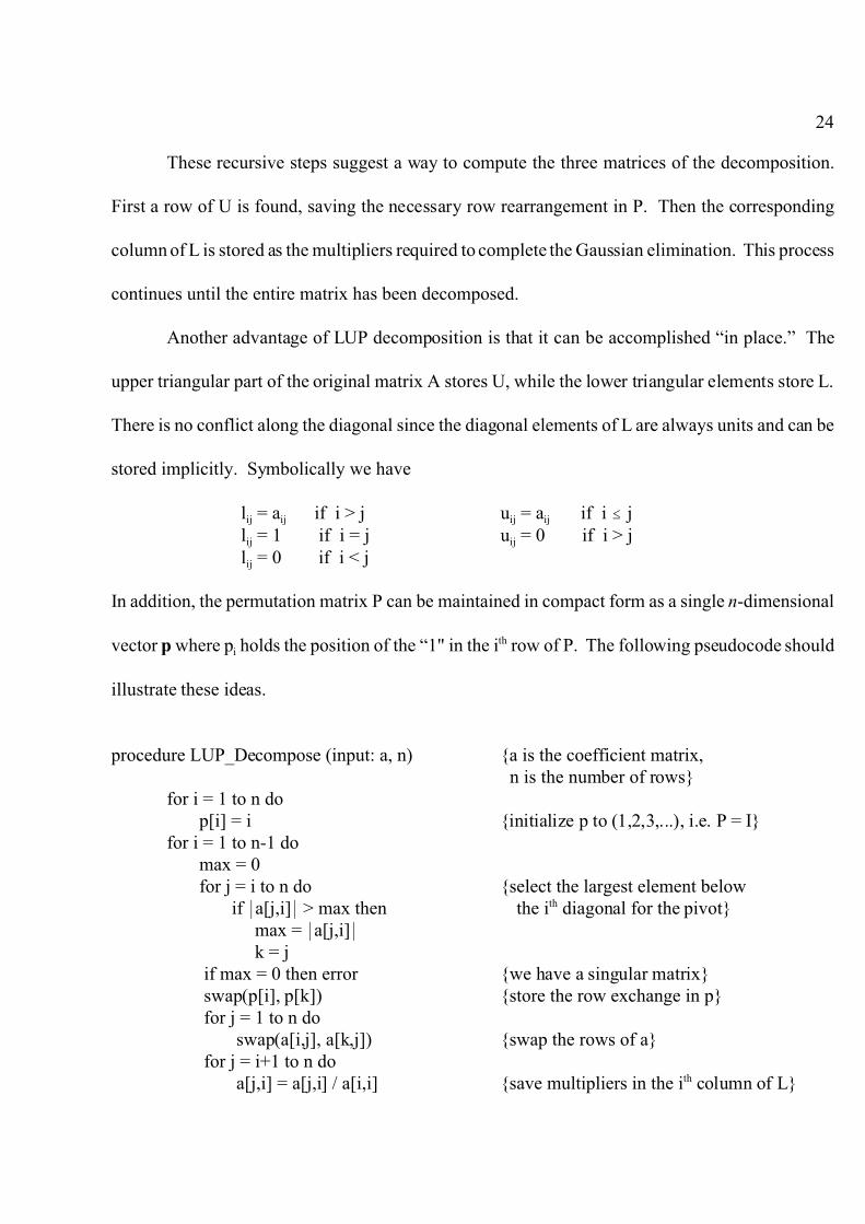
These recursive steps suggest a way to compute the three matrices of the decomposition.

First a row of U is found, saving the necessary row rearrangement in P. Then the corresponding

column of L is stored as the multipliers required to complete the Gaussian elimination. This process

continues until the entire matrix has been decomposed.

Another advantage of LUP decomposition is that it can be accomplished “in place.” The

upper triangular part of the original matrix A stores U, while the lower triangular elements store L.

There is no conflict along the diagonal since the diagonal elements of L are always units and can be

stored implicitly. Symbolically we have

lij = aij if i > j uij = aij if i # j lij = 1 if i = j uij = 0 if i > j lij = 0 if i < j

In addition, the permutation matrix P can be maintained in compact form as a single n-dimensional

vector p where pi holds the position of the “1" in the ith row of P. The following pseudocode should

illustrate these ideas.

procedure LUP_Decompose (input: a, n) {a is the coefficient matrix, n is the number of rows}

for i = 1 to n do p[i] = i {initialize p to (1,2,3,...), i.e. P = I}for i = 1 to n-1 do max = 0 for j = i to n do {select the largest element below if *a[j,i]* > max then the ith diagonal for the pivot}

max = *a[j,i]* k = j

if max = 0 then error {we have a singular matrix} swap(p[i], p[k]) {store the row exchange in p} for j = 1 to n do

swap(a[i,j], a[k,j]) {swap the rows of a} for j = i+1 to n do

a[j,i] = a[j,i] / a[i,i] {save multipliers in the ith column of L}

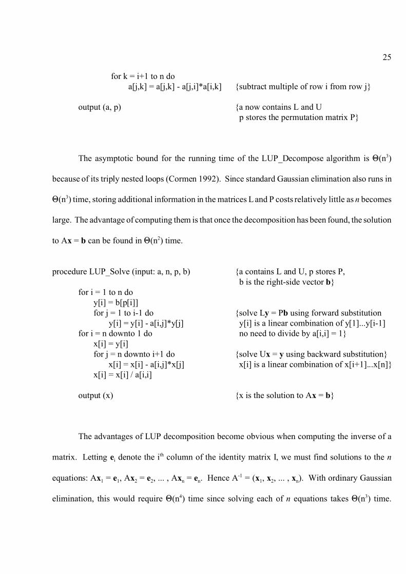
25

for k = i+1 to n do a[j,k] = a[j,k] - a[j,i]*a[i,k] {subtract multiple of row i from row j}

output (a, p) {a now contains L and U p stores the permutation matrix P}

The asymptotic bound for the running time of the LUP_Decompose algorithm is 1(n3)

because of its triply nested loops (Cormen 1992). Since standard Gaussian elimination also runs in

1(n3) time, storing additional information in the matrices L and P costs relatively little as n becomes

large. The advantage of computing them is that once the decomposition has been found, the solution

to Ax = b can be found in 1(n2) time.

procedure LUP_Solve (input: a, n, p, b) {a contains L and U, p stores P, b is the right-side vector b}

for i = 1 to n do y[i] = b[p[i]] for j = 1 to i-1 do {solve Ly = Pb using forward substitution

y[i] = y[i] - a[i,j]*y[j] y[i] is a linear combination of y[1]...y[i-1]for i = n downto 1 do no need to divide by a[i,i] = 1} x[i] = y[i] for j = n downto i+1 do {solve Ux = y using backward substitution}

x[i] = x[i] - a[i,j]*x[j] x[i] is a linear combination of x[i+1]...x[n]} x[i] = x[i] / a[i,i]

output (x) {x is the solution to Ax = b}

The advantages of LUP decomposition become obvious when computing the inverse of a

matrix. Letting ei denote the ith column of the identity matrix I, we must find solutions to the n

equations: Ax1 = e1, Ax2 = e2, ... , Axn = en. Hence A-1 = (x1, x2, ... , xn). With ordinary Gaussian

elimination, this would require 1(n4) time since solving each of n equations takes 1(n3) time.

26

However with LUP decomposition, calculating the inverse can be done within the 1(n3) bound. An

initial call to LUP_Decompose runs in 1(n3) time, and n subsequent calls to LUP_Solve take 1(n2)

each for a total of 1(n3) running time. The increase in work required to solve n equations instead

of only one is represented by a constant factor, which does not contribute to asymptotic growth.

In some applications, especially eigenvector problems, we wish to solve left handed

equations of the form xTA = bT. Taking the transpose of each side we see that ATx = b. There is an

obvious similarity to the original problem of Ax = b, and in fact it is possible to use the same LUP

decomposition to solve both cases.

If A has been decomposed, then we know that PA = LU. It can be shown that for any

permutation matrix, P-1 = PT (Burden 1993). Therefore we have

P-1PA = P-1LU

A = PTLU

AT = (LU)TP = UTLTP = LNUNP

Notice that LN is lower triangular, while UN is unit upper triangular. After the decomposition of A,

the elements of LN and UN are simply the transposed elements of U and L respectively. The system

ATx = b can now be written as LNUNPx = b. Forward substitution is used to obtain the solution to

LNy = b; then UNPx = y is solved with backward substitution.

procedure LUP_SolveLeft (input: a, n, p, b) {a contains LN = UT and UN = LT, p stores P, b is the right-side vector b}

for i = 1 to n do y[i] = b[i] {solve LNy = b using forward substitution for j = 1 to i-1 do lNij is referenced by uT

ij = uji = a[j,i] y[i] = y[i] - a[j,i]*y[j] y[i] is a linear combination of y[1]...y[i-1]}

y[i] = y[i] / a[i,i] for i = n downto 1 do {solve UNPx = y using backward substitution

27

x[p[i]] = y[i] uNij is referenced by lTij = lji = a[j,i]

for j = n downto i+1 do (Px)i = x[p[i]] is a linear combination of x[p[i]] = x[p[i]] - a[j,i]*x[p[j]] x[p[i+1]]...x[p[n]]}

output (x) {x is the solution to ATx = b}

Iterative Techniques

Iteration provides an alternative to the use of direct methods, such as LUP decomposition,

to solve linear systems. Iterative procedures generate a sequence of approximation vectors,

{x(k)}k=0..4, that converges to the true solution (Burden 1993).

limk64 x(k) = x

We will consider fixed point iteration in which each successive estimate for x is determined from

a function of the form x = f(x) = Tx + c. T is called the iteration matrix and has order n; c is an

n-dimensional column vector. In particular, given x(k-1)

x(k) = f(x(k-1)) = Tx(k-1) + c

The sequence begins with an initial approximation x(0). If the function yields a convergent sequence

of vectors then the limiting value of x(k) will be the unique solution x.

A common example of iteration techniques is the Jacobian method. The system Ax = b can

be written as (D-L-U)x = b, where D is the diagonal matrix and L, U are the negated strictly lower

and upper triangular parts of A. This provides a way to write the vector x as a function of itself.

Dx = (L+U)x + b

x = D-1(L+U)x + D-1b = Tx + c

In the limiting case,

28

x(k) = D-1(L+U)x(k-1) + D-1b

The Jacobian iterative method is based on this formula, which can be expressed in scalar form as

(Stewart 1994). Notice that xi(k) is obtained by simply setting aix

(k-1) = bi and solving for the xi

necessary to satisfy this condition.

In Jacobian iteration, only the components of x(k-1) are used to find the next approximation

vector x(k). However if i>1 then the elements x1(k), x2

(k), ... , xi-1(k) are available when xi

(k)

is calculated. Significant improvement can be achieved by utilizing these more recent values which

are likely to be more accurate than their predecessors x1(k-1), x2

(k-1), ... , xi-1(k-1). This concept is the

basis for Gauss-Seidel iteration.

Returning to the equation Ax = (D-L-U)x = b, as k approaches infinity

(D-L)x(k) = Ux(k-1) + b

x(k) = (D-L)-1Ux(k-1) + (D-L)-1b = Tx(k-1) + c

In practice the vector x(k) is computed one element at a time, each xi(k) replacing the previous estimate

xi(k-1). This can be written as

Dx(k) = Lx(k) +Ux(k-1) + b

x(k) = D-1(Lx(k) +Ux(k-1) + b)

or equivalently,

29

Despite its intimidating mathematical formula, Gauss-Seidel iteration is implemented relatively

easily by the following pseudocode:

procedure Gauss_Seidel (input: a, b, x, n, tol, m) {a is the matrix A, b is the vector b, x contains the initial approximation x(0)

k = 1 n is the size of A, tol is the tolerence level,repeat m is the maximum number of iterations} e = 0 for i = 1 to n do t = b[i] {set t = xi

(k) equal to for j = 1 to n do (-3j=1..i-1 aijxj

(k) - 3j=i+1..n aijxj(k-1) + bi ) / aii }

if i�j then t = t - a[i,j] * x[j] t = t / a[i,i] if *t-x[i]* > e then e = *t-x[i]* {update the vector norm 2x(k) - x(k-1)2 x[i] = t replace x[i] = xi

(k-1) with t = xi(k)}

k = k + 1until (e < tol) or (k > m)

if e > tol then error {not sufficient convergence in m iterations}

output (x) {x is the estimated solution to Ax = b}

The stopping conditions for any iteration technique are somewhat arbitrary. Remembering

that convergence is not guaranteed, the maximum number of iterations should be limited. Small

changes in successive approximations indicate convergence. Therefore any vector norm 2x(k) - x(k-1)2

that measures this change can be the basis for a decision to stop. Sometimes relative change,

, is chosen as the stopping criterion. The tolerance that can be reached is limited by the

precision of the floating point numbers in a particular computer implementation.

30

It should be noted that both Jacobian and Gauss-Seidel iteration require that each aii be

nonzero. In general, to speed convergence the rows of A should be swapped so that the absolute

values of the diagonal elements of A are as large as possible. If A is strictly diagonally dominant,

that is if *aii* > 3j�i *aij* for all i, then convergence is guaranteed for any initial approximation vector

x(0) (Burden 1993).

The time required to obtain a solution with Jacobian or Gauss-Seidel iteration is directly

proportional to the number of iterations that must be processed. Unfortunately the rate of

convergence is often unpredictable, depending primarily on the structure of A and the resulting

properties of the iteration matrix T. Further study shows that the spectral radius of T determines if

and how fast an iteration procedure will converge.

For systems with similar composition, as n gets larger the required number of iterations tends

to level off. Therefore, iteration methods are particularly advantagous when solving large systems

such as those often encountered in sports rating problems. A single loop requires 1(n2) time in each

case; however the Gauss-Seidel procedure usually requires significantly fewer iterations. Although

modifications can be made to the Gauss-Seidel algorithm to improve its performance in particular

instances, they are sacrificed here to preserve generality.

31

Chapter 4: Least Squares Ratings

Techniques of least squares linear regression provide what may be considered an ideal basis

for sports rating models. While possessing a strong mathematical foundation, these methods are

remarkably easy to implement and interpret. In addition, they can be extended and modified in

numerous ways without too much alteration of the basic structure. This chapter outlines the

fundamental concepts of least squares rating systems. The content depends primarily on the results

obtained in chapter two, “Linear Regression.”

Our goal is to assign each team a numeric rating to estimate objectively that team’s strength

relative to the rest of the league. The primary assumption will be that the expected margin of victory

in any game is directly proportional to the difference in the participants’ ratings. For simplicity, we

will set the constant of proportionality to 1. Therefore if Y is a random variable representing the

margin of victory for a particular game between two teams, A and B,

E[Y] = ra - rb

where ra and rb are A’s and B’s ratings respectively. While many factors may cause the observed

margin, y, to fluctuate, the expected value E[Y] gives an average outcome if the game were played

many times.

Example 4.1

Let A’s rating equal 20 and B’s rating equal 15. Then the expected outcome would be A by

(20 - 15) = 5 points. If instead we look at the situation from B’s perspective then we have B by (15 -

20) = -5 points. A negative result indicates that B is the underdog. #

32

Our assumption implies that a true rating exists for each team, such that E[Y] = ra - rb for any

pair of teams that can be chosen from the league under consideration. However we must be content

with approximations based on information about previous game results. So in essence, rating

estimates are chosen in an attempt to explain the outcomes of games that have already been played.

Obviously not every game can be accounted for simultaneously because of natural variations in

performance and other random influences. For example, if we have a round robin situation in which

A defeats B, B defeats C, and C recovers to defeat A, then there is no set of ratings that can explain

all three results (Zenor 1995).

This dilemma of unavoidable error suggests an application of the regression techniques

presented in chapter two. Notice that the goal of choosing ratings to best explain completed games

is equivalent to an observational multi-linear regression. In accordance with the definition of a

regression, we are attempting to express the expected margin of victory for any particular contest as

a linear function of the teams who play that game. Each of n teams is represented by an independent

predictor variable xj, j=1..n, which can assume values of 1, -1, or 0. The dependent response variable

is the margin of victory Y. Finally, the estimated model parameters become our ratings. Hence

every game corresponds to an observation i that can be expressed as an equation:

yi = xi 1r1 + xi 2r2 + ... + xi nrn + ei = xir + ei

For simplicity we can always arrange the margin of victory yi to be positive. Without loss

of generality, ties are treated as a zero point win for one team and a zero point loss for the other. The

winner’s predictor variable is a 1, the loser’s a -1, and all others are 0. Therefore the previous

equation reflects only the two participants’ ratings and reduces to

yi = ra - rb + ei

33

which corresponds exactly to our rating model assumption, with the addition of an error term to

account for unexplained variation in the outcomes of games. The independent variables in this

model are called indicators because they are not quantitative (Arnold 1995). Instead they tell us only

whether or not a certain condition is met, namely whether a certain team played in the given game

and if it won or lost.

The error term for a particular game i is

ei = yi - (ra - rb)

Regression parameters, corresponding to the rating vector r, are obtained with the least squares

method, which minimizes 3ei2. The complete set of m game observations forms a (m x n) system

of equations which can be expressed in matrix form as

y = Xr + e

By chapter two's discussion of linear regression, we know that the vector of ratings will be a solution

to the normal equations:

XTXr = XTy

However, will the solution be unique?

By Theorem 2.4 a unique solution requires that X have full column rank. But this condition

is not satisfied since any column of X is a linear combination of the remaining columns. To see this,

notice that each row of X has one element equal to 1, one equal to -1, and every other element is

zero. Therefore 3j=1..n xij = 0 for any row i. So if xj denotes the jth column of X then 3j=1..n xj = 0, or

equivalently Xv = 0 where v = (1,1,...,1)T. The columns of X are dependent, and the normal

equations have an infinite number of solutions.

This difficulty is resolved by introducing a restraint on the solution r (Myers 1992). The

34

ratings can be scaled arbitrarily by setting 3j=1..n rj = c. A typical choice for the constant c is zero

since it makes positive ratings above average and negative ratings below average. Another equation

can be appended to X and y in order to achieve this scaling effect and assure a unique solution. If

there were originally m game observations, then equation (m+1) becomes

r1 + r2 + ... + rn = c = 0

where xm+1,j = 1 for j=1..n, and ym+1 = c = 0.

Although adding an observation equation is effective, an alternative method is usually easier

to implement. We know by Theorem 2.2 that since v = (1,1,...,1) is a null vector of X, v is also a null

vector of XTX. So the sum of the column vectors of XTX = 0. However since XTX is symmetric,

the sum of the row vectors must also be 0. In addition, the proof of Theorem 2.4 shows that v is a

null vector of (XTy)T. Therefore any one row of the normal equations can be eliminated from the

system. It is replaced by the equation r1 + r2 + ... + rn = 0.

Perhaps an even simpler way to give X full rank is by completely eliminating one of the

variables. This is accomplished by setting some rating, rk, equal to zero. The resulting normal

equations will be a system with only n-1 unknowns. Every other team’s rating will consequently be

scaled relative to team k. After the ratings are calculated, the desired scale, such as 3ri = 0, can be

achieved by simply adding an appropriate constant to each rating parameter.

When applied to this particular application, the term saturated will refer to any observation

matrix X for which v = (1,1,...,1) is the only null vector. If v was initially the only null vector of X,

then adding the scaling equation to the set of observations disqualifies v as a null vector since xm+1v

= 3j=1..n12 = n � 0. By Theorem 2.2, v would also be the only null vector of XTX. Therefore a

similar argument shows that replacing any normal equation with the scaling equation also eliminates

35

v as a null vector. Hence, by Theorem 2.3, if the system is saturated then the altered set of normal

equations has a unique solution since XTX becomes nonsingular.

If the set of games under consideration does not produce a saturated system, then either

additional equations must be replaced or the teams can be divided into two or more groups that do

yield saturated systems. An excellent example of this situation is Major League Baseball prior to

interleague play. The reason a unique solution becomes impossible is that there is no observation

by which to estimate a relationship between the strengths of the American and National leagues.

Mathematically this is demonstrated by another null vector (1,1,...,1,0,0,...,0) of X for which 1's

appear for only American League teams. In general, a system will be saturated whenever a sufficient

number of games has been played to provide a relationship between every possible pair of teams in

the league. This translates into the requirement that some chain of opponents must link all the teams

together.

The ideas that have been presented thus far are illustrated by the following example.

Example 4.2

Consider a league consisting of four teams, which for reference will be indexed in the

following manner: (1) the Beast Squares, (2) the Gaussian Eliminators, (3) the Likelihood Loggers,

and (4) the Linear Aggressors. The following list contains the results of completed contests.

Beast Squares defeat Gaussian Eliminators 10-6

Likelihood Loggers tie Linear Aggressors 4-4

Linear Aggressors defeat Gaussian Eliminators 9-2

Beast Squares defeat Linear Aggressors 8-6

Gaussian Eliminators defeat Likelihood Loggers 3-2

36

When the model specification matrix X is constructed it looks like

Computing the normal equations XTXr = XTy of this saturated system we have

As expected, these equations are dependent, so the scale can be introduced by replacing the last

equation:

The unique solution to this system of equations is r = (XTX)-1XTy = (2.375, -2.5, -1.125, 1.25)T.

These results provide unbiased estimates for the ratings of the four teams in our league, and

can be interpreted as a basis for comparing the teams’ relative strengths. So we would rank the

teams in the following order: Beast Squares (2.375), Linear Aggressors (1.25), Likelihood Loggers

(-1.125), Gaussian Eliminators (-2.5). Ratings can also be used to calculate the average outcome for

37

a game between any two of the teams. For instance, based on prior performance and the least

squares analysis, the Beast Squares are expected to defeat the Likelihood Loggers by [2.375 - (-

1.125)] = 3.5 points. The appendix contains more realistic examples that further illustrate basic least

squares ratings. #

During implementation of least squares ratings, it is often impractical to do the matrix

operations as they are presented in the mathematical equations. Some leagues, such as college

basketball, may have hundreds of teams and thousands of games. This requires massive amounts

of data storage that may be unavailable or cumbersome to work with. Also notice that to find XTX

requires n2m multiplications and additions using a straightforward algorithm. This number can quite

often become prohibitively large.

Fortunately, because of the nature of our model, the normal equations can be found directly

without the intermediate step of constructing X. First note that (XTX)ij = xi @ xj, where xi, i=1..n, is

a column vector of X. Along the diagonal, xi @ xi equals the number of games played by team i. This

is evident because if team i played in a game, then it either has a 1 or a -1 in that position of its

column vector. Either way the squared term of the dot product becomes 1, and summing over every

game produces the total number of games played by i. A similar rule can be applied when i�j. The

only way a given term of xi @ xj can be nonzero is if teams i and j played each other in that game.

Exactly one indicatior will be 1, and the other a -1. When multiplied together and summed for every

game we have the negative number of games in which i’s opponent was j. It is obvious that

symmetry holds since j’s opponent for these games must also be i.

Computing the right side vector of the normal equations, XTy, is also possible to accomplish

38

directly. Nonzero terms of (XTy)i = xi @ y occur only when team i played in that particular game. If

i won, then the corresponding element of y is the margin of victory, and this positive number is

added to xi @ y. Otherwise, if i lost, then the margin of defeat is subtracted from xi @ y since the

indicator is -1. Combining these terms yields the total difference in score for team i in all of its

games.

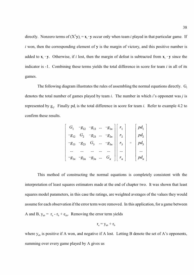
The following diagram illustrates the rules of assembling the normal equations directly. Gi

denotes the total number of games played by team i. The number in which i’s opponent was j is

represented by gij. Finally pdi is the total difference in score for team i. Refer to example 4.2 to

confirm these results.

This method of constructing the normal equations is completely consistent with the

interpretation of least squares estimators made at the end of chapter two. It was shown that least

squares model parameters, in this case the ratings, are weighted averages of the values they would

assume for each observation if the error term were removed. In this application, for a game between

A and B, yab = ra - rb + eab. Removing the error term yields

ra = yab + rb

where yab is positive if A won, and negative if A lost. Letting B denote the set of A’s opponents,

summing over every game played by A gives us

39

Gara = 3B (yab + rb)

Gara = pda + 3j�a gajrj

which is equivilent to the ath normal equation. Dividing by Ga reveals that ra is indeed an average

in which the weights are equal to either 0 if A did not participate in a game, or 12 = -12 = 1 if A did

play in the game.

What exactly is being averaged? For each game, the margin of victory and the opponent’s

rating are added to the total. This partial sum, yab + rb, is called the normalized score for team A.

It is an estimate of A’s performance in a particular game after controlling for the strength of the

opponent. Therefore a team’s rating is simply the average of its normalized scores. (Other work has

proposed using the median of normalized scores, instead of the mean, as the criterian for selecting

ratings (Bassett 1997). However, this would require us to abandon the least squares approach in

favor of minimizing the absolute error, 3ei = | yi - (ra - rb) |.)

This interpretation makes it evident that a team’s rating is directly impacted by not only its

average margin of victory, but also the level of competition it faced. In fact, a team’s rating is the

mathematical sum of its average margin of victory and its average schedule strength. Consequently,

least squares ratings are valuable in the sense that they go beyond wins and points to determine how

much respect a team really deserves for its performance. Success, especially against strong

opponents, translates into a high rating.

Once the normal equations have been derived, the unique solution is found by introducing

the scale and then solving the system, XTXr = XTy, for r. Calculating and then multiplying by

(XTX)-1 is both inefficient and unnecessary. Several methods of solving systems of simultaneous

linear equations are presented in chapter three. Small systems are usually solved directly with an

algorithm such as Gaussian elimination; the solution to a large system can generally be found more

40

quickly with an iterative procedure like the Gauss-Seidel method.

This concludes the description of the general least squares rating model. As mentioned

before, many alterations may be devised in order to tailor this model to emphasize other components

in the realm of sports competition. The following is by no means an exhaustive list of possible

modifications; however they serve as common examples that may be applied to the basic model to

generate more meaningful results.

Homefield Advantage

If an assumption is made that the home team in any game benefits by a fixed number of

points, then an additional variable can be attached to the general model:

Y = ra - rb + xhrh

The new independent variable xh indicates the location of the game. For example if xh = 1 then the

winning team A was the host; likewise if xh = -1 then A was the visitor. Of course varying degrees

of homefield advantage are possible, including a neutral site represented by xh = 0. The model

parameter rh becomes the universal homefield rating for the league in question. Universal refers to

the fact that each team experiences the same advantage when playing at home. It has been shown

in one study that such a null hypothesis cannot be rejected at standard statistical levels of

significance. Furthermore any indication of team to team differences in the homefield advantage is

relatively unimportant (Harville 1994).

Example 4.3

Let A’s rating equal 20 and B’s rating equal 18. In addition, assume a homefield constant

41

of 4 points. Then the expected outcome of a contest at A would favor A by (20-18+4) = 6 points.

However, B would be predicted to win by (18-20+4) = 2 points if it were the home team instead. #

Derivation of the normal equations is similar to the general case. You can verify that they

are equivalent to the following table:

Here Hi, i=1..n, denotes the difference in number of home and road games for team i. So if i played

7 games at home versus 5 as the visitor then Hi = 7-5 = 2. Gh represents the total number of games

in which one team benefited from the homefield advantage. Finally, pdh designates the total point

differential for home teams. Some modifications may be necessary if xh is allowed to assume values

other than 1, -1, or 0.

Notice that it would be possible to calculate both a home and away rating for each team,

permitting non-universal homefield advantages. However this would introduce unnecessary

complication to our model and conflict with the intent of deriving a single value to represent a team’s

strength.

Game Outcome Measure

Because of the intricacies of sports, including motivation and coaching philosophy, it could

42

be argued that a diminishing returns principle should be implemented in any rating model. This

strategy attempts to avoid the situation in which a team is rewarded for blowing out weak opponents,

an unfortunate characteristic of the general least squares method. This occurs because least squares

ratings are actually averages, and the mathmatical properties of means demand sensitivity to outlying

or extreme values. Since margin of victory is the only statistic upon which the ratings are based, a

team can improve its rating by running up the score. In reality this is usually done to impress fans,

the media, or, in the case of college sports, the voters for the top 25.

Conversly, it is possible for a team’s rating to decline unfairly after a solid victory over a

pathetic team because it didn’t win by enough points to compensate for the opponent’s weakness.

This is sometimes caused by the additive nature of least squares ratings. If A is predicted to beat B

by 30 points and B is likewise 30 points better than C, then we get an unrealistic expectation that A

would defeat C by 60 points.

Although it results in a loss of mathematical significance, more reasonable results may be

obtained by applying a diminishing return function to the least squares rating method. Such a

function stipulates that as the margin of victory increases, the benefit to the winner increases at a

slower rate. The function result replaces margin of victory as the dependent variable y of the

regression. An example would be the signed square root of the margin of victory. In this case the

difference between an 81 point win and a 36 point win is equivalent to the difference between a 4

point win and a 1 point loss.

The ultimate case of diminishing returns completely throws out any information about the

score of a game. Each win is treated as if it were by one point, so y = 1 no matter what. Hence, there

is no distinction between an 80 point massacre and a 1 point nail-biter. Teams that subscribe to the

43

“Just Win Baby” philosophy are rewarded because winning, especially against opponents who win,

yields a higher rating (Zenor 1995).

The term game outcome measure (GOM) has been coined to describe any function, including

those that exhibit diminishing returns, used to calculate the dependent variable y in a least squares

rating model (Leake 1976). It is based on the idea that it is impossible to accurately establish how

superior one team is to another from margin of victory alone. In theory, any concoction of game

statistics can be taken as variables from which to formulate the GOM, but usually only the score is

necessary. The GOM becomes a single numerical representation of a team’s performance in a game

relative to its opponent. The general least squares method is modified by replacing margin of victory

with the GOM result.

Usually the implementation of a function to discount blowout scores produces a set of ratings

that possesses a certain degree of “fairness” absent from the general ratings. Although an inverse

function can be derived to translate the new ratings back into a predicted outcome, the mathematical

legitimacy of these expected results is sacrificed. Despite this fact, these versions of least squares

regression may model reality more effectively than the original because they incorporate a knowledge

that the nature of sports is not entirely consistent with ideals assumed by regression methodology.

Offense / Defense

Once ratings have been calculated, it is often desirable to break them down into various

components. In particular we will consider two primary indicators of a team’s strength in most any

sport: offense and defense. So far only a measure of the difference between the winner and loser has

been used in our models. Consequently, if we say A should defeat B by 2 points, this does not

44

differentiate between an expected score or 108-106 or 4-2.

Instead of one equation, y = ra - rb, for each game we now incorporate two:

ya = oa - db

yb = ob - da

Each team is likewise associated with two independent variables in the model, oi and di representing

offense and defense. These variables can be interpreted as a team’s ability to score points and prevent

its opponent from scoring points respectively. It is assumed that the expected number of points that

A should score against B is equal to ya = oa - db.

Example 4.4

Assume A has an offensive rating of 34 and defensive rating of 7, while B has an offensive

rating of 40 with a defensive rating of -2. The average score of a game between the two would be

[34-(-2)] = 36 to [40-7] = 33. This prediction is superior to simply stating the expected margin of

victory which is equal to 3. #

A significant deterrent to finding offensive and defensive ratings is that the size of the system

has doubled. Furthermore, this requires 22 = 4 times the storing capacity for the normal equations

while the number of computations increases by a factor of approximately 23 = 8. Fortunately this

problem can be avoided. The solution is based on the inherent relationship between the general least

squares ratings and the corresponding sets of offensive and defensive ratings. First notice that the

following normal equations can be derived for the offense/defense model.

45

The total points scored for and against team i are denoted by pfi and pai respectively.

Any solution to the normal equations will also satisfy the following relationship, obtained by

adding the ith and (i+n)th equations together. For every i, i=1..n

Gi(oi + di) - 3j�i gij(oj + dj) = pfi - pai = pdi

An examination of this result reveals that setting each ri equal to oi + di causes this system of n

equations to be identical to the normal equations derived for the general least squares rating model.

This implies that a team’s overall strength can be expressed as the sum of its offensive and defensive

ratings. Therefore once r has been found, the task has been reduced to determining how much of the

total rating should be attributed to each category.

One way to accomplish this is to form another system using only the first n normal equations.

Using the relation ri = oi + di, the ith equation can be written as

Gioi - 3j�i gijdj = pfi

Gi (ri - di) - 3j�i gijdj = pfi

46

Gidi + 3j�i gijdj = Giri - pfi

Since r is already known, we have the nonsingular system:

which can be solved for the defensive ratings d. The offensive ratings can then be found directly by

setting o = r - d. Notice that if o and d constitute a solution then so do o + c, d + c where c =

(c,c,...,c) and c is a constant. This means that the ratings can be scaled arbitrarily. A logical choice

for c could be found by setting the restraint, 3i=1..n di = 0.

Example 4.5

Refer back to the league presented in example 4.2. Calculation of the offensive and defensive

ratings gives the following results:

Team Offense Defense Overall

Beast Squares 8.625 -0.875 7.750

Gaussian Eliminators 4.063 -1.188 2.875

Likelihood Loggers 2.625 1.625 4.250

Linear Aggressors 6.187 0.438 6.625

The overall rating is the sum of the offensive and defensive ratings. Notice that except for a constant

factor of -5.375, these ratings are identical to those found prior to the offense / defense breakdown.

47

By setting 3di = 0, the offensive ratings now indicate the number of points a team is expected to score

against an average defense.

It can be infered from this table that most of the Beast Squares’ strength comes from their

offense. In fact their defense is below average. The opposite is the case for the Likelihood Loggers,

while the Linear Aggressors appear to have a more balanced attack. A sample prediction might be

the Likelihood Loggers over the Gaussian Eliminators by the score of [2.625 - (-1.188)] = 3.813 to

[4.063 - 1.625] = 2.438. The Eliminators’ poor defense causes the Loggers to score more than usual,

while the Loggers’ defense is able to contain the more powerful Eliminator offense. The typical result

will be a low scoring game. #

Weighting Games

In reality, not every game bears the same significance, and this concept can be applied to the

calculation of ratings. For instance, playoff games and must win situations should be weighted more

than meaningless contests between teams out of contention or decimated by injury. The arguments

at the end of chapter two confirm that weights can be applied to a linear regression without sacrificing

the mathematical legitimacy of the results, which are still unbiased estimators.

Referring to chapter two, let A be a (m x n) matrix where aijxij defines the weight to be

attributed to the ith observation of the jth variable. Then the ratings are a solution to ATXr = ATy.

Unlike the general case, we cannot guarantee that a solution exists because ATX is not necessarily

symmetric. Hence it is possible to have a null vector of (ATX)T = XTA that is not a null vector of

(ATy)T = yTA. However, if we make a restriction that aijxij = aikxik whenever xij, xik � 0, then in this

model ATX will be symmetric and a solution can be found as before by introducing a scale to r.

48

Essentially this requirement states that a game result must carry the same significance for both teams.

Appropriate multipliers should be applied directly when constructing the normal equations.

Besides previously mentioned cases of weighting important games more than meaningless

contests, there are other situations in which this idea may be employed. For example more recent

games are usually better indicators of a team’s current strength, and therefore can be assigned more

emphasis in the least squares model. Also the concept of discounting games between overmatched

opponents can be addressed by weighting close games more than blowouts. The primary advantage

of such applications is that the results are still unbiased estimators, and thus predictions obtained from

the ratings are still valid from a statistical as well as logical perspective.

Summary

Although they have been presented individually, modifications to the general least squares

method can be used in combination with each other. Again, the beauty of this rating system is its

flexibility. See the appendix for some good comparisons of the ratings derived from selected variants

of the least squares model.

In addition, the results of several good implementations have been published, both in

statistical literature and informally on the internet. Leake (1976) described how least squares ratings

are analogous to the interaction of voltages in electrical networks. Other authors, such as Harville

(1977) and Stern (1996), have proposed modifications to the general model to better account for

natural variablility in team performance. These improved models permit more sophisticated

predictions and the computation of relevant confidence intervals. However, they require more

advanced statistical analysis of the distributions associated with rating parameters.

49

Chapter 5: Maximum Likelihood Ratings

Ratio and Percentage Rating Models

To a certain extent, the result of any sporting event can be described by one of two outcomes:

a win or a loss. Of course such an interpretation is relative to the team in question, since a win for

one team is necessarily a loss for the other. Without loss of generality, we may assume that ties

contribute half a win to each team. Notice also that we need not confine the definition of a “win”

to the traditional unit of a game. For example scoring a single point can be designated as a win, or

perhaps more appropriately as a success. Likewise, allowing an opponent to score a point could be

considered a loss, corresponding to a general instance of failure.

It is natural to assume that in a conceptually infinite series of contests between a pair of

teams, a certain proportion, p, of the wins or successes would be claimed by one team while the

remainder, 1-p, would belong to the other. This gives meaning to a statement such as “A has a 90%

chance of beating B.” Simply put, if the teams were to play ten games, then A would be expected

to win (0.9)(10) = 9 of them. Despite the high value of p, a victory for B is not impossible. Even

though it is obvious that A is a better team and has the potential to win every game, occasionally B

will prevail whether because of officiating, injury, weather, motivation, mental awareness, peaks in

physical performance, or some other arbitrary factor.

Although the exact value of p cannot be known, it can usually be approximated by

observations of prior outcomes. When more than two teams are involved, it is desirable to be able

to estimate pij for any given pair of teams. This should be possible even for teams who have either

never met or only played each other in a minimal number of contests. This chapter, as well as

50

chapter six, discusses rating systems that have been designed to satisfy these criteria.

Certain advantages are inherent in such rating methods. Obviously these include the ability

to easily estimate ratios and percentages, especially when referring to the winner of a game. A less

noticable benefit is that when some other measure of success, such as points scored, is employed,

defensive teams do not suffer from an unfair bias towards powerful offenses, which often result in

higher margins of victory despite a possibly lower success ratios. As an illustration, consider scores

of 50-20 and 21-3. An unmodified version of least squares would discriminate in favor of the larger

margin of victory. In contrast, the ratio or percentage models described in this unit naturally assign

considerably more authority to the 21-3 effort. Unfortunately this feature requires a tradeoff. Since

a given percentage does not distinguish among levels of scoring, it becomes less practical to estimate

margin of victory or predict a game score with these rating models.

The M.L.E. Model

Probability rating models assume that for any given game between two teams, A and B, there

is a certain probability, p, that A will win. Ignoring ties, the corresponding probability that B will

win is equal to 1-p. This defines the result of each game as a random variable Xi having the

Bernoulli distribution with parameter p, 0# p# 1. In reference to team A, if we let the value of a win

equal 1 and a loss equal 0, then Pr(Xi=1) = p and Pr(Xi=0) = 1-p.

If A and B play each other g times, we will assume that these games’ outcomes have

identical and independent Bernoulli distributions with parameter p. These random variables form

g Bernoulli trials, and if we let X = 3i=1..g Xi then X will have a binomial distribution with

51

parameters g and p (Degroot 1989). The probability density function (p.d.f.) of X is given by:

(1)

The value of this function at x can be interpreted as the probability that A would win x out of g

games against B.

When an entire league of n teams is under consideration, a similar random variable Xij is

defined for each pair of teams, i and j. These variables all have binomial distributions based on the

number of games the two teams play against each other, gij, and the probability, pij, that i would

defeat j in any particular game. The corresponding probability density function, fij, has the following

representation, analogous to equation 1:

(2)

Individually, each fij describes one particular series of games between two teams by assigning

probabilities to the possible results that could be observed. If we continue to assume independence,

then these p.d.f.’s can be multiplied together to form a joint distribution that incorporates the entire

league at once.

(3)

Example 5.1

Consider a league consisting of three teams in which the probability of A defeating B is pab

= 0.6, the probability of A defeating C is pac = 0.8, and the probability of B defeating C is pbc = 0.7.

52

Therefore p = (0.6, 0.8, 0.7). Corresponding to g = (2, 1, 3) is the schedule in which A plays B

twice, A plays C once, and B plays C three times. Consequently the joint probability density

function for this situation is given by

To calculate the probability that A and B would split, A would defeat C, and B would win two out

of three against C, evaluate f at x = (1, 1, 2). The result is 0.169, so there is a 16.9% chance that this

particular set of outcomes would occur. Notice that the various orders in which games could be won

or lost is not important. #

Each set of possible results for any given schedule of games in the league is now assigned

a probability of occurring by the joint p.d.f. in equation 3. However in order to compute the value

of f, we must first know every probability pij of one team defeating its opponent in a particular

contest. Unfortunately this information is generally not available. In fact, the purpose of this rating

system is to estimate these probabilities. We wish to choose a vector of ratings, r, such that it is

possible to express pij as a function of ri and rj. A prediction function, p(ri, rj), serves to narrow the

possible values of pij, and in the process causes the estimated probabilities to be consistent and valid

for any pair of teams. Consequently, it is not limited to those teams that have considerable previous

experience playing against each other.

Ratings must first be defined in terms of how they will be interpreted when determining

probabilities. A suitable choice is to let

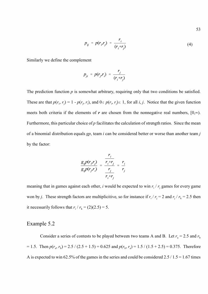
53

(4)

Similarly we define the complement

The prediction function p is somewhat arbitrary, requiring only that two conditions be satisfied.

These are that p(ri, rj) = 1 - p(rj, ri), and 0# p(ri, rj)# 1, for all i, j. Notice that the given function

meets both criteria if the elements of r are chosen from the nonnegative real numbers, [0,4).

Furthermore, this particular choice of p facilitates the calculation of strength ratios. Since the mean

of a binomial distribution equals gp, team i can be considered better or worse than another team j

by the factor:

meaning that in games against each other, i would be expected to win ri / rj games for every game

won by j. These strength factors are multiplicitive, so for instance if ri / rj = 2 and rj / rk = 2.5 then

it necessarily follows that ri / rk = (2)(2.5) = 5.

Example 5.2

Consider a series of contests to be played between two teams A and B. Let ra = 2.5 and rb

= 1.5. Then p(ra, rb) = 2.5 / (2.5 + 1.5) = 0.625 and p(rb, ra) = 1.5 / (1.5 + 2.5) = 0.375. Therefore

A is expected to win 62.5% of the games in the series and could be considered 2.5 / 1.5 = 1.67 times

54

stronger than B. #

If the functional representation of pij in equation 4 is substituted into the binomial distribution

in equation 2 then we have

The product of all such independent p.d.f.’s form the joint distribution in equation 3. After

collecting terms and simplifying, we have

(5)

Here C equals the product of all combination constants, . Also, wi = 3j=1..n xij denotes the total

number of wins for team i.

The multivariable joint distribution function in equation 5 assigns a probability to any

specific set of game outcomes x that could occur given the schedule g and the teams’ ratings r. In

particular, we wish to consider the value of this function using the results of completed games, which

in essence is the prior probability that exactly those outcomes would have occurred. However, the

rating vector r must necessarily be considered a set of n unknown parameters, one for each team.

It is the purpose of this discussion to develop some means of estimating r based on the actual

observations, which ideally should be evidence of where the true ratings are likely to lie.

55

Assuming that each team plays at a level indicitive of its true ability, it seems logical to

believe that a good estimate of r should yield a relatively high probabilitiy from equation 5 when x

corresponds to observed game results. This means that the actual game outcomes would not be

considered unlikely if in fact they were generated by teams with those ratings. Conversely, a lower

value for f would seem to suggest that some of the ratings are not accurate because they require an

uncharacteristically large number of “upsets.” In summary, choosing the estimates to best reflect

reality can be accomplished by maximizing f for the given x. Each determined in this manner is

called a maximum likelihood estimator (DeGroot 1989).

Example 5.3

Assume that A defeated B in a five game series, 4-1. The p.d.f. evaluated at x = 4 is:

If ra = 2 and rb = 1 then f(4) is equal to 0.329. However if ra = 4 and rb = 1 then f(4) increases to

0.410. This can be interpreted as meaning that the latter rating estimates are more likely to have

produced the observed outcomes. In fact, it can be shown that the ratio, ra / rb = 4, will yield the

highest possible value for f. #

When a joint p.d.f. is regarded as a function of one or more parameters for a given x, it is

called the likelihood function, which is typically denoted by L (DeGroot 1989). In a sense, the

unknown rating parameters become variables, a conversion made possible because the observed x

is now treated as a constant. Although it is not itself a p.d.f., the likelihood function defines relative

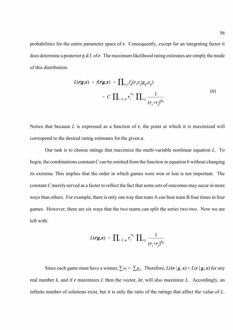
56

probabilities for the entire parameter space of r. Consequently, except for an integrating factor it

does determine a posterior p.d.f. of r. The maximum likelihood rating estimates are simply the mode

of this distribution.

(6)

Notice that because L is expressed as a function of r, the point at which it is maximized will

correspond to the desired rating estimates for the given x.

Our task is to choose ratings that maximize the multi-variable nonlinear equation L. To

begin, the combinations constant C can be omitted from the function in equation 6 without changing

its extrema. This implies that the order in which games were won or lost is not important. The

constant C merely served as a factor to reflect the fact that some sets of outcomes may occur in more

ways than others. For example, there is only one way that team A can beat team B four times in four

games. However, there are six ways that the two teams can split the series two-two. Now we are

left with:

Since each game must have a winner, 3wi = 3gij. Therefore, L(kr | g, x) = L(r | g, x) for any

real number k, and if r maximizes L then the vector, kr, will also maximize L. Accordingly, an

infinite number of solutions exist, but it is only the ratio of the ratings that affect the value of L.

57

Because any element, ri , of r can be scaled to a specified value by choosing an appropriate k, a

unique solution can be obtained by setting some element of r equal to a constant, leaving a function

of n-1 variables. For simplicity, rn will be set equal to one. In essence, this creates a standard by

which all other teams are measured by.

To determine the extrema of L, it is necessary to find the point at which the partial derivatives

ML / Mri = 0 for i= 1..n-1. In its current form, it would be very difficult and time consuming, even for

a computer, to arrive at expressions for the partial derivatives of L. However, because L $ 0 for all

r, and the natural log, ln(x), is an increasing function of x, the function � = ln(L) will be maximized

at the same point for which L is maximized. The use of a log likelihood function greatly simplifies

our work because by taking advantage of logarithmic laws, � can be expressed as a sum rather than

a product.

(7)

Except for the boundaries, any critical point of � must be a solution to the following non-linear

system of equations, obtained by setting the partial derivatives of � equal to zero:

(8)

Furthermore, we can choose a constant, 0 < c < min (ri, i=1...n ), such that for i=1...(n-1),

58

Since the second derivatives are all negative, we have reason to believe that a solution to the

system must yield a local maximum for �, and hence also for L. Certainly there is no local

minimum, so the absolute maximum for � must occur at either a boundary point or at the solution

to equation 8. In order to use the log likelihood function, it must be assumed that no ri equals zero.

As long as each team has at least one win, this condition is met. Similarly, if each team has at least

one loss then ri cannot be infinite. Therefore we can infer that a solution, , to the system must yield

an absolute maximum for the likelihood function. These ratings comprise the set of maximum

likelihood estimators for the distribution.

Example 5.4

Suppose the following results were observed in a certain league of four teams.

Beast Squares defeat Gaussian Eliminators 10-6

Likelihood Loggers tie Linear Aggressors 4-4

Linear Aggressors defeat Gaussian Eliminators 9-2

Beast Squares defeat Linear Aggressors 8-6

Gaussian Eliminators defeat Likelihood Loggers 3-2

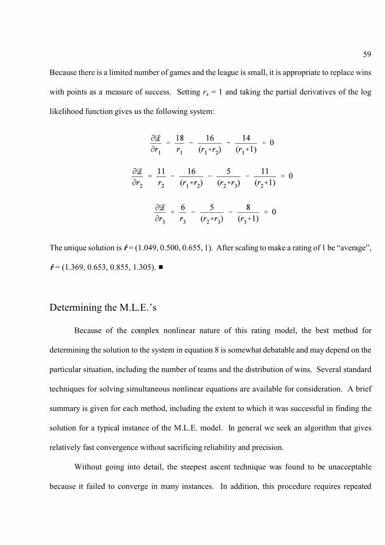
59

Because there is a limited number of games and the league is small, it is appropriate to replace wins

with points as a measure of success. Setting r4 = 1 and taking the partial derivatives of the log

likelihood function gives us the following system:

The unique solution is = (1.049, 0.500, 0.655, 1). After scaling to make a rating of 1 be “average”,

= (1.369, 0.653, 0.855, 1.305). #

Determining the M.L.E.’s

Because of the complex nonlinear nature of this rating model, the best method for

determining the solution to the system in equation 8 is somewhat debatable and may depend on the

particular situation, including the number of teams and the distribution of wins. Several standard

techniques for solving simultaneous nonlinear equations are available for consideration. A brief

summary is given for each method, including the extent to which it was successful in finding the

solution for a typical instance of the M.L.E. model. In general we seek an algorithm that gives

relatively fast convergence without sacrificing reliability and precision.

Without going into detail, the steepest ascent technique was found to be unacceptable

because it failed to converge in many instances. In addition, this procedure requires repeated

60

evaluations of the function in equation 7. Besides being costly in terms of time, these calculations

were found to be limited in their accuracy, especially for large systems.

An unoptimized implementation of Newton’s method also exhibited erratic performance.

However, when convergence was achieved, it required relatively few iterations compared to other

methods. Usually divergence was caused by the tendency of the ratings to grow without bound with

each successive iteration. An explanation for this phenomenon is suggested by the following

diagram:

This is a typical graph of the partial derivative of ri assuming that the other ratings are held constant

at their current approximated values r(k-1). The desired rating is at the intersection p. Notice the

horizontal asymptote, . Since Newton’s method follows the tangent line out to its

intersection with the axis, an initial value of ri(k-1) greater than the critical point q will cause the the

subsequent approximation ri(k) to approach infinity instead of the desired point p. Divergence may

also be caused when ri(k-1) is only slightly less than q, causing the next estimate to be negative, in

violation of the model definition.

To correct these behaviors, a modified Newton’s method was constructed that adjusts only

one rating parameter at a time. This is possible because the second partial derivatives,

are relatively insignificant when i�j. Besides allowing the justification of each move, this revised

61

procedure circumvents the construction and solution of a (n x n) jacobian matrix. The

implementation can be described by:

where and . The first condition guarantees that the next estimate

ri(k) will not shoot out towards infinity, while the second condition prevents negative values for ri

(k).

In either case, ri(k-1) is too large so we can divide by a constant c. For best results, choose 1# c# 2.

Experience has shown that this modified Newton’s method consistently converges in a reasonable

amount of time.

Fixed point iteration is perhaps the simplest and most reliable method of solving non-linear

systems. To utilize the fixed point method a function h, mapping ún-1 into ún-1, must be constructed

such that h(r) = r whenever r is a solution to the system in equation 8. This condition can be

satisfied by defining h(r) = (h1(r), h2(r), ... , hn-1(r)) where

(9)

A sequence {r(k)}k=0...4 can be generated by selecting an arbitrary r(0) and letting r(k) = h(r(k-1) ). If this

sequence converges to a point r, then r must be a fixed point of h and therefore a solution to equation

8 since:

r = limk64 r(k) = limk64 h(r(k-1) ) = h(limk64 r

(k-1) ) = h(r)

62

Modestly accelerated convergence may be obtained with Seidel’s method, which simply

involves using the most recent values for r1(k)...ri-1

(k) when computing ri(k). For this model,

surprisingly significant improvement can also be achieved by allowing rn to “float”, instead of

holding it as a fixed constant. The function h becomes n-dimensional with hn(r) having the same

form as equation 9, allowing the nth rating to be adjusted as necessary with each iteration. Eventually

the resulting sequence will settle at one particular solution. Once convergence is reached, the ratings

can be scaled arbitrarily.

The fixed point method almost always produces a solution, especially for a good initial

approximation r(0). A logical choice for ri(0) is simply team i’s ratio of wins to losses, wi / li. Because

of its self-correcting nature, fixed point iteration can be continued until the desired precision is

reached, limited only by the floating point accuracy of the computer. Although it exhibits only linear

convergence, the fixed point algorithm can be implemented very easily. Each iteration requires

significantly fewer calculations than variants of Newton’s method or other more sophisticated

techniques. As a result, the total time required compares favorably. The combination of consistency,

precision, and speed makes fixed point iteration the method of choice for this rating model

application.

Change of Variables

As was mentioned earlier, the prediction function upon which M.L.E. ratings are based is not

necessarily unique. Until now we have dealt with only one example, namely p(ri, rj) = ri / (ri + rj).

Algebraicly, this is probably the simplest form that meets both criteria required of the prediction

function. However other possiblities exist that may offer certain advantages despite being slightly

63

more complex.

The following derivation is largly intuitive, depending on some basic concepts about a team’s

winning percentage. It is assumed that a 0.500 team is considered average. Furthermore we can

interpret a 0.750 team to have a 75% chance of winning a game against an average team. More

generally, a team with p winning percentage should win 100p percent of its games against a typical

opponent.

A more interesting situation occurs when neither team in a particular game is “average.” For

example if A is a 0.750 team and B is a 0.600 team, what is the probability that A defeats B?

Although it is obviously not true, we can assume for the moment that the odds of A winning are

independent of B winning. Therefore we have the following possible scenarios:

P(both A and B win) = (0.750)(0.600) = 0.45

P(A and B lose) = (0.250)(0.400) = 0.10

P(A wins and B loses) = (0.750)(0.400) = 0.30

P(B wins and A loses) = (0.250)(0.600) = 0.15

Now it is impossible for both teams to win or lose the same game. Therefore we only need to

consider the final two probabilities. Since the total probablility must total one, a scale must be

introduced to condition for the only results that are feasible (Woolner 1996). In particular, we can

now conclude based on the assumptions that A has a (0.30) / (0.30 + 0.15) = 0.667 chance of

defeating B. If we generalize this procedure to account for two arbitrary winning percentages pa and

pb, then

64

For a league in which each team has played an identical schedule, the preceding formula is

valid. However this would be quite unusual. To compensate, the winning percentages can be

replaced by ratings. The domain for the teams’ ratings is the same as for their winning percentages,

[0,1]. Therefore, given two teams, we can determine the probable outcome from their ratings and

the following prediction function, which serves the same purpose as equation 4.

(10)

A likelihood function for the rating parameters r can be constructed as before, with equation 10

replacing equation 4. Although it may entail more complicated calculations, determining the set of

M.L.E.’s is analogous to the procedures outlined earlier in this chapter, with the only difference

being the definition of the prediction function.

By dividing both the numerator and denominator by (1-ri)(1-rj), equation 10 can be rewritten

as

where h(ri) = ri / (1-ri). The form of this equation in terms of the function h is identical to the

original prediction function in equation 4, p(ri, rj) = ri / (ri + rj). Since we are able to find maximum

likelihood estimators for r using either function as the base, it seems logical to look for some

relationship between the two resulting sets of M.L.E.’s. For clarity, the ratings and M.L.E.’s

65

obtained with the prediction function in equation 10 will be denoted by s and , while those obtained

with equation 4 will still be expressed as r and . Therefore we can write h(si) = si / (1-si).

Notice that h is an injective function from the domain of si to the domain of ri, h:[0,1]6[0,4).

If we let ri = h(si), then equation 10 is transformed into equation 4 by this change of variables.

Furthermore the invariance property of maximum likelihood estimators implies that if is the

M.L.E. of si then h( ) is the M.L.E. of h(si) (DeGroot 1989). Therefore if is known then can

easily be calculated by simply setting each = h( ) = / (1- ). Because h is one to one, its

inverse function, g(ri) = h-1(ri) = ri / (ri + 1), provides an equivalent method of determining from

.

We have just established that the two sets of M.L.E.’s, and , are essentially equivalent;

knowing one is sufficient to determine the other. An additional implication is that the predictions

obtained from either vector of ratings estimators will always be identical. This follows because the

relationship between any two teams’ ratings is preserved relative to the prediction function used to

generate them. In fact, this is the case for any prediction function that can be written as

for some injective function g.

A change of variables, such as from r to s, offers several important advantages. First we have

accomplished a mapping from the infinite scale [0,4) to a finite one, [0,1]. This not only prevents

computer overflow, but also provides a more interpretable set of ratings. Most sports fans can easily

understand the differences between a 0.750 team and a 0.500 team. However they would likely find

it more difficult to compare teams with ratings 3 and 1 respectively. In addition, ratings from s can

be scaled to be symmetric, so that a 0.250 team is as bad as a 0.750 team is good. This is in contrast

to r, for which 0.333 and 3 are complements. One final benefit of a change of variables is that it may

66

facilitate solving for the M.L.E.’s. For example, Newton’s method often converges faster when the

likelihood function is based on equation 10. More research is necessary to determine what choices

for g(ri) would cause the most improvement.

Modifications

Although the M.L.E. rating model has a strong statistical foundation, it is often cumbersome

to work with. This especially applies when we wish to modify it to account for homefield advantage

or other factors important in sports. Usually this will require a complete re-formulation of the

likelihood function, and also the nonlinear system that must be solved. It is suggested that more

research be done in these situations to decide how one should proceed in determining the solution

from an algorithmic perspective.

Another possible avenue of research is to consider the use of a mean or median instead of the

mode as a criterian for determining ratings. By definition, the M.L.E. ratings seek the point at which

the probability of the observed results is maximized. However, consider the simple problem when

team A defeats team B in a single game. Obviously we would not expect A to win every game

against B, but this is exactly the implication of the resulting M.L.E. ratings. A better approach may

be to determine an average rating, based on some Bayesian prior probability distribution.

Preliminary experiments indicate that the implementation of such a model requires significant use

of numerical integration within a framework analogous to a neural network (Harris 1996).

67

Chapter 6: The Elecs Rating Method

Introduction

The Elecs rating model was developed by Dr. Eugene Potemkin, who first applied the

techniques to international sporting events such as the Olympics, World Cup Soccer, and the Chess

Olympiad. A resident of Moscow, Dr. Potemkin has published his results in the Russian press since

the early 1980's under the moniker “Elecs,” short for “Electronic System.” Recent access to the

internet has allowed him to introduce the Elecs method to American sports. The following

descriptions have been adapted from my email correspondence with Dr. Potemkin in relation to our

joint effort, the “World Wide Ratings and Rankings” web site.

Despite its dependence on mathematical formulas, the Elecs method was not originally

intended to generate ratings that satisfy some strict mathematical criteria or conform to standard

statistical procedures. Instead, Dr. Potemkin’s motivation for developing this particular rating

system was more of a pragmatic nature, based on intuition and a general knowledge of sports

competition. However with the proper interpretation it can be shown that the Elecs model is an

application of continuous time Markov chains, a class of probability models. This chapter will focus

primarily on Dr. Potemkin’s derivation and its practical connection with economic theory; the

equivalence to Markov chains is briefly described at the end of this chapter.

The Elecs Model

Like maximum likelihood ratings, the Elecs system is designed to model probabilities. In

particular, the ratio of two teams’ ratings should approximate , the ratio of games won by A

68

to those won by B in a conceptually infinite series of contests between the two teams. Ties may be

assumed to contribute half a win to each team. A pair of “Binary Ratings,” brij and brji, can be

chosen to represent the win ratio in games between team i and any one of its opponents j. Notice that

binary ratings are not fixed numbers because they represent only a ratio; however the relationship

between two binary ratings can be established. We set

brijwji = brjiwij

brijwji + brijwij = brjiwij + brijwij

brijgij = wij(brij + brji)

(6.1)

where gij = wij + wji equals the total number of games played between i and j. This implies that the

strength attributed to a team via a binary rating is directly proportional to the percentage of games

it won, and also to the total binary rating for both teams. So far, the binary ratings have no relation

to actual team ratings; they are only relevant when describing the relationship between an isolated

pair of teams.

Each team will have as many binary ratings as it has opponents. The goal will be to calculate

a vector of general ratings r from which to estimate binary ratings for teams that have never met.

A logical choice for a team’s general rating is the average of its known binary ratings. Therefore we

define the rating for each team i, i=1..n, to be

69

where gi is the total number of games played by team i. Substituting equation 6.1 gives us

For a particular contest, it is generally impossible to determine whether variation in the

outcome should be explained by one team’s above average performance or the other team’s below

average performance. To quote Dr. Potemkin, “Each team plays the way her opponent lets it play.”

Consequently, an assumption made by the Elecs model that is not likely to be unrealistic is that

ri - brij = -(rj - brji)

ri + rj = brij + brji (6.2)

This simply states that the binary ratings for a single game will total the sum of the participant’s

overall ratings. Although this relationship is not entirely correct mathematically because of the

nonlinear nature of ratios, it serves as a satisfactory estimate for our purposes.

Example 6.1

Suppose A’s rating equals 5 and B’s rating equals 2. Then A is expected to win 5/2 games

for every 1 game won by B. Now assume that A defeated B in three of the five games played

between the two teams. The appropriate values would be brab = 4.2 and brba = 2.8. Notice that brab

+ brba = 7 and brab / brba equals the correct win ratio, 3 / 2. #

70

Based on equation 6.2, the general Elecs model can be formulated as

This results in a set of n linear equations of the form

giri - wiri = 3i�jwijrj

liri = 3i�jwijrj (6.3)

where wi and li equal the number of wins and losses respectively by team i. Exactly n-1 of these

equations will be independent because li = 3j�iwji for all i. This should be expected since for any real

number c, cr yields ratios equivalent to those obtained from r. Therefore an arbitrary condition can

be imposed on the solution. A logical choice would be to set 3ri = c for some positive number c.

Another possibility could be to make the ratings relative to one particular team k by setting rk = 1.

The Elecs ratings exhibit certain characteristics based on the model definition. First we

notice that each ri will be nonnegative. Zero ratings are possible, occurring if a team has no wins

against any of its opponents. In the opposite case, if a team is undefeated, then the model breaks

down. Depending on the conditions set by the nth equation, two results are possible. Either ratings

for teams that did lose will become zero, or those that didn’t will be infinite. This is a significant

weakness of the Elecs method and ratio models in general. Consequently, measures should be taken

to insure that no li equals zero. Replacing wins with points will usually solve the problem. An

alternate proposal would be to weight the results with an adjustable parameter x, 0#x#1. A single

win would then be treated by the model as x wins and (1-x) losses.

71

As with least squares ratings, it is assumed that enough games have been played to produce

a saturated system in which each team has some connection with every other team in the league. The

final system of linear equations in the Elecs model can be solved with the techniques discussed in

chapter three. A solution can usually be obtained more efficiently than for nonlinear ratio models.

This advantage may offset the sacrifice of mathematical legitimacy caused by the linear

approximation of an inherently nonlinear design.

Example 6.2

Consider the league referred to in example 4.2 and assume the following results:

Beast Squares defeat Gaussian Eliminators 10-6

Likelihood Loggers tie Linear Aggressors 4-4

Linear Aggressors defeat Gaussian Eliminators 9-2

Beast Squares defeat Linear Aggressors 8-6

Gaussian Eliminators defeat Likelihood Loggers 3-2

Replacing wins with points and constructing the system of equations defined by equation 6.3 yields

This system is obviously singular, so we introduce the restraint that 3ri = 4.

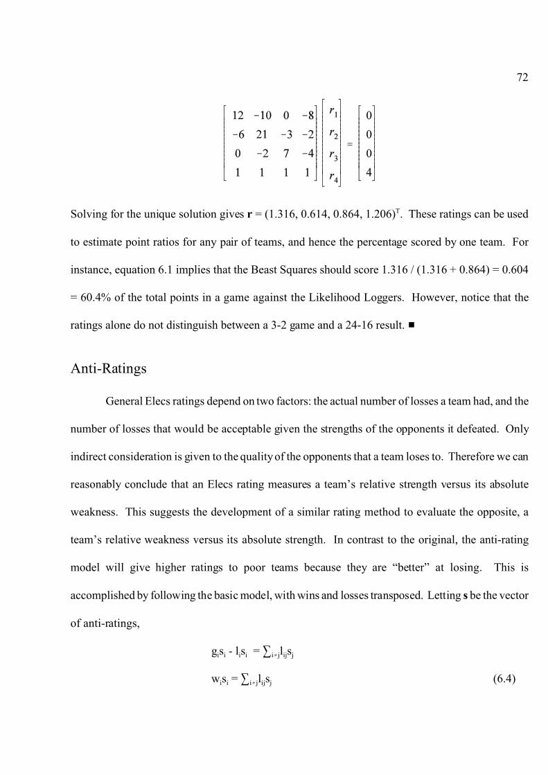
72

Solving for the unique solution gives r = (1.316, 0.614, 0.864, 1.206)T. These ratings can be used

to estimate point ratios for any pair of teams, and hence the percentage scored by one team. For

instance, equation 6.1 implies that the Beast Squares should score 1.316 / (1.316 + 0.864) = 0.604

= 60.4% of the total points in a game against the Likelihood Loggers. However, notice that the

ratings alone do not distinguish between a 3-2 game and a 24-16 result. #

Anti-Ratings

General Elecs ratings depend on two factors: the actual number of losses a team had, and the

number of losses that would be acceptable given the strengths of the opponents it defeated. Only

indirect consideration is given to the quality of the opponents that a team loses to. Therefore we can

reasonably conclude that an Elecs rating measures a team’s relative strength versus its absolute

weakness. This suggests the development of a similar rating method to evaluate the opposite, a

team’s relative weakness versus its absolute strength. In contrast to the original, the anti-rating

model will give higher ratings to poor teams because they are “better” at losing. This is

accomplished by following the basic model, with wins and losses transposed. Letting s be the vector

of anti-ratings,

gisi - lisi = 3i�jlijsj

wisi = 3i�jlijsj (6.4)

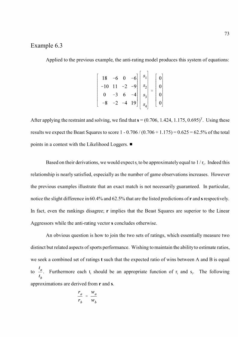
73

Example 6.3

Applied to the previous example, the anti-rating model produces this system of equations:

After applying the restraint and solving, we find that s = (0.706, 1.424, 1.175, 0.695)T. Using these

results we expect the Beast Squares to score 1 - 0.706 / (0.706 + 1.175) = 0.625 = 62.5% of the total

points in a contest with the Likelihood Loggers. #

Based on their derivations, we would expect si to be approximately equal to 1 / ri. Indeed this

relationship is nearly satisfied, especially as the number of game observations increases. However

the previous examples illustrate that an exact match is not necessarily guaranteed. In particular,

notice the slight difference in 60.4% and 62.5% that are the listed predictions of r and s respectively.

In fact, even the rankings disagree; r implies that the Beast Squares are superior to the Linear

Aggressors while the anti-rating vector s concludes otherwise.

An obvious question is how to join the two sets of ratings, which essentially measure two

distinct but related aspects of sports performance. Wishing to maintain the ability to estimate ratios,

we seek a combined set of ratings t such that the expected ratio of wins between A and B is equal

to . Furthermore each ti should be an appropriate function of ri and si. The following

approximations are derived from r and s.

74

Hence we can establish the relationship

Setting ti = (ri / si)½ the following condition is met.

Example 6.4

Combining the results of examples 6.2 and 6.3 gives the following table:

Team Rating (r) Anti-Rating (s) Overall (t)

Beast Squares 1.316 0.706 1.365

Gaussian Eliminators 0.614 1.424 0.657

Likelihood Loggers 0.864 1.175 0.858

Linear Aggressors 1.206 0.695 1.317

The Beast Squares should therefore win 1.365 / (1.365 + 0.858) = 0.614 = 61.4% of games against

the Likelihood Loggers, a proper compromise between the two prior estimates. #

Economics Approach

The Elecs model is quite similar to the economic principles of supply and demand. We can

consider our league as a marketplace in which teams exchange products, which correspond to games.

If a team wins then it in effect purchases a game from the loser, who receives compensation equal

75

to the price for that game. The primary goal is to calculate equilibrium prices for each team’s games.

Corresponding to the basic Elecs model is a sellers’ market, meaning that each team sets the

price for its own games. Ratings will coincide with prices, so the total expenses for a particular team

i is expressed as 3j�iwijrj. Equilibrium will occur when each team’s income equals its expenses so liri

= 3j�iwijrj, which is identical to the system defined by equation 6.3. From this model we can conclude

that a team creates demand for its games by winning, especially against “wealthy” opponents. Price

is proportional to the ratio of demand and supply, so from the league’s perspective a total of 3j�iwijrj

losses are demanded from team i; however only li are supplied. Consequently as supply decreases or

demand increases, a win against team i becomes more valuable and expensive to purchase.

The anti-rating model parallels a buyers’ market in which the purchaser of a game determines

how much it is willing or able to pay. Total income is then dependent on what the customers can

afford, expressed as 3j�ilijsj. Accordingly, equilibrium will occur when wisi = 3j�ilijsj, which matches

equation 6.4, is satisfied for each team. From team i’s perspective, it desired a total of 3j�ilijsj wins

and was able to purchase wi. Therefore, as supply increases or demand decreases, each of i’s wins

becomes worth less. This indicates that i is a strong team with an abundance of “wealth” such that

success is taken for granted.

Markov Chain Equivalence

It was mentioned earlier that the Elecs rating system is actually an application of continuous

time Markov chains. To see this, imagine that each team represents a possible state of the system,

which corresponds to the league as a whole. Furthermore, if the system is in state i, then this indicates

that team i recorded the most recent success, in terms of either winning a game or scoring a point.

76

Now if some opponent j comes along and defeats i, then the system transfers to state j. This process

continues indefinitely as teams fight for control of the system. Eventually equilibrium will be reached,

and it will be possible to state the exact probability that the system will be in a particular state at any

instant in time. With the proper model definition, these probabilities are proportional to the Elecs

ratings.

Without going into a detailed description of Markov chains, we will assume that transitions

from team to team are instantaneous. In addition, the rate at which transitions occur from team i to

team j is equal to the number of losses i had to j. Letting Q denote the transition rate matrix, we see

that qij = lij = wji. It can be shown that under the assumptions associated with continuous time Markov

chains, qii = -3j�i qij (Stewart 1994). This is essentially a measure of how often a team is forced to give

up control of the system. As expected, this occurs whenever that team loses. Therefore qii = -li.

Consider the example from example 6.2. The resulting transition rate matrix is

Equilibrium probablities p are a solution to pQ = 0, where 3 pi = 1. You can verify that p = (0.329,

0.154, 0.216, 0.301) satisfies these conditions. Also notice that p = 0.25r where r is the set of Elecs

ratings. Therefore except for a constant factor, the Elecs rating method is equivalent to the application

of a continuous time Markov chain. Of course, the reversal of wins and losses provides a similar

correspondence to anti-ratings.

77

Appendix

By far the most popular sports ratings are those done for college football. This is probably

because no playoff system has been initiated to decide the national championship. Instead, this

responsibility is given to the Associated Press and CNN / USA Today Coaches’ polls. Not

surprisingly, many rating models have been developed to help settle (or evoke) controversy among

college football fans.

The following two pages contain the results of rating models presented in this paper. They

are based on all division 1-A games played during the 1996 season. Games played outside division

1-A were ignored when calculating the ratings. In all, 111 teams are included. However, only the

top 25 are included in the tables. I must thank usatoday.com for providing easy access to the scores

and homefield data.

Table 1 contains the ratings from various least squares models. The numbers in parenthesis

are the rankings. The first column (LS) is the basic least squares system. Next (LSW) are the results

when each game is treated as a one point win. The third column (LSD) is based on an arbitrary

diminishing returns function: y equals the square root of the margin of victory plus a five point bonus

for winning the game. Finally, the (LSH) column factors in a homefield advantage, which turns out

to be about 3.5 points. The (Off) and (Def) breakdown of these homefield ratings is shown last.

Table 2 summarizes the results of several ratio models. The first column (MLE) contains the

results of the maximum likelihood system. After transferring to the finite scale [0,1], they can be

expressed as (Alt). Next are the Elecs ratings and anti-ratings, followed by the combination (Comb)

discussed in chapter six. Last are the final rankings from the major polls. It is interesting to notice

that both ratio models, M.L.E. and Elecs, imply that the national championship was awarded to the

wrong team.

78

Division 1-A College Football 1996 - Least Squares Ratings

Homefield Advantage = 3.593 points

Team LS LSW LSD LSH Off Def

Florida (12-1) 37.34 (2) 1.31 (1) 13.13 (1) 35.40 (2) 50.56 10.41

Ohio St. (11-1) 35.85 (3) 1.16 (3) 11.82 (2) 34.92 (3) 41.83 18.65

Florida St. (11-1) 30.41 (4) 1.18 (2) 11.52 (3) 28.83 (5) 40.17 14.22

Arizona St. (11-1) 30.39 (5) 1.02 (4) 10.46 (5) 29.21 (4) 43.50 11.27

BYU (14-1) 15.19 (19) 0.73 (14) 6.79 (17) 15.37 (18) 36.11 4.82

Nebraska (11-2) 38.86 (1) 0.95 (5) 10.79 (4) 38.09 (1) 45.51 18.14

Penn St. (11-2) 22.44 (9) 0.87 (8) 8.60 (8) 21.57 (9) 34.55 12.58

Colorado (10-2) 21.61 (11) 0.93 (6) 9.03 (6) 20.81 (11) 33.36 13.02

Tennessee (10-2) 23.62 (7) 0.88 (7) 8.64 (7) 22.02 (8) 38.51 9.07

North Carolina (10-2) 22.80 (8) 0.83 (9) 8.44 (9) 22.50 (7) 32.58 15.49

Alabama (10-3) 13.71 (23) 0.82 (10) 7.08 (14) 12.47 (23) 27.06 10.97

Virginia Tech (10-2) 15.00 (20) 0.77 (13) 7.12 (12) 14.04 (20) 31.57 8.03

LSU (10-2) 11.32 (27) 0.79 (12) 6.52 (19) 9.49 (29) 29.00 6.06

Miami (9-3) 13.96 (22) 0.68 (19) 6.31 (20) 13.50 (22) 31.80 7.26

Washington (9-3) 21.89 (10) 0.81 (11) 8.13 (10) 21.14 (10) 36.62 10.09

Northwestern (9-3) 8.96 (34) 0.61 (22) 5.07 (22) 8.83 (34) 30.90 3.49

Kansas St. (9-3) 17.16 (15) 0.70 (15) 6.85 (15) 16.91 (14) 28.22 14.25

Iowa (9-3) 16.42 (16) 0.69 (17) 6.52 (18) 15.69 (16) 31.46 9.79

Syracuse (9-3) 20.63 (12) 0.66 (21) 7.11 (13) 20.01 (12) 37.33 8.24

Michigan (8-4) 17.50 (14) 0.69 (18) 6.82 (16) 16.59 (15) 27.45 14.70

Notre Dame (8-3) 26.38 (6) 0.66 (20) 7.44 (11) 24.88 (6) 39.64 10.80

Wyoming (10-2) 7.49 (37) 0.35 (32) 3.18 (35) 7.58 (38) 33.39 -0.25

Texas (8-5) 19.24 (13) 0.40 (28) 4.93 (23) 18.26 (13) 37.90 5.92

Army (10-2) 9.08 (33) 0.47 (24) 4.54 (25) 9.37 (30) 30.00 4.93

Auburn (8-4) 11.32 (28) 0.51 (23) 4.75 (24) 9.68 (28) 34.11 1.13

Table 1

79

Division 1-A College Football 1996 - Ratio Model Ratings

Team MLE Alt Elecs Anti Comb. AP / Coaches

Florida (12-1) 4.10 (3) 0.804 3.43 0.24 3.80 (3) 1 / 1

Ohio St. (11-1) 5.44 (1) 0.845 4.09 0.12 5.84 (1) 2 / 2

Florida St. (11-1) 3.73 (4) 0.789 2.86 0.22 3.64 (4) 3 / 3

Arizona St. (11-1) 3.40 (5) 0.773 2.85 0.28 3.22 (6) 4 / 4

BYU (14-1) 1.67 (26) 0.625 1.29 0.50 1.60 (25) 5 / 5

Nebraska (11-2) 4.62 (2) 0.822 3.30 0.16 4.50 (2) 6 / 6

Penn St. (11-2) 3.15 (7) 0.759 2.39 0.20 3.44 (5) 7 / 7

Colorado (10-2) 2.36 (13) 0.702 1.85 0.35 2.29 (13) 8 / 8

Tennessee (10-2) 2.80 (9) 0.737 2.37 0.29 2.85 (9) 9 / 9

North Carolina (10-2) 3.23 (6) 0.764 2.41 0.25 3.11 (8) 10 / 10

Alabama (10-3) 2.07 (18) 0.674 1.81 0.44 2.04 (16) 11 / 11

Virginia Tech (10-2) 2.24 (14) 0.692 1.79 0.45 2.00 (17) 13 / 12

LSU (10-2) 1.58 (30) 0.613 1.12 0.44 1.59 (36) 12 / 13

Miami (9-3) 1.97 (20) 0.663 1.51 0.40 1.94 (20) 14 / 14

Washington (9-3) 2.63 (10) 0.725 2.05 0.29 2.65 (10) 16 / 15

Northwestern (9-3) 1.61 (28) 0.617 1.42 0.56 1.60 (23) 15 / 16

Kansas St. (9-3) 1.95 (21) 0.661 1.25 0.37 1.83 (27) 17 / 17

Iowa (9-3) 2.24 (15) 0.691 1.91 0.39 2.22 (14) 18 / 18

Syracuse (9-3) 2.60 (11) 0.722 1.95 0.30 2.55 (12) 21 / 19

Michigan (8-4) 2.59 (12) 0.721 2.15 0.32 2.61 (11) 20 / 20

Notre Dame (8-3) 3.13 (8) 0.758 2.44 0.24 3.22 (7) 19 / 21

Wyoming (10-2) 1.19 (44) 0.544 0.95 0.67 1.19 (44) 22 / 22

Texas (8-5) 2.21 (16) 0.689 1.73 0.38 2.14 (15) 23 / 23

Army (10-2) 1.52 (33) 0.602 1.18 0.57 1.43 (32) 25 / 24

Auburn (8-4) 1.55 (32) 0.608 1.19 0.54 1.48 (31) 24 / 25

Table 2

Bibliography

Arnold, Jesse C., and J.S. Milton. Introduction to Probability and Statistics: Principles and Applications for Engineering and the Computing Sciences. Third Edition. New York:McGraw-Hill, 1995.

Bassett, Gilbert W. "Predicting the Final Score." Unpublished Manuscript.

Bassett, Gilbert W. "Robust Sports Ratings Based on Least Absolute Errors." The AmericanStatistician. May 1997:1-7.

Burden, Richard L., and J. Douglas Faires. Numerical analysis. Fifth Edition. Boston: PWSPublishing Company, 1993.

Cormen, Thomas H., Charles E. Leiserson, and Ronald L. Rivest. Introduction to Algorithms.Cambridge: MIT Press, 1992.

Degroot, Morris H. Probability and Statistics. Second Edition. Reading, MA: Addison-WesleyPublishing Company, 1989.

Glickman, Mark, and Hal Stern. "A State-Space Model for National Football League Scores."Unpublished Manuscript, 1996.

Harris, Chance. "More WBW Babble." Personal e-mail (Sep. 24, 1996).

Harville, David, and Michael H. Smith. "The Home-Court Advantage: How Large Is It, andDoes It Vary From Team to Team?" The American Statistician. February 1994: 22-28.

Harville, David. "Predictions for National Football League Games Via Linear-ModelMethodology." Journal of the American Statistical Association. September 1980: 516-524.

Harville, David. "The Use of Linear-Model Methodology to Rate High School or CollegeFootball Teams." Journal of the American Statistical Association. June 1977: 278-289.

Leake, Jeffrey R. "A Method for Ranking Teams: With an Application to College Football."Management Science in Sports. Ed. Robert Machol, et.al. New York: North-HollandPublishing Company, 1976. 27-46.

Myers, Raymond H. and J.S. Milton. A First Course in the Theory of Linear Statistical Models.Boston: PWS-Kent/Duxbury Press, 1992.

Potemkin, Eugene. "Eugene Potemkin's Elecs Rating."http://www.digiserve.com/wwrr/describe/elecs1.htm (Aug. 1996).

Potemkin, Eugene. "Eugene Potemkin's E-rating Description." http://www.digiserve.com/wwrr/describe/erating.htm (Nov. 1996).

Rabenstein, Albert L. Elementary Differential Equations with Linear Algebra. Fourth Edition.New York: Harcourt Brace Jovanovich, 1992.

Stern, Hal. "On the Probability of Winning a Football Game." The American Statistician. August1991:179-183.

Stern, Hal. "Who's Number 1 in College Football?...And How Might We Decide?" Chance.Summer, 1995: 7-14.

Stewart, William J. Introduction to the Numerical Solution of Markov Chains. Princeton, NJ:Princeton University Press, 1994.

Stefani, Raymond T. "Football and Basketball Predictions Using Least Squares.”IEEE Transactions on Systems, Man, and Cybernetics. February 1977: 117-121.

Stefani, Raymond T. "Improved Least Squares Football, Basketball, and Soccer Predictions."IEEE Transactions on Systems, Man, and Cybernetics. February 1980: 116-123.

Trotter, Hale F. and Richard E. Williamson. Multivariable Mathematics. Third Edition. UpperSaddle River, NJ: Prentice Hall, 1996.

Woolner, Keith. "Baseball." Personal e-mail (June. 3, 1996).

Zenor, Michael. "Zenor's College Football Power Ratings." http://www.cae.wisc.edu/`dwilson/rsfc/rate/zenor.html (Dec. 1995).