State-space Approach - Department of Computer … · State-space Approach ... represented as a...
25
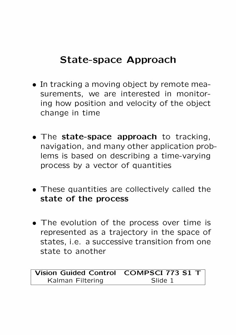
State-space Approach • In tracking a moving object by remote mea- surements, we are interested in monitor- ing how position and velocity of the object change in time • The state-space approach to tracking, navigation, and many other application prob- lems is based on describing a time-varying process by a vector of quantities • These quantities are collectively called the state of the process • The evolution of the process over time is represented as a trajectory in the space of states, i.e. a successive transition from one state to another Vision Guided Control COMPSCI 773 S1 T Kalman Filtering Slide 1
Transcript of State-space Approach - Department of Computer … · State-space Approach ... represented as a...
State-space Approach
• In tracking a moving object by remote mea-surements, we are interested in monitor-ing how position and velocity of the objectchange in time
• The state-space approach to tracking,navigation, and many other application prob-lems is based on describing a time-varyingprocess by a vector of quantities
• These quantities are collectively called thestate of the process
• The evolution of the process over time isrepresented as a trajectory in the space ofstates, i.e. a successive transition from onestate to another
Vision Guided Control COMPSCI 773 S1 TKalman Filtering Slide 1

State-space Modelling
• State: a vector of measurements for anobject describing its behaviour in time
– Example: [p, v, a] - the position, velocity, andacceleration of a moving 1D ”object” in time:v(t + ∆t) = v(t) + a(t)∆t; p(t + ∆t) = p(t) +v(t+∆t)+v(t)
2∆t = p(t) + v(t)∆t + a(t)
2∆t
• State space: the space of all possible states
• Trajectory of an object in the state space:the evolution of the object’s state in time
t 0 1 2 3 4 5a(t) 5 5 0 0 0 0v(t) 0 5 10 10 10 10p(t) 0 2.5 10 20 30 40
Vision Guided Control COMPSCI 773 S1 TKalman Filtering Slide 2
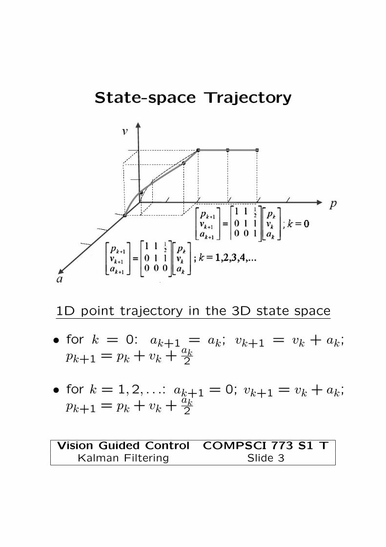
State-space Trajectory
1D point trajectory in the 3D state space
• for k = 0: ak+1 = ak; vk+1 = vk + ak;pk+1 = pk + vk + ak
2
• for k = 1,2, . . .: ak+1 = 0; vk+1 = vk + ak;pk+1 = pk + vk + ak
2
Vision Guided Control COMPSCI 773 S1 TKalman Filtering Slide 3
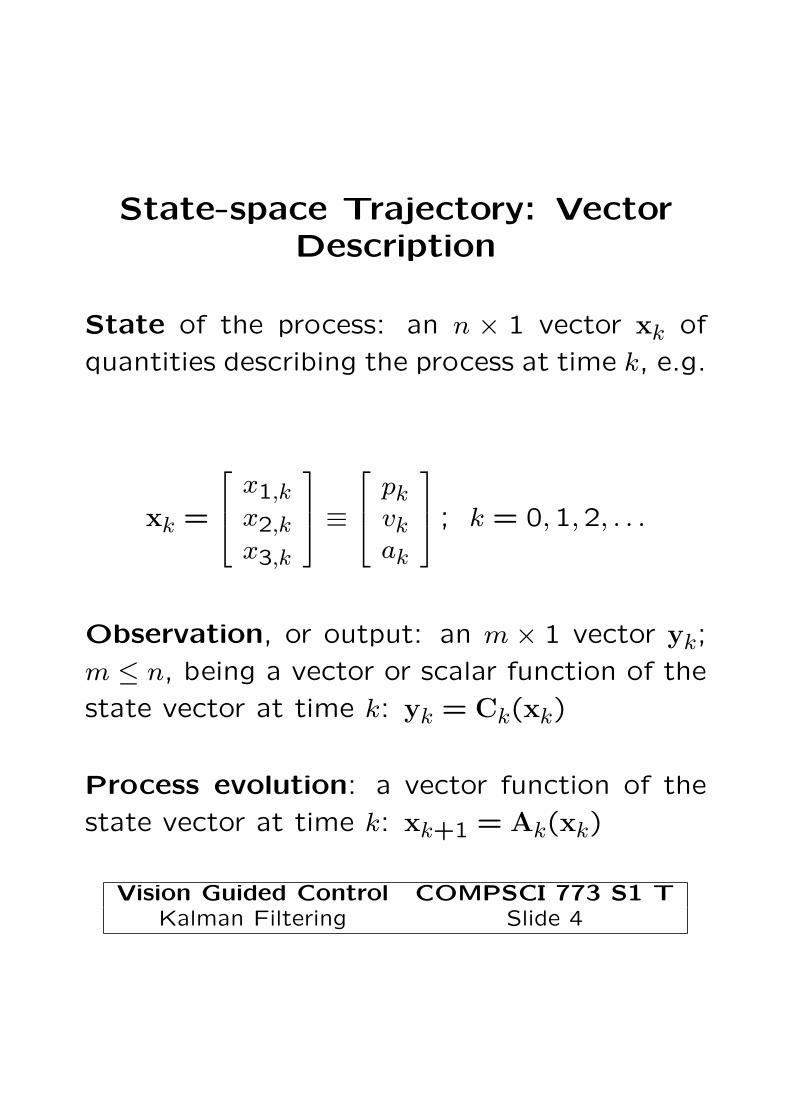
State-space Trajectory: VectorDescription
State of the process: an n × 1 vector xk of
quantities describing the process at time k, e.g.
xk =
⎡⎢⎣ x1,k
x2,kx3,k
⎤⎥⎦ ≡
⎡⎢⎣ pk
vkak
⎤⎥⎦ ; k = 0,1,2, . . .
Observation, or output: an m × 1 vector yk;
m ≤ n, being a vector or scalar function of the
state vector at time k: yk = Ck(xk)
Process evolution: a vector function of the
state vector at time k: xk+1 = Ak(xk)
Vision Guided Control COMPSCI 773 S1 TKalman Filtering Slide 4

Estimating States: General Case
• Problem: Estimate states xk from obser-vations yk; k = 0,1,2, . . .
• Basic Assumptions:
– Vector functions Ak(xk) describing theevolution of states are known for eachk but with uncertainty uk:
xk+1 = Ak(xk) + uk
– How the observation depends on the statevector is known also with measurementnoise v:
yk = Ck(xk) + vk
– Only statistical properties of the ran-dom vectors uk and vk are known
Vision Guided Control COMPSCI 773 S1 TKalman Filtering Slide 5
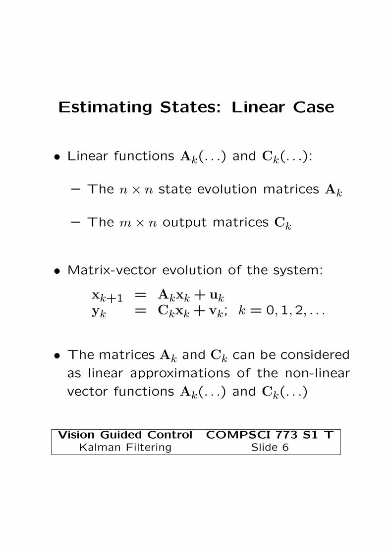
Estimating States: Linear Case
• Linear functions Ak(. . .) and Ck(. . .):
– The n × n state evolution matrices Ak
– The m × n output matrices Ck
• Matrix-vector evolution of the system:
xk+1 = Akxk + ukyk = Ckxk + vk; k = 0,1,2, . . .
• The matrices Ak and Ck can be considered
as linear approximations of the non-linear
vector functions Ak(. . .) and Ck(. . .)
Vision Guided Control COMPSCI 773 S1 TKalman Filtering Slide 6
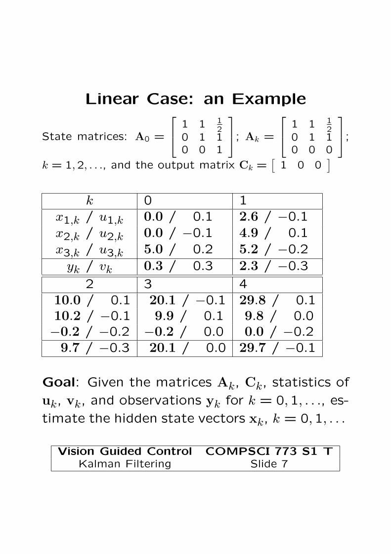
Linear Case: an Example
State matrices: A0 =
⎡⎣ 1 1 1
20 1 10 0 1
⎤⎦; Ak =
⎡⎣ 1 1 1
20 1 10 0 0
⎤⎦;
k = 1,2, . . ., and the output matrix Ck =[
1 0 0]
k 0 1x1,k / u1,k 0.0 / 0.1 2.6 / −0.1x2,k / u2,k 0.0 / −0.1 4.9 / 0.1x3,k / u3,k 5.0 / 0.2 5.2 / −0.2
yk / vk 0.3 / 0.3 2.3 / −0.3
2 3 410.0 / 0.1 20.1 / −0.1 29.8 / 0.110.2 / −0.1 9.9 / 0.1 9.8 / 0.0−0.2 / −0.2 −0.2 / 0.0 0.0 / −0.2
9.7 / −0.3 20.1 / 0.0 29.7 / −0.1
Goal: Given the matrices Ak, Ck, statistics of
uk, vk, and observations yk for k = 0,1, . . ., es-
timate the hidden state vectors xk, k = 0,1, . . .
Vision Guided Control COMPSCI 773 S1 TKalman Filtering Slide 7
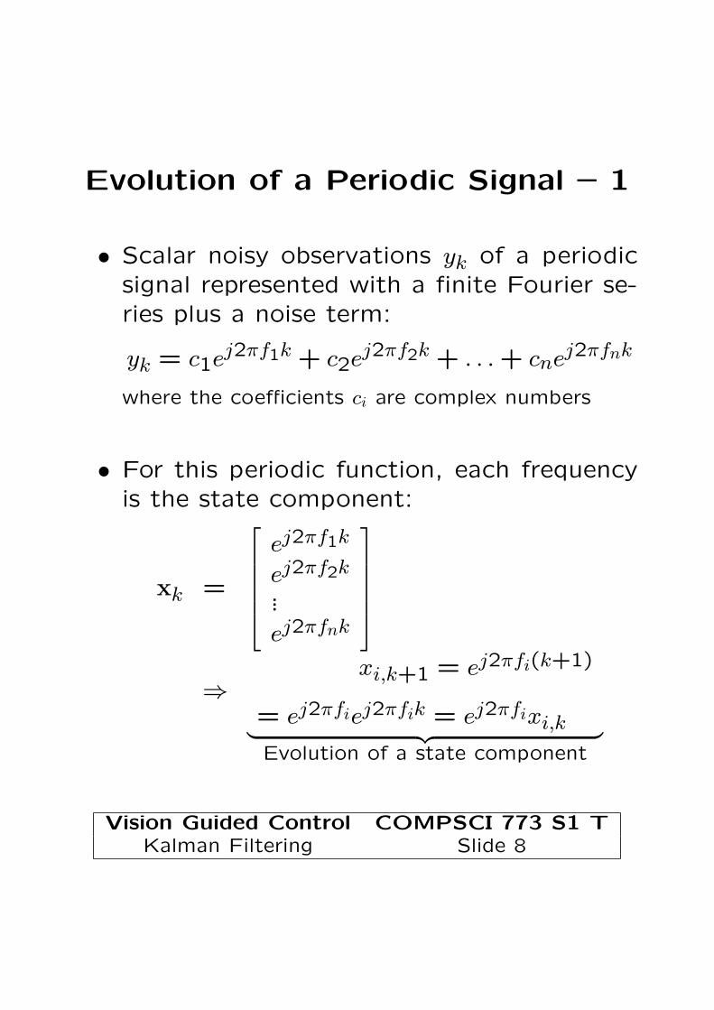
Evolution of a Periodic Signal – 1
• Scalar noisy observations yk of a periodicsignal represented with a finite Fourier se-ries plus a noise term:
yk = c1ej2πf1k + c2ej2πf2k + . . . + cnej2πfnk
where the coefficients ci are complex numbers
• For this periodic function, each frequencyis the state component:
xk =
⎡⎢⎢⎢⎢⎣
ej2πf1k
ej2πf2k
...ej2πfnk
⎤⎥⎥⎥⎥⎦
⇒xi,k+1 = ej2πfi(k+1)
= ej2πfiej2πfik = ej2πfixi,k︸ ︷︷ ︸Evolution of a state component
Vision Guided Control COMPSCI 773 S1 TKalman Filtering Slide 8
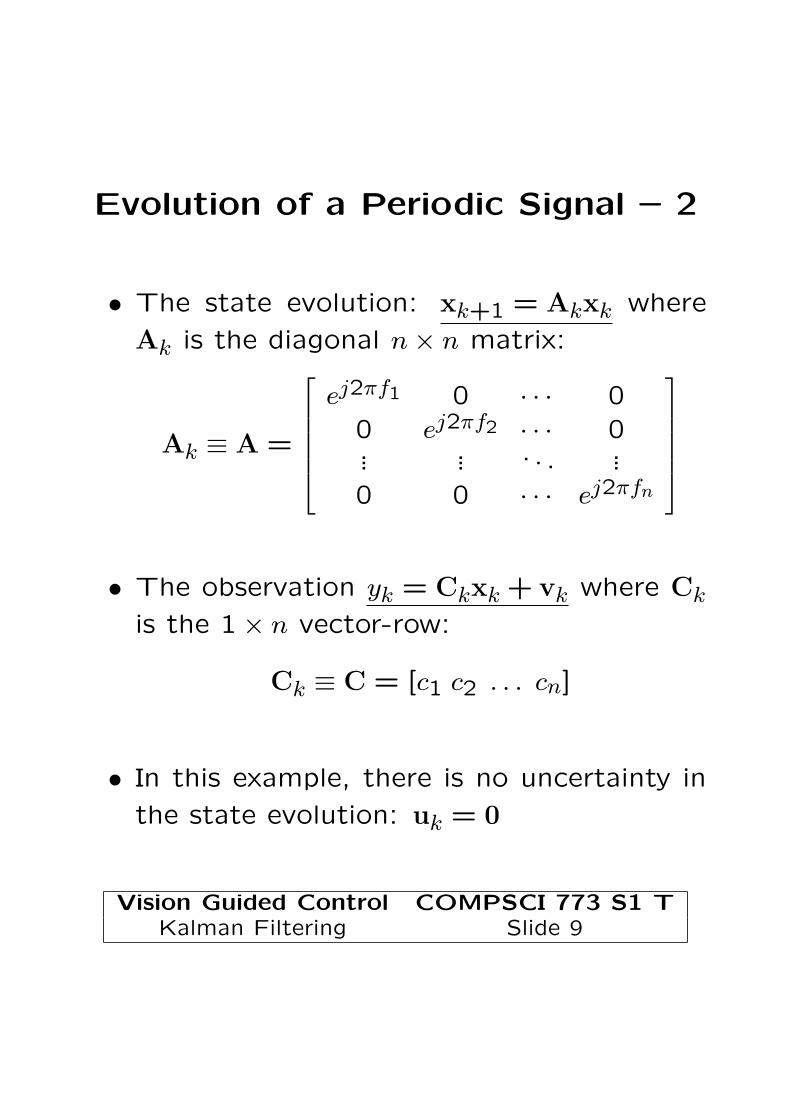
Evolution of a Periodic Signal – 2
• The state evolution: xk+1 = Akxk where
Ak is the diagonal n × n matrix:
Ak ≡ A =
⎡⎢⎢⎢⎢⎣
ej2πf1 0 · · · 00 ej2πf2 · · · 0... ... . . . ...0 0 · · · ej2πfn
⎤⎥⎥⎥⎥⎦
• The observation yk = Ckxk + vk where Ck
is the 1 × n vector-row:
Ck ≡ C = [c1 c2 . . . cn]
• In this example, there is no uncertainty in
the state evolution: uk = 0
Vision Guided Control COMPSCI 773 S1 TKalman Filtering Slide 9
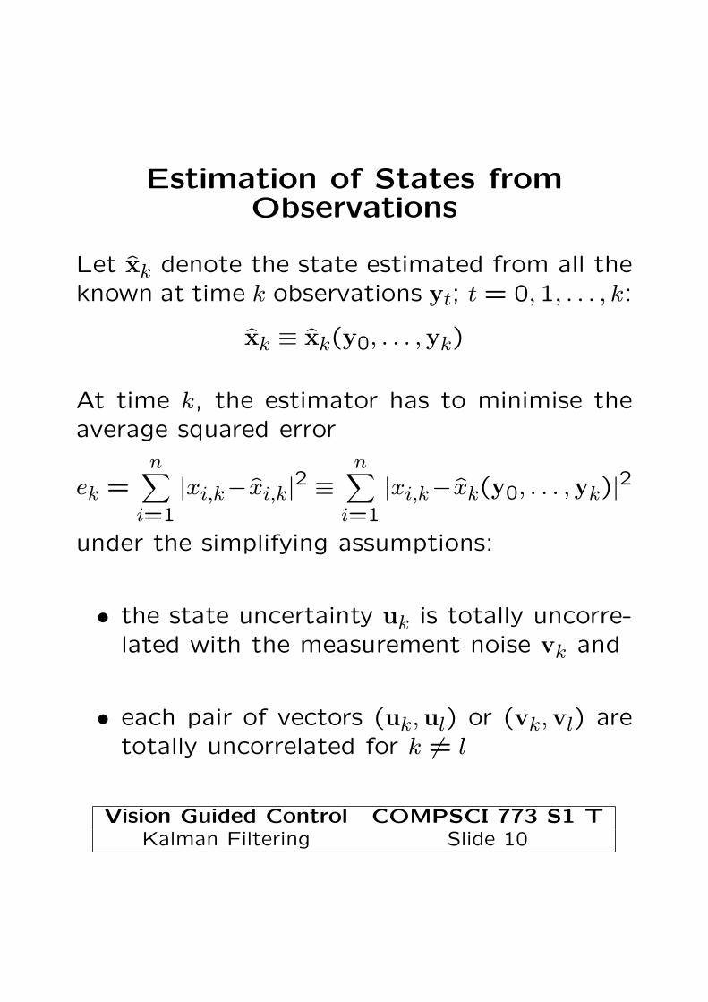
Estimation of States fromObservations
Let x̂k denote the state estimated from all theknown at time k observations yt; t = 0,1, . . . , k:
x̂k ≡ x̂k(y0, . . . ,yk)
At time k, the estimator has to minimise theaverage squared error
ek =n∑
i=1
|xi,k−x̂i,k|2 ≡n∑
i=1
|xi,k−x̂k(y0, . . . ,yk)|2
under the simplifying assumptions:
• the state uncertainty uk is totally uncorre-lated with the measurement noise vk and
• each pair of vectors (uk,ul) or (vk,vl) aretotally uncorrelated for k �= l
Vision Guided Control COMPSCI 773 S1 TKalman Filtering Slide 10
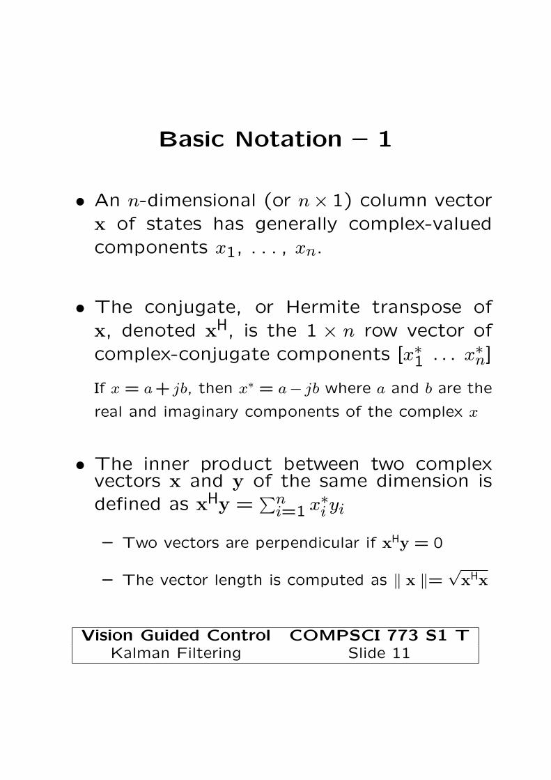
Basic Notation – 1
• An n-dimensional (or n× 1) column vectorx of states has generally complex-valuedcomponents x1, . . . , xn.
• The conjugate, or Hermite transpose ofx, denoted xH, is the 1 × n row vector ofcomplex-conjugate components [x∗1 . . . x∗n]If x = a+ jb, then x∗ = a− jb where a and b are the
real and imaginary components of the complex x
• The inner product between two complexvectors x and y of the same dimension isdefined as xHy =
∑ni=1 x∗i yi
– Two vectors are perpendicular if xHy = 0
– The vector length is computed as ‖ x ‖=√
xHx
Vision Guided Control COMPSCI 773 S1 TKalman Filtering Slide 11
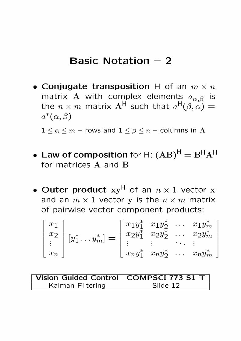
Basic Notation – 2
• Conjugate transposition H of an m × nmatrix A with complex elements aα,β isthe n × m matrix AH such that aH(β, α) =a∗(α, β)
1 ≤ α ≤ m – rows and 1 ≤ β ≤ n – columns in A
• Law of composition for H: (AB)H = BHAH
for matrices A and B
• Outer product xyH of an n × 1 vector xand an m × 1 vector y is the n × m matrixof pairwise vector component products:⎡⎢⎢⎢⎣
x1x2...xn
⎤⎥⎥⎥⎦ [
y∗1 . . . y∗m]=
⎡⎢⎢⎢⎣
x1y∗1 x1y∗2 . . . x1y∗mx2y∗1 x2y∗2 . . . x2y∗m... ... . . . ...xny∗1 xny∗2 . . . xny∗m
⎤⎥⎥⎥⎦
Vision Guided Control COMPSCI 773 S1 TKalman Filtering Slide 12

Probability Concepts – 1
• Average or expected value of a continuous
random variable: E{x} =∞∫
−∞xp(x)dx
◦ p(x): a probability density function (p.d.f.) of x
◦ E{. . .} denotes the mathematical expectation
◦ Expected vector E{x} of random variables: thevector of expected elements E{xi}; i = 1, . . . , n
◦ Expected vector sum: E{x + y} = E{x} + E{y}
◦ Expected matrix A: the matrix of expected el-ements E{A(α, β)}
• Correlation between two random variablesx and y: E{xy∗} =
∞∫−∞
xy∗p(x, y)dx
◦ p(x, y) is a joint p.d.f. of x and y
Vision Guided Control COMPSCI 773 S1 TKalman Filtering Slide 13

Probability Concepts – 2
• Correlation matrix of two vectors x and y
of random variables is the expected outer
product matrix xyH
• Entries of the correlation matrix are ex-
pected pairwise products of the scalar vec-
tor entries E{xαy∗β}
• The correlation matrix of the error xk − x̂k
is the matrix E{(xk − x̂k) (xk − x̂k)H}
• Pair of vectors x and y are uncorrelated
if E{xyH} = 0 where 0 – the matrix of ap-
propriate dimensions with zero entries
Vision Guided Control COMPSCI 773 S1 TKalman Filtering Slide 14

State / Observation StatisticsKnown by Assumption:
the n×n correlation matrix Uk for uncertaintyuk and the m × m correlation matrix Vk formeasurement noise vk for all k, l = 0, . . . , K:
E{ukuTl } =
{Uk if k = l0 otherwise
E{vkvTl } =
{Vk if k = l0 otherwise
; E{ukvTl } = 0
Components of the latter expected matrices are ex-
pected pairwise products of vector components such as
E{uk,αul,β}; α, β = 1, . . . , n, E{vk,αvl,β}; α, β = 1, . . . , m, or
E{uk,αvl,β}; α = 1, . . . , n; β = 1, . . . , m
Both the uncertainty and measurement noiseare centred: E{uk} = E{vk} = 0; k = 0,1, . . . , K
Vision Guided Control COMPSCI 773 S1 TKalman Filtering Slide 15
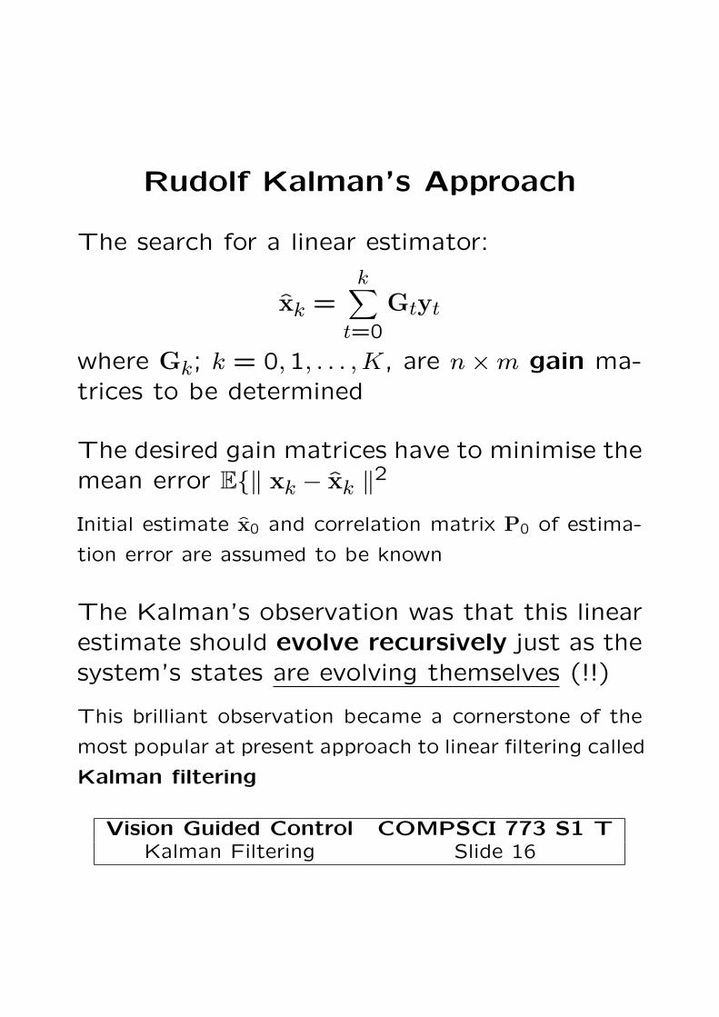
Rudolf Kalman’s Approach
The search for a linear estimator:
x̂k =k∑
t=0
Gtyt
where Gk; k = 0,1, . . . , K, are n × m gain ma-trices to be determined
The desired gain matrices have to minimise themean error E{‖ xk − x̂k ‖2Initial estimate x̂0 and correlation matrix P0 of estima-
tion error are assumed to be known
The Kalman’s observation was that this linearestimate should evolve recursively just as thesystem’s states are evolving themselves (!!)
This brilliant observation became a cornerstone of the
most popular at present approach to linear filtering called
Kalman filtering
Vision Guided Control COMPSCI 773 S1 TKalman Filtering Slide 16

Constructing a Kalman Filter – 1
Suppose an optimal linear estimate x̂k−1 basedon observations y0, y1, . . . , yk−1 is alreadyconstructed
Then x̂ik
def= Ak−1x̂k−1 is the best guess of x̂k
before making the observation yk at time k
It is the natural evolution of the estimated state vectorx̂k−1 by the linear system dynamics in Slide 6
The superscript “i” indicates this is an intermediate
estimate before constructing x̂k
yik = Ckx̂
ik is the best prediction of yk before
the actual measurement
Kalman’s proposal: the optimal solution forx̂k should be a linear combination of x̂i
k andthe difference between yk and yi
k:
x̂k = x̂ik + Gk
(yk − Ckx̂
ik
)
Vision Guided Control COMPSCI 773 S1 TKalman Filtering Slide 17

Constructing a Kalman Filter – 2
If yk = yik, then x̂k = x̂i
k = Ak−1x̂k−1, i.e. the estimate
evolves purely by what is known about the process
Optimal gain matrix Gk has to minimise the
mean error E{‖ xk − x̂k ‖2} in Slide 16:
E
{‖
(xk − x̂i
k
)− Gk
(yk − Ckx̂
ik
)‖2
}Solution: by taking and setting to zero the derivative
w.r.t. to the matrix entries
Theorem 1: Let a and b be random vectors.
Then the matrix G minimising E{‖ a − Gb ‖2}is as follows:
G = E
{abH
} (E
{bbH
})−1
providing the correlation matrix E
{bbH
}is in-
vertible.
Vision Guided Control COMPSCI 773 S1 TKalman Filtering Slide 18

Proof of Theorem 1 – (a)
Derivative of a scalar function f w.r.t. an
n × m matrix Q is defined as
∂f
∂Q=
⎡⎢⎢⎢⎢⎢⎢⎣
∂f∂Q1,1
∂f∂Q2,1
. . . ∂f∂Qn,1
∂f∂Q1,2
∂f∂Q2,2
. . . ∂f∂Qn,2
... ... . . . ...∂f
∂Q1,m
∂f∂Q2,m
. . . ∂f∂Qn,m
⎤⎥⎥⎥⎥⎥⎥⎦
For a function f = tHQs where t and s are
arbitrary n × 1 and m × 1 vectors, respectively,
the derivative is
∂
∂Q
(tHQs
)= stH
The right hand side matrix is of the dimension m × n
Each its (β, α)-entry t∗αsβ is precisely what is obtained
by differentiating the scalar function f w.r.t. the (α, β)-
entry Qα,β of Q
Vision Guided Control COMPSCI 773 S1 TKalman Filtering Slide 19

Proof of Theorem 1 – (b)
Expanding E{‖ a − Gb ‖2} gives
E
{(a − Gb)H (a − Gb)
}= E
{(aH − bHGH
)(a − Gb)
}= E
{aHa − bHGHa − aHGb + bHGHGb
}= E
{aHa
} − E{bHGHa
} − E{aHGb
}+ E
{bHGHGb
}Differentiating this with respect to the matrix G may
seen difficult because both G and GH are appearing.
It can be proven that the elements of G can be treated
as independent from the elements of GH although they
are not of course
Setting the derivative of the above expression
w.r.t. GH equal to zero produces the equation
−E
{abH
}+ GE
{bbH
}= 0
It gives the solution G = E
{abH
} (E
{bbH
})−1
Vision Guided Control COMPSCI 773 S1 TKalman Filtering Slide 20
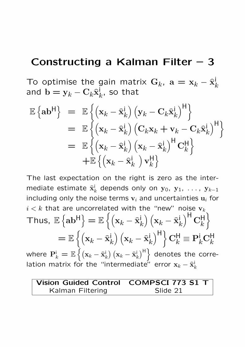
Constructing a Kalman Filter – 3
To optimise the gain matrix Gk, a = xk − x̂ik
and b = yk − Ckx̂ik, so that
E
{abH
}= E
{(xk − x̂i
k
) (yk − Ckx̂
ik
)H}
= E
{(xk − x̂i
k
) (Ckxk + vk − Ckx̂
ik
)H}
= E
{(xk − x̂i
k
) (xk − x̂i
k
)HCH
k
}+E
{(xk − x̂i
k
)vH
k
}The last expectation on the right is zero as the inter-
mediate estimate x̂ik depends only on y0, y1, . . . , yk−1
including only the noise terms vi and uncertainties ui for
i < k that are uncorrelated with the “new” noise vk
Thus, E
{abH
}= E
{(xk − x̂i
k
) (xk − x̂i
k
)HCH
k
}= E
{(xk − x̂i
k
) (xk − x̂i
k
)H}
CHk ≡ Pi
kCHk
where Pik = E
{(xk − x̂i
k
) (xk − x̂i
k
)H}
denotes the corre-
lation matrix for the “intermediate” error xk − x̂ik
Vision Guided Control COMPSCI 773 S1 TKalman Filtering Slide 21

Constructing a Kalman Filter – 4
Similar considerations result in a following sim-ple form for
E
{bbH
}= E
{(yk − Ckx̂
ik
) (yk − Ckx̂
ik
)H}
= E
{(Ckxk + vk − Ckx̂
ik
) (Ckxk + vk − Ckx̂
ik
)H}
= E
{(Ck
(xk − x̂i
k
)+ vk
) ((xk − x̂i
k
)HCH
k + vHk
)}= CkP
ikC
Hk + Vk
where Vk = E{vkvH
k
}is the measurement noise correla-
tion matrix.
By Theorem 1, the optimal gain matrix isGk = Pi
kCHk
(CkP
ikC
Hk + Vk
)−1
assuming that the inverse on the right hand side exists
The correlation matrix Pik is also computed re-
cursively starting from the matrix P0 known byassumption
Vision Guided Control COMPSCI 773 S1 TKalman Filtering Slide 22
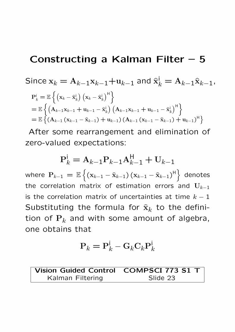
Constructing a Kalman Filter – 5
Since xk = Ak−1xk−1+uk−1 and x̂ik = Ak−1x̂k−1,
Pik = E
{(xk − x̂i
k
) (xk − x̂i
k
)H}
= E
{(Ak−1xk−1 + uk−1 − x̂i
k
) (Ak−1xk−1 + uk−1 − x̂i
k
)H}
= E
{(Ak−1 (xk−1 − x̂k−1) + uk−1) (Ak−1 (xk−1 − x̂k−1) + uk−1)
H}
After some rearrangement and elimination of
zero-valued expectations:
Pik = Ak−1Pk−1A
Hk−1 + Uk−1
where Pk−1 = E
{(xk−1 − x̂k−1) (xk−1 − x̂k−1)
H}
denotes
the correlation matrix of estimation errors and Uk−1
is the correlation matrix of uncertainties at time k − 1
Substituting the formula for x̂k to the defini-
tion of Pk and with some amount of algebra,
one obtains that
Pk = Pik − GkCkP
ik
Vision Guided Control COMPSCI 773 S1 TKalman Filtering Slide 23

How the Kalman Filter Works
Known values: yi, Vi, and Ui, Ai, and Ci for0 ≤ i ≤ k at each time k
• Initialisation k = 0: Choose or guess suit-able x̂0 and P0
• Iteration k = 1,2, . . .: Given x̂k−1 and Pk−1,compute:
1. Pik = Ak−1Pk−1A
Hk−1 + Uk−1
2. Gk = PikC
Hk
(CkP
ikC
Hk + Vk
)−1
3. x̂ik = Ak−1x̂k−1
4. x̂k = x̂ik + Gk
(yk − Ckx̂
ik
)
5. Pk = Pik − GkCkP
ik
Vision Guided Control COMPSCI 773 S1 TKalman Filtering Slide 24
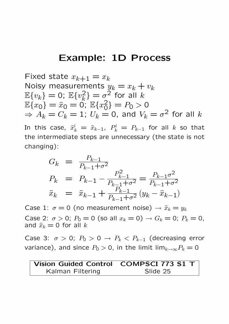
Example: 1D Process
Fixed state xk+1 = xkNoisy measurements yk = xk + vkE{vk} = 0; E{v2
k} = σ2 for all kE{x0} = x̂0 = 0; E{x2
0} = P0 > 0⇒ Ak = Ck = 1; Uk = 0, and Vk = σ2 for all k
In this case, x̂ik = x̂k−1, P i
k = Pk−1 for all k so that
the intermediate steps are unnecessary (the state is not
changing):
Gk =Pk−1
Pk−1+σ2
Pk = Pk−1 − P2k−1
Pk−1+σ2 =Pk−1σ2
Pk−1+σ2
x̂k = x̂k−1 +Pk−1
Pk−1+σ2
(yk − x̂k−1
)Case 1: σ = 0 (no measurement noise) → x̂k = yk
Case 2: σ > 0; P0 = 0 (so all xk = 0) → Gk = 0; Pk = 0,and x̂k = 0 for all k
Case 3: σ > 0; P0 > 0 → Pk < Pk−1 (decreasing error
variance), and since P0 > 0, in the limit limk→∞Pk = 0
Vision Guided Control COMPSCI 773 S1 TKalman Filtering Slide 25