State of the Art in Forecasting of Wind and Solar Power...

State-of-the-art in Forecasting ofWind and Solar Power Generation

Henrik Madsen1, Pierre Pinson, Peder Bacher1,

Jan Kloppenborg1, Julija Tastu1, Emil Banning Iversen1

[email protected]

(1) Department of Applied Mathematics and Computer Science

DTU, DK-2800 Lyngby

www.henrikmadsen.org

Wind and Solar Power Forecasting, ESI 101 Course, July 2014 – p. 1

www.henrikmadsen.org

Outline

I shall focus on Wind - and briefly mention Solar and Load:

Status in Denmark

Wind power point forecasting

Use of several providers of MET forecasts

Uncertainty and confidence intervals

Scenario forecasting

Space-time scenario forecasting

Use of stochastic differential equations

Examples on the use of probabilistic forecasts

Optimal bidding for a wind farm owner

Solar power forecasting

Lessons learned in DenmarkWind and Solar Power Forecasting, ESI 101 Course, July 2014 – p. 2

Some Wind Power Statistics for Denmark


Power Grid. A snap-shot from 14. February


Wind Power Forecasting - History

Our methods for probabilistic wind power forecasting have been implemented in theAnemos Wind Power Prediction System, Australian Wind Energy Forecasting Systems(AWEFS) andWPPT

The methods have been continuously developed since 1993 - incollaboration withEnerginet.dk,Dong Energy,Vattenfall,Risø – DTU Wind,The ANEMOS projects partners/consortium (since 2002),Overspeed GmbH (Anemos: www.overspeed.de/gb/produkte/windpower.html)ENFOR (WPPT: www.enfor.dk)

Used operationally for predicting wind power in Denmark since 1996.

Now used by all major players in Denmark (Energinet.dk, DONG, Vattenfall, ..)

Anemos/WPPT is now used eg in Europe, Australia, and North America.

Often used as forecast engine embedded in other systems.


Prediction Performance

A typical (power curve only!) performance measure. 13 largeparks. Installed power: 1064MW. Period: August 2008 - March 2010. MET input is in all casesECMWF. Criterion used:RMSE (notice:Power Curve model only)

Forecast horizon (hours)

Nor

mal

ized

pow

er

0.00

0.05

0.10

0.15

0 12 24 36 48

Nominal power: 1064 MW

RMSE

WPPT−PCSimple modelCommercial model 1Commercial model 2


Prediction of wind power

In areas with high penetration of wind power such as the Western part of Denmark and theNorthern part of Germany and Spain, reliable wind power predictions are needed in order toensure safe and economic operation of the power system.

Accurate wind power predictions are needed with different prediction horizons in order toensure

(up to a few hours) efficient and safe use of regulation power (spinning reserve) andthe transmission system,

(12 to 36 hours) efficient trading on the Nordic power exchange, NordPool,

(days) optimal operation of eg. large CHP plants.

Predictions of wind power are needed both for the total supply area as well as on a regionalscale and for single wind farms.

For some grids/in some situations the focus is on methods forramp forecasting, in someother cases the focus in on reliable probabilistic forecasting.


Uncertainty and adaptivity

Errors in MET forecasts will end up in errors in wind power forecasts, but other factors leadto a need for adaptation which however leads to some uncertainties.

The total system consisting of wind farms measured online, wind turbines not measuredonline and meteorological forecasts will inevitably change over time as:

the population of wind turbines changes,

changes in unmodelled or insufficiently modelled characteristics (importantexamples: roughness and dirty blades),

changes in the NWP models.

A wind power prediction system must be able to handle these time-variations in model andsystem. An adequate forecasting system may useadaptive and recursive model estimationto handle these issues.

We started (some 20 years ago) assuming Gaussianity; but this is a very serious (wrong)assumption !

Following the initial installation the software tool will automatically calibrate the models tothe actual situation.


The power curve model

The wind turbine “power curve” model,ptur = f(wtur) is extended to a wind farmmodel, pwf = f(wwf , θwf ), by introducingwind direction dependency. By introducing arepresentative area wind speed and direction itcan be further extended to cover all turbines inan entire region,par = f(w̄ar, θ̄ar).

The power curve model is defined as:

p̂t+k|t = f( w̄t+k|t, θ̄t+k|t, k )

wherew̄t+k|t is forecasted wind speed, andθ̄t+k|t is forecasted wind direction.

The characteristics of the NWP change withthe prediction horizon.

k

Wind speedWind direction

P

k


P

k


P

k


P

HO - Estimated power curve

Plots of the estimated power curve forthe Hollandsbjerg wind farm.


The dynamical prediction model

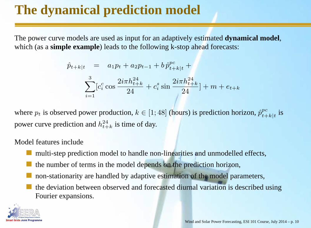
The power curve models are used as input for an adaptively estimateddynamical model,which (as asimple example) leads to the following k-stop ahead forecasts:

p̂t+k|t = a1pt + a2pt−1 + b p̂pc

t+k|t +

3∑

i=1

[cci cos2iπh24

t+k

24+ c

si sin

2iπh24t+k

24] +m+ et+k

wherept is observed power production,k ∈ [1; 48] (hours) is prediction horizon,̂ppct+k|t is

power curve prediction andh24t+k is time of day.

Model features include

multi-step prediction model to handle non-linearities andunmodelled effects,

the number of terms in the model depends on the prediction horizon,

non-stationarity are handled by adaptive estimation of themodel parameters,

the deviation between observed and forecasted diurnal variation is described usingFourier expansions.


A model for upscaling

The dynamic upscaling model for a region is defined as:

p̂reg

t+k|t = f( w̄art+k|t, θ̄

art+k|t, k ) p̂loct+k|t

wherep̂loct+k|t is a local (dynamic) power prediction within the region,w̄ar

t+k|t is forecasted regional wind speed, and

θ̄art+k|t is forecasted regional wind direction.

The characteristics of the NWP andp̂loc change with the prediction horizon. Hence thedependendency of prediction horizonk in the model.


Configuration Example

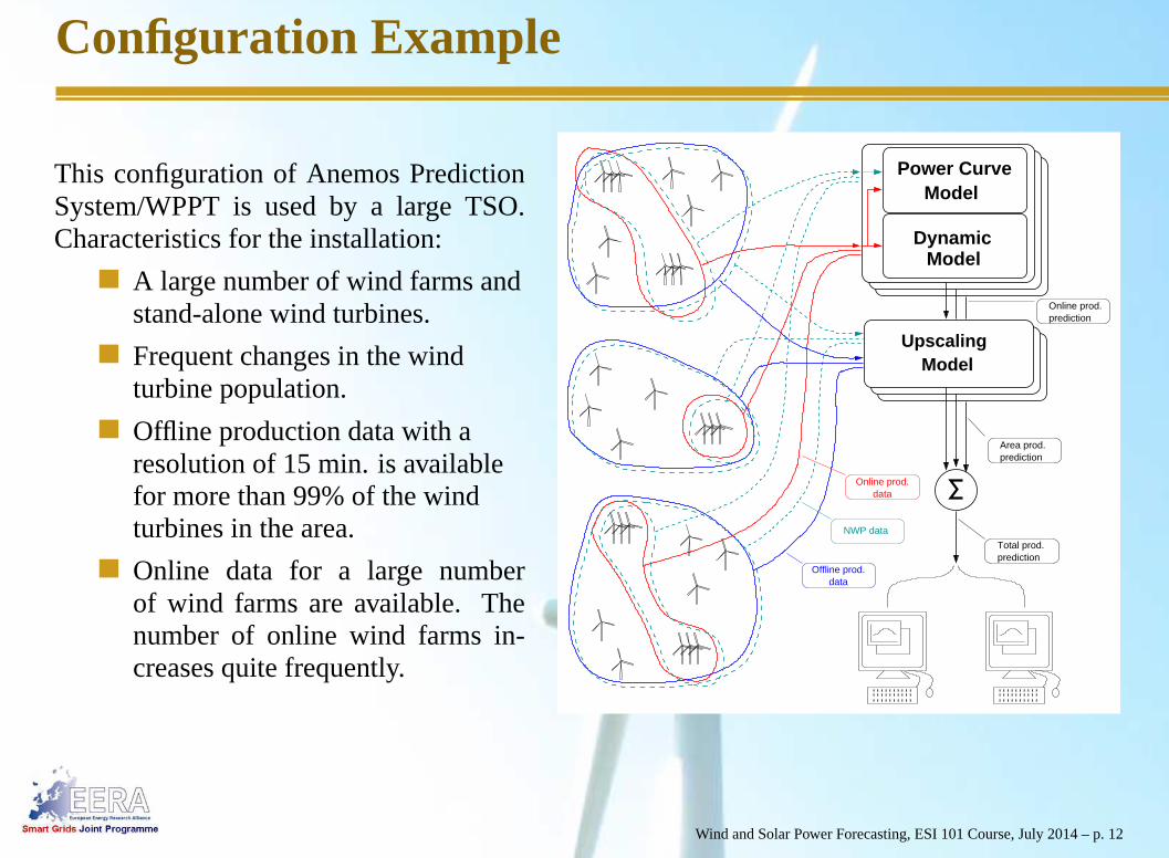
This configuration of Anemos PredictionSystem/WPPT is used by a large TSO.Characteristics for the installation:

A large number of wind farms andstand-alone wind turbines.

Frequent changes in the windturbine population.

Offline production data with aresolution of 15 min. is availablefor more than 99% of the windturbines in the area.

Online data for a large numberof wind farms are available. Thenumber of online wind farms in-creases quite frequently.

ModelUpscaling

predictionTotal prod.

Dynamic

Power CurveModel

Model

Offline prod.data

predictionArea prod.

NWP data

Online prod.data

predictionOnline prod.


Fluctuations of offshore wind power

Fluctuations at large offshore wind farms have a significantimpact on the control andmanagement strategies of their power output

Focus is given to the minute scale. Thus, the effects relatedto the turbulent nature ofthe wind are smoothed out

When looking at time-series of power production at Horns Rev(160MW/209MW)and Nysted (165 MW), one observes successive periods with fluctuations of largerand smaller magnitude

We aim at building models

based on historical wind powermeasures only...... but able to reproduce thisobserved behavior

this calls forregime-switchingmodels


Results - Horns Rev

The evaluation set is

divided in 19 different

periods of different

lengths and

characteristics

MSAR models

generally outperform

the others

In the RADAR@sea

project the regime shift

is linked to convective

rain events – which are

detected by a weather

radar.

2 4 6 8 10 12 14 16 1810

15

20

25

30

Test data set

RM

SE

[kW

]

1 minute Horns Rev SETARMSARSTARARMA

2 4 6 8 10 12 14 16 1820

40

60

80

100

Test data set

RM

SE

[kW

]

5 minute Horns RevSETARMSARSTARARMA

2 4 6 8 10 12 14 16 180

50

100

150

Test data set

RM

SE

[kW

]

10 minute Horns RevSETARMSARSTARARMA


Spatio-temporal forecasting

Predictive improvement (measured inRMSE) of forecasts errors by adding thespatio-temperal module in WPPT.

23 months (2006-2007)

15 onshore groups

Focus here on 1-hour forecast only

Larger improvements for eastern partof the region

Needed for reliable ramp forecasting.

The EU project NORSEWinD willextend the region


Combined forecasting

A number of power forecasts areweighted together to form a newimproved power forecast.

These could come from parallelconfigurations of WPPT using NWPinputs fromdifferent METproviders or they could come fromother power prediction providers.

In addition to the improved perfor-mance also the robustness of the sys-tem is increased.

Met Office

DWD

DMI

WPPT

WPPT

WPPT

Comb Final

The example show results achieved for theTunø Knob wind farms using combinationsof up to 3 power forecasts.

Hours since 00Z

RM

S (

MW

)

5 10 15 20

5500

6000

6500

7000

7500

hir02.locmm5.24.loc

C.allC.hir02.loc.AND.mm5.24.loc

Typically an improvement on 10-15 pctin accuracy of the point prediction isseen by including more than one METprovider. Two or more MET providersimply information about uncertainty


Uncertainty estimation

In many applications it is crucial that a pre-diction tool delivers reliable estimates (prob-abilistc forecasts) of the expected uncertaintyof the wind power prediction.

We consider the following methods for esti-mating the uncertainty of the forecasted windpower production:

Ensemble based - but corrected -quantiles.

Quantile regression.

Stochastic differential equations.

The plots show raw (top) and corrected (bot-tom) uncertainty intervales based on ECMEFensembles for Tunø Knob (offshore park),29/6, 8/10, 10/10 (2003). Shown are the25%, 50%, 75%, quantiles.

Tunø Knob: Nord Pool horizons (init. 29/06/2003 12:00 (GMT), first 12h not in plan)

kW

12:00 18:00 0:00 6:00 12:00 18:00 0:00Jun 30 2003 Jul 1 2003 Jul 2 2003

020

0040

00


kW

12:00 18:00 0:00 6:00 12:00 18:00 0:00Oct 9 2003 Oct 10 2003 Oct 11 2003

020

0040

00


kW

12:00 18:00 0:00 6:00 12:00 18:00 0:00Oct 11 2003 Oct 12 2003 Oct 13 2003

020

0040

00


kW

12:00 18:00 0:00 6:00 12:00 18:00 0:00Jun 30 2003 Jul 1 2003 Jul 2 2003

020

0040

00


kW

12:00 18:00 0:00 6:00 12:00 18:00 0:00Oct 9 2003 Oct 10 2003 Oct 11 2003

020

0040

00


kW

12:00 18:00 0:00 6:00 12:00 18:00 0:00Oct 11 2003 Oct 12 2003 Oct 13 2003

020

0040

00


Quantile regression

A (additive) model for each quantile:

Q(τ) = α(τ) + f1(x1; τ) + f2(x2; τ) + . . .+ fp(xp; τ)

Q(τ) Quantile offorecast error from anexisting system.

xj Variables which influence the quantiles, e.g. the wind direction.

α(τ) Intercept to be estimated from data.

fj(·; τ) Functions to be estimated from data.

Notes on quantile regression:

Parameter estimates found by minimizing a dedicated function of the

prediction errors.

The variation of the uncertainty is (partly) explained by the independent

variables.Wind and Solar Power Forecasting, ESI 101 Course, July 2014 – p. 18

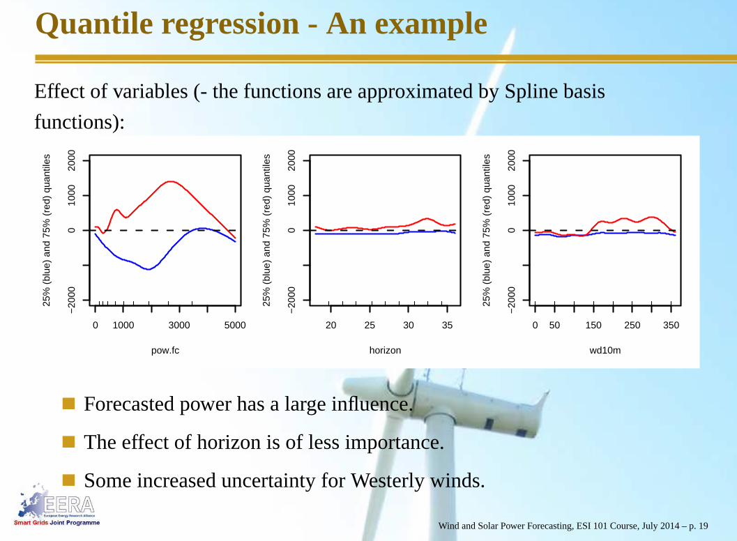
Quantile regression - An example

Effect of variables (- the functions are approximated by Spline basis

functions):

0 1000 3000 5000

−20

000

1000

2000

pow.fc

25%

(bl

ue)

and

75%

(re

d) q

uant

iles

20 25 30 35

−20

000

1000

2000

horizon

25%

(bl

ue)

and

75%

(re

d) q

uant

iles

0 50 150 250 350

−20

000

1000

2000

wd10m

25%

(bl

ue)

and

75%

(re

d) q

uant

iles

Forecasted power has a large influence.

The effect of horizon is of less importance.

Some increased uncertainty for Westerly winds.


Example: Probabilistic forecasts

5 10 15 20 25 30 35 40 450

10

20

30

40

50

60

70

80

90

100

look−ahead time [hours]

pow

er [%

of P

n]

90%80%70%60%50%40%30%20%10%pred.meas.

Notice how the confidence intervals varies ...

But the correlation in forecasts errors is not described so far.


Correlation structure of forecast errors

It is important to model theinterdependence structureof the prediction errors.

An example of interdependence covariance matrix:

5 10 15 20 25 30 35 40

5

10

15

20

25

30

35

40

horizon [h]

horiz

on[h

]

−0.2

0

0.2

0.4

0.6

0.8

1


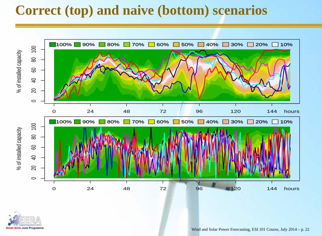
Correct (top) and naive (bottom) scenarios%

of in

stalle

d ca

pacit

y

0 24 48 72 96 120 144

020

4060

8010

0

hours

100% 90% 80% 70% 60% 50% 40% 30% 20% 10%100% 90% 80% 70% 60% 50% 40% 30% 20% 10%

% o

f insta

lled

capa

city

0 24 48 72 96 120 144

020

4060

8010

0

hours

100% 90% 80% 70% 60% 50% 40% 30% 20% 10%100% 90% 80% 70% 60% 50% 40% 30% 20% 10%


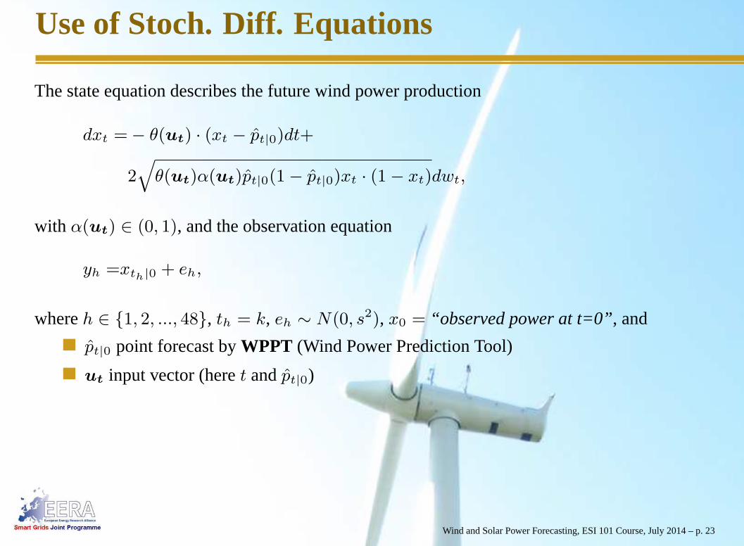
Use of Stoch. Diff. Equations

The state equation describes the future wind power production

dxt =− θ(ut) · (xt − p̂t|0)dt+

2√

θ(ut)α(ut)p̂t|0(1− p̂t|0)xt · (1− xt)dwt,

with α(ut) ∈ (0, 1), and the observation equation

yh =xth|0 + eh,

whereh ∈ {1, 2, ..., 48}, th = k, eh ∼ N(0, s2), x0 = “observed power at t=0”, and

p̂t|0 point forecast byWPPT (Wind Power Prediction Tool)

ut input vector (heret andp̂t|0)


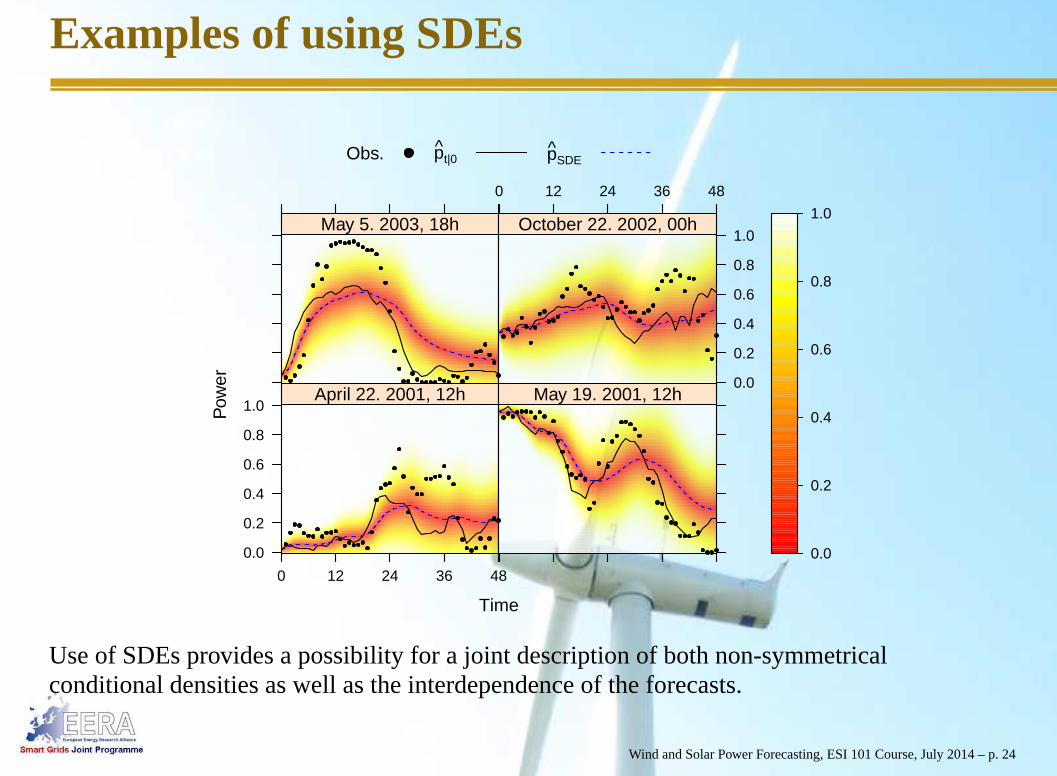
Examples of using SDEs

Time

Pow

er

0.0

0.2

0.4

0.6

0.8

1.0

0 12 24 36 48

April 22. 2001, 12h May 19. 2001, 12h

May 5. 2003, 18h

0 12 24 36 48

0.0

0.2

0.4

0.6

0.8

1.0October 22. 2002, 00h

0.0

0.2

0.4

0.6

0.8

1.0

Obs. p̂t|0 p̂SDE

Use of SDEs provides a possibility for a joint description ofboth non-symmetricalconditional densities as well as the interdependence of theforecasts.


SDE approach – Correlation structures

Time

Tim

e

12

24

36

48

12 24 36 48

April 22. 2001, 12h May 19. 2001, 12h

May 5. 2003, 18h

12 24 36 48

12

24

36

48October 22. 2002, 00h

0.0

0.2

0.4

0.6

0.8

1.0

Use of SDEs provides a possibility to model eg. time varying and wind power dependentcorrelation structures.SDEs provide a perfect framework forcombined wind and solar power forecasting.Today bothAnemos Wind Power Prediction SystemandWPPT provide operationsforecasts of both wind and solar power production (used eg. all over Australia)


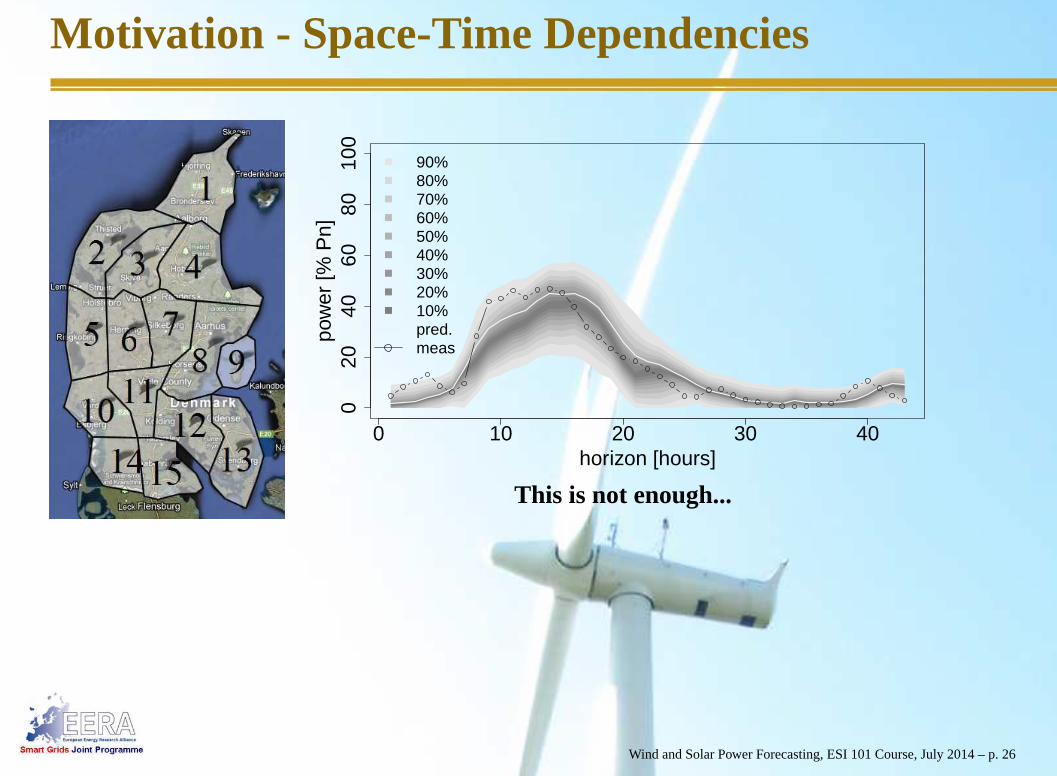
Motivation - Space-Time Dependencies

0 10 20 30 40

020

4060

8010

0

horizon [hours]

pow

er [%

Pn]

90% 80% 70% 60% 50% 40% 30% 20% 10% pred.meas

This is not enough...


Space-Time Correlations


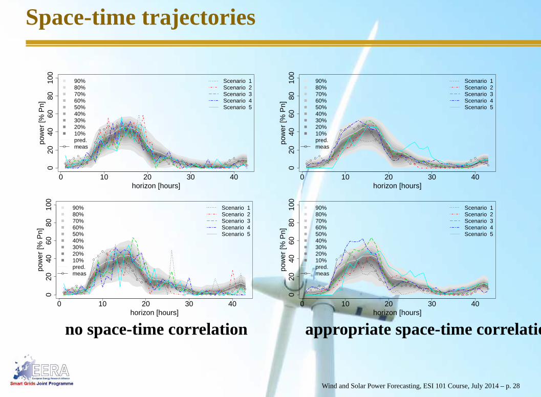
Space-time trajectories

0 10 20 30 40

020

4060

8010

0

horizon [hours]

pow

er [%

Pn]

90% 80% 70% 60% 50% 40% 30% 20% 10% pred.meas

Scenario 1Scenario 2Scenario 3Scenario 4Scenario 5

0 10 20 30 40

020

4060

8010

0

horizon [hours]

pow

er [%

Pn]

90% 80% 70% 60% 50% 40% 30% 20% 10% pred.meas


0 10 20 30 40

020

4060

8010

0

horizon [hours]

pow

er [%

Pn]

90% 80% 70% 60% 50% 40% 30% 20% 10% pred.meas


0 10 20 30 40

020

4060

8010

0

horizon [hours]

pow

er [%

Pn]

90% 80% 70% 60% 50% 40% 30% 20% 10% pred.meas


no space-time correlation appropriate space-time correlation


Type of forecasts required

Point forecasts (normal forecasts); a single value for each time point in the future.Sometimes with simple error bands.

Probabilistic or quantile forecasts; the full conditional distribution for each timepoint in the future.

Scenarios; probabilistic correct scenarios of the future wind power production.


Value of knowing the uncertainties

Case study: A 15 MW wind farm in the Dutch electricity market,prices andmeasurements from the entire year 2002.

From a phd thesis by Pierre Pinson (2006).

The costs are due to the imbalance penalties on the regulation market.

Value of an advanced method for point forecasting:The regulation costs arediminished by nearly 38 pct.compared to the costs of using the persistanceforecasts.

Added value of reliable uncertainties:A further decrease of regulation costs – up to39 pct.


Wind power – asymmetrical penalties

The revenue from trading a specific hour on NordPool can be expressed as

PS × Bid +

{

PD × (Actual− Bid) if Actual > BidPU × (Actual− Bid) if Actual < Bid

PS is the spot price andPD/PU is the down/up reg. price.

The bid maximising the expected revenue is the followingquantile

E[PS ]− E[PD]

E[PU ]− E[PD]

in the conditional distribution of the future wind power production.


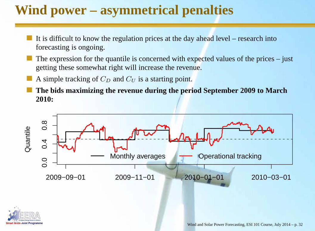
Wind power – asymmetrical penalties

It is difficult to know the regulation prices at the day ahead level – research intoforecasting is ongoing.

The expression for the quantile is concerned with expected values of the prices – justgetting these somewhat right will increase the revenue.

A simple tracking ofCD andCU is a starting point.

The bids maximizing the revenue during the period September 2009 to March2010:

Qua

ntile

0.0

0.4

0.8

2009−09−01 2009−11−01 2010−01−01 2010−03−01

Monthly averages Operational tracking


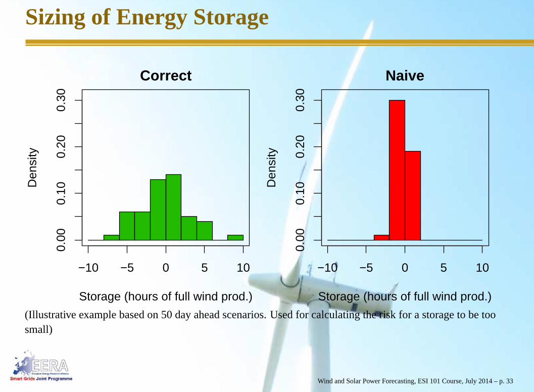
Sizing of Energy Storage

Correct

Storage (hours of full wind prod.)

Den

sity

−10 −5 0 5 10

0.00

0.10

0.20

0.30

Naive

Storage (hours of full wind prod.)

Den

sity

−10 −5 0 5 10

0.00

0.10

0.20

0.30

(Illustrative example based on 50 day ahead scenarios. Usedfor calculating the risk for a storage to be toosmall)


Wind and EU cross-border power flows

Map of thenonlinear impact andsensitivity of EU power flowsto predicted wind power penetration in Germany... here if within10-15% of installed capacity


Solar Power Forecasting

Same principles as for wind power ....

Developed for grid connected PV-systems mainly installed on rooftops

Average of output from 21 PV systems in small village (Brædstrup) in DK


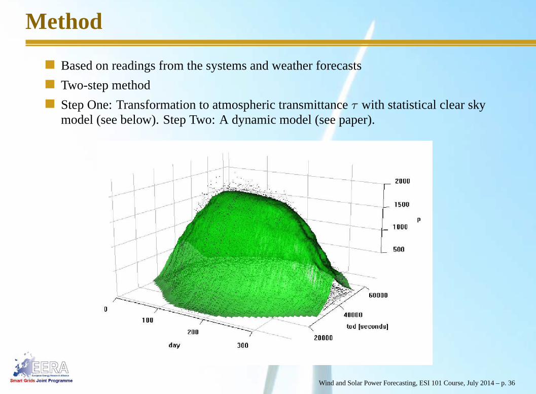
Method

Based on readings from the systems and weather forecasts

Two-step method

Step One: Transformation to atmospheric transmittanceτ with statistical clear skymodel (see below). Step Two: A dynamic model (see paper).


Example of hourly forecasts


Software Modules for Wind Power Forecasting

Point prediction module

Probabilistic (quantile) forecasting module

Scenario generation module

Spatio-temporal forecasting module

Space-time scenario generation module

Even-based prediction module (eg. cut-off prob.)

Ramp prediction module

Same modules are available for solar Power Forecasting


VG-Integration: Lessons Learned in Denmark

(> 5 pct wind): Tools for Wind/Solar Power forecasting are important

(> 10 pct wind): Tools for reliable probabilistic forecasting are needed

(> 15 pct wind): Consider Energy Systems Integration (not Power alone)

(> 20 pct wind): Consider Methods for Demand Side Management

(> 25 pct wind): New methods for finding the optimal spinning reserve are needed(based on prob. forecasting of wind/solar power production)

Joint forecasts of wind, solar, load and prices are essential

Limited need - or no need - for classical storage solutions

Huge need for virtual storage solutions

Intelligent interaction between power, gas, DH and biomassvery important

ICT and use of data, adaptivity, intelligence, and stochastic modelling is veryimportant

The largest national strategic research project:Centre for IT-Intelligent Energy Systems inCities - CITIES have been launched 1. January 2014. International expertice from NREL(US), UCD/ERC (Ireland), AIT (Austria) becomes important.


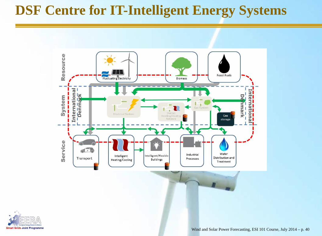
DSF Centre for IT-Intelligent Energy Systems


Wind Power Forecasting - Lessons Learned

The forecasting models must beadaptive (in order to taken changes of dust onblades, changes roughness, etc., into account).

Reliable estimates of theforecast accuracyis very important (check the reliability byeg. reliability diagrams).

Reliable probabilistic forecasts are important to gain thefull economical value.

Usemore than a single MET provider for delivering the input to the prediction tool– this improves the accuracy of wind power forecasts with 10-15 pct.

Estimates of thecorrelation in forecasts errors important.

Forecasts of ’cross dependencies’ between load, prices, wind and solar power areimportant.

Probabilistic forecasts are very important for asymmetric cost functions.

Probabilistic forecasts can provideanswersfor questions likeWhat is the probability that a given storage is large enough for the next 5 hours?What is the probability of an increase in wind power production of more that 50pct of installed power over the next two hours?What is the probability of a down-regulation due to wind power on more than xGW within the next 4 hours.

The same conclusions hold for our tools foreg. solar power forecasting.Wind and Solar Power Forecasting, ESI 101 Course, July 2014 – p. 41

Some Forecasting Tools from DTU

Forecasting and optimisation tools enabling the integration of a large share ofrenewables:

Electricity load forecasts: LoadForWind power production: WPPTSolar power production: SolarForGas load: GasforHeat load: PRESSOptimal operation of CHP systems: PRESSPrice forecasts: PriceForLately: Wave power forecasts


Some references

H. Madsen:Time Series Analysis, Chapman and Hall, 392 pp, 2008.

J.M. Morales, A.J. Conejo, H. Madsen, P. Pinson, M. Zugno:Integrating Renewables in Electricity

Markes, Springer, 430 pp., 2013.

G. Giebel, R. Brownsword, G. Kariniotakis, M. Denhard, C. Draxl: The state-of-the-art in

short-term prediction of wind power, ANEMOS plus report, 2011.

P. Meibom, K. Hilger, H. Madsen, D. Vinther:Energy Comes together in Denmark, IEEE Power

and Energy Magazin, Vol. 11, pp. 46-55, 2013.

T.S. Nielsen, A. Joensen, H. Madsen, L. Landberg, G. Giebel:A New Reference for Predicting

Wind Power, Wind Energy, Vol. 1, pp. 29-34, 1999.

H.Aa. Nielsen, H. Madsen:A generalization of some classical time series tools, Computational

Statistics and Data Analysis, Vol. 37, pp. 13-31, 2001.

H. Madsen, P. Pinson, G. Kariniotakis, H.Aa. Nielsen, T.S. Nilsen: Standardizing the performance

evaluation of short-term wind prediction models, Wind Engineering, Vol. 29, pp. 475-489, 2005.

H.A. Nielsen, T.S. Nielsen, H. Madsen, S.I. Pindado, M. Jesus, M. Ignacio:Optimal Combination

of Wind Power Forecasts, Wind Energy, Vol. 10, pp. 471-482, 2007.

A. Costa, A. Crespo, J. Navarro, G. Lizcano, H. Madsen, F. Feitosa,A review on the young history

of the wind power short-term prediction, Renew. Sustain. Energy Rev., Vol. 12, pp. 1725-1744,

2008.


Some references (Cont.)

J.K. Møller, H. Madsen, H.Aa. Nielsen:Time Adaptive Quantile Regression, Computational

Statistics and Data Analysis, Vol. 52, pp. 1292-1303, 2008.

P. Bacher, H. Madsen, H.Aa. Nielsen:Online Short-term Solar Power Forecasting, Solar Energy,

Vol. 83(10), pp. 1772-1783, 2009.

P. Pinson, H. Madsen:Ensemble-based probabilistic forecasting at Horns Rev. Wind Energy, Vol.

12(2), pp. 137-155 (special issue on Offshore Wind Energy),2009.

P. Pinson, H. Madsen:Adaptive modeling and forecasting of wind power fluctuations with

Markov-switching autoregressive models. Journal of Forecasting, 2010.

C.L. Vincent, G. Giebel, P. Pinson, H. Madsen:Resolving non-stationary spectral signals in wind

speed time-series using the Hilbert-Huang transform. Journal of Applied Meteorology and

Climatology, Vol. 49(2), pp. 253-267, 2010.

P. Pinson, P. McSharry, H. Madsen.Reliability diagrams for nonparametric density forecastsof

continuous variables: accounting for serial correlation. Quarterly Journal of the Royal

Meteorological Society, Vol. 136(646), pp. 77-90, 2010.

C. Gallego, P. Pinson, H. Madsen, A. Costa, A. Cuerva (2011).Influence of local wind speed and

direction on wind power dynamics - Application to offshore very short-term forecasting. Applied

Energy, in press


Some references (Cont.)

C.L. Vincent, P. Pinson, G. Giebel (2011).Wind fluctuations over the North Sea. International

Journal of Climatology, available online

J. Tastu, P. Pinson, E. Kotwa, H.Aa. Nielsen, H. Madsen (2011). Spatio-temporal analysis and

modeling of wind power forecast errors. Wind Energy 14(1), pp. 43-60

F. Thordarson, H.Aa. Nielsen, H. Madsen, P. Pinson (2010).Conditional weighted combination of

wind power forecasts. Wind Energy 13(8), pp. 751-763

P. Pinson, H.Aa. Nielsen, H. Madsen, G. Kariniotakis (2009). Skill forecasting from ensemble

predictions of wind power. Applied Energy 86(7-8), pp. 1326-1334.

P. Pinson, H.Aa. Nielsen, J.K. Moeller, H. Madsen, G. Kariniotakis (2007).Nonparametric

probabilistic forecasts of wind power: required properties and evaluation. Wind Energy 10(6), pp.

497-516.

T. Jónsson, P. Pinson (2010).On the market impact of wind energy forecasts. Energy Economics,

Vol. 32(2), pp. 313-320.

T. Jónsson, M. Zugno, H. Madsen, P. Pinson (2010).On the Market Impact of Wind Power

(Forecasts) - An Overview of the Effects of Large-scale Integration of Wind Power on the Electricity

Market. IAEE International Conference, Rio de Janeiro, Brazil.


State of the Art in Forecasting of Wind and Solar Power...

Documents

Transcript of State of the Art in Forecasting of Wind and Solar Power...