ADA Notice For individuals with sensory disabilities, this document is available in alternate formats. For information call (916) 654-6410 or TDD (916) 654-3880 or write Records and Forms Management, 1120 N Street, MS-89, Sacramento, CA 95814.

STATE OF CALIFORNIA • DEPARTMENT OF TRANSPORTATION TECHNICAL REPORT DOCUMENTATION PAGE TR0003 (REV 10/98)

1. REPORT NUMBER

CA17-2980 2. GOVERNMENT ASSOCIATION NUMBER 3. RECIPIENT'S CATALOG NUMBER

4. TITLE AND SUBTITLE

Biking in Fresh Air: Consideration of Exposure to Traffic-Related Air Pollution in Bicycle Route Planning

5. REPORT DATE

March 2017 6. PERFORMING ORGANIZATION CODE

7. AUTHOR

Kanok Boriboonsomsin, Jill Luo

8. PERFORMING ORGANIZATION REPORT NO.

DTRT13-G-UTC29

9. PERFORMING ORGANIZATION NAME AND ADDRESS

National Center for Sustainable Transportation Institute of Transportation Studies University of California, Davis 1605 Tilia Street, Davis, CA 95616

10. WORK UNIT NUMBER

11. CONTRACT OR GRANT NUMBER

65A0527 TO 023

12. SPONSORING AGENCY AND ADDRESS

California Department of Transportation (Caltrans) Division of Research, Innovation and System Information, MS-83 1227 O Street Sacramento, CA 95814

13. TYPE OF REPORT AND PERIOD COVERED

Final Report December 2015 – January 2017 14. SPONSORING AGENCY CODE

15. SUPPLEMENTARY NOTES

16. ABSTRACT

Active transportation modes such as walking and biking are key elements of sustainable transportation systems. In order to promote biking as an alternative form of transportation, a holistic approach to improving the quality of biking experience is needed. Local, regional, and state agencies in California are making efforts to increase bicycle infrastructure in the State in order to promote sustainable and multi-modal transportation. In most areas, bicycle routes are a subset of vehicle routes and new bicycle infrastructure is created by adding bicycle lane(s) to existing rights-of-way. The planning of bicycle routes typically takes into consideration available right-of-way, existing roadway infrastructure, vehicular traffic volume, safety concern, and built environment, among others. Exposure to traffic-related air pollution, on the other hand, is rarely considered in route planning, despite bicyclists being vulnerable to the harmful air pollution due to their direct exposure to vehicular exhaust and increased breathing rate during biking. Traffic volume alone is not a sufficient surrogate for the level of air pollution on the road, though; it also depends on traffic speed, fleet mix, meteorology condition (e.g., wind speed and wind direction), and terrain.

The goal of this research was to incorporate reduced exposure to traffic-related air pollution as another consideration in improving the quality of the biking experience. Specific objectives of this research included: 1) creating a streamlined process for estimating the level of near-road air pollution concentration; 2) developing a novel bicycle route planning tool that allows planners and engineers to compare the exposure of bicyclists to traffic-related air pollution among different bicycle routes; and 3) demonstrating the method for considering bicyclists’ exposure to traffic-related air pollution in bicycle route planning.

17. KEY WORDS

Air pollution exposure, bicycle route planning, active transportation, public health

18. DISTRIBUTION STATEMENT

No restrictions

19. SECURITY CLASSIFICATION (of this report)

Unclassified 20. NUMBER OF PAGES

83

21. COST OF REPORT CHARGED

Reproduction of completed page authorized.

DISCLAIMER STATEMENT

This document is disseminated in the interest of information exchange. The contents of this report reflect the views of the authors who are responsible for the facts and accuracy of the data presented herein. The contents do not necessarily reflect the official views or policies of the State of California or the Federal Highway Administration. This publication does not constitute a standard, specification or regulation. This report does not constitute an endorsement by the Department of any product described herein. For individuals with sensory disabilities, this document is available in alternate formats. For information, call (916) 654-8899, TTY 711, or write to California Department of Transportation, Division of Research, Innovation and System Information, MS-83, P.O. Box 942873, Sacramento, CA 94273-0001.

Biking in Fresh Air: Consideration of Exposure to Traffic-Related Air Pollution in Bicycle Route Planning

March 2017 A Research Report from the National Center for Sustainable Transportation

Kanok Boriboonsomsin, University of California at Riverside

Jill Luo, University of California at Riverside

About the National Center for Sustainable Transportation The National Center for Sustainable Transportation is a consortium of leading universities committed to advancing an environmentally sustainable transportation system through cutting-edge research, direct policy engagement, and education of our future leaders. Consortium members include: University of California, Davis; University of California, Riverside; University of Southern California; California State University, Long Beach; Georgia Institute of Technology; and University of Vermont. More information can be found at: ncst.ucdavis.edu. Disclaimer The contents of this report reflect the views of the authors, who are responsible for the facts and the accuracy of the information presented herein. This document is disseminated under the sponsorship of the United States Department of Transportation’s University Transportation Centers program, in the interest of information exchange. The U.S. Government and the State of California assumes no liability for the contents or use thereof. Nor does the content necessarily reflect the official views or policies of the U.S. Government and the State of California. This report does not constitute a standard, specification, or regulation. Acknowledgments This study was funded by a grant from the National Center for Sustainable Transportation (NCST), supported by USDOT and Caltrans through the University Transportation Centers program. The authors would like to thank the NCST, USDOT, and Caltrans for their support of university-based research in transportation, and especially for the funding provided in support of this project. The authors also would like to thank Project Panel members—Lauren Iacobucci and Deborah Lynch of Caltrans, Jeanie Ward-Waller of California Bicycle Coalition, Jillian Wong of South Coast Air Quality Management District, and Marvel Norman of Inland Empire Biking Alliance—as well as Nathan Mustafa of the City of Riverside for their valuable input and assistance.

i

Biking in Fresh Air: Consideration of Exposure to Traffic-Related Air Pollution in

Bicycle Route Planning A National Center for Sustainable Transportation Research Report

March 2017

Kanok Boriboonsomsin and Jill Luo

College of Engineering - Center for Environmental Research and Technology, University of California at Riverside

ii

[page left intentionally blank]

iii

TABLE OF CONTENTS Introduction .................................................................................................................................... 1

Research Goal and Objectives .................................................................................................... 1

Estimation of Near-Road Air Pollutant Concentration ................................................................... 3

Scoping ........................................................................................................................................ 3

Traffic Activity and Emissions Modeling ..................................................................................... 5

Air Pollutant Dispersion Modeling .............................................................................................. 6

Generating Air Pollution Exposure Map for Bicycle Route Planning ............................................ 12

Weighting Air Pollution Concentration Based on Bicycling Activities ...................................... 12

Mapping Near-Road Air Pollution Concentration Exposure ..................................................... 15

Developing an Interactive Bicycle Route Planning Tool ........................................................... 16

Case Studies of Considering Traffic-Related Air Pollution Exposure in Bicycle Route Planning... 18

UC Riverside - Downtown Riverside Corridor ........................................................................... 20

Van Buren Corridor around Martin Luther King High School ................................................... 26

Concluding Remarks...................................................................................................................... 31

References .................................................................................................................................... 33

iv

Biking in Fresh Air: Consideration of Exposure to Traffic-Related Air Pollution in Bicycle Route Planning EXECUTIVE SUMMARY Active transportation modes such as walking and biking are key elements of sustainable transportation systems. In order to promote biking as an alternative form of transportation, a holistic approach to improving the quality of the biking experience is needed. The planning of bicycle routes typically takes into consideration available right-of-way, existing roadway infrastructure, vehicular traffic volume, safety concerns, and built environment, among others. Exposure to traffic-related air pollution, on the other hand, is rarely considered despite bicyclists being vulnerable to the harmful air pollution due to their direct exposure to vehicular exhaust and increased breathing rate during biking. This research attempts to fill this gap by developing a method to incorporate reduced exposure to traffic-related air pollution as another consideration in the bicycle route planning process in order to improve the quality of the biking experience and promote active travel. Current air quality measurement data are not available at the spatial resolution necessary for the planning of bicycle routes. In this research, high-resolution traffic-related air pollution concentrations were estimated through a modeling process that involves traffic activity, traffic emission, and air pollutant dispersion modeling. The modeling process was applied to estimate traffic-related primary fine particle (PM2.5) concentrations in the City of Riverside, California, for traffic volumes in calendar year 2017 based on a total of 36 hourly average meteorological conditions consisting of three time periods of day (morning, midday, and afternoon) for the 12 months in calendar year 2012. The 36 sets of estimated PM2.5 concentration values were then weighted by the level of bicycle activities by time period of day and by month of year derived from the GPS dataset in the 2010-12 California Household Travel Survey. This resulted in a weighted average PM2.5 concentration map for the city, based on which the level of exposure to PM2.5 for bicyclists was estimated for each roadway link in the city. Two case studies in the City of Riverside were used to demonstrate the consideration of traffic-related air pollution exposure in bicycle route planning. In each case study, alternative routes along the same travel corridor were analyzed with respect to 10 factors including connection to land uses, posted speed limit, total number of lanes, road shoulder width, traffic volume, terrain and road grade, roadside parking, presence of barriers, number of intersections, and total PM2.5 exposure. As some of these factors are qualitative, the comparison between the alternative routes was made by rank order. The use of equal, as well as different, weight of importance for each factor was evaluated. In terms of exposure to traffic-related air pollution, the comparison results reveal that the best alternative route depends on whether this factor is taken into consideration and how important this factor is relative to other factors.

v

This research has developed a method for incorporating exposure to traffic-related air pollution as another consideration in the bicycle route planning process and has demonstrated how to apply the method through two case studies. Planners and engineers may elect to adopt the presented method or use the information about exposure to traffic-related air pollution differently. For instance, both the order and the weight of importance for the different factors can be changed, which may affect the ranking results. Planners/engineers and stakeholders may jointly determine how important the different factors, including exposure to traffic-related air pollution, are in relation to one another. Other factors that should be taken into consideration for a specific corridor or area may also be included. Several aspects of this research can be improved and expanded in the future, for instance, including other sources of emissions and background concentration. Also, the biking speed and breathing rate assumptions can be refined by using values specific to demographic groups such as school-aged children and by accounting for waiting time at crossings and intersections. And if air quality measurement data become available at the necessary spatial resolution, they can be used in lieu of the estimated values in the bicycle route planning process directly. Lastly, the methodological framework developed in this research can be applied to other areas if the required data inputs are available for those areas.

1

Introduction Active transportation modes such as walking and biking are key elements of sustainable transportation systems. Biking is advocated as a way to mitigate local street congestion, foster community livability, and boost local economy. In addition, biking is also a form of exercise that helps keep physical fitness and prevent diseases. From a mode choice perspective, it may be argued that exposure to traffic-related emissions could be one factor that makes biking less appealing to travelers (i.e., a “disutility”). As a result, they would have another reason to be more inclined toward the use of automobiles, contributing to an increase in vehicle traffic and the associated air pollution in the process. In order to promote biking as an alternative form of transportation, a holistic approach to improving the quality of biking experience is needed. This includes, for example, providing route access to a variety of destinations, dedicating spaces for bicycle parking, ensuring a safe biking environment, and maintaining bicycle infrastructure. Local, regional, and state agencies in California are making efforts to increase bicycle infrastructure in the State in order to promote sustainable and multi-modal transportation. In most areas, bicycle routes are a subset of vehicle routes and new bicycle infrastructure is created by adding bicycle lane(s) to existing rights-of-way. The planning of bicycle routes typically takes into consideration available right-of-way, existing roadway infrastructure, vehicular traffic volume, safety concerns, and built environment, among others. Exposure to traffic-related air pollution, on the other hand, is rarely considered in route planning. However, bicyclists are the most vulnerable to the harmful air pollution due to their direct exposure to vehicular exhaust and increased breathing rate during biking. Traffic volume alone is not a sufficient surrogate for the level of air pollution on the road, though; it also depends on traffic speed, fleet mix, meteorology condition (e.g., wind speed and wind direction), and terrain. It is noteworthy to point out that, at the system levels (city, county, or national level) in developed countries where vehicle emissions are strictly controlled, encouraging active transportation far outweighs the risk from exposure to air pollutants and traffic-related injuries and death (1, 2). For individual active travelers, however, the harm brought about by air pollution or traffic-related injuries and death are irreversible. This research attempts to reduce the air pollution intake for individual bicyclists, and at the same time, promote active travel. Therefore, this research complements studies at the system levels.

Research Goal and Objectives The goal of this research is to incorporate reduced exposure to traffic-related air pollution as another consideration in improving the quality of the biking experience. Specific objectives of this research include:

1. Creating a streamlined process for estimating the level of near-road air pollution concentration in the city,

2

2. Developing a novel bicycle route planning tool that allows planners and engineers to compare the exposure of bicyclists to traffic-related air pollution among different bicycle routes, and

3. Demonstrating the method for considering bicyclists’ exposure to traffic-related air

pollution in bicycle route planning. During the course of the research project, the research team has developed a method for incorporating the consideration of exposure of bicyclists to traffic-related air pollution in bicycle route planning, and then applied it to case studies in the City of Riverside, California. This report describes the work accomplished in the project.

3

Estimation of Near-Road Air Pollutant Concentration

Scoping Before we can consider air pollution exposure in bicycle route planning, we first have to compile data on the level of air pollution on and near roadways in the area of interest (e.g., a city). Typically, air quality monitoring stations are quite sparse. For example, Figure 1 shows the locations of 40 air quality monitoring stations in the six-county region of the Southern California Association of Governments (SCAG). Thus, the spatial resolution of air quality measurements in the region is very low. Figure 2 shows an air quality index for the City of Riverside for a particular time period. Due to the low spatial resolution of air quality measurement data, the entire city is represented by the same air quality index value for that particular time period. This is not sufficient for this project as it does not capture the variation in the levels of air pollution on and near different roadways in the city. Therefore, in this project we adopt a modeling approach to estimate air pollutant concentrations on and near roadways in the City of Riverside.

Figure 1. Air quality monitoring stations in the SCAG region

4

Figure 2. Air quality index for City of Riverside There are many factors that affect air pollutant concentration at a location. These include the strength and relative locations of emission sources, meteorological conditions, and terrain, among others. As the exposure of bicyclists to air pollution is mostly a direct exposure to vehicle exhaust, the estimation of air pollutant concentration in this project is focused on the following:

1. The estimation is focused only on out-of-tailpipe emissions of primary pollutants. Brake/tire wear emissions and secondary pollutants, such as ozone and secondary organic aerosols, that may be formed in the atmosphere through photochemistry are not considered.

2. Only emissions from on-road mobile sources (i.e., vehicles running on the roadways) are

accounted for as they are the principal sources of intra-urban variation in air pollutant concentration in urban areas.

3. The levels of air pollution are modeled at the time resolution of one hour. Hourly

averaged concentrations are sufficient for bicycle route planning as most bicycle trips are shorter than one hour.

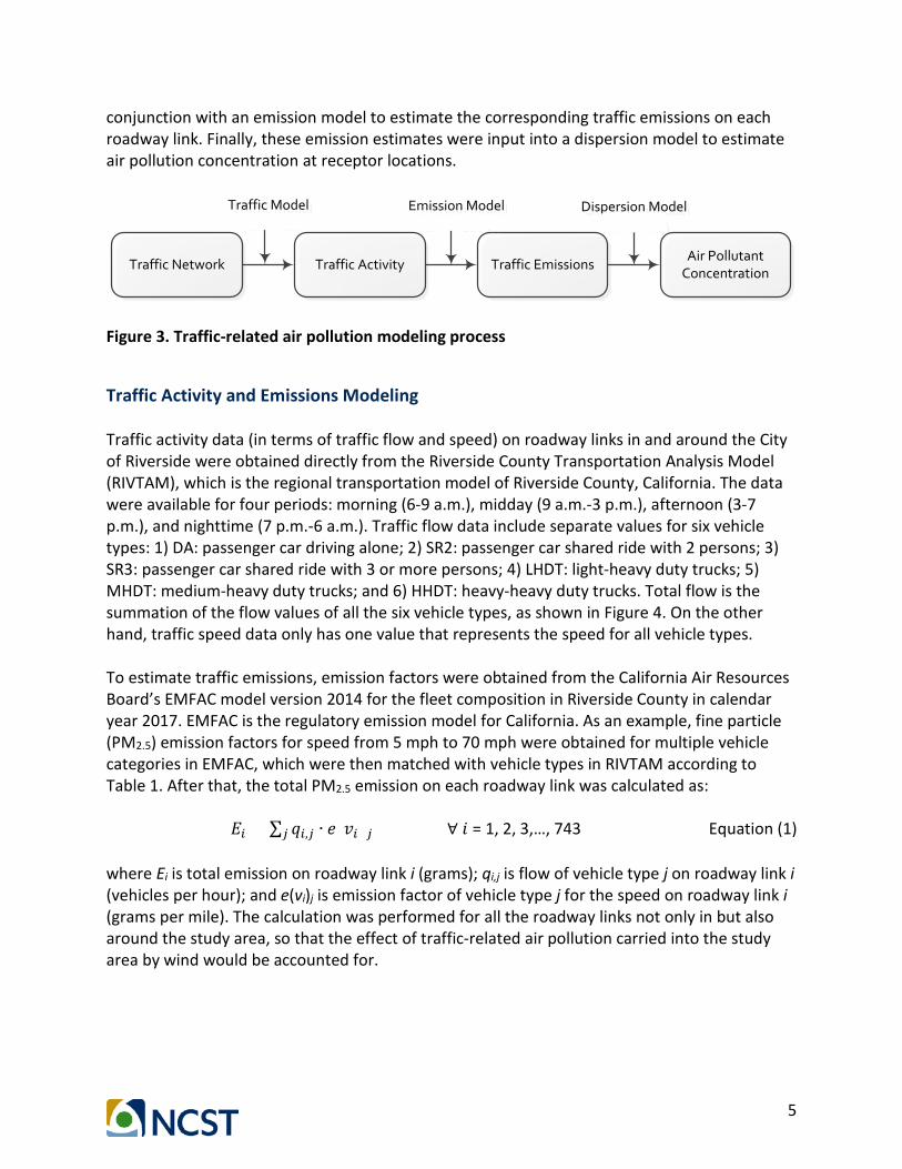
The air pollution concentration estimation process involves multiple steps, datasets, and modeling tools, as shown in Figure 3. First, a digital map of roadway network was used as the input for a traffic model to estimate traffic activity, in terms of flow and speed, on each roadway link in the network. Then, the estimated traffic flow and speed were used in

5

conjunction with an emission model to estimate the corresponding traffic emissions on each roadway link. Finally, these emission estimates were input into a dispersion model to estimate air pollution concentration at receptor locations.

Figure 3. Traffic-related air pollution modeling process

Traffic Activity and Emissions Modeling Traffic activity data (in terms of traffic flow and speed) on roadway links in and around the City of Riverside were obtained directly from the Riverside County Transportation Analysis Model (RIVTAM), which is the regional transportation model of Riverside County, California. The data were available for four periods: morning (6-9 a.m.), midday (9 a.m.-3 p.m.), afternoon (3-7 p.m.), and nighttime (7 p.m.-6 a.m.). Traffic flow data include separate values for six vehicle types: 1) DA: passenger car driving alone; 2) SR2: passenger car shared ride with 2 persons; 3) SR3: passenger car shared ride with 3 or more persons; 4) LHDT: light-heavy duty trucks; 5) MHDT: medium-heavy duty trucks; and 6) HHDT: heavy-heavy duty trucks. Total flow is the summation of the flow values of all the six vehicle types, as shown in Figure 4. On the other hand, traffic speed data only has one value that represents the speed for all vehicle types. To estimate traffic emissions, emission factors were obtained from the California Air Resources Board’s EMFAC model version 2014 for the fleet composition in Riverside County in calendar year 2017. EMFAC is the regulatory emission model for California. As an example, fine particle (PM2.5) emission factors for speed from 5 mph to 70 mph were obtained for multiple vehicle categories in EMFAC, which were then matched with vehicle types in RIVTAM according to Table 1. After that, the total PM2.5 emission on each roadway link was calculated as:

𝐸𝐸𝑖𝑖 = ∑ 𝑞𝑞𝑖𝑖,𝑗𝑗 ∙ 𝑒𝑒(𝑣𝑣𝑖𝑖)𝑗𝑗 ∀ 𝑖𝑖𝑗𝑗 = 1, 2, 3,…, 743 Equation (1) where Ei is total emission on roadway link i (grams); qi,j is flow of vehicle type j on roadway link i (vehicles per hour); and e(vi)j is emission factor of vehicle type j for the speed on roadway link i (grams per mile). The calculation was performed for all the roadway links not only in but also around the study area, so that the effect of traffic-related air pollution carried into the study area by wind would be accounted for.

Traffic Network Traffic Activity Traffic Emissions Air Pollutant

Concentration

Traffic Model(RIVTAM)

Traffic Model(RIVTAM)

Emission Model (EMFAC2007)

Emission Model (EMFAC2007)

Dispersion Model (CALINE4)

Dispersion Model (CALINE4)

6

Figure 4. Total flow (vehicles per hour) in the morning period Table 1. Vehicle type mapping

This Project RIVTAM EMFAC2014 LDV DA, SR2, SR3 LDA, LDT1, LDT2, MDV LHDT LHDT LHDT1, LHDT2 MHDT MHDT MHDT HHDT HHDT HHDT

Air Pollutant Dispersion Modeling Recently, the U.S. Environmental Protection Agency (EPA) released R-LINE, a research grade dispersion model for near-roadway assessments. It is based on a steady-state Gaussian formulation and is designed specifically to simulate air dispersion of emissions from line sources (3, 4). Compared to AERMOD, which is one of the air dispersion models

7

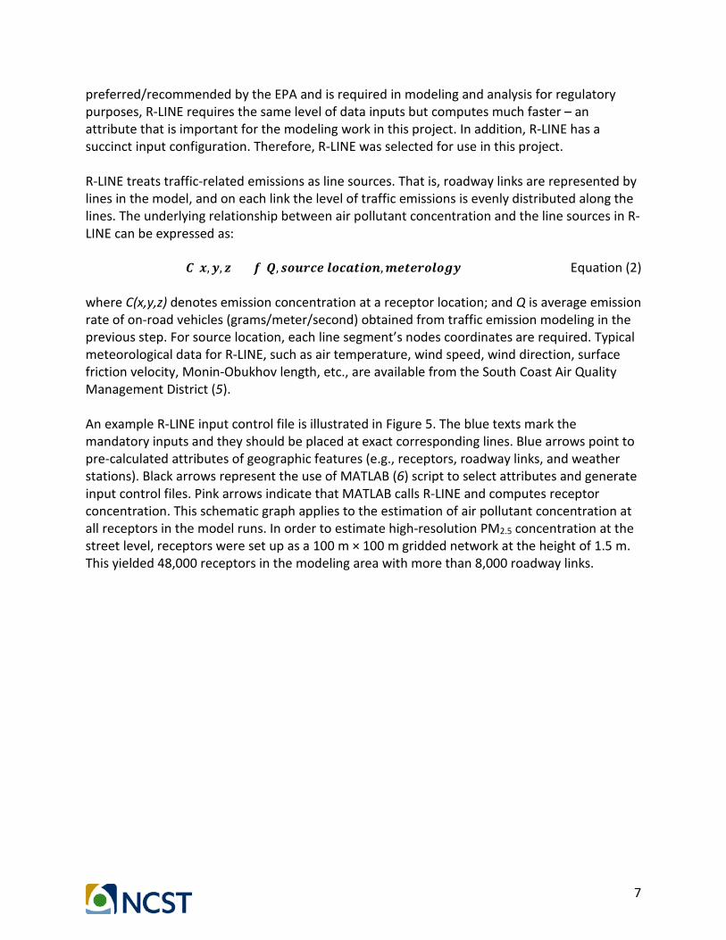
preferred/recommended by the EPA and is required in modeling and analysis for regulatory purposes, R-LINE requires the same level of data inputs but computes much faster – an attribute that is important for the modeling work in this project. In addition, R-LINE has a succinct input configuration. Therefore, R-LINE was selected for use in this project. R-LINE treats traffic-related emissions as line sources. That is, roadway links are represented by lines in the model, and on each link the level of traffic emissions is evenly distributed along the lines. The underlying relationship between air pollutant concentration and the line sources in R-LINE can be expressed as:

𝑪𝑪(𝒙𝒙,𝒚𝒚, 𝒛𝒛) = 𝒇𝒇(𝑸𝑸, 𝒔𝒔𝒔𝒔𝒔𝒔𝒔𝒔𝒔𝒔𝒔𝒔 𝒍𝒍𝒔𝒔𝒔𝒔𝒍𝒍𝒍𝒍𝒍𝒍𝒔𝒔𝒍𝒍,𝒎𝒎𝒔𝒔𝒍𝒍𝒔𝒔𝒔𝒔𝒔𝒔𝒍𝒍𝒔𝒔𝒎𝒎𝒚𝒚 ) Equation (2)

where C(x,y,z) denotes emission concentration at a receptor location; and Q is average emission rate of on-road vehicles (grams/meter/second) obtained from traffic emission modeling in the previous step. For source location, each line segment’s nodes coordinates are required. Typical meteorological data for R-LINE, such as air temperature, wind speed, wind direction, surface friction velocity, Monin-Obukhov length, etc., are available from the South Coast Air Quality Management District (5). An example R-LINE input control file is illustrated in Figure 5. The blue texts mark the mandatory inputs and they should be placed at exact corresponding lines. Blue arrows point to pre-calculated attributes of geographic features (e.g., receptors, roadway links, and weather stations). Black arrows represent the use of MATLAB (6) script to select attributes and generate input control files. Pink arrows indicate that MATLAB calls R-LINE and computes receptor concentration. This schematic graph applies to the estimation of air pollutant concentration at all receptors in the model runs. In order to estimate high-resolution PM2.5 concentration at the street level, receptors were set up as a 100 m × 100 m gridded network at the height of 1.5 m. This yielded 48,000 receptors in the modeling area with more than 8,000 roadway links.

8

Figure 5. Schematic graph of transition from spatial feature attributes to dispersion modeling implementation In regulatory analyses, it is desirable to use 5-year history of hourly meteorological data to calculate hourly average and maximum concentrations in order to capture any extreme concentration values that may result from certain meteorological conditions. That adds up to be a combination of 5 years x 365 days x 24 hours = 43,800 hourly meteorological scenarios. However, due to the large number of roadway links (more than 8,000) and receptors (48,000) in this project, it would be computationally expensive to calculate hourly concentrations for that many meteorological scenarios. In an effort to keep the computation time reasonable while still reasonably capturing extreme concentration values due to meteorological variation, we examined the meteorological variation across multiple years. The data of meteorological parameters are readily available from year 2008 to 2012. The analysis of these data for the five years revealed that the trends in weather patterns are similar across the years. For example, Figure 6 shows the average sensible heat flux (W/m2) for each time period and month from year 2009 to 2012, which are similar across the years. Hence, we used the meteorological data of year 2012 to represent the weather condition in the model year, which is 2017. The meteorology station is managed by South Coast Air Quality Management District and is located near Mt. Rubidoux in Riverside (5).

9

Figure 6. Average sensible heat flux (W/m2) for each period and month from 2009 to 2012 at Riverside Meteorology Station Also, we calculated the hourly average surface meteorological parameters for the following time scenarios: morning period (6:00 – 9:00), midday period (9:00 – 15:00), and afternoon period (15:00 – 18:00) for each month in year 2012, resulting in 36 scenarios in total. The nighttime period was not considered because bicycling activities are typically very low during nighttime. For example, to calculate hourly average surface meteorological parameters for the morning period in August 2012, we extracted hourly meteorological data for the 63 hours (3 hours in each day x 31 days in August), and calculated their average values. For wind speed, we used vector average. For scalar parameters such as air temperature and surface friction velocity, we used arithmetic average. We used this averaging strategy to calculate average morning, midday, and afternoon meteorological data for each month of 2012, which resulted in 36 meteorological scenarios. Then, we used the 36 sets of meteorological data to estimate hourly average PM2.5 concentrations. An example of hourly average values of meteorological parameters for the morning period in August 2012 are given in Table 2.

10

Table 2. Critical surface meteorological parameters and their hourly averaged values for morning period in August 2012

Parameter Value year 12 month 8 day 15 hour 6 sensible heat (W/m2) 40.34 u* - surface friction velocity (m/s) 0.11 w* - convective velocity scale (m/s) 0.7 VPTG - vertical potential temperature above Zic (K/m) 0.021 Zic - height of convectively-generated boundary layer (m) 245 Zim - height of mechanically-generated boundary layer (m) 110 L - Monin-Obukhov length (m) -100.8 Zo - surface roughness length (m) 0.314 Bo - Bowen ratio 1 Albedo 0.39 ws - reference wind speed (m/s) 0.2 wd – reference wind direction (degree) 132 zref - reference height for wind (m) 9.1 temp - reference emperature (K) 296 Ztemp - reference height for temperature (m) 5.5

During the modeling steps described above, data from different sources were extracted and computed on a link-by-link basis and parsed as binary files which could be directly manipulated by programming tools such as MATLAB. Using MATLAB scripts, model inputs including roadway geometry, emission factors, and meteorological data were written into text files and fed to the R-LINE program suite to calculate PM2.5 concentration values. Figure 7 shows a color map of PM2.5 concentrations in the City of Riverside during the morning period in August 2012, which is one of the 36 scenarios modeled in this project.

11

Figure 7. Estimated fine particle concentrations during the morning period in August

12

Generating Air Pollution Exposure Map for Bicycle Route Planning

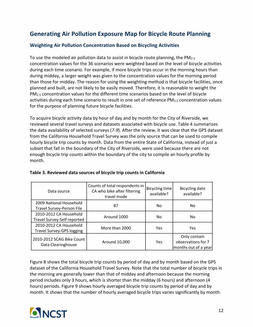
Weighting Air Pollution Concentration Based on Bicycling Activities To use the modeled air pollution data to assist in bicycle route planning, the PM2.5 concentration values for the 36 scenarios were weighted based on the level of bicycle activities during each time scenario. For example, if more bicycle trips occur in the morning hours than during midday, a larger weight was given to the concentration values for the morning period than those for midday. The reason for using the weighting method is that bicycle facilities, once planned and built, are not likely to be easily moved. Therefore, it is reasonable to weight the PM2.5 concentration values for the different time scenarios based on the level of bicycle activities during each time scenario to result in one set of reference PM2.5 concentration values for the purpose of planning future bicycle facilities. To acquire bicycle activity data by hour of day and by month for the City of Riverside, we reviewed several travel surveys and datasets associated with bicycle use. Table 4 summarizes the data availability of selected surveys (7-9). After the review, it was clear that the GPS dataset from the California Household Travel Survey was the only source that can be used to compile hourly bicycle trip counts by month. Data from the entire State of California, instead of just a subset that fall in the boundary of the City of Riverside, were used because there are not enough bicycle trip counts within the boundary of the city to compile an hourly profile by month. Table 3. Reviewed data sources of bicycle trip counts in California

Figure 8 shows the total bicycle trip counts by period of day and by month based on the GPS dataset of the California Household Travel Survey. Note that the total number of bicycle trips in the morning are generally lower than that of midday and afternoon because the morning period includes only 3 hours, which is shorter than the midday (6 hours) and afternoon (4 hours) periods. Figure 9 shows hourly averaged bicycle trip counts by period of day and by month. It shows that the number of hourly averaged bicycle trips varies significantly by month.

Data sourceCounts of total respondents in

CA who bike after filtering travel mode

Bicycling time available?

Bicycling date available?

2009 National Household Travel Survey-Person File 87 No No

2010-2012 CA Household Travel Survey-Self reported Around 1000 No No

2010-2012 CA Household Travel Survey-GPS logging More than 2000 Yes Yes

2010-2012 SCAG Bike Count Data Clearinghouse Around 10,000 Yes

Only containobservations for 7

months out of a year

13

Also, the number of hourly average bicycle trips does not show a trend by period of day. For example, we do not observe that there are more hourly bicycle trips on the road during the morning and afternoon periods than during the midday period, as it is for vehicular traffic.

Figure 8. Total bicycle trip counts by period of day and by month, based on 2010-12 California Household Travel Survey

Figure 9. Hourly averaged bicycle trip counts by period of day and by month, based on 2010-12 California Household Travel Survey

14

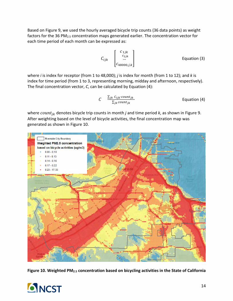
Based on Figure 9, we used the hourly averaged bicycle trip counts (36 data points) as weight factors for the 36 PM2.5 concentration maps generated earlier. The concentration vector for each time period of each month can be expressed as:

𝐶𝐶𝑖𝑖𝑗𝑗𝑖𝑖 = �𝑐𝑐1𝑗𝑗𝑖𝑖𝑐𝑐2𝑗𝑗𝑗𝑗…

𝑐𝑐48000,𝑗𝑗,𝑖𝑖

� Equation (3)

where i is index for receptor (from 1 to 48,000); j is index for month (from 1 to 12); and k is index for time period (from 1 to 3, representing morning, midday and afternoon, respectively). The final concentration vector, C, can be calculated by Equation (4):

𝐶𝐶 =∑ (𝐶𝐶𝑖𝑖𝑗𝑗𝑗𝑗∙𝑐𝑐𝑜𝑜𝑜𝑜𝑜𝑜𝑜𝑜𝑗𝑗𝑗𝑗)𝑗𝑗𝑗𝑗

∑ 𝑐𝑐𝑜𝑜𝑜𝑜𝑜𝑜𝑜𝑜𝑗𝑗𝑗𝑗𝑗𝑗𝑗𝑗 Equation (4)

where 𝑐𝑐𝑐𝑐𝑐𝑐𝑐𝑐𝑐𝑐𝑗𝑗𝑖𝑖 denotes bicycle trip counts in month j and time period k, as shown in Figure 9. After weighting based on the level of bicycle activities, the final concentration map was generated as shown in Figure 10.

Figure 10. Weighted PM2.5 concentration based on bicycling activities in the State of California

15

Mapping the Exposure to Near-Road Air Pollution Concentration Using the final PM2.5 concentration map (Figure 10), a bicyclist’s exposure to traffic-related air pollution on each roadway link in the City of Riverside can be calculated. The exposure scenario in this study is a bicyclist’s direct exposure to vehicular PM2.5 in a near-road outdoor microenvironment. We use inhaled mass as a metric for quantifying the level of exposure. It is a function of air pollutant concentration that the bicyclist is exposed to, duration of the exposure, and breathing rate of the bicyclist during the time of exposure. In this study, PM2.5 concentration was estimated for each roadway link. Therefore, inhaled mass of PM2.5 for bicyclist k traveling on roadway link i can be expressed as in Equation (5), assuming that the breathing rate of the bicyclist remains the same throughout the roadway link.

𝐼𝐼𝐼𝐼𝑖𝑖,𝑖𝑖 = 𝑐𝑐𝑖𝑖 ∙ 𝑐𝑐𝑖𝑖,𝑖𝑖 ∙ 𝐵𝐵𝐵𝐵𝑖𝑖,𝑖𝑖 Equation (5) where IM is inhaled mass of PM2.5 (µg); c is PM2.5 concentration (µg/m3) along the roadway link; t is travel duration (minutes); and BR is breathing rate of the bicyclist (m3/minute). c is calculated by first extracting the locations of vertices on each link and then determining the PM2.5 concentration at each location from the concentration map. Each link has at least 3 vertices (i.e., start point, midpoint, and end point), and c is calculated as the average of the concentration values at all the vertices. The bicycling duration on a roadway link was calculated based on the link length (meters) and the assumed speed of an average bicyclist of 9 miles per hour, which is based on the real-world data in the GPS dataset of the 2010-12 California Household Travel Survey. The breathing rate of an average bicyclist is assumed to be 0.04 m3/minute based on health studies (10-12). Figure 11 shows the level of exposure to PM2.5 for an average bicyclist on a link-by-link basis, where the inhaled mass values are normalized by link length. The color map is categorized by five quantiles based on the normalized exposure values and the number of links. As expected, the map shows that most of the links in the top 20% bracket (red color) are on, or in close proximity to, the two major freeways passing through the city—State Route 91 (SR-91) and State Route 60 (SR-60). However, it is observed that for the SR-91 corridor north of Arlington Avenue the red colored links are mostly on the west side of SR-91, while they are mostly on the east side of SR-91 for the corridor south of Arlington Ave. This may be due to the different wind directions in the area in the 36 different time periods. For the SR-60 corridor, most of the red colored links are south of the freeway. For non-freeway roads, the major arterials in the city—Magnolia Boulevard, Van Buren Blvd, and Arlington Ave—also have several links that are in the top 20% bracket. This information about potential exposure of bicyclists to harmful air pollution can be used in conjunction with other information pertinent to safety, connectivity, accessibility, and other metrics in the planning of new bicycle routes and facilities.

16

Figure 11. Traffic-related primary PM2.5 exposure per mile for bicyclists

Developing an Interactive Bicycle Route Planning Tool To develop an online tool for future bicycle facility planning, we have integrated the following map layers:

1. Traffic-related PM2.5 exposure for an average bicyclist, total inhaled mass, and inhaled mass normalized by link length, as shown in Figure 5. In addition, the road network map contains other information that are relevant in bicycle facility planning such as link length, roadway speed limit category, and whether a road divider(s) exists or not.

2. Existing bicycle facility map, which includes Class I bicycle paths along city roads, and Class II bicycle lanes that are already built in the City of Riverside up to year 2012 (based on Riverside’s Bicycle Master Plan years 2007 and 2012).

3. Historical bicycle crash data in year 2014 within the City of Riverside (based on California Highway Patrol - Statewide Integrated Traffic Records System (http://iswitrs.chp.ca.gov/Reports/jsp/userLogin.jsp). The map layer labels the accident

17

location, time, date, crash severity, vehicle at fault, parties involved, and main cause of the accident.

In addition, data regarding other bicyclist-friendly facilities within the city, for instance, Metrolink stations, bus stations, parks, etc., can be integrated as additional layers as well. The integrated data layers have been published online for demonstration purposes at http://arcg.is/29CESgp. As shown in Figure 12, the bicycle route planning support tool includes several functions to help users (e.g., planners or engineers) understand the data, for example:

1. Layer selection: Users can choose the layer(s) to be displayed. 2. Filter: Users can choose a layer and select roadway links whose attributes match

specified criteria.

3. Bookmark: Users can zoom to a bookmarked area of the city and view the map at a finer level of detail.

4. Directions: Users can query directions from location A to location B based on the least

travel duration. With the map layers provided, users can also plan routes based on other criteria such as level of exposure to air pollution and safety.

Figure 12. Bicycle route planning support tool

18

Case Studies of Considering Traffic-Related Air Pollution Exposure in Bicycle Route Planning According to the American Association of State Highway and Transportation Officials (AASHTO), the most important factors to be considered for bicycle planning include (13):

• User needs — Balancing the full range of needs of current and future bicyclists.

• Traffic volumes and speeds — Motor vehicle traffic volumes and speeds should be considered along with the roadway width. Some bicyclists will avoid roadways with high speeds and heavy volumes of traffic, unless they are provided with a facility that offers some degree of separation from traffic. By contrast, people who regularly use a bicycle for transportation often use main roadways because their directness and higher priority at intersections typically make them more efficient routes. In many cases, the best approach is to improve the arterial roadway to accommodate bicycles, but to also provide a parallel route along streets with lower speeds and traffic volumes.

• Overcoming barriers – Overcoming constraints and physical barriers such as freeways or

waterways should be a top priority when developing a bikeway network. A single major barrier (e.g., difficult intersection, bridge without sidewalks or bike lanes) can render an otherwise attractive bikeway corridor undesirable. Input from local bicyclists, along with a field analysis of major highway crossings, railroads, and river crossings, can help to identify major barriers.

• Connection to land uses – Bikeways should allow bicyclists to access key destinations.

They should connect to employment zones, parks, schools, shopping, restaurants, coffee and ice cream shops, sports facilities, community centers, major transit connections, and other land uses that form the fabric of a community.

• Directness of route – A bikeway should connect to desirable locations with as few detours

as possible. For example, does a bicyclist have to travel out of his or her way on a route with many turns to reach a safe freeway overpass? Multiple turns can disorient a rider and unnecessarily complicate and lengthen a trip.

• Logical route – Does the planned network make sense? A network should include facilities

that bicyclists already use, or have expressed interest in using.

• Intersections – Bikeways should be planned to allow for as few stops as possible, as bicycling efficiency is greatly reduced by stops and starts. If bicyclists are required to make frequent stops, for example, along streets with stop signs every block, they may avoid the route or disregard traffic control devices. Signalized intersections with very short green times (such as those on low-priority streets) can lead to disregard for traffic control. At

19

major streets, crossings should be carefully planned and managed to ensure maximum safety and flow.

• Aesthetics — Scenery is an important consideration along a facility, particularly for a

facility that will serve a primarily recreational purpose. Trees can also provide cooler riding conditions in summer and can provide a windbreak. Bicyclists tend to favor roads with adjacent land uses that are attractive such as campuses, shopping districts, and those with scenic views.

• Spacing or density of bikeways – A bikeway network should be planned for maximum use

and comfort, and thus should provide an appropriate density relative to local conditions. Some bicycle network plans have set a goal to provide a bicycle facility within one-fourth of a mile of every resident.

• Overall feasibility — Decisions regarding the location of new bikeways may also include

an overall assessment of feasibility given physical or right-of-way constraints, as well as other factors that may impact the cost of the project. While funding availability may influence decisions, it is essential that a lack of funds not result in a poorly-designed or constructed facility. The decision to implement a bikeway plan should also be made with a conscious, long-term commitment to a proper level of maintenance. Facility selection should seek to maximize user benefit per dollar funded.

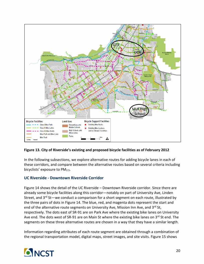
In this section, we use the estimated PM2.5 concentration data to demonstrate the incorporation of bicyclists’ exposure to traffic-related air pollution in the planning of two bicycle routes in the City of Riverside, California. The City last updated its Bicycle Master Plan in 2012 (14). Figure 13 shows the existing and proposed bicycle facilities in the City as of February 2012. A meeting was held with the City’s Bicycle Program Coordinator to discuss potential case studies for use in this research. Two candidate corridors were identified, as circled in Figure 13.

1. University of California at Riverside (UCR) – Downtown Riverside (DTR) corridor: This corridor connects the two major trip origins/destinations in the city with potential for having high bicycle mode share. Currently, there exist bike lanes on University Ave between UCR and a MetroLink (commuter train) station just east of the SR-91 freeway. The 2012 Bicycle Master Plan Update proposed extending the bike lanes on University Ave into the downtown area.

2. Van Buren corridor around Martin Luther King (MLK) High School: This area has a high number of bicycle-related accidents, steep road grade, and high roadway intersection density, which pose challenges to bicyclists. Currently, there exist bike lanes on Van Buren Blvd east of MLK High School. The 2012 Bicycle Master Plan Update proposed extending these bike lanes further west.

20

Figure 13. City of Riverside’s existing and proposed bicycle facilities as of February 2012 In the following subsections, we explore alternative routes for adding bicycle lanes in each of these corridors, and compare between the alternative routes based on several criteria including bicyclists’ exposure to PM2.5.

UC Riverside - Downtown Riverside Corridor Figure 14 shows the detail of the UC Riverside – Downtown Riverside corridor. Since there are already some bicycle facilities along this corridor—notably on part of University Ave, Linden Street, and 3rd St—we conduct a comparison for a short segment on each route, illustrated by the three pairs of dots in Figure 14. The blue, red, and magenta dots represent the start and end of the alternative route segments on University Ave, Mission Inn Ave, and 3rd St, respectively. The dots east of SR-91 are on Park Ave where the existing bike lanes on University Ave end. The dots west of SR-91 are on Main St where the existing bike lanes on 3rd St end. The segments on these three alternative routes are chosen in a way that they have a similar length. Information regarding attributes of each route segment are obtained through a combination of the regional transportation model, digital maps, street images, and site visits. Figure 15 shows

UCR

DTR

MLK High School

21

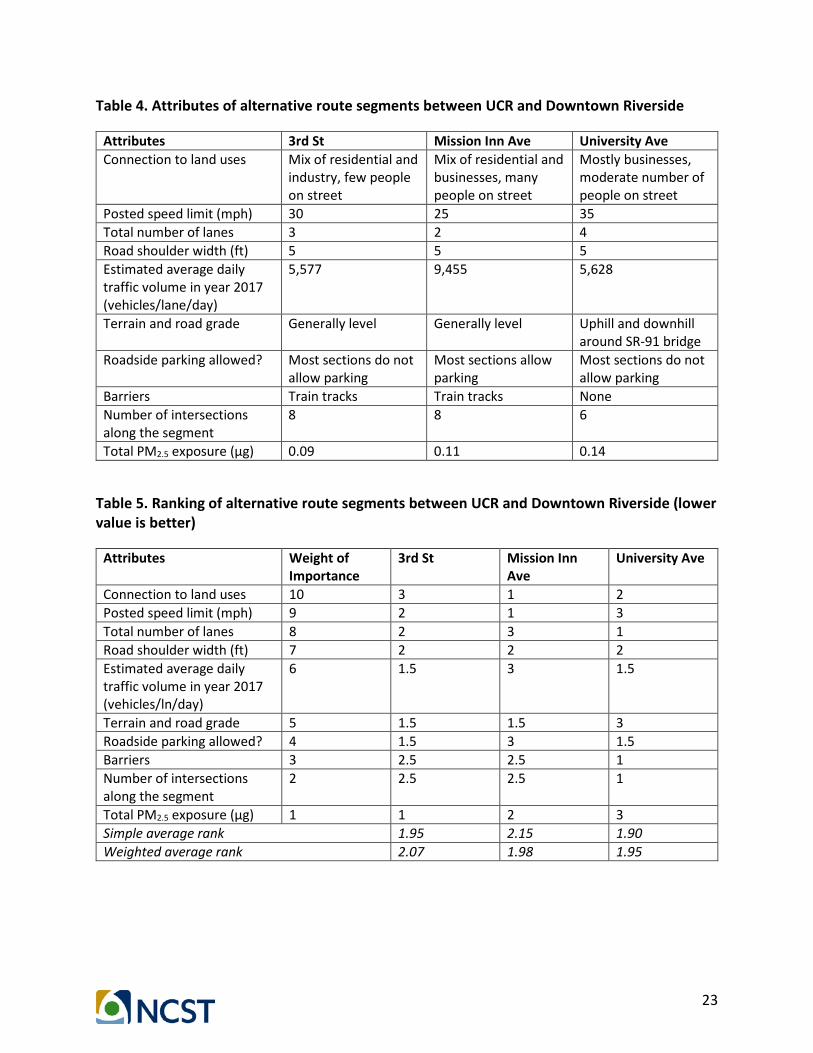
an example street image on each of the three alternative route segments. Then, Table 4 lists key attributes of each route segment that are related to the factors that should be considered when planning bicycle routes. Some of the attribute values are qualitative, therefore when comparing the attribute values among the three alternatives, it is appropriate to use an ordinal scale or rank order (1st, 2nd, 3rd, …).

Figure 14. Alternative bicycle routes between UCR and Downtown Riverside Table 5 shows the ranking of the three alternative route segments. For each attribute, such as posted speed limit, the three alternative route segments are ranked from 1 to 3, where 1 is the best and 3 is the worst. As an example, for the posted speed limit, Mission Inn Ave is ranked 1 as it has the lowest posted speed limit (25 mph) while University Ave is ranked 3 as it has the highest posted speed limit (35 mph). For some attributes, the ranking may be tied. For example, in the case of terrain and road grade both 3rd St and Mission Inn Ave are both level in general, whereas University Ave has uphill and downhill around the SR-91 overpass. In this case, University Ave is ranked 3 and the other two routes share the rank of 1.5. Similarly, in the case of barriers where both 3rd St and Mission Inn Ave have train tracks while University Ave does not, University Ave is ranked 1 and the other two routes share the rank of 2.5, which is the average of 2 and 3. Also given in Table 5 is the weight of importance of each attribute. The weight is also based on an ordinal scale from 1 to 10, with a higher weight being more important.

Downtown Riverside

University Ave

3rd St

Linden St

UC Riverside

22

a) 3rd St

b) Mission Inn Ave

c) University Ave Figure 15. Street images of the alternative route segments between UCR and Downtown Riverside

23

Table 4. Attributes of alternative route segments between UCR and Downtown Riverside

Attributes 3rd St Mission Inn Ave University Ave Connection to land uses Mix of residential and

industry, few people on street

Mix of residential and businesses, many people on street

Mostly businesses, moderate number of people on street

Posted speed limit (mph) 30 25 35 Total number of lanes 3 2 4 Road shoulder width (ft) 5 5 5 Estimated average daily traffic volume in year 2017 (vehicles/lane/day)

5,577 9,455 5,628

Terrain and road grade Generally level Generally level Uphill and downhill around SR-91 bridge

Roadside parking allowed? Most sections do not allow parking

Most sections allow parking

Most sections do not allow parking

Barriers Train tracks Train tracks None Number of intersections along the segment

8 8 6

Total PM2.5 exposure (µg) 0.09 0.11 0.14 Table 5. Ranking of alternative route segments between UCR and Downtown Riverside (lower value is better)

Attributes Weight of Importance

3rd St Mission Inn Ave

University Ave

Connection to land uses 10 3 1 2 Posted speed limit (mph) 9 2 1 3 Total number of lanes 8 2 3 1 Road shoulder width (ft) 7 2 2 2 Estimated average daily traffic volume in year 2017 (vehicles/ln/day)

6 1.5 3 1.5

Terrain and road grade 5 1.5 1.5 3 Roadside parking allowed? 4 1.5 3 1.5 Barriers 3 2.5 2.5 1 Number of intersections along the segment

2 2.5 2.5 1

Total PM2.5 exposure (µg) 1 1 2 3 Simple average rank 1.95 2.15 1.90 Weighted average rank 2.07 1.98 1.95

24

In Table 5 there are two types of average rank: 1) simple average rank, and 2) weighted average rank. They are calculated as:

𝑆𝑆𝑖𝑖𝑆𝑆𝑆𝑆𝑆𝑆𝑒𝑒 𝑎𝑎𝑣𝑣𝑒𝑒𝑎𝑎𝑎𝑎𝑎𝑎𝑒𝑒 𝑎𝑎𝑎𝑎𝑐𝑐𝑟𝑟 = 1𝑁𝑁∑ 𝑎𝑎𝑖𝑖𝑁𝑁𝑖𝑖=1 Equation (6)

𝑊𝑊𝑒𝑒𝑖𝑖𝑎𝑎ℎ𝑐𝑐𝑒𝑒𝑡𝑡 𝑎𝑎𝑣𝑣𝑒𝑒𝑎𝑎𝑎𝑎𝑎𝑎𝑒𝑒 𝑎𝑎𝑎𝑎𝑐𝑐𝑟𝑟 = ∑ (𝑟𝑟𝑖𝑖∙𝑤𝑤𝑖𝑖)𝑁𝑁𝑖𝑖=1∑ 𝑤𝑤𝑖𝑖𝑁𝑁𝑖𝑖=1

Equation (7)

where ri is rank of attribute i; wi is weight of attribute i; and N is number of attributes. The calculation of the simple average rank implies that all the attributes have equal weight or importance. Figure 16 shows the simple average rank values of the three alternative route segments with and without the total PM2.5 exposure attribute. Based on this figure, University Ave would be the best alternative regardless of the exposure to PM2.5 is taken into account or not.

Figure 16. Simple average rank of the alternative route segments between UCR and Downtown Riverside When looking at the weighted average rank shown in Table 5, University Ave would again be the best alternative as it has the lowest rank value. This weighted average ranking is based on the weight of importance listed in Table 5 where the total PM2.5 exposure attribute is given the least importance (weight = 1). Figure 17 examines the impact of changing the weight of the PM2.5 exposure attribute. As an example, if the PM2.5 exposure attribute is considered to be the second least important, its weight will become 2 and the weight of the number of intersections attribute will become 1 instead. Likewise, if the PM2.5 exposure attribute is considered to be the third least important, its weight will become 3 and the weight of the barriers attribute will become 2 and the number of intersections attribute will become 1. And if the PM2.5 exposure

25

attribute is considered to be the most important, its weight will become 10 and the weight of all the other attributes will be lowered by one accordingly.

Figure 17. Weighted average rank of the alternative route segments between UCR and Downtown Riverside

Based on Figure 17, University Ave would be the best alternative if the weight of the PM2.5 exposure attribute is 1, as in Table 5. However, Mission Inn Ave would become the best alternative if the weight of the PM2.5 exposure attribute is between 2 and 9. If the weight of the PM2.5 exposure attribute is 10, then 3rd St would become the best alternative. As indicated earlier and shown in Figure 14, there are already bike lanes on 3rd St, which are part of the gridded bicycle facility network of the city. 3rd St is included in this case study for comparison purposes only. On the other hand, there are no existing bike lanes on either University Ave or Mission Inn Ave, and the two streets are just a block away from each other. Both streets offer connection to another major area where Mission Inn Ave extends further west across Santa Ana River into the City of Rubidoux, while University Ave extends into the east side of the City of Riverside to UCR. Both will be a natural alternative for forming part of the gridded bicycle facility network of the city. Therefore, they are truly competing alternatives for building bike lanes. Based on the information in Table 4, both streets have pros and cons. The results in Figure 17 indicate that either street would be a suitable candidate depending on whether exposure to traffic-related air pollution is taken into consideration and how important this factor is relative to other factors. Figure 16 and Figure 17 illustrate an example of how the consideration of exposure to traffic-related air pollution could impact the outcome of bicycle route planning. It is noted that the bicycle route planning process may vary from one city to another, and planners/engineers in different cities may elect to use the information about exposure to traffic-related air pollution differently. For instance, both the order and the weight of importance for the different

26

attributes can be altered in many ways, which may affect the ranking results. Planners/engineers and stakeholders may jointly determine how important the different attributes, including exposure to traffic-related air pollution, are relative to one another. It is also noted that the illustration in this case study does not necessarily include all factors that may be considered. In other areas or cities, there may be other unique factors that should also be taken into consideration in the bicycle route planning.

Van Buren Corridor around Martin Luther King High School The Van Buren corridor around Martin Luther King (MLK) High School has many schools and residential communities. Also, this area has a high number of bicycle-related accidents, steep road grade, and high roadway intersection density, making it an interesting case study. Currently, bike lanes exist on Van Buren Blvd east of MLK High School. The 2012 Bicycle Master Plan Update proposed extending these bike lanes further west, as shown in Figure 18. The planned bicycle lanes include a segment on Van Buren Blvd from the end of the existing bike lanes to the intersection with Washington St, as represented by the two orange dots. An alternative is a parallel segment on Krameria Ave south of Van Buren Blvd, as represented by the two red dots. The red dot on the east end is about 2,000 ft south of the orange dot on the east, while the red dot on the west is about 1,000 ft south of the orange dot on the west end.

Figure 18. Alternative bicycle routes along Van Buren corridor around MLK High School

27

Information regarding attributes of each route segment are gathered from the regional transportation model, digital maps, street images, and site visits. Figure 19 shows an example street image of each route segment. Table 6 then lists key attributes of each route segment that are related to the factors that should be considered when planning bicycle routes. Table 7 shows the ranking of the two alternative route segments.

a) Van Buren Blvd

b) Krameria Ave Figure 19. Street images of the alternative route segments around MLK High School

28

Table 6. Attributes of alternative route segments around MLK High School

Attributes Van Buren Blvd Krameria Ave Connection to land uses Mostly businesses Mostly residential Posted speed limit (mph) 50 25 Total number of lanes 4 1-2 Road shoulder width (ft) 3-5 2-5 Estimated average daily traffic volume in year 2017 (vehicles/lane/day)

7,689 1,578

Terrain and road grade Moderate road grade Moderate road grade Roadside parking allowed? Mostly no Parking is allowed on some of

the residential sections Barriers None None Number of intersections along the segment

11 12

Total PM2.5 exposure (µg) 0.2 0.07 Table 7. Ranking of alternative route segments around MLK High School (lower value is better)

Attributes Weight of

Importance Van Buren Blvd Krameria Ave

Connection to land uses 10 1.5 1.5 Posted speed limit (mph) 9 2 1 Total number of lanes 8 1 2 Road shoulder width (ft) 7 1.5 1.5 Estimated average daily traffic volume in year 2017 (vehicles/lane/day)

6 2 1

Terrain and road grade 5 1.5 1.5 Roadside parking allowed? 4 1 2 Barriers 3 1.5 1.5 Number of intersections along the segment

2 1 2

Total PM2.5 exposure (µg) 1 2 1 Simple average rank 1.50 1.50 Weighted average rank 1.52 1.48

Using the same methodology as in the previous case study, the simple average and weighted average ranks are calculated. Figure 20 shows the simple average rank values of the two alternative route segments with and without the total PM2.5 exposure attribute. It is found that without considering the exposure to PM2.5, Van Buren Blvd would be a better alternative. But when taking such exposure into account, both route segments would be equally appropriate. This is not surprising as the total PM2.5 exposure on Van Buren Blvd is higher than that on Krameria Ave.

29

Figure 20. Simple average rank of the alternative route segments around MLK High School According to the weighted average rank in Table 7, Krameria Ave would be a better alternative by a slight margin when the total PM2.5 exposure attribute is the least important factor (weight = 1). Figure 21 shows the impact of increasing the weight of the PM2.5 exposure attribute. According to this figure, Krameria Ave would always be the better alternative no matter how much weight is given to the PM2.5 exposure attribute, as long as it is taken into consideration. The higher the weight is the bigger the margin between Krameria Ave and Van Buren Blvd. This is due to Krameria Ave having a lower PM2.5 exposure than Van Buren Blvd.

Figure 21. Weighted average rank of the alternative route segments around MLK High School

1.2

1.3

1.4

1.5

1.6

1.7

1.8

1 2 3 4 5 6 7 8 9 10

Rank

Weight of Air Pollution Exposure Metric (10 = Most Important)

Weighted Average RankVan Buren Blvd Krameria Ave

30

When looking at the two alternative route segments in Figure 18 from the bicycle facility network perspective, they are not directly competing with each other. Van Buren Blvd would be a more natural fit for expanding the bicycle facility network in the city as it is a major arterial with many businesses. Bicyclists who want to access the amenities on Van Buren Blvd or want to travel to destinations west of the end of the existing bike lanes could benefit from extended bike lanes on this route. However, there are many schools south of Van Buren Blvd, including Woodcrest Christian School, MLK High School, Mark Twain Elementary School, and Frank Augustus Miller Middle School. For children attending these schools, Krameria Ave would be a safer and lower air pollution exposure route for them to bike to school. Adding bike lanes on this route could potentially encourage residents, especially school-aged children and their parents, to ride bicycles more. Thus, in this case study, adding bike lanes on both routes would be ideal where the bike lanes on each route would serve different types of users making different types of trip.

31

Concluding Remarks Active transportation modes such as walking and biking are key elements of sustainable transportation systems. In order to promote biking as an alternative form of transportation, a holistic approach to improving the quality of biking experience is needed. The planning of bicycle routes typically takes into consideration available right-of-way, existing roadway infrastructure, vehicular traffic volume, safety concerns, and built environment, among others. Exposure to traffic-related air pollution, on the other hand, is rarely considered despite bicyclists being vulnerable to the harmful air pollution due to their direct exposure to vehicular exhaust and increased breathing rate during biking. This research attempts to fill this gap by developing a method to incorporate reduced exposure to traffic-related air pollution as another consideration in the bicycle route planning process in order to improve the quality of the biking experience and promote active travel. Current air quality measurement data are not available at the spatial resolution necessary for the planning of bicycle routes. In this research, high-resolution traffic-related air pollution concentrations were estimated through a modeling process that involves traffic activity, traffic emission, and air pollutant dispersion modeling. The modeling process was applied to estimate traffic-related primary fine particle (PM2.5) concentrations in the City of Riverside, California, for traffic volumes in calendar year 2017 based on a total of 36 hourly average meteorological conditions consisting of three time periods of day (morning, midday, and afternoon) for the 12 months in calendar year 2012. The 36 sets of estimated PM2.5 concentration values were then weighted by the level of bicycle activities by time period of day and by month of year derived from the GPS dataset in the 2010-12 California Household Travel Survey. This resulted in a weighted average PM2.5 concentration map for the city, based on which the level of exposure to PM2.5 for bicyclists was estimated for each roadway link in the city. Two case studies in the City of Riverside were used to demonstrate the consideration of traffic-related air pollution exposure in bicycle route planning. In each case study, alternative routes along the same travel corridor were analyzed with respect to 10 factors including connection to land uses, posted speed limit, total number of lanes, road shoulder width, traffic volume, terrain and road grade, roadside parking, presence of barriers, number of intersections, and total PM2.5 exposure. As some of these factors are qualitative, the comparison between the alternative routes was made by rank order. The use of equal, as well as different, weight of importance for each factor was evaluated. In terms of exposure to traffic-related air pollution, the comparison results reveal that the best alternative route depends on whether this factor is taken into consideration and how important this factor is relative to other factors. This research has developed a method for incorporating exposure to traffic-related air pollution as another consideration in the bicycle route planning process and has demonstrated how to apply the method through two case studies. Planners and engineers may elect to adopt the presented method or use the information about exposure to traffic-related air pollution differently. For instance, both the order and the weight of importance for the different factors

32

can be changed, which may affect the ranking results. Planners/engineers and stakeholders may jointly determine how important the different factors, including exposure to traffic-related air pollution, are in relation to one another. Other factors that should be taken into consideration for a specific corridor or area may also be included. Several aspects of this research can be improved and expanded in the future, for instance, including other sources of emissions and background concentration. Also, the biking speed and breathing rate assumptions can be refined by using values specific to demographic groups such as school-aged children and by accounting for waiting time at crossings and intersections. And if air quality measurement data become available at the necessary spatial resolution, they can be used in lieu of the estimated values in the bicycle route planning process directly.

33

References

1. Woodcock, J., Edwards, P., Tonne, C., Armstrong, B.G., Ashiru, O., Banister, D., Beevers, S., Chalabi, Z., Chowdhury, Z., Cohen, A., 2009. Public health benefits of strategies to reduce greenhouse-gas emissions: urban land transport. The Lancet, 374(9705), 1930-1943.

2. Maizlish, N., Woodcock, J., Co, S., Ostro, B., Fanai, A., Fairley, D., 2013. Health cobenefits and transportation-related reductions in greenhouse gas emissions in the San Francisco Bay area. American Journal of Public Health, 103(4), 703-709.

3. Community Modeling & Analysis System, R-LINE. https://www.cmascenter.org/r-line/. 4. Snyder, M. and H. David. User Guide for R-LINE Model 1.2. USEPA/ORD/NERLMD-81.

Atmospheric Exposure Research Branch, Atmospheric Modeling and Analysis Division, Research Triangle Park, NC, 2013

5. South Coast Air Quality Management District, Meteorological Data for AERMOD. http://www.aqmd.gov/home/library/air-quality-data-studies/meteorological-data/data-for-aermod.

6. MathWorks, Matlab: The language of technical computing. http://www.mathworks.com/products/matlab/.

7. National Household Travel Survey, 2009 National Household Travel Survey. http://nhts.ornl.gov/download.shtml

8. National Renewable Energy Laboratory, 2010-2012 California Household Travel Survey Transportation Secure Data Center. http://www.nrel.gov/transportation/secure_transportation_data.html

9. Southern California Association of Governments, 2010-2012 SCAG Bike Count Data Clearinghouse. http://www.bikecounts.luskin.ucla.edu/Download_Data.aspx.

10. Adams, W. Measurement of breathing rate and volume in routinely performed daily activities, Final report. Prepared for the California Air Resources Board, Contract, No. A033-205. Human Performance Laboratory, Physical Education Department, University of California, Davis, 1993. http://www.arb.ca.gov/research/single-project.php?row_id=64931.

11. Lucía, A., Carvajal, A., Calderón, F.J., Alfonso, A., Chicharro, J.L., 1999. Breathing pattern in highly competitive cyclists during incremental exercise. European journal of applied physiology and occupational physiology 79 (6), 512-521.

12. Pankow, J., Figliozzi, M., and Bigazzi, A., 2014. Evaluation of Bicyclists Exposure to Traffic-Related Air Pollution along Distinct Facility Types. NITC-RR-560. Portland, OR: Transportation Research and Education Center (TREC). http://dx.doi.org/10.15760/trec.121

13. American Association of State Highway and Transportation Officials (2012), AASHTO Guide for the Development of Bicycle Facilities, 4th Edition.

14. City of Riverside (2012). City of Riverside Bicycle Master Plan Update, March.

DISCLAIMER STATEMENT

This document is disseminated in the interest of information exchange. The contents of this report reflect the views of the authors who are responsible for the facts and accuracy of the data presented herein. The contents do not necessarily reflect the official views or policies of the State of California or the Federal Highway Administration. This publication does not constitute a standard, specification or regulation. This report does not constitute an endorsement by the Department of any product described herein. For individuals with sensory disabilities, this document is available in alternate formats. For information, call (916) 654-8899, TTY 711, or write to California Department of Transportation, Division of Research, Innovation and System Information, MS-83, P.O. Box 942873, Sacramento, CA 94273-0001.

Biking in Fresh Air: Consideration of Exposure to Traffic-Related Air Pollution in Bicycle Route Planning

March 2017 A Research Report from the National Center for Sustainable Transportation

Kanok Boriboonsomsin, University of California at Riverside

Jill Luo, University of California at Riverside

About the National Center for Sustainable Transportation The National Center for Sustainable Transportation is a consortium of leading universities committed to advancing an environmentally sustainable transportation system through cutting-edge research, direct policy engagement, and education of our future leaders. Consortium members include: University of California, Davis; University of California, Riverside; University of Southern California; California State University, Long Beach; Georgia Institute of Technology; and University of Vermont. More information can be found at: ncst.ucdavis.edu. Disclaimer The contents of this report reflect the views of the authors, who are responsible for the facts and the accuracy of the information presented herein. This document is disseminated under the sponsorship of the United States Department of Transportation’s University Transportation Centers program, in the interest of information exchange. The U.S. Government and the State of California assumes no liability for the contents or use thereof. Nor does the content necessarily reflect the official views or policies of the U.S. Government and the State of California. This report does not constitute a standard, specification, or regulation. Acknowledgments This study was funded by a grant from the National Center for Sustainable Transportation (NCST), supported by USDOT and Caltrans through the University Transportation Centers program. The authors would like to thank the NCST, USDOT, and Caltrans for their support of university-based research in transportation, and especially for the funding provided in support of this project. The authors also would like to thank Project Panel members—Lauren Iacobucci and Deborah Lynch of Caltrans, Jeanie Ward-Waller of California Bicycle Coalition, Jillian Wong of South Coast Air Quality Management District, and Marvel Norman of Inland Empire Biking Alliance—as well as Nathan Mustafa of the City of Riverside for their valuable input and assistance.

i

Biking in Fresh Air: Consideration of Exposure to Traffic-Related Air Pollution in

Bicycle Route Planning A National Center for Sustainable Transportation Research Report

March 2017

Kanok Boriboonsomsin and Jill Luo

College of Engineering - Center for Environmental Research and Technology, University of California at Riverside

ii

[page left intentionally blank]

iii

TABLE OF CONTENTS Introduction .................................................................................................................................... 1

Research Goal and Objectives .................................................................................................... 1

Estimation of Near-Road Air Pollutant Concentration ................................................................... 3

Scoping ........................................................................................................................................ 3

Traffic Activity and Emissions Modeling ..................................................................................... 5

Air Pollutant Dispersion Modeling .............................................................................................. 6

Generating Air Pollution Exposure Map for Bicycle Route Planning ............................................ 12

Weighting Air Pollution Concentration Based on Bicycling Activities ...................................... 12

Mapping Near-Road Air Pollution Concentration Exposure ..................................................... 15

Developing an Interactive Bicycle Route Planning Tool ........................................................... 16

Case Studies of Considering Traffic-Related Air Pollution Exposure in Bicycle Route Planning... 18

UC Riverside - Downtown Riverside Corridor ........................................................................... 20

Van Buren Corridor around Martin Luther King High School ................................................... 26

Concluding Remarks...................................................................................................................... 31

References .................................................................................................................................... 33

iv

Biking in Fresh Air: Consideration of Exposure to Traffic-Related Air Pollution in Bicycle Route Planning EXECUTIVE SUMMARY Active transportation modes such as walking and biking are key elements of sustainable transportation systems. In order to promote biking as an alternative form of transportation, a holistic approach to improving the quality of the biking experience is needed. The planning of bicycle routes typically takes into consideration available right-of-way, existing roadway infrastructure, vehicular traffic volume, safety concerns, and built environment, among others. Exposure to traffic-related air pollution, on the other hand, is rarely considered despite bicyclists being vulnerable to the harmful air pollution due to their direct exposure to vehicular exhaust and increased breathing rate during biking. This research attempts to fill this gap by developing a method to incorporate reduced exposure to traffic-related air pollution as another consideration in the bicycle route planning process in order to improve the quality of the biking experience and promote active travel. Current air quality measurement data are not available at the spatial resolution necessary for the planning of bicycle routes. In this research, high-resolution traffic-related air pollution concentrations were estimated through a modeling process that involves traffic activity, traffic emission, and air pollutant dispersion modeling. The modeling process was applied to estimate traffic-related primary fine particle (PM2.5) concentrations in the City of Riverside, California, for traffic volumes in calendar year 2017 based on a total of 36 hourly average meteorological conditions consisting of three time periods of day (morning, midday, and afternoon) for the 12 months in calendar year 2012. The 36 sets of estimated PM2.5 concentration values were then weighted by the level of bicycle activities by time period of day and by month of year derived from the GPS dataset in the 2010-12 California Household Travel Survey. This resulted in a weighted average PM2.5 concentration map for the city, based on which the level of exposure to PM2.5 for bicyclists was estimated for each roadway link in the city. Two case studies in the City of Riverside were used to demonstrate the consideration of traffic-related air pollution exposure in bicycle route planning. In each case study, alternative routes along the same travel corridor were analyzed with respect to 10 factors including connection to land uses, posted speed limit, total number of lanes, road shoulder width, traffic volume, terrain and road grade, roadside parking, presence of barriers, number of intersections, and total PM2.5 exposure. As some of these factors are qualitative, the comparison between the alternative routes was made by rank order. The use of equal, as well as different, weight of importance for each factor was evaluated. In terms of exposure to traffic-related air pollution, the comparison results reveal that the best alternative route depends on whether this factor is taken into consideration and how important this factor is relative to other factors.

v

This research has developed a method for incorporating exposure to traffic-related air pollution as another consideration in the bicycle route planning process and has demonstrated how to apply the method through two case studies. Planners and engineers may elect to adopt the presented method or use the information about exposure to traffic-related air pollution differently. For instance, both the order and the weight of importance for the different factors can be changed, which may affect the ranking results. Planners/engineers and stakeholders may jointly determine how important the different factors, including exposure to traffic-related air pollution, are in relation to one another. Other factors that should be taken into consideration for a specific corridor or area may also be included. Several aspects of this research can be improved and expanded in the future, for instance, including other sources of emissions and background concentration. Also, the biking speed and breathing rate assumptions can be refined by using values specific to demographic groups such as school-aged children and by accounting for waiting time at crossings and intersections. And if air quality measurement data become available at the necessary spatial resolution, they can be used in lieu of the estimated values in the bicycle route planning process directly. Lastly, the methodological framework developed in this research can be applied to other areas if the required data inputs are available for those areas.

1

Introduction Active transportation modes such as walking and biking are key elements of sustainable transportation systems. Biking is advocated as a way to mitigate local street congestion, foster community livability, and boost local economy. In addition, biking is also a form of exercise that helps keep physical fitness and prevent diseases. From a mode choice perspective, it may be argued that exposure to traffic-related emissions could be one factor that makes biking less appealing to travelers (i.e., a “disutility”). As a result, they would have another reason to be more inclined toward the use of automobiles, contributing to an increase in vehicle traffic and the associated air pollution in the process. In order to promote biking as an alternative form of transportation, a holistic approach to improving the quality of biking experience is needed. This includes, for example, providing route access to a variety of destinations, dedicating spaces for bicycle parking, ensuring a safe biking environment, and maintaining bicycle infrastructure. Local, regional, and state agencies in California are making efforts to increase bicycle infrastructure in the State in order to promote sustainable and multi-modal transportation. In most areas, bicycle routes are a subset of vehicle routes and new bicycle infrastructure is created by adding bicycle lane(s) to existing rights-of-way. The planning of bicycle routes typically takes into consideration available right-of-way, existing roadway infrastructure, vehicular traffic volume, safety concerns, and built environment, among others. Exposure to traffic-related air pollution, on the other hand, is rarely considered in route planning. However, bicyclists are the most vulnerable to the harmful air pollution due to their direct exposure to vehicular exhaust and increased breathing rate during biking. Traffic volume alone is not a sufficient surrogate for the level of air pollution on the road, though; it also depends on traffic speed, fleet mix, meteorology condition (e.g., wind speed and wind direction), and terrain. It is noteworthy to point out that, at the system levels (city, county, or national level) in developed countries where vehicle emissions are strictly controlled, encouraging active transportation far outweighs the risk from exposure to air pollutants and traffic-related injuries and death (1, 2). For individual active travelers, however, the harm brought about by air pollution or traffic-related injuries and death are irreversible. This research attempts to reduce the air pollution intake for individual bicyclists, and at the same time, promote active travel. Therefore, this research complements studies at the system levels.

Research Goal and Objectives The goal of this research is to incorporate reduced exposure to traffic-related air pollution as another consideration in improving the quality of the biking experience. Specific objectives of this research include:

1. Creating a streamlined process for estimating the level of near-road air pollution concentration in the city,

2

2. Developing a novel bicycle route planning tool that allows planners and engineers to compare the exposure of bicyclists to traffic-related air pollution among different bicycle routes, and

3. Demonstrating the method for considering bicyclists’ exposure to traffic-related air

pollution in bicycle route planning. During the course of the research project, the research team has developed a method for incorporating the consideration of exposure of bicyclists to traffic-related air pollution in bicycle route planning, and then applied it to case studies in the City of Riverside, California. This report describes the work accomplished in the project.

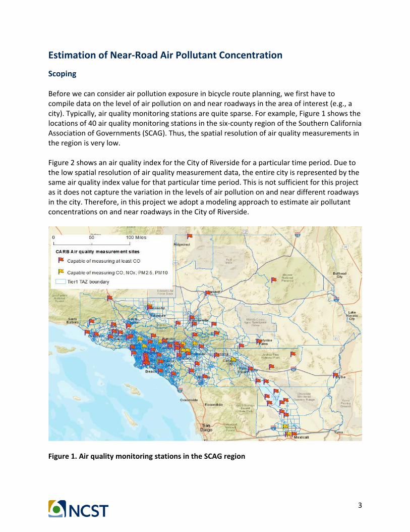
3

Estimation of Near-Road Air Pollutant Concentration

Scoping Before we can consider air pollution exposure in bicycle route planning, we first have to compile data on the level of air pollution on and near roadways in the area of interest (e.g., a city). Typically, air quality monitoring stations are quite sparse. For example, Figure 1 shows the locations of 40 air quality monitoring stations in the six-county region of the Southern California Association of Governments (SCAG). Thus, the spatial resolution of air quality measurements in the region is very low. Figure 2 shows an air quality index for the City of Riverside for a particular time period. Due to the low spatial resolution of air quality measurement data, the entire city is represented by the same air quality index value for that particular time period. This is not sufficient for this project as it does not capture the variation in the levels of air pollution on and near different roadways in the city. Therefore, in this project we adopt a modeling approach to estimate air pollutant concentrations on and near roadways in the City of Riverside.

Figure 1. Air quality monitoring stations in the SCAG region

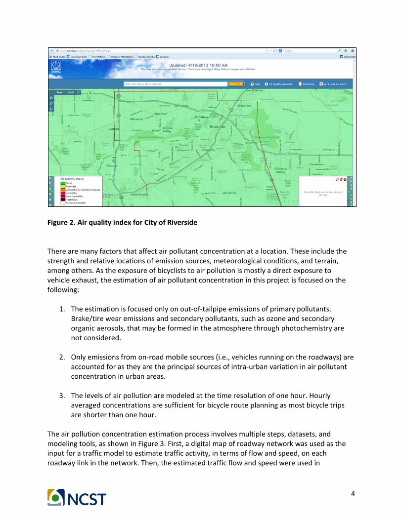
4

Figure 2. Air quality index for City of Riverside There are many factors that affect air pollutant concentration at a location. These include the strength and relative locations of emission sources, meteorological conditions, and terrain, among others. As the exposure of bicyclists to air pollution is mostly a direct exposure to vehicle exhaust, the estimation of air pollutant concentration in this project is focused on the following:

1. The estimation is focused only on out-of-tailpipe emissions of primary pollutants. Brake/tire wear emissions and secondary pollutants, such as ozone and secondary organic aerosols, that may be formed in the atmosphere through photochemistry are not considered.

2. Only emissions from on-road mobile sources (i.e., vehicles running on the roadways) are

accounted for as they are the principal sources of intra-urban variation in air pollutant concentration in urban areas.

3. The levels of air pollution are modeled at the time resolution of one hour. Hourly

averaged concentrations are sufficient for bicycle route planning as most bicycle trips are shorter than one hour.

The air pollution concentration estimation process involves multiple steps, datasets, and modeling tools, as shown in Figure 3. First, a digital map of roadway network was used as the input for a traffic model to estimate traffic activity, in terms of flow and speed, on each roadway link in the network. Then, the estimated traffic flow and speed were used in

5

conjunction with an emission model to estimate the corresponding traffic emissions on each roadway link. Finally, these emission estimates were input into a dispersion model to estimate air pollution concentration at receptor locations.

Figure 3. Traffic-related air pollution modeling process

Traffic Activity and Emissions Modeling Traffic activity data (in terms of traffic flow and speed) on roadway links in and around the City of Riverside were obtained directly from the Riverside County Transportation Analysis Model (RIVTAM), which is the regional transportation model of Riverside County, California. The data were available for four periods: morning (6-9 a.m.), midday (9 a.m.-3 p.m.), afternoon (3-7 p.m.), and nighttime (7 p.m.-6 a.m.). Traffic flow data include separate values for six vehicle types: 1) DA: passenger car driving alone; 2) SR2: passenger car shared ride with 2 persons; 3) SR3: passenger car shared ride with 3 or more persons; 4) LHDT: light-heavy duty trucks; 5) MHDT: medium-heavy duty trucks; and 6) HHDT: heavy-heavy duty trucks. Total flow is the summation of the flow values of all the six vehicle types, as shown in Figure 4. On the other hand, traffic speed data only has one value that represents the speed for all vehicle types. To estimate traffic emissions, emission factors were obtained from the California Air Resources Board’s EMFAC model version 2014 for the fleet composition in Riverside County in calendar year 2017. EMFAC is the regulatory emission model for California. As an example, fine particle (PM2.5) emission factors for speed from 5 mph to 70 mph were obtained for multiple vehicle categories in EMFAC, which were then matched with vehicle types in RIVTAM according to Table 1. After that, the total PM2.5 emission on each roadway link was calculated as:

𝐸𝐸𝑖𝑖 = ∑ 𝑞𝑞𝑖𝑖,𝑗𝑗 ∙ 𝑒𝑒(𝑣𝑣𝑖𝑖)𝑗𝑗 ∀ 𝑖𝑖𝑗𝑗 = 1, 2, 3,…, 743 Equation (1) where Ei is total emission on roadway link i (grams); qi,j is flow of vehicle type j on roadway link i (vehicles per hour); and e(vi)j is emission factor of vehicle type j for the speed on roadway link i (grams per mile). The calculation was performed for all the roadway links not only in but also around the study area, so that the effect of traffic-related air pollution carried into the study area by wind would be accounted for.

Traffic Network Traffic Activity Traffic Emissions Air Pollutant

Concentration

Traffic Model(RIVTAM)

Traffic Model(RIVTAM)

Emission Model (EMFAC2007)

Emission Model (EMFAC2007)

Dispersion Model (CALINE4)

Dispersion Model (CALINE4)

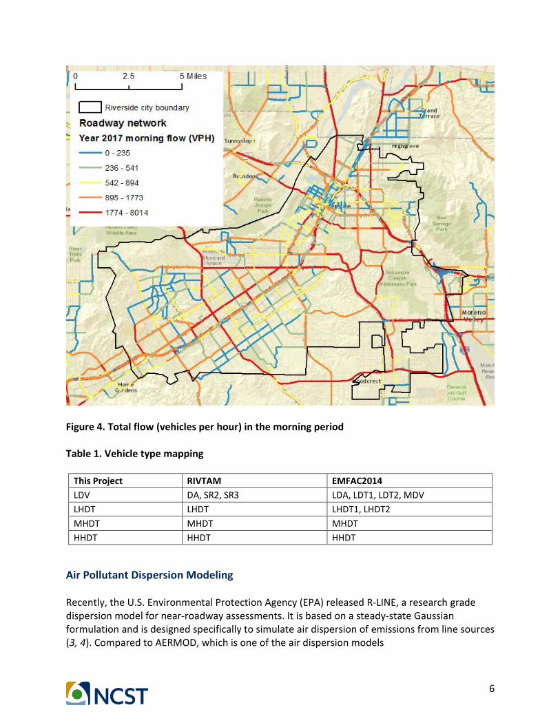
6

Figure 4. Total flow (vehicles per hour) in the morning period Table 1. Vehicle type mapping

This Project RIVTAM EMFAC2014 LDV DA, SR2, SR3 LDA, LDT1, LDT2, MDV LHDT LHDT LHDT1, LHDT2 MHDT MHDT MHDT HHDT HHDT HHDT

Air Pollutant Dispersion Modeling Recently, the U.S. Environmental Protection Agency (EPA) released R-LINE, a research grade dispersion model for near-roadway assessments. It is based on a steady-state Gaussian formulation and is designed specifically to simulate air dispersion of emissions from line sources (3, 4). Compared to AERMOD, which is one of the air dispersion models

7

preferred/recommended by the EPA and is required in modeling and analysis for regulatory purposes, R-LINE requires the same level of data inputs but computes much faster – an attribute that is important for the modeling work in this project. In addition, R-LINE has a succinct input configuration. Therefore, R-LINE was selected for use in this project. R-LINE treats traffic-related emissions as line sources. That is, roadway links are represented by lines in the model, and on each link the level of traffic emissions is evenly distributed along the lines. The underlying relationship between air pollutant concentration and the line sources in R-LINE can be expressed as:

𝑪𝑪(𝒙𝒙,𝒚𝒚, 𝒛𝒛) = 𝒇𝒇(𝑸𝑸, 𝒔𝒔𝒔𝒔𝒔𝒔𝒔𝒔𝒔𝒔𝒔𝒔 𝒍𝒍𝒔𝒔𝒔𝒔𝒍𝒍𝒍𝒍𝒍𝒍𝒔𝒔𝒍𝒍,𝒎𝒎𝒔𝒔𝒍𝒍𝒔𝒔𝒔𝒔𝒔𝒔𝒍𝒍𝒔𝒔𝒎𝒎𝒚𝒚 ) Equation (2)

where C(x,y,z) denotes emission concentration at a receptor location; and Q is average emission rate of on-road vehicles (grams/meter/second) obtained from traffic emission modeling in the previous step. For source location, each line segment’s nodes coordinates are required. Typical meteorological data for R-LINE, such as air temperature, wind speed, wind direction, surface friction velocity, Monin-Obukhov length, etc., are available from the South Coast Air Quality Management District (5). An example R-LINE input control file is illustrated in Figure 5. The blue texts mark the mandatory inputs and they should be placed at exact corresponding lines. Blue arrows point to pre-calculated attributes of geographic features (e.g., receptors, roadway links, and weather stations). Black arrows represent the use of MATLAB (6) script to select attributes and generate input control files. Pink arrows indicate that MATLAB calls R-LINE and computes receptor concentration. This schematic graph applies to the estimation of air pollutant concentration at all receptors in the model runs. In order to estimate high-resolution PM2.5 concentration at the street level, receptors were set up as a 100 m × 100 m gridded network at the height of 1.5 m. This yielded 48,000 receptors in the modeling area with more than 8,000 roadway links.

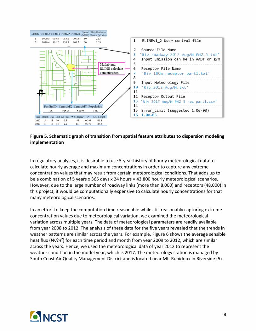
8

Figure 5. Schematic graph of transition from spatial feature attributes to dispersion modeling implementation In regulatory analyses, it is desirable to use 5-year history of hourly meteorological data to calculate hourly average and maximum concentrations in order to capture any extreme concentration values that may result from certain meteorological conditions. That adds up to be a combination of 5 years x 365 days x 24 hours = 43,800 hourly meteorological scenarios. However, due to the large number of roadway links (more than 8,000) and receptors (48,000) in this project, it would be computationally expensive to calculate hourly concentrations for that many meteorological scenarios. In an effort to keep the computation time reasonable while still reasonably capturing extreme concentration values due to meteorological variation, we examined the meteorological variation across multiple years. The data of meteorological parameters are readily available from year 2008 to 2012. The analysis of these data for the five years revealed that the trends in weather patterns are similar across the years. For example, Figure 6 shows the average sensible heat flux (W/m2) for each time period and month from year 2009 to 2012, which are similar across the years. Hence, we used the meteorological data of year 2012 to represent the weather condition in the model year, which is 2017. The meteorology station is managed by South Coast Air Quality Management District and is located near Mt. Rubidoux in Riverside (5).

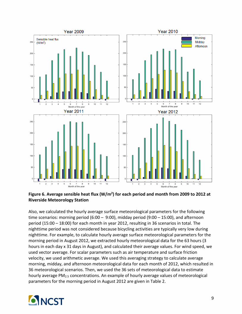
9

Figure 6. Average sensible heat flux (W/m2) for each period and month from 2009 to 2012 at Riverside Meteorology Station Also, we calculated the hourly average surface meteorological parameters for the following time scenarios: morning period (6:00 – 9:00), midday period (9:00 – 15:00), and afternoon period (15:00 – 18:00) for each month in year 2012, resulting in 36 scenarios in total. The nighttime period was not considered because bicycling activities are typically very low during nighttime. For example, to calculate hourly average surface meteorological parameters for the morning period in August 2012, we extracted hourly meteorological data for the 63 hours (3 hours in each day x 31 days in August), and calculated their average values. For wind speed, we used vector average. For scalar parameters such as air temperature and surface friction velocity, we used arithmetic average. We used this averaging strategy to calculate average morning, midday, and afternoon meteorological data for each month of 2012, which resulted in 36 meteorological scenarios. Then, we used the 36 sets of meteorological data to estimate hourly average PM2.5 concentrations. An example of hourly average values of meteorological parameters for the morning period in August 2012 are given in Table 2.

10

Table 2. Critical surface meteorological parameters and their hourly averaged values for morning period in August 2012

Parameter Value year 12 month 8 day 15 hour 6 sensible heat (W/m2) 40.34 u* - surface friction velocity (m/s) 0.11 w* - convective velocity scale (m/s) 0.7 VPTG - vertical potential temperature above Zic (K/m) 0.021 Zic - height of convectively-generated boundary layer (m) 245 Zim - height of mechanically-generated boundary layer (m) 110 L - Monin-Obukhov length (m) -100.8 Zo - surface roughness length (m) 0.314 Bo - Bowen ratio 1 Albedo 0.39 ws - reference wind speed (m/s) 0.2 wd – reference wind direction (degree) 132 zref - reference height for wind (m) 9.1 temp - reference emperature (K) 296 Ztemp - reference height for temperature (m) 5.5

During the modeling steps described above, data from different sources were extracted and computed on a link-by-link basis and parsed as binary files which could be directly manipulated by programming tools such as MATLAB. Using MATLAB scripts, model inputs including roadway geometry, emission factors, and meteorological data were written into text files and fed to the R-LINE program suite to calculate PM2.5 concentration values. Figure 7 shows a color map of PM2.5 concentrations in the City of Riverside during the morning period in August 2012, which is one of the 36 scenarios modeled in this project.

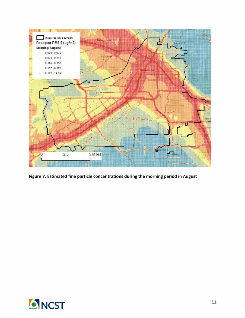
11

Figure 7. Estimated fine particle concentrations during the morning period in August

12

Generating Air Pollution Exposure Map for Bicycle Route Planning

Weighting Air Pollution Concentration Based on Bicycling Activities To use the modeled air pollution data to assist in bicycle route planning, the PM2.5 concentration values for the 36 scenarios were weighted based on the level of bicycle activities during each time scenario. For example, if more bicycle trips occur in the morning hours than during midday, a larger weight was given to the concentration values for the morning period than those for midday. The reason for using the weighting method is that bicycle facilities, once planned and built, are not likely to be easily moved. Therefore, it is reasonable to weight the PM2.5 concentration values for the different time scenarios based on the level of bicycle activities during each time scenario to result in one set of reference PM2.5 concentration values for the purpose of planning future bicycle facilities. To acquire bicycle activity data by hour of day and by month for the City of Riverside, we reviewed several travel surveys and datasets associated with bicycle use. Table 4 summarizes the data availability of selected surveys (7-9). After the review, it was clear that the GPS dataset from the California Household Travel Survey was the only source that can be used to compile hourly bicycle trip counts by month. Data from the entire State of California, instead of just a subset that fall in the boundary of the City of Riverside, were used because there are not enough bicycle trip counts within the boundary of the city to compile an hourly profile by month. Table 3. Reviewed data sources of bicycle trip counts in California

Figure 8 shows the total bicycle trip counts by period of day and by month based on the GPS dataset of the California Household Travel Survey. Note that the total number of bicycle trips in the morning are generally lower than that of midday and afternoon because the morning period includes only 3 hours, which is shorter than the midday (6 hours) and afternoon (4 hours) periods. Figure 9 shows hourly averaged bicycle trip counts by period of day and by month. It shows that the number of hourly averaged bicycle trips varies significantly by month.

Data sourceCounts of total respondents in

CA who bike after filtering travel mode

Bicycling time available?

Bicycling date available?

2009 National Household Travel Survey-Person File 87 No No

2010-2012 CA Household Travel Survey-Self reported Around 1000 No No

2010-2012 CA Household Travel Survey-GPS logging More than 2000 Yes Yes

2010-2012 SCAG Bike Count Data Clearinghouse Around 10,000 Yes

Only containobservations for 7

months out of a year

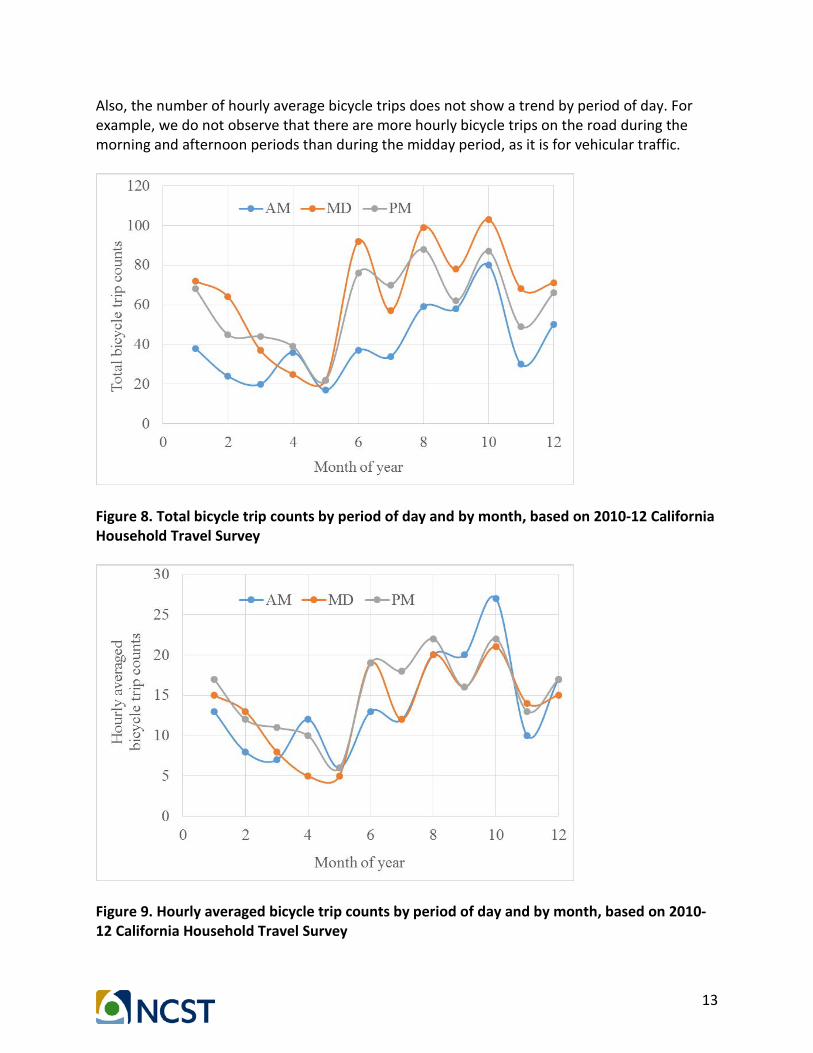
13

Also, the number of hourly average bicycle trips does not show a trend by period of day. For example, we do not observe that there are more hourly bicycle trips on the road during the morning and afternoon periods than during the midday period, as it is for vehicular traffic.

Figure 8. Total bicycle trip counts by period of day and by month, based on 2010-12 California Household Travel Survey

Figure 9. Hourly averaged bicycle trip counts by period of day and by month, based on 2010-12 California Household Travel Survey

14

Based on Figure 9, we used the hourly averaged bicycle trip counts (36 data points) as weight factors for the 36 PM2.5 concentration maps generated earlier. The concentration vector for each time period of each month can be expressed as:

𝐶𝐶𝑖𝑖𝑗𝑗𝑖𝑖 = �𝑐𝑐1𝑗𝑗𝑖𝑖𝑐𝑐2𝑗𝑗𝑗𝑗…

𝑐𝑐48000,𝑗𝑗,𝑖𝑖

� Equation (3)

where i is index for receptor (from 1 to 48,000); j is index for month (from 1 to 12); and k is index for time period (from 1 to 3, representing morning, midday and afternoon, respectively). The final concentration vector, C, can be calculated by Equation (4):

𝐶𝐶 =∑ (𝐶𝐶𝑖𝑖𝑗𝑗𝑗𝑗∙𝑐𝑐𝑜𝑜𝑜𝑜𝑜𝑜𝑜𝑜𝑗𝑗𝑗𝑗)𝑗𝑗𝑗𝑗

∑ 𝑐𝑐𝑜𝑜𝑜𝑜𝑜𝑜𝑜𝑜𝑗𝑗𝑗𝑗𝑗𝑗𝑗𝑗 Equation (4)

where 𝑐𝑐𝑐𝑐𝑐𝑐𝑐𝑐𝑐𝑐𝑗𝑗𝑖𝑖 denotes bicycle trip counts in month j and time period k, as shown in Figure 9. After weighting based on the level of bicycle activities, the final concentration map was generated as shown in Figure 10.

Figure 10. Weighted PM2.5 concentration based on bicycling activities in the State of California

15

Mapping the Exposure to Near-Road Air Pollution Concentration Using the final PM2.5 concentration map (Figure 10), a bicyclist’s exposure to traffic-related air pollution on each roadway link in the City of Riverside can be calculated. The exposure scenario in this study is a bicyclist’s direct exposure to vehicular PM2.5 in a near-road outdoor microenvironment. We use inhaled mass as a metric for quantifying the level of exposure. It is a function of air pollutant concentration that the bicyclist is exposed to, duration of the exposure, and breathing rate of the bicyclist during the time of exposure. In this study, PM2.5 concentration was estimated for each roadway link. Therefore, inhaled mass of PM2.5 for bicyclist k traveling on roadway link i can be expressed as in Equation (5), assuming that the breathing rate of the bicyclist remains the same throughout the roadway link.

𝐼𝐼𝐼𝐼𝑖𝑖,𝑖𝑖 = 𝑐𝑐𝑖𝑖 ∙ 𝑐𝑐𝑖𝑖,𝑖𝑖 ∙ 𝐵𝐵𝐵𝐵𝑖𝑖,𝑖𝑖 Equation (5) where IM is inhaled mass of PM2.5 (µg); c is PM2.5 concentration (µg/m3) along the roadway link; t is travel duration (minutes); and BR is breathing rate of the bicyclist (m3/minute). c is calculated by first extracting the locations of vertices on each link and then determining the PM2.5 concentration at each location from the concentration map. Each link has at least 3 vertices (i.e., start point, midpoint, and end point), and c is calculated as the average of the concentration values at all the vertices. The bicycling duration on a roadway link was calculated based on the link length (meters) and the assumed speed of an average bicyclist of 9 miles per hour, which is based on the real-world data in the GPS dataset of the 2010-12 California Household Travel Survey. The breathing rate of an average bicyclist is assumed to be 0.04 m3/minute based on health studies (10-12). Figure 11 shows the level of exposure to PM2.5 for an average bicyclist on a link-by-link basis, where the inhaled mass values are normalized by link length. The color map is categorized by five quantiles based on the normalized exposure values and the number of links. As expected, the map shows that most of the links in the top 20% bracket (red color) are on, or in close proximity to, the two major freeways passing through the city—State Route 91 (SR-91) and State Route 60 (SR-60). However, it is observed that for the SR-91 corridor north of Arlington Avenue the red colored links are mostly on the west side of SR-91, while they are mostly on the east side of SR-91 for the corridor south of Arlington Ave. This may be due to the different wind directions in the area in the 36 different time periods. For the SR-60 corridor, most of the red colored links are south of the freeway. For non-freeway roads, the major arterials in the city—Magnolia Boulevard, Van Buren Blvd, and Arlington Ave—also have several links that are in the top 20% bracket. This information about potential exposure of bicyclists to harmful air pollution can be used in conjunction with other information pertinent to safety, connectivity, accessibility, and other metrics in the planning of new bicycle routes and facilities.

16

Figure 11. Traffic-related primary PM2.5 exposure per mile for bicyclists

Developing an Interactive Bicycle Route Planning Tool To develop an online tool for future bicycle facility planning, we have integrated the following map layers:

1. Traffic-related PM2.5 exposure for an average bicyclist, total inhaled mass, and inhaled mass normalized by link length, as shown in Figure 5. In addition, the road network map contains other information that are relevant in bicycle facility planning such as link length, roadway speed limit category, and whether a road divider(s) exists or not.

2. Existing bicycle facility map, which includes Class I bicycle paths along city roads, and Class II bicycle lanes that are already built in the City of Riverside up to year 2012 (based on Riverside’s Bicycle Master Plan years 2007 and 2012).

3. Historical bicycle crash data in year 2014 within the City of Riverside (based on California Highway Patrol - Statewide Integrated Traffic Records System (http://iswitrs.chp.ca.gov/Reports/jsp/userLogin.jsp). The map layer labels the accident

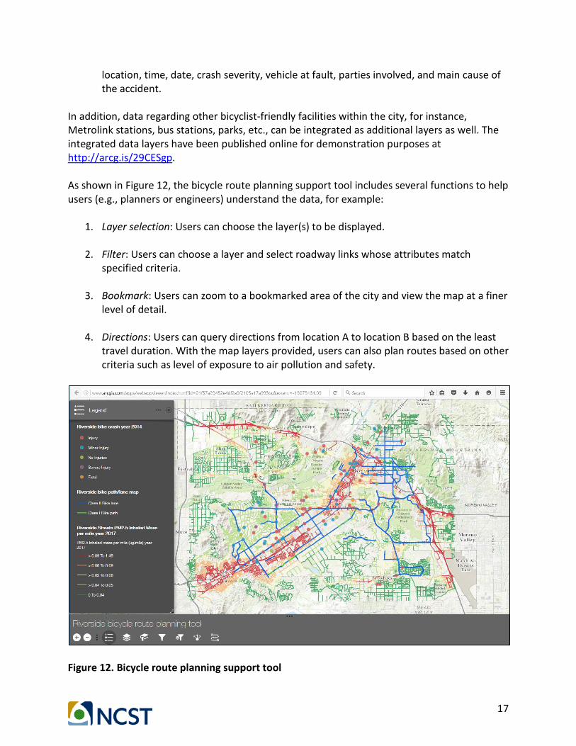
17

location, time, date, crash severity, vehicle at fault, parties involved, and main cause of the accident.

In addition, data regarding other bicyclist-friendly facilities within the city, for instance, Metrolink stations, bus stations, parks, etc., can be integrated as additional layers as well. The integrated data layers have been published online for demonstration purposes at http://arcg.is/29CESgp. As shown in Figure 12, the bicycle route planning support tool includes several functions to help users (e.g., planners or engineers) understand the data, for example:

1. Layer selection: Users can choose the layer(s) to be displayed. 2. Filter: Users can choose a layer and select roadway links whose attributes match

specified criteria.

3. Bookmark: Users can zoom to a bookmarked area of the city and view the map at a finer level of detail.

4. Directions: Users can query directions from location A to location B based on the least

travel duration. With the map layers provided, users can also plan routes based on other criteria such as level of exposure to air pollution and safety.

Figure 12. Bicycle route planning support tool

18

Case Studies of Considering Traffic-Related Air Pollution Exposure in Bicycle Route Planning According to the American Association of State Highway and Transportation Officials (AASHTO), the most important factors to be considered for bicycle planning include (13):

• User needs — Balancing the full range of needs of current and future bicyclists.

• Traffic volumes and speeds — Motor vehicle traffic volumes and speeds should be considered along with the roadway width. Some bicyclists will avoid roadways with high speeds and heavy volumes of traffic, unless they are provided with a facility that offers some degree of separation from traffic. By contrast, people who regularly use a bicycle for transportation often use main roadways because their directness and higher priority at intersections typically make them more efficient routes. In many cases, the best approach is to improve the arterial roadway to accommodate bicycles, but to also provide a parallel route along streets with lower speeds and traffic volumes.

• Overcoming barriers – Overcoming constraints and physical barriers such as freeways or

waterways should be a top priority when developing a bikeway network. A single major barrier (e.g., difficult intersection, bridge without sidewalks or bike lanes) can render an otherwise attractive bikeway corridor undesirable. Input from local bicyclists, along with a field analysis of major highway crossings, railroads, and river crossings, can help to identify major barriers.

• Connection to land uses – Bikeways should allow bicyclists to access key destinations.

They should connect to employment zones, parks, schools, shopping, restaurants, coffee and ice cream shops, sports facilities, community centers, major transit connections, and other land uses that form the fabric of a community.

• Directness of route – A bikeway should connect to desirable locations with as few detours

as possible. For example, does a bicyclist have to travel out of his or her way on a route with many turns to reach a safe freeway overpass? Multiple turns can disorient a rider and unnecessarily complicate and lengthen a trip.

• Logical route – Does the planned network make sense? A network should include facilities

that bicyclists already use, or have expressed interest in using.

• Intersections – Bikeways should be planned to allow for as few stops as possible, as bicycling efficiency is greatly reduced by stops and starts. If bicyclists are required to make frequent stops, for example, along streets with stop signs every block, they may avoid the route or disregard traffic control devices. Signalized intersections with very short green times (such as those on low-priority streets) can lead to disregard for traffic control. At

19

major streets, crossings should be carefully planned and managed to ensure maximum safety and flow.

• Aesthetics — Scenery is an important consideration along a facility, particularly for a

facility that will serve a primarily recreational purpose. Trees can also provide cooler riding conditions in summer and can provide a windbreak. Bicyclists tend to favor roads with adjacent land uses that are attractive such as campuses, shopping districts, and those with scenic views.

• Spacing or density of bikeways – A bikeway network should be planned for maximum use

and comfort, and thus should provide an appropriate density relative to local conditions. Some bicycle network plans have set a goal to provide a bicycle facility within one-fourth of a mile of every resident.

• Overall feasibility — Decisions regarding the location of new bikeways may also include

an overall assessment of feasibility given physical or right-of-way constraints, as well as other factors that may impact the cost of the project. While funding availability may influence decisions, it is essential that a lack of funds not result in a poorly-designed or constructed facility. The decision to implement a bikeway plan should also be made with a conscious, long-term commitment to a proper level of maintenance. Facility selection should seek to maximize user benefit per dollar funded.

In this section, we use the estimated PM2.5 concentration data to demonstrate the incorporation of bicyclists’ exposure to traffic-related air pollution in the planning of two bicycle routes in the City of Riverside, California. The City last updated its Bicycle Master Plan in 2012 (14). Figure 13 shows the existing and proposed bicycle facilities in the City as of February 2012. A meeting was held with the City’s Bicycle Program Coordinator to discuss potential case studies for use in this research. Two candidate corridors were identified, as circled in Figure 13.

1. University of California at Riverside (UCR) – Downtown Riverside (DTR) corridor: This corridor connects the two major trip origins/destinations in the city with potential for having high bicycle mode share. Currently, there exist bike lanes on University Ave between UCR and a MetroLink (commuter train) station just east of the SR-91 freeway. The 2012 Bicycle Master Plan Update proposed extending the bike lanes on University Ave into the downtown area.

2. Van Buren corridor around Martin Luther King (MLK) High School: This area has a high number of bicycle-related accidents, steep road grade, and high roadway intersection density, which pose challenges to bicyclists. Currently, there exist bike lanes on Van Buren Blvd east of MLK High School. The 2012 Bicycle Master Plan Update proposed extending these bike lanes further west.

20

Figure 13. City of Riverside’s existing and proposed bicycle facilities as of February 2012 In the following subsections, we explore alternative routes for adding bicycle lanes in each of these corridors, and compare between the alternative routes based on several criteria including bicyclists’ exposure to PM2.5.

UC Riverside - Downtown Riverside Corridor Figure 14 shows the detail of the UC Riverside – Downtown Riverside corridor. Since there are already some bicycle facilities along this corridor—notably on part of University Ave, Linden Street, and 3rd St—we conduct a comparison for a short segment on each route, illustrated by the three pairs of dots in Figure 14. The blue, red, and magenta dots represent the start and end of the alternative route segments on University Ave, Mission Inn Ave, and 3rd St, respectively. The dots east of SR-91 are on Park Ave where the existing bike lanes on University Ave end. The dots west of SR-91 are on Main St where the existing bike lanes on 3rd St end. The segments on these three alternative routes are chosen in a way that they have a similar length. Information regarding attributes of each route segment are obtained through a combination of the regional transportation model, digital maps, street images, and site visits. Figure 15 shows

UCR

DTR

MLK High School

21

an example street image on each of the three alternative route segments. Then, Table 4 lists key attributes of each route segment that are related to the factors that should be considered when planning bicycle routes. Some of the attribute values are qualitative, therefore when comparing the attribute values among the three alternatives, it is appropriate to use an ordinal scale or rank order (1st, 2nd, 3rd, …).

Figure 14. Alternative bicycle routes between UCR and Downtown Riverside Table 5 shows the ranking of the three alternative route segments. For each attribute, such as posted speed limit, the three alternative route segments are ranked from 1 to 3, where 1 is the best and 3 is the worst. As an example, for the posted speed limit, Mission Inn Ave is ranked 1 as it has the lowest posted speed limit (25 mph) while University Ave is ranked 3 as it has the highest posted speed limit (35 mph). For some attributes, the ranking may be tied. For example, in the case of terrain and road grade both 3rd St and Mission Inn Ave are both level in general, whereas University Ave has uphill and downhill around the SR-91 overpass. In this case, University Ave is ranked 3 and the other two routes share the rank of 1.5. Similarly, in the case of barriers where both 3rd St and Mission Inn Ave have train tracks while University Ave does not, University Ave is ranked 1 and the other two routes share the rank of 2.5, which is the average of 2 and 3. Also given in Table 5 is the weight of importance of each attribute. The weight is also based on an ordinal scale from 1 to 10, with a higher weight being more important.

Downtown Riverside

University Ave

3rd St

Linden St

UC Riverside

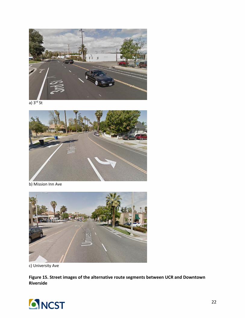
22

a) 3rd St

b) Mission Inn Ave

c) University Ave Figure 15. Street images of the alternative route segments between UCR and Downtown Riverside

23

Table 4. Attributes of alternative route segments between UCR and Downtown Riverside

Attributes 3rd St Mission Inn Ave University Ave Connection to land uses Mix of residential and

industry, few people on street

Mix of residential and businesses, many people on street

Mostly businesses, moderate number of people on street

Posted speed limit (mph) 30 25 35 Total number of lanes 3 2 4 Road shoulder width (ft) 5 5 5 Estimated average daily traffic volume in year 2017 (vehicles/lane/day)

5,577 9,455 5,628

Terrain and road grade Generally level Generally level Uphill and downhill around SR-91 bridge

Roadside parking allowed? Most sections do not allow parking

Most sections allow parking

Most sections do not allow parking

Barriers Train tracks Train tracks None Number of intersections along the segment

8 8 6

Total PM2.5 exposure (µg) 0.09 0.11 0.14 Table 5. Ranking of alternative route segments between UCR and Downtown Riverside (lower value is better)

Attributes Weight of Importance

3rd St Mission Inn Ave

University Ave

Connection to land uses 10 3 1 2 Posted speed limit (mph) 9 2 1 3 Total number of lanes 8 2 3 1 Road shoulder width (ft) 7 2 2 2 Estimated average daily traffic volume in year 2017 (vehicles/ln/day)

6 1.5 3 1.5

Terrain and road grade 5 1.5 1.5 3 Roadside parking allowed? 4 1.5 3 1.5 Barriers 3 2.5 2.5 1 Number of intersections along the segment

2 2.5 2.5 1

Total PM2.5 exposure (µg) 1 1 2 3 Simple average rank 1.95 2.15 1.90 Weighted average rank 2.07 1.98 1.95

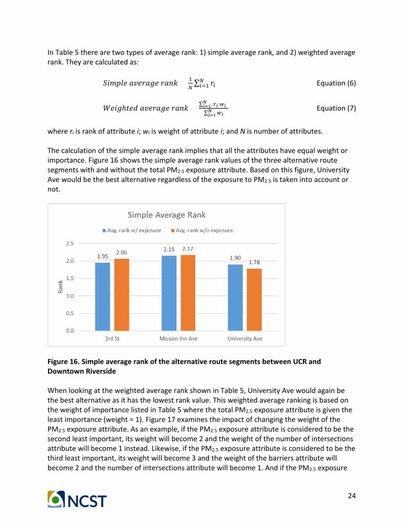
24

In Table 5 there are two types of average rank: 1) simple average rank, and 2) weighted average rank. They are calculated as:

𝑆𝑆𝑖𝑖𝑆𝑆𝑆𝑆𝑆𝑆𝑒𝑒 𝑎𝑎𝑣𝑣𝑒𝑒𝑎𝑎𝑎𝑎𝑎𝑎𝑒𝑒 𝑎𝑎𝑎𝑎𝑐𝑐𝑟𝑟 = 1𝑁𝑁∑ 𝑎𝑎𝑖𝑖𝑁𝑁𝑖𝑖=1 Equation (6)

𝑊𝑊𝑒𝑒𝑖𝑖𝑎𝑎ℎ𝑐𝑐𝑒𝑒𝑡𝑡 𝑎𝑎𝑣𝑣𝑒𝑒𝑎𝑎𝑎𝑎𝑎𝑎𝑒𝑒 𝑎𝑎𝑎𝑎𝑐𝑐𝑟𝑟 = ∑ (𝑟𝑟𝑖𝑖∙𝑤𝑤𝑖𝑖)𝑁𝑁𝑖𝑖=1∑ 𝑤𝑤𝑖𝑖𝑁𝑁𝑖𝑖=1

Equation (7)

where ri is rank of attribute i; wi is weight of attribute i; and N is number of attributes. The calculation of the simple average rank implies that all the attributes have equal weight or importance. Figure 16 shows the simple average rank values of the three alternative route segments with and without the total PM2.5 exposure attribute. Based on this figure, University Ave would be the best alternative regardless of the exposure to PM2.5 is taken into account or not.

Figure 16. Simple average rank of the alternative route segments between UCR and Downtown Riverside When looking at the weighted average rank shown in Table 5, University Ave would again be the best alternative as it has the lowest rank value. This weighted average ranking is based on the weight of importance listed in Table 5 where the total PM2.5 exposure attribute is given the least importance (weight = 1). Figure 17 examines the impact of changing the weight of the PM2.5 exposure attribute. As an example, if the PM2.5 exposure attribute is considered to be the second least important, its weight will become 2 and the weight of the number of intersections attribute will become 1 instead. Likewise, if the PM2.5 exposure attribute is considered to be the third least important, its weight will become 3 and the weight of the barriers attribute will become 2 and the number of intersections attribute will become 1. And if the PM2.5 exposure

25

attribute is considered to be the most important, its weight will become 10 and the weight of all the other attributes will be lowered by one accordingly.

Figure 17. Weighted average rank of the alternative route segments between UCR and Downtown Riverside

Based on Figure 17, University Ave would be the best alternative if the weight of the PM2.5 exposure attribute is 1, as in Table 5. However, Mission Inn Ave would become the best alternative if the weight of the PM2.5 exposure attribute is between 2 and 9. If the weight of the PM2.5 exposure attribute is 10, then 3rd St would become the best alternative. As indicated earlier and shown in Figure 14, there are already bike lanes on 3rd St, which are part of the gridded bicycle facility network of the city. 3rd St is included in this case study for comparison purposes only. On the other hand, there are no existing bike lanes on either University Ave or Mission Inn Ave, and the two streets are just a block away from each other. Both streets offer connection to another major area where Mission Inn Ave extends further west across Santa Ana River into the City of Rubidoux, while University Ave extends into the east side of the City of Riverside to UCR. Both will be a natural alternative for forming part of the gridded bicycle facility network of the city. Therefore, they are truly competing alternatives for building bike lanes. Based on the information in Table 4, both streets have pros and cons. The results in Figure 17 indicate that either street would be a suitable candidate depending on whether exposure to traffic-related air pollution is taken into consideration and how important this factor is relative to other factors. Figure 16 and Figure 17 illustrate an example of how the consideration of exposure to traffic-related air pollution could impact the outcome of bicycle route planning. It is noted that the bicycle route planning process may vary from one city to another, and planners/engineers in different cities may elect to use the information about exposure to traffic-related air pollution differently. For instance, both the order and the weight of importance for the different

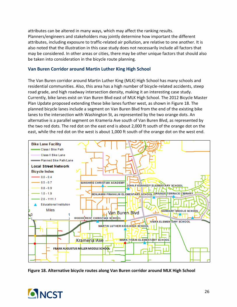
26

attributes can be altered in many ways, which may affect the ranking results. Planners/engineers and stakeholders may jointly determine how important the different attributes, including exposure to traffic-related air pollution, are relative to one another. It is also noted that the illustration in this case study does not necessarily include all factors that may be considered. In other areas or cities, there may be other unique factors that should also be taken into consideration in the bicycle route planning.

Van Buren Corridor around Martin Luther King High School The Van Buren corridor around Martin Luther King (MLK) High School has many schools and residential communities. Also, this area has a high number of bicycle-related accidents, steep road grade, and high roadway intersection density, making it an interesting case study. Currently, bike lanes exist on Van Buren Blvd east of MLK High School. The 2012 Bicycle Master Plan Update proposed extending these bike lanes further west, as shown in Figure 18. The planned bicycle lanes include a segment on Van Buren Blvd from the end of the existing bike lanes to the intersection with Washington St, as represented by the two orange dots. An alternative is a parallel segment on Krameria Ave south of Van Buren Blvd, as represented by the two red dots. The red dot on the east end is about 2,000 ft south of the orange dot on the east, while the red dot on the west is about 1,000 ft south of the orange dot on the west end.

Figure 18. Alternative bicycle routes along Van Buren corridor around MLK High School

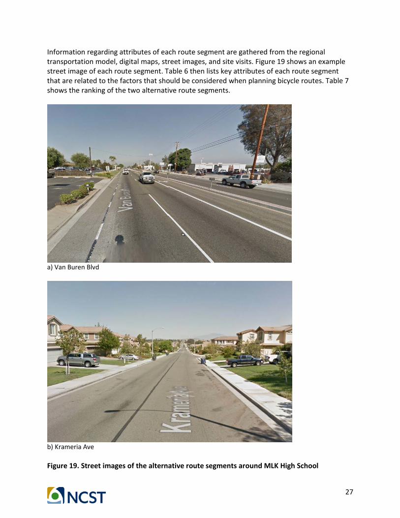
27

Information regarding attributes of each route segment are gathered from the regional transportation model, digital maps, street images, and site visits. Figure 19 shows an example street image of each route segment. Table 6 then lists key attributes of each route segment that are related to the factors that should be considered when planning bicycle routes. Table 7 shows the ranking of the two alternative route segments.

a) Van Buren Blvd

b) Krameria Ave Figure 19. Street images of the alternative route segments around MLK High School

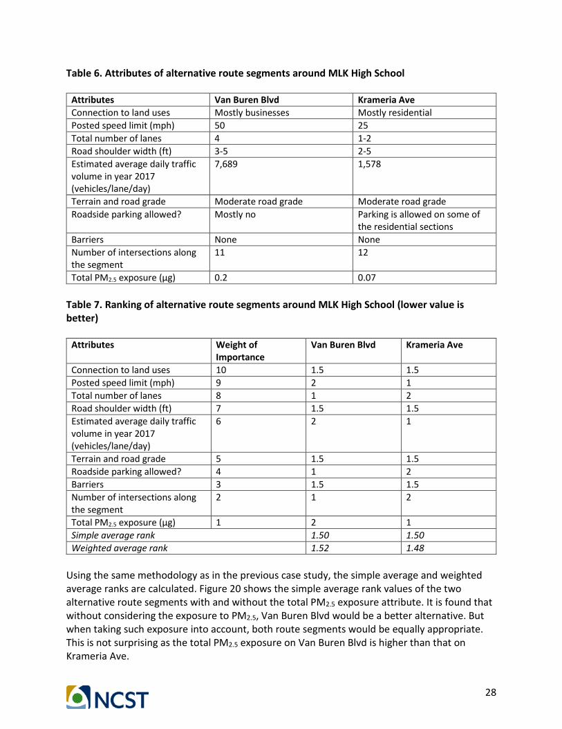
28

Table 6. Attributes of alternative route segments around MLK High School

Attributes Van Buren Blvd Krameria Ave Connection to land uses Mostly businesses Mostly residential Posted speed limit (mph) 50 25 Total number of lanes 4 1-2 Road shoulder width (ft) 3-5 2-5 Estimated average daily traffic volume in year 2017 (vehicles/lane/day)

7,689 1,578

Terrain and road grade Moderate road grade Moderate road grade Roadside parking allowed? Mostly no Parking is allowed on some of

the residential sections Barriers None None Number of intersections along the segment

11 12

Total PM2.5 exposure (µg) 0.2 0.07 Table 7. Ranking of alternative route segments around MLK High School (lower value is better)

Attributes Weight of

Importance Van Buren Blvd Krameria Ave

Connection to land uses 10 1.5 1.5 Posted speed limit (mph) 9 2 1 Total number of lanes 8 1 2 Road shoulder width (ft) 7 1.5 1.5 Estimated average daily traffic volume in year 2017 (vehicles/lane/day)

6 2 1

Terrain and road grade 5 1.5 1.5 Roadside parking allowed? 4 1 2 Barriers 3 1.5 1.5 Number of intersections along the segment

2 1 2

Total PM2.5 exposure (µg) 1 2 1 Simple average rank 1.50 1.50 Weighted average rank 1.52 1.48

Using the same methodology as in the previous case study, the simple average and weighted average ranks are calculated. Figure 20 shows the simple average rank values of the two alternative route segments with and without the total PM2.5 exposure attribute. It is found that without considering the exposure to PM2.5, Van Buren Blvd would be a better alternative. But when taking such exposure into account, both route segments would be equally appropriate. This is not surprising as the total PM2.5 exposure on Van Buren Blvd is higher than that on Krameria Ave.

29

Figure 20. Simple average rank of the alternative route segments around MLK High School According to the weighted average rank in Table 7, Krameria Ave would be a better alternative by a slight margin when the total PM2.5 exposure attribute is the least important factor (weight = 1). Figure 21 shows the impact of increasing the weight of the PM2.5 exposure attribute. According to this figure, Krameria Ave would always be the better alternative no matter how much weight is given to the PM2.5 exposure attribute, as long as it is taken into consideration. The higher the weight is the bigger the margin between Krameria Ave and Van Buren Blvd. This is due to Krameria Ave having a lower PM2.5 exposure than Van Buren Blvd.

Figure 21. Weighted average rank of the alternative route segments around MLK High School

1.2

1.3

1.4

1.5

1.6

1.7

1.8

1 2 3 4 5 6 7 8 9 10

Rank

Weight of Air Pollution Exposure Metric (10 = Most Important)

Weighted Average RankVan Buren Blvd Krameria Ave

30

When looking at the two alternative route segments in Figure 18 from the bicycle facility network perspective, they are not directly competing with each other. Van Buren Blvd would be a more natural fit for expanding the bicycle facility network in the city as it is a major arterial with many businesses. Bicyclists who want to access the amenities on Van Buren Blvd or want to travel to destinations west of the end of the existing bike lanes could benefit from extended bike lanes on this route. However, there are many schools south of Van Buren Blvd, including Woodcrest Christian School, MLK High School, Mark Twain Elementary School, and Frank Augustus Miller Middle School. For children attending these schools, Krameria Ave would be a safer and lower air pollution exposure route for them to bike to school. Adding bike lanes on this route could potentially encourage residents, especially school-aged children and their parents, to ride bicycles more. Thus, in this case study, adding bike lanes on both routes would be ideal where the bike lanes on each route would serve different types of users making different types of trip.

31

Concluding Remarks Active transportation modes such as walking and biking are key elements of sustainable transportation systems. In order to promote biking as an alternative form of transportation, a holistic approach to improving the quality of biking experience is needed. The planning of bicycle routes typically takes into consideration available right-of-way, existing roadway infrastructure, vehicular traffic volume, safety concerns, and built environment, among others. Exposure to traffic-related air pollution, on the other hand, is rarely considered despite bicyclists being vulnerable to the harmful air pollution due to their direct exposure to vehicular exhaust and increased breathing rate during biking. This research attempts to fill this gap by developing a method to incorporate reduced exposure to traffic-related air pollution as another consideration in the bicycle route planning process in order to improve the quality of the biking experience and promote active travel. Current air quality measurement data are not available at the spatial resolution necessary for the planning of bicycle routes. In this research, high-resolution traffic-related air pollution concentrations were estimated through a modeling process that involves traffic activity, traffic emission, and air pollutant dispersion modeling. The modeling process was applied to estimate traffic-related primary fine particle (PM2.5) concentrations in the City of Riverside, California, for traffic volumes in calendar year 2017 based on a total of 36 hourly average meteorological conditions consisting of three time periods of day (morning, midday, and afternoon) for the 12 months in calendar year 2012. The 36 sets of estimated PM2.5 concentration values were then weighted by the level of bicycle activities by time period of day and by month of year derived from the GPS dataset in the 2010-12 California Household Travel Survey. This resulted in a weighted average PM2.5 concentration map for the city, based on which the level of exposure to PM2.5 for bicyclists was estimated for each roadway link in the city. Two case studies in the City of Riverside were used to demonstrate the consideration of traffic-related air pollution exposure in bicycle route planning. In each case study, alternative routes along the same travel corridor were analyzed with respect to 10 factors including connection to land uses, posted speed limit, total number of lanes, road shoulder width, traffic volume, terrain and road grade, roadside parking, presence of barriers, number of intersections, and total PM2.5 exposure. As some of these factors are qualitative, the comparison between the alternative routes was made by rank order. The use of equal, as well as different, weight of importance for each factor was evaluated. In terms of exposure to traffic-related air pollution, the comparison results reveal that the best alternative route depends on whether this factor is taken into consideration and how important this factor is relative to other factors. This research has developed a method for incorporating exposure to traffic-related air pollution as another consideration in the bicycle route planning process and has demonstrated how to apply the method through two case studies. Planners and engineers may elect to adopt the presented method or use the information about exposure to traffic-related air pollution differently. For instance, both the order and the weight of importance for the different factors

32

can be changed, which may affect the ranking results. Planners/engineers and stakeholders may jointly determine how important the different factors, including exposure to traffic-related air pollution, are in relation to one another. Other factors that should be taken into consideration for a specific corridor or area may also be included. Several aspects of this research can be improved and expanded in the future, for instance, including other sources of emissions and background concentration. Also, the biking speed and breathing rate assumptions can be refined by using values specific to demographic groups such as school-aged children and by accounting for waiting time at crossings and intersections. And if air quality measurement data become available at the necessary spatial resolution, they can be used in lieu of the estimated values in the bicycle route planning process directly.

33

References

1. Woodcock, J., Edwards, P., Tonne, C., Armstrong, B.G., Ashiru, O., Banister, D., Beevers, S., Chalabi, Z., Chowdhury, Z., Cohen, A., 2009. Public health benefits of strategies to reduce greenhouse-gas emissions: urban land transport. The Lancet, 374(9705), 1930-1943.

2. Maizlish, N., Woodcock, J., Co, S., Ostro, B., Fanai, A., Fairley, D., 2013. Health cobenefits and transportation-related reductions in greenhouse gas emissions in the San Francisco Bay area. American Journal of Public Health, 103(4), 703-709.

3. Community Modeling & Analysis System, R-LINE. https://www.cmascenter.org/r-line/. 4. Snyder, M. and H. David. User Guide for R-LINE Model 1.2. USEPA/ORD/NERLMD-81.

Atmospheric Exposure Research Branch, Atmospheric Modeling and Analysis Division, Research Triangle Park, NC, 2013

5. South Coast Air Quality Management District, Meteorological Data for AERMOD. http://www.aqmd.gov/home/library/air-quality-data-studies/meteorological-data/data-for-aermod.

6. MathWorks, Matlab: The language of technical computing. http://www.mathworks.com/products/matlab/.

7. National Household Travel Survey, 2009 National Household Travel Survey. http://nhts.ornl.gov/download.shtml

8. National Renewable Energy Laboratory, 2010-2012 California Household Travel Survey Transportation Secure Data Center. http://www.nrel.gov/transportation/secure_transportation_data.html

9. Southern California Association of Governments, 2010-2012 SCAG Bike Count Data Clearinghouse. http://www.bikecounts.luskin.ucla.edu/Download_Data.aspx.

10. Adams, W. Measurement of breathing rate and volume in routinely performed daily activities, Final report. Prepared for the California Air Resources Board, Contract, No. A033-205. Human Performance Laboratory, Physical Education Department, University of California, Davis, 1993. http://www.arb.ca.gov/research/single-project.php?row_id=64931.

11. Lucía, A., Carvajal, A., Calderón, F.J., Alfonso, A., Chicharro, J.L., 1999. Breathing pattern in highly competitive cyclists during incremental exercise. European journal of applied physiology and occupational physiology 79 (6), 512-521.

12. Pankow, J., Figliozzi, M., and Bigazzi, A., 2014. Evaluation of Bicyclists Exposure to Traffic-Related Air Pollution along Distinct Facility Types. NITC-RR-560. Portland, OR: Transportation Research and Education Center (TREC). http://dx.doi.org/10.15760/trec.121

13. American Association of State Highway and Transportation Officials (2012), AASHTO Guide for the Development of Bicycle Facilities, 4th Edition.

14. City of Riverside (2012). City of Riverside Bicycle Master Plan Update, March.