STATE GDP DEFLATOR AND STATE PI - C G A Cap Commission... · PRICE AND QUANTITY INDICES NOMINAL vs....

STATE GDP DEFLATOR AND

STATE PI PRESENTED TO:

Connecticut Spending-Cap Commission

Legislative Office Building-Hartford

July 18, 2016

Daniel W. Kennedy, Ph.D.

Adjunct Faculty-Economics Department

University of Connecticut

Former Senior Economist (Retired)

Office of Research

Connecticut Department of Labor

STATE GDP DEFLATOR AND

STATE PI

I. PRICE AND QUANTITY INDICES

II. STATE GDP

III. STATE PI

I. PRICE AND QUANTITY

INDICES

PRICE AND QUANTITY

INDICES • Price Index- A price

index expresses the cost

of a market basket of

goods relative to its cost

in some “base” period,

which is simply the year

used as a basis of

comparison. [Baumol and

Blinder (2010), p. 127]

Quantity index-A

Quantity index,

particularly used for GDP

by State, are Fisher

indices calculated using a

formula consisting of

combinations of prices

and quantities for the

same year, and indices of

relative prices for two

adjacent years [U.S. BEA

(2006), p. 41]

TABLE 1: Price and Quantity Indices

INDEX

PRICE INDEX Holds the Quantity constant and

allows the price to vary.

QUANTITY INDEX Holds the price constant and

allows the quantity to vary

Laspeyres

LPI= 𝚺(𝐏𝐭

𝚺(𝐏𝟎

x 𝐐𝟎)

x 𝐐𝟎)

Where:

P0 = Price in the base

period

Q0 = Quantity purchased

in the base period

Pt = Price in the current

period.

LQI= (𝚺𝐏𝟎

𝚺(𝐏𝟎

x 𝐐𝐭)

x 𝐐𝟎)

Where:

P0 = Price in the base

period


in the base period

Qt = Quantity purchased

in the current

period.

Paasche

PPI= 𝚺(𝐏𝐭

𝚺(𝐏𝟎

x 𝐐𝐭)

x 𝐐𝒕 )

Where:

P0 = Price in the previous

period

Qt = Quantity purchased

in the current period


period.

PQI= 𝚺(𝐏𝐭

𝚺(𝐏𝐭

x 𝐐𝐭)

x 𝐐𝟎)

Where:


in the previous period

Qt = Quantity purchased in

the current period


period.

Fisher’s

Ideal

Index

𝐋𝐏𝐈 x 𝐏𝐏𝐈

𝐋𝐐𝐈 x 𝐏𝐐𝐈

PRICE AND QUANTITY

INDICES NOMINAL vs. REAL, or CONSTANT-

DOLLAR GDP

Nominal GDP rises when prices rise, even if there is no

increase in actual production.

For example, if hamburgers cost $2.00 this year but cost

only $1.50 last year, then 100 hamburgers will contribute

$200 to this year’s nominal GDP, whereas they contributed

only $150 to last year’s nominal GDP.

But one hundred hamburgers are still 100 hamburgers—

output has not grown. [Baumol and Blinder (2010), p. 88]

Comparing the CPI with the GDP Price

Index and Implicit Price Deflator

CPI-U vs. the GDP Price Index [U.S. BLS, Comparing

the Consumer Price Index with the gross domestic product price

index and gross domestic product implicit price deflator, MLR

(March 2016)]

The GDP Price Index, like the CPI, measures price

change for consumer goods and services, but the GDP

Price Index also measures price change for goods and

services purchased by businesses, governments, and

foreigners.

However, unlike the CPI, the GDP Price Index does not

measure price change for imports.



CPI-U vs. the GDP Price Index (Continued)

Although the GDP Price Index and the CPI both

measure changes in the prices of goods and

services purchased by consumers, the GDP relies

on the Personal Consumption Expenditures (PCE)

Price Index as its measure of change in consumer

prices.

Table 2 compares the CPI and the PCE Price

Index.

Comparing the CPI with the GDP Price Index and Implicit Price Deflator

Table 2: Comparing The CPI and The PCE Price Index

PCE Price Index CPI Produced by BEA using BLS price indexes and other data

sources.

Produced by BLS using surveys of consumer prices and other

data sources.

Reflects the price of expenditures made by households, including

those made on behalf of households.

Reflects the price of out-of-pocket expenditures made by

consumers.

Composition of expenditures changes from quarter to quarter. Composition of the market basket remains fixed (updated every

two years).

Derived using a chained Fisher index formula. Derived using a Laspeyres-type index formula.

Weights are derived from business surveys. Weights are derived from household surveys.

SOURCE: Moyer, Brian C., U.S. BEA, Comparing Price Measures—The CPI and the PCE Price Index (March 13-14, 2006) NABE

Conference



The Implicit Price Deflator [U.S. BLS (March

2016), p. 5]

The GDP Implicit Price Deflator deflates the current

nominal-dollar value of GDP by the chained-dollar value

of GDP.

The chained-dollar value is derived by updating a base-

period dollar value amount by the change in the GDP

Quantity Index, which in turn is derived with the use of a

Fisher ideal index formula that aggregates from

component GDP quantity indices.



Deriving The Implicit Price Deflator (ibid)

Once the component quantity indices are calculated, the GDP

Quantity Index can be derived and the GDP Implicit Price

Deflator is then calculated by dividing Nominal GDP by Real

GDP.

The change in the GDP Implicit Price Deflator is roughly equal

to the change in the GDP Price Index.

In fact, the GDP Implicit Price Deflator has risen at a

systematically lower annual rate than the CPI-U over time (2%

for the GDP Price Index and Implicit Price Deflator, vs. 2.4% for

the CPI-U).



Deriving Real GDP and The Implicit Price

Deflator

TABLE 3: Deriving Real GDP and The Implicit Price Deflator

Real GDP = IPD =

Year CTGDP CTQIndex Qindx/100 Base Yr X Q GDP/RGDP

2009 226,076 100.00 1.0000 226,076 100.00

2010 230,357 100.95 1.0095 228,212 100.94

2011 232,271 100.20 1.0020 226,535 102.53

2012 238,322 100.45 1.0045 227,084 104.95

2013 242,417 100.06 1.0006 226,209 107.16

2014 250,764 101.26 1.0126 228,927 109.54

SOURCE: U.S. BEA and Author's calculations

II. STATE GDP

STATE GDP: Three Sides of GDP (Based on Coyle, 2014; Table 1, p. 26)

OUTPUT (Production, or Value Added)

Gross Output (Gross Sales -- ∆Inventories)

---- Intermediate Inputs

= VALUE ADDED

INCOME (By Type)

Compensation

+ Rental Income

+ Profits + Proprietors’ Income

+ (Taxes on Production + Imports) –Subsidies

+ Interest + Miscellaneous Payments

+ Depreciation

= TOTAL DOMESTIC INCOME EARNED

FINAL DEMAND (Expenditures)

Consumer Spending (Households)

+ Investment in Plant, Equip., Software (Business)

+ Government Purchases (Goods and Services)

+ Net Exports (=Exports – Imports)

= FINAL SALES OF DOMESTIC PRODUCT

= =

Three sides to GDP: OUTPUT = INCOME = SPENDING

STATE GDP

Measuring GDP by State [U.S. BEA, Gross Domestic

Product by State Estimation Methodology (2006), p. ii]

GDP by State cannot be measured by adding the number of

goods and services produced by the states’ economies because

GDP by state consists of a variety of goods and services.

The GDP by state dollar value is necessarily measured by either

the amount of expenditures on it, or by the amount of incomes

earned by the factors of production in producing it.

GDP by state, like Gross Domestic Income (GDI) for the nation,

is measured as the factor incomes earned and the costs of

production. This is illustrated in Figure 1.

FIGURE 1: Components of State GDP

+ + = STATE GDP LABOR INCOME

Wages & Salaries

Other Benefits

Earned by Workers

BUSINESS TAXES

Federal Excise Taxes

Sales Taxes

Property Taxes

Other taxes that can

be included as a

Business Expense.

CAPITAL INCOME

Income earned by

Individual or joint

Business

Entrepreneurs as well

as Corporations.

Depreciation and

Other Income earned

by Capital.

SOURCE: U.S. BEA (2006), p. ii

STATE GDP

Real GDP by State and Chain-Weighted Quantity Indices [U.S. BEA, Gross Domestic Product by State Estimation Methodology

(2006), p. 15]

The U.S. BEA prepares chain-type quantity indices, by

industry, for the nation, but state-level information on prices

by industry is not available, so estimates of Real State GDP

are derived by applying national-level industry Implicit Price

Deflators to the Current-Dollar State GDP estimates for the

detailed industries.

Real State GDP for the aggregate industries (such as Total

Services, Manufacturing, etc.) is derived by using the same

chain-type index formula that is used in the national accounts.

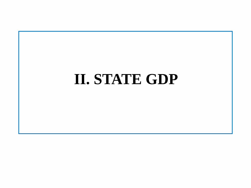
STATE GDP

To the extent that a state’s output is produced and

sold in national markets at relatively uniform prices

(or sold locally at national prices), Real State GDP

captures the relative differences in the mix of goods

and services that states produce.

However, Real State GDP does not capture state-to-

state differences in the prices of goods and services

that are produced and sold locally (i.e., Non-Tradable

Goods).

STATE GDP

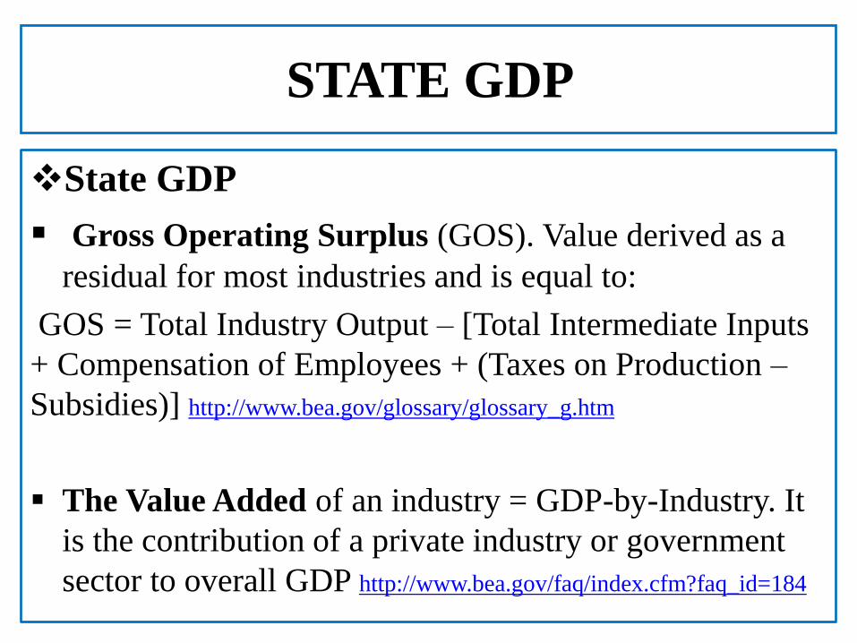
State GDP

Gross Operating Surplus (GOS). Value derived as a

residual for most industries and is equal to:

GOS = Total Industry Output – [Total Intermediate Inputs

+ Compensation of Employees + (Taxes on Production –

Subsidies)] http://www.bea.gov/glossary/glossary_g.htm

The Value Added of an industry = GDP-by-Industry. It

is the contribution of a private industry or government

sector to overall GDP http://www.bea.gov/faq/index.cfm?faq_id=184

http://www.bea.gov/glossary/glossary_g.htm

http://www.bea.gov/faq/index.cfm?faq_id=184

STATE GDP

STATE GDP: State and local government [U.S.

BEA (2006), pp. 13-14]

Gross Operating Surplus (GOS) includes:

GOS = Consumption of Fixed Capital (CFC) + Proprietors’ Income

+ Corporate Profits + Nontax Payments + Business Current Transfer

Payments (net).

The GOS estimates for State and Local Government consist of

the surplus/deficit of 16 state and local government enterprises.

The CFC for these enterprises, and state and local general

government CFC.

STATE GDP

STATE GDP: State and local government

In general, state and local government revenues less

expenditures, for each enterprise and state, from the

Census Bureau are used to distribute to the states the

national surplus or deficit of each state and local

government enterprise.

STATE GDP

STATE GDP: State and local government The CFC for state and local government (general government

and government enterprises) is distributed to the states based

on each state’s share of state and local government

employment.

Finally, the components estimated above for state and local

government—the surplus or deficit of state and local

government enterprises, the CFC for state and local

government enterprises, and the CFC for state and local

general government—are summed yielding the GOS for state

and local government.

STATE GDP

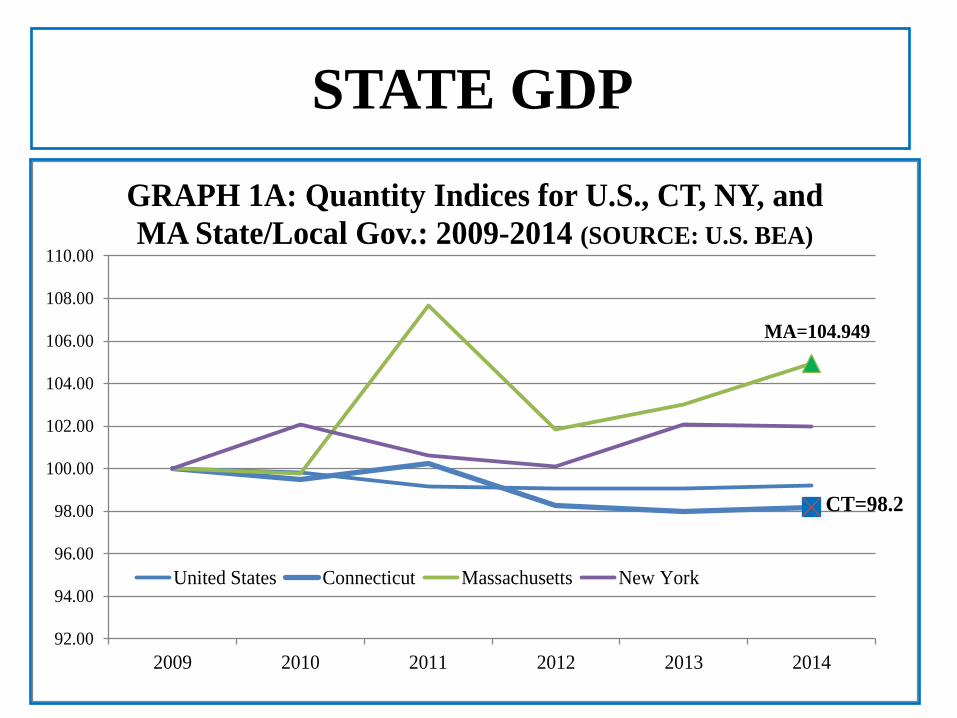
CT=98.2

MA=104.949

92.00

94.00

96.00

98.00

100.00

102.00

104.00

106.00

108.00

110.00

2009 2010 2011 2012 2013 2014

GRAPH 1A: Quantity Indices for U.S., CT, NY, and

MA State/Local Gov.: 2009-2014 (SOURCE: U.S. BEA)

United States Connecticut Massachusetts New York

STATE GDP

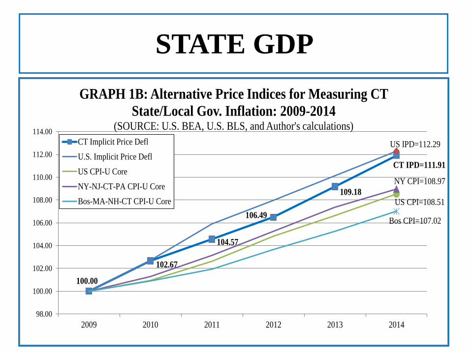
100.00

102.67

104.57

106.49

109.18

CT IPD=111.91

US IPD=112.29

US CPI=108.51

NY CPI=108.97

Bos CPI=107.02

98.00

100.00

102.00

104.00

106.00

108.00

110.00

112.00

114.00

2009 2010 2011 2012 2013 2014

GRAPH 1B: Alternative Price Indices for Measuring CT

State/Local Gov. Inflation: 2009-2014 (SOURCE: U.S. BEA, U.S. BLS, and Author's calculations)

CT Implicit Price Defl

U.S. Implicit Price Defl

US CPI-U Core

NY-NJ-CT-PA CPI-U Core

Bos-MA-NH-CT CPI-U Core

III. STATE PI

STATE PI

STATE PI vs. STATE GDP

TABLE 4: The Relation of State GDP and State and PI, 2003

State GDP State PI

Compensation of Employees 6,268.70 6,271.50

Taxes on Production and Imports 798.1 ------

LESS: Subsidies 46.7 ------

Gross Operating Surplus (GOS) 3,903.80 ------

- Proprietors’ Income ------ 839.1

EQUALS: Earnings by Place of Work ------ 7,110.60

LESS: Contributions for Government Social Insurance ------ 771.5

PLUS: Adjustment for Residence ------ –1.2

PLUS: Dividends, interest, and rent 1,475.40

PLUS: Personal current transfer receipts 1,335.30

TOTAL 10,923.80 9,148.70

SOURCE: U.S. BEA, Gross Domestic Product by State Estimation Methodology (2006), p. 1

STATE PI

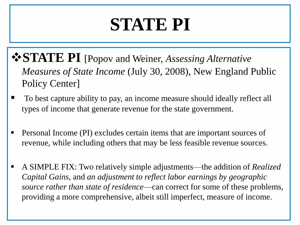
STATE PI [Popov and Weiner, Assessing Alternative

Measures of State Income (July 30, 2008), New England Public

Policy Center]

To best capture ability to pay, an income measure should ideally reflect all

types of income that generate revenue for the state government.

Personal Income (PI) excludes certain items that are important sources of

revenue, while including others that may be less feasible revenue sources.

A SIMPLE FIX: Two relatively simple adjustments—the addition of Realized

Capital Gains, and an adjustment to reflect labor earnings by geographic

source rather than state of residence—can correct for some of these problems,

providing a more comprehensive, albeit still imperfect, measure of income.

STATE PI

STATE PI (ibid)

Alternatives to the U.S. Bureau of Economic Analysis’s

(BEA) measures of income do exist.

They include:

-- The Internal Revenue Service’s (IRS) Adjusted Gross

Income (AGI)

-- The U.S. Census Bureau’s Money Income

These tend to carry even greater limitations than BEA’s PI in

either completeness or availability.

STATE PI

STATE PI (ibid)

On the other hand, two production-based measures—

the BEA’s State GDP (see Part II of this

presentation), and the U.S. Treasury Department’s

Total Taxable Resources (TTR)—are worth

considering as proxies for a state’s ability to pay.

However, they have limitations related to their

comprehensiveness, transparency, and availability.

STATE PI

STATE PI (ibid)

Perhaps the most widely used practical

measure of income is the U.S. BEA’s State

Personal Income (PI).

State PI is defined as the “income received by

persons from participation in production, from

government and business transfer payments,

and from government interest.

STATE PI

STATE PI (ibid)

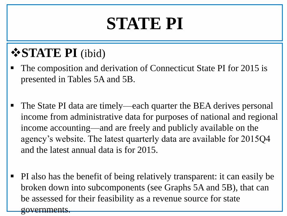
The composition and derivation of Connecticut State PI for 2015 is

presented in Tables 5A and 5B.

The State PI data are timely—each quarter the BEA derives personal

income from administrative data for purposes of national and regional

income accounting—and are freely and publicly available on the

agency’s website. The latest quarterly data are available for 2015Q4

and the latest annual data is for 2015.

PI also has the benefit of being relatively transparent: it can easily be

broken down into subcomponents (see Graphs 5A and 5B), that can

be assessed for their feasibility as a revenue source for state

governments.

STATE PI

TABLE 5A: Connecticut State PI-2015BY PLACE OF RESIDENCE

Personal income (thousands of dollars) 240,519,358

DERIVATION OF PI

Earnings by Place of Work 160,485,814

LESS: Contributions for Government Social Insurance 16,365,177

Employee and Self-Employed Contributions for Government Social Insurance 8,789,060

Employer Contributions for Government Social Insurance 7,576,118

PLUS: Adjustment for Residence 14,917,605

EQUALS: Net earnings by Place of Residence 159,038,241

PLUS: Dividends, Interest, and Rent 50,089,251

PLUS: Personal Current Transfer Receipts 31,391,866

PI PLACE OF RESIDENCE 240,519,358

SOURCE: U.S. BEA, Table SA5N

TABLE 5B: Connecticut Earnings by Place of Work-2015DERIVATION OF EARNINGS BY PLACE OF WORK

Wages and Salaries 111,425,449

Supplements to wages and salaries 25,586,190

Employer Contributions for Employee Pension and Insurance Funds 18,010,073

Employer Contributions for Government Social Insurance 7,576,118

Proprietors' Income 23,474,174

Farm Proprietors' Income 20,277

Nonfarm Proprietors' Income 23,453,897

EARNINGS BY PLACE OF WORK 160,485,813

SOURCE: U.S. BEA, Table SA5N

STATE PI

STATE PI (ibid)

Despite these advantages, there are several things to keep in mind when

using personal income to represent a state’s ability to fund programs.

Specifically, PI:

• excludes Capital Gains Income;

• captures Labor Income of state residents regardless of

where they earn it, rather than capturing all labor income

earned in the state;

• excludes Corporate Profits;

• captures contributions to pension funds rather than

disbursements;

• includes certain types of non-cash income.

STATE PI

SOURCE: Figure E, IRS, Statistics of Income Bulletin | Spring 2011, p. 177

61,089

77,624

77,789

95,920

0 20,000 40,000 60,000 80,000 100,000 120,000

All States

MA

NY

CT

2007 AGI

GRAPH 2: AGI for 2007-CT, NY, MA,

and All States

STATE PI

SOURCE: Figure C, IRS, Statistics of Income Bulletin

| Spring 2011, p. 176

18.7

20.7

23.5

25.8

0.0 5.0 10.0 15.0 20.0 25.0 30.0

All States

NY

MA

CT

2007 AGI

GRAPH 3A: % Returns with Net Capital

Gains for 2007-CT, NY, MA, and All States

33,624

41,341

53,636

60,021

0 10,000 20,000 30,000 40,000 50,000 60,000 70,000

All States

MA

CT

NY

2007 AGI

GRAPH 3B: Ave Net Capital Gain for

2007-CT, NY, MA, and All States

SOURCE: Figure C, IRS, Statistics of Income Bulletin |

Spring 2011, p. 176

Table 6: Summary of Selected Income Measures

Income Measure

Personal Income

(PI)

Adjusted Gross

Income (AGI)

CPS* Money

Income (MI) Government agency Bureau of Economic

Analysis (BEA)

Internal Revenue

Service (IRS)

U.S. Census

Bureau

Are state-level data

available?

Yes Yes Yes (Median HH

Income only)

Most recent year state

data available

Annual, 2015;

Quarterly 2015Q4

2014

2014

Are selected components included? Wages and Salaries Yes Yes Yes

Proprietors’ Income Yes Yes Yes

Dividends, Interest,

and Rent

Yes Yes (Taxable only) Yes

Employer

Pension/Insurance

Contributions

Yes No No

Pension/Retirement

Income Distributions

No Yes Yes

Government Cash

Transfers

Yes Some Yes

Government Non-

Cash Transfers

Yes No No

Interpersonal Cash

Transfers

No Some Yes

Imputed Rental

Income

Yes No No

Realized Net Capital

Gains

No Yes No

Unrealized Capital

Gains

No No No

Corporate Profits No No No

SOURCE: Table 1 Popov and Weiner (June 30, 2008) *Current Population Survey

STATE PI

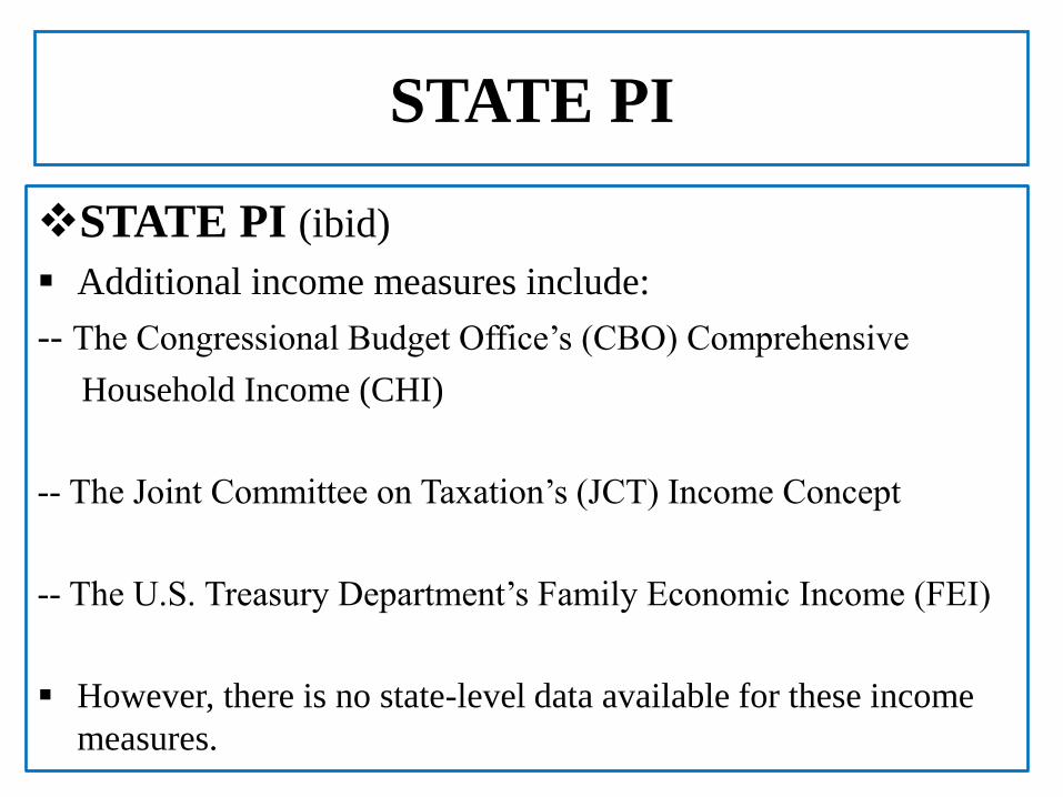
STATE PI (ibid)

Additional income measures include:

-- The Congressional Budget Office’s (CBO) Comprehensive

Household Income (CHI)

-- The Joint Committee on Taxation’s (JCT) Income Concept

-- The U.S. Treasury Department’s Family Economic Income (FEI)

However, there is no state-level data available for these income

measures.

STATE GDP DEFLATOR AND STATE PI - C G A Cap Commission... · PRICE AND QUANTITY INDICES NOMINAL vs....

Documents

Transcript of STATE GDP DEFLATOR AND STATE PI - C G A Cap Commission... · PRICE AND QUANTITY INDICES NOMINAL vs....