Stata Basics

for students in Biometry(ZOOL 631)

© Andrew D. Taylor, 2006 revised 8/20/06

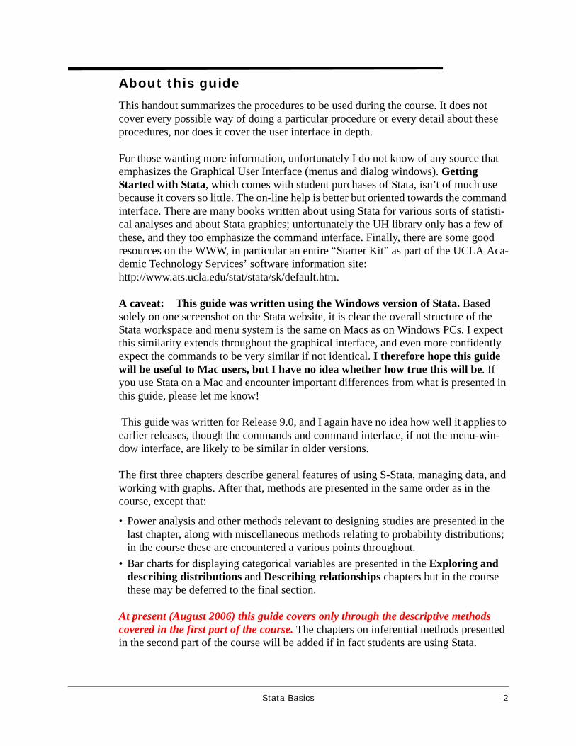
About this guide

This handout summarizes the procedures to be used during the course. It does not cover every possible way of doing a particular procedure or every detail about these procedures, nor does it cover the user interface in depth.

For those wanting more information, unfortunately I do not know of any source that emphasizes the Graphical User Interface (menus and dialog windows). Getting Started with Stata, which comes with student purchases of Stata, isn’t of much use because it covers so little. The on-line help is better but oriented towards the command interface. There are many books written about using Stata for various sorts of statisti-cal analyses and about Stata graphics; unfortunately the UH library only has a few of these, and they too emphasize the command interface. Finally, there are some good resources on the WWW, in particular an entire “Starter Kit” as part of the UCLA Aca-demic Technology Services’ software information site: http://www.ats.ucla.edu/stat/stata/sk/default.htm.

A caveat: This guide was written using the Windows version of Stata. Based solely on one screenshot on the Stata website, it is clear the overall structure of the Stata workspace and menu system is the same on Macs as on Windows PCs. I expect this similarity extends throughout the graphical interface, and even more confidently expect the commands to be very similar if not identical. I therefore hope this guide will be useful to Mac users, but I have no idea whether how true this will be. If you use Stata on a Mac and encounter important differences from what is presented in this guide, please let me know!

This guide was written for Release 9.0, and I again have no idea how well it applies to earlier releases, though the commands and command interface, if not the menu-win-dow interface, are likely to be similar in older versions.

The first three chapters describe general features of using S-Stata, managing data, and working with graphs. After that, methods are presented in the same order as in the course, except that:

• Power analysis and other methods relevant to designing studies are presented in the last chapter, along with miscellaneous methods relating to probability distributions; in the course these are encountered a various points throughout.

• Bar charts for displaying categorical variables are presented in the Exploring and describing distributions and Describing relationships chapters but in the course these may be deferred to the final section.

At present (August 2006) this guide covers only through the descriptive methods covered in the first part of the course. The chapters on inferential methods presented in the second part of the course will be added if in fact students are using Stata.

Stata Basics 2

USING STATA

Mac↔PC↔Unix Portability

Although I have not tested how perfectly it works, Stata claims that Stata data files (.dta files on Windows PCs) can be used without any translation on Macs, Windows PCs, and Unix computers. This should also apply to “do-files” (think of them as “macros”) if you use them, and hopefully applies to graphs and log files saved in Stata’s proprietary formats (.gph and SMCL, respectively). Thus you should be able to more your work seamlessly between, say, a PC at school and your iMac at home.

That said, everything further in this guide will refer to the Windows version of Stata.

The Stata workspace

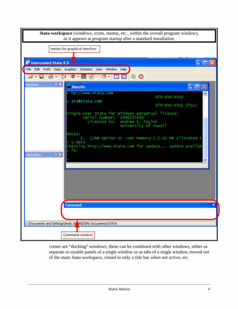
Principal windowsThe default opening appearance of Stata is shown on the next page. There are five main parts to it:

• across the top, a list of menus and, below it, a row of icons for managing and navi-gating in the workspace,

• the Command window at the bottom,• the Results window, the largest,• the Review window at upper left, which will contain the history of commands

entered or other actions taken during the current Stata session, and• the Variables menu at lower left, which will show information about the variables in

the active data set.

Other windows

Other windows that will open as called for include windows for:

• showing graphs, • viewing or editing data, • writing sequences of commands to be run as programs, and • viewing results of various procedures or actions.

Where did that window go?

All of these windows can be moved around in the Stata workspace and rearranged in a variety of ways. In particular, windows with a little stick pin in the upper-right

© Andrew D. Taylor, 2006 revised 8/20/06

corner are “docking” windows; these can be combined with other windows, either as separate re-sizable panels of a single window or as tabs of a single window, moved out of the main Stata workspace, closed to only a title bar when not active, etc.

menus for graphical interface

Command window

Stata workspace (windows, icons, menus, etc., within the overall program window),as it appears at program startup after a standard installation.

Stata Basics 4

Using Stata: Menus or commands?

Learning more about managing windows in the workspace

These behaviors of the windows and workspace can be complex and confusing; refer to Chapter 4, “The Stata user interface” of Getting Started with Stata for further explanation. Better yet, watch the short movies at

www.ats.ucla.edu/stat/stata/topics/stata9.htm under the heading “Stata Graphical User Interface,” especially the first one on “How do I make windows dock, pin, and float?”

Where’s the rest of the output?

If output is produced which is longer than the Results window can hold, display will halt after one window-full, and will be displayed at the bottom. To get the next line of output, press the Enter key. To get the next window-full, click on the —more— line or the icon, or press any key other than Enter

Menus or commands?

Stata has a menu-dialog based graphical user interface (GUI) to its procedures, oper-ated through the menus listed across the top of the overall Stata workspace (shown on the page above). Most of the statistical procedures we will need in Biometry — with the exception of the resampling methods — can be conducted through the GUI.

Stata is, however, essentially a command-driven program. It appears that the full capa-bilities of the program are accessed more effectively through the command interface and that some important capabilities for data management (as well as the resampling methods) require use of the commands for the basic analyses they are built on. Furthermore all the official and unofficial Stata documentation I have been able to find emphasizes (or even uses exclusively) the command interface. Finally, it can try one’s patience severely to wait for the dialog windows to open!

I therefore recommend learning the command interface. To help with this, in this guide I have given command equivalents to the window-menu procedures. Perhaps more usefully, almost anything you do in the Stata GUI results in the corresponding command being written in the Results window, where you can study it and learn to use the commands directly.

Stata Basics 5

Using Stata: Command-line interface

Menus and commands in this guide

In this guide, sequences of menu selections in the graphical user interface will be shown in bold arial font, with arrows showing the sequence of selections. For example, the sequence here

would be shown as

Statistics ⇒ Summaries, tables, & tests! ⇒ Classical tests of hypotheses! ⇒ Two-sample mean comparison test

Commands to be submitted in the Command window will be shown in bold courier font, for example

ttest trtmt == control, unpaired unequal welch

Command-line interface

Commands are entered in the Command window at the bottom of the overall Stata workspace, shown on the next page. Commands are typed into the window and executed by pressing the Enter key; there is no prompt symbol in the window since it isn’t used for anything else.

Command syntax

The standard syntax of Stata commands is

[prefix_cmd:] command [varlist] [if] [in] [, options]

where items in brackets are optional. The if and in items, and the most common prefix_cmd, by, are discussed in a separate section below. The other items in this standard syntax are:

• commandThe keyword for the command itself

• varlistA list of variables to be used in the command

Stata Basics 6

Using Stata: Graphical user interface (GUI)

• prefix_cmdA command modifying the application of the command, the most common being by, discussed later.

• optionsMost command have a variety of options to modify their operation, their output, etc. These must be separated from the rest of the command by a single comma; there should be no other commas in the command.

Graphical user interface (GUI)

Opening dialogs

Usually you will navigate to the dialog for a particular procedure by working through menu choices starting from the top-level Data, Graphics, or Statistics menus.

There are, though, two shortcuts which can be used to save steps or to get to a dialog when you can’t remember which menu selections to use:

• the command

db commandname

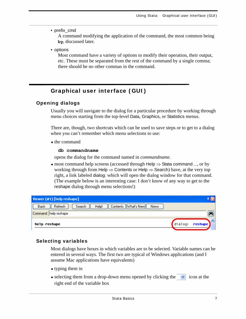
opens the dialog for the command named in commandname.• most command help screens (accessed through Help ⇒ Stata command…, or by

working through from Help ⇒ Contents or Help ⇒ Search) have, at the very top right, a link labeled dialog: which will open the dialog window for that command. (The example below is an interesting case: I don’t know of any way to get to the reshape dialog through menu selections!)

Selecting variables

Most dialogs have boxes in which variables are to be selected. Variable names can be entered in several ways. The first two are typical of Windows applications (and I assume Mac applications have equivalents)

• typing them in

• selecting them from a drop-down menu opened by clicking the icon at the right end of the variable box

Stata Basics 7

Using Stata: Saving, exporting, and printing results

Another method, I think unique to Stata, uses the Variables window: when the active cursor is in the box for variable selection in a dialog, move the mouse to the Variables window and clicking (once) on a variable in the list there will select that variable in the open dialog.

Submitting dialogs

Dialog windows in Stata have OK, Cancel, and Submit buttons at their lower left. The Cancel, as expected, exits that dialog without doing anything. OK submits the dialog and then closes its window; Submit submits the dialog and leaves it open.

Dialog settings

Entries and selections made in a dialog window are remembered when that window is opened by the next invocation of the procedure. This can be convenient in that it allows the procedure to be repeated, perhaps with some modifications, without every entry and selection having to be repeated. It also could cause problems, though, if you forget to reset selections you no longer want. To alleviate this latter problem, the dialog windows all have an icon at their bottom left which will Restore the dialog to its default settings.

Saving, exporting, and printing results

Log files

Statistical results in the Results window are lost when you exit Stata. To save them for viewing in a later Stata session, or for exporting or printing (see below), Stata uses what it calls “logs.” Once a log is begun, everything that goes into the Results window — commands and error messages as well as results — also goes into the log. The log can, though, be suspended (e.g. until you figure out how to get a command to work properly) and then re-opened. Similarly, one log can be closed and another opened, for instance to separate output from different projects.

Opening the log

• Click the Begin Log button ,• Select File ⇒ Log ⇒ Begin… and specify the file (including changing the file type

from Formatted Log to Log; see below on exporting results), or• Submit the command log using filename

If you specify an existing file to be the filename, you will be given a choice between appending the new log to the file, replacing the file, or simply opening the file for viewing (but not recording the log).

Stata Basics 8

Using Stata: Saving, exporting, and printing results

Closing the log

The log is closed automatically when you exit Stata. To close it before exiting Stata:

• Click the Begin Log button and then select Close log file,• Select File ⇒ Log ⇒ Close, • Submit the command log close.

A closed file can be re-opened by the methods above for opening a log, and specifying the existing file.

Suspending the log

If you want to temporarily stop recording results to the log, but will want to re-open it during the same Stata session, suspending it is a little easier than closing it. To suspend the log:

• Click the Begin Log button and then select Suspend log file,• Select File ⇒ Log ⇒ Suspend, • Submit the command log off.

If the log has been suspended, when you use either the Begin Log button or the File ⇒ Log selection, you will be given a choice between resuming the suspended log or closing it (or simply viewing it). The command to resume a suspended log is log on.

Viewing a log

An open or suspended log can be opened in a Stata viewer by:

• Clicking the Begin Log button and then select View snapshot of log file, or• Selecting File ⇒ Log ⇒ View… and then selecting the desired file.

Apparently only the latter method works to open a closed log for viewing, and appar-ently log files cannot be opened for viewing from the command line.

Exporting results

Log file import

The native format for Stata log files is called SMCL (Stata Markup and Control Language), which only Stata can read. This file format retains the text formatting seen in the Results window. A log file in the SMCL format cannot be read by any other application.

Alternatively, when a log file is created you can choose to have it be an unformatted text (ASCII) file, which retains the spacing in the Results window but no other format-

Stata Basics 9

Using Stata: Saving, exporting, and printing results

ting. In addition, log files in SMCL format can be translated to unformatted text format using

File ⇒ Log ⇒ Translate…and then specifying the existing file to translate, and a file to put the translated version in. The command for this is

translate “existingfile.smcl” “destinationfile.log” , replace linesize(n) translator(smcl2log)

where existingfile is the filename (with path if needed) of the log file to be trans-lated, destinationfile is the filename (with path if needed) of the file to be cre-ated, and n is the line width (default is 79).

A log file in this unformatted “.log” format can be read by any text editor or word-processor. Warning: Tabular output will be distorted by proportionally spaced fonts. To maintain proper alignment, change to a fixed-space font such as Courier.

Copy and paste

Text can be selected in either the Results window or the log viewer, then copied and pasted into a document open in another application (e.g. MS Word). The pasted text will be unformatted ASCII text; the warning above about proportionally spaced fonts applies.

Printing results

The entire contents of the Results window or of a log open in a viewer can printed. Use the GUI selections

File ⇒ Print!!!! ⇒ Resultsor

File ⇒ Print!!!! ⇒ Viewer (#n) [view …]

Printing apparently cannot be done from the command line.

Printing as exportingSince the Windows (and hopefully also the Mac OS) print dialog gives the option of sending the print job to a file rather than a printer, this gives an indirect way to export results (i.e. the Results window or a log open in a viewer) into a file format such as PostScript that retains formatting but conceivable could be opened and even edited in a different application.

Stata Basics 10

DATA ORGANIZATION, MANIPULATION, AND IMPORT/EXPORT

Data files

The Open command ( icon) works only for files already in Stata’s own format.

Stata data sets are stored in files with the .dta filename extension. Data files are orga-nized into observations (rows) and variables (columns), similar to other statistics pro-grams and somewhat like spreadsheet programs such as MS Excel.

Variables

Variable names

Default names for the variables (columns) are var1, var2, etc., but they can be renamed. Naming is much less flexible than in Minitab: variable names can include only letters, numbers, and underscores (‘_’); neither spaces or special characters are allowed. Note also that names are case-sensitive.

Variable labelsThe restrictions on variable names can be overcome by associating labels with vari-ables. There appear to be few if any restrictions on these labels. Variables can be labeled in several ways:

• Variable Properties dialogThis dialog is opened by double-clicking within a column in the Data Editor (see below); simply enter the label in the Label: box of the dialog.

• Data ⇒ Labels ⇒ Label variableThen give the variable name and label in the dialog window.

• label var varname “label”In this command varname is the name of the variable and label (which appar-ently must by enclosed in quotes) is the text of the label.

Value labels

As will be seen in the next section, Stata’s capabilities for importing data files are somewhat limited, and in particular character (= string) variables can be imported only in some kinds of files. A way around this is to replace such a variable with numeric codes, e.g. “female” = 1, “male” = 2, “juvenile” = 3. The file, now containing only numbers, now can be read into Stata. Stata will consider the variable containing the codes to be numerical, but it still can be treated as categorical.

Stata Basics 11

Data organization, manipulation, and import/export: Data files

To ease interpretation of such variables (especially, to prevent confusion about the coding scheme), the different values of such a variable — or any other numerical vari-able — can be assigned “value labels.” This can be done in several ways, paralleling those for labeling variables:

• Variable Properties dialogOpen this dialog by double-clicking within a column in the Data Editor (see below), then click on the Define/Modify button below the Value label: box of the dialog window and fill out the Define value labels dialog window that opens.

• Data ⇒ Labels ⇒ Label valuesThis actually is a two-step process. Data ⇒ Labels ⇒ Label values ⇒ Define or modify value labels

opens a dialog in which a named set of values and corresponding labels is created.

Data ⇒ Labels ⇒ Label values ⇒ Assign value labels to variableopens a dialog in which a named set of labels is assigned to a variable.

• The following pair of commands (corresponding to the preceding two menu opera-tions):label define labelset value label value label …

In this command labelset is the name of the set of codes being defined, and value and label are pairs to be associated. Then use

label values varname labelset

where varname is the variable the values are to be applied to, and labelset is the name of the labeling scheme to be applied.

Entering and importing data

Creating a new (empty) data set

Unlike other programs, Stata apparently can only have one data set open (in memory) at once. To create a data set therefore requires that you first get the current one out of memory. To do this, submit the command

clear

to empty the active data set (you may want to save it first). Then use the methods dis-cussed below to enter data.

Entering data into the open data set

Data can be entered directly into the active data set from the keyboard or by cut-and-paste from some other applications; this seems to work well from Excel. Open the Data Editor as described below (“Editing or browsing data” on page 16). Then do the usual typing and editing operations in the window.

Stata Basics 12

Data organization, manipulation, and import/export: Data files

Importing a text file

How to import a text file depends on how its columns are separated, how strings are represented, and whether variable (column) names are presented.

Delimited filesThe two easiest kinds of files to import are “delimited files”:

• Files with columns separated by tabs or commas, with or without strings and/or col-umn names.Spreadsheet programs typically create this sort of file when using the Save as text option. Some programs include variable (column) names in these files, which Stata will recognize and use. Text data files on the textbook’s CD (or website) are in this format.

• Files with columns separated by single spaces, with no column names and with string variables (if any) either as single words or enclosed in quotes.

Read in either of these types of files using

File ⇒ Import!!!!⇒ ASCII data created by a spreadsheetand selecting the file; default settings should work. Or use the command

insheet using filename

where filename is the name of the file to be imported (if the filename extension is .raw you do not need to include it; otherwise you do).

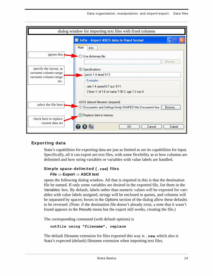
Fixed format filesAnother file format that is reasonably easy to import is one with only numerical data in fixed columns, with missing values represented by blanks or periods, and with no col-umn names. Text data files I distribute for this course will be in this format, with any string variables represented by numerical codes. Read in such files using

File ⇒ Import!!!!⇒ ASCII data in fixed formatwhich opens the dialog below:

The same task can be accomplished using the command

infix varname1 columnrange1 … using filename

where ‘varname1 columnrange1 …’ is a sequence of variable names and column ranges (exactly as in the Specifications box of the dialog window above), and file-name is the name of the file to be imported (if the filename extension is .raw you do not need to include it; otherwise you do).

Importing from other applications

Unfortunately Stata cannot directly import files saved by other applications (e.g. Excel) in their own formats. The only two ways to import data from other applications are by cut-and-paste (from data open in the other application) or by saving a text file from the other application.

Stata Basics 13

Data organization, manipulation, and import/export: Data files

Exporting data

Stata’s capabilities for exporting data are just as limited as are its capabilities for input. Specifically, all it can export are text files, with some flexibility as to how columns are delimited and how string variables or variables with value labels are handled.

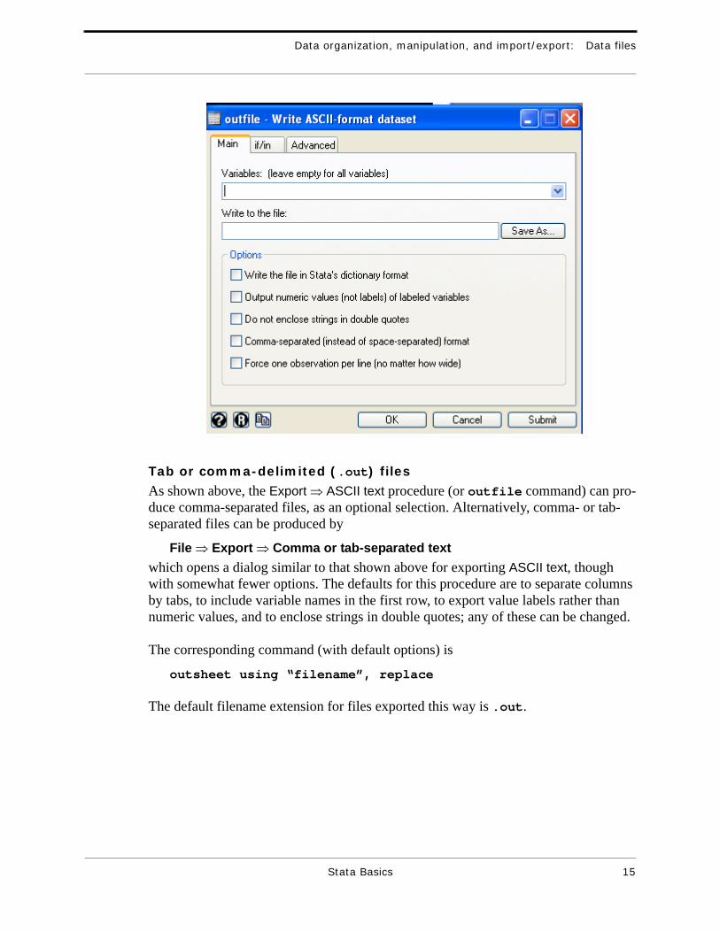
Simple space-delimited (.raw) filesFile ⇒ Export ⇒ ASCII text

opens the following dialog window. All that is required in this is that the destination file be named. If only some variables are desired in the exported file, list them in the Variables: box. By default, labels rather than numeric values will be exported for vari-ables with value labels assigned, strings will be enclosed in quotes, and columns will be separated by spaces; boxes in the Options section of the dialog allow these defaults to be reversed. (Note: if the destination file doesn’t already exist, a note that it wasn’t found appears in the Results menu but the export still works, creating the file.)

The corresponding command (with default options) is

outfile using “filename”, replace

The default filename extension for files exported this way is .raw, which also is Stata’s expected (default) filename extension when importing text files.

dialog window for importing text files with fixed columns

select the file here

check here to replacecurrent data set

ignore this

specify the layout, asvarname column-rangevarname column-range

etc.

Stata Basics 14

Data organization, manipulation, and import/export: Data files

Tab or comma-delimited (.out) files

As shown above, the Export ⇒ ASCII text procedure (or outfile command) can pro-duce comma-separated files, as an optional selection. Alternatively, comma- or tab-separated files can be produced by

File ⇒ Export ⇒ Comma or tab-separated textwhich opens a dialog similar to that shown above for exporting ASCII text, though with somewhat fewer options. The defaults for this procedure are to separate columns by tabs, to include variable names in the first row, to export value labels rather than numeric values, and to enclose strings in double quotes; any of these can be changed.

The corresponding command (with default options) is

outsheet using “filename”, replace

The default filename extension for files exported this way is .out.

Stata Basics 15

Data organization, manipulation, and import/export: Data set manipulation

Data set manipulation

Editing or browsing data

The current data set can be edited in the usual ways (typing new values, deleting col-umns or rows, cut-and-paste to move data around, etc.) in the Data Editor. This can be opened by any of the following routes:

• the icon• Data ⇒ Data editor• Window ⇒ Data Editor• ctrl+7 (i.e. hold down the ctrl key and type 7)• the command edit

If you only way to examine the data, however, without making any changes, a safer way is through the Data Browser. It is opened by analogs of some of the ways of opening the Data Editor:

• the icon• Data ⇒ Data browser (read-only editor)• the command browse

Intermediate between these two, it is possible to open data in the Data Editor allowing only designated parts of the data set to be changed; see the section on edit with in and if in Chapter 8, Using the Data Editor, of Getting Started with Stata.

If, in and by processing

Controlling which observations are used in a command, and how, seems to be a focal part of Stata’s design: the if and in methods for this are distinct elements in standard command syntax, as is the prefix_cmd which usually is a by command, and most

The remainder of this section is still being written.

Stata Basics 16

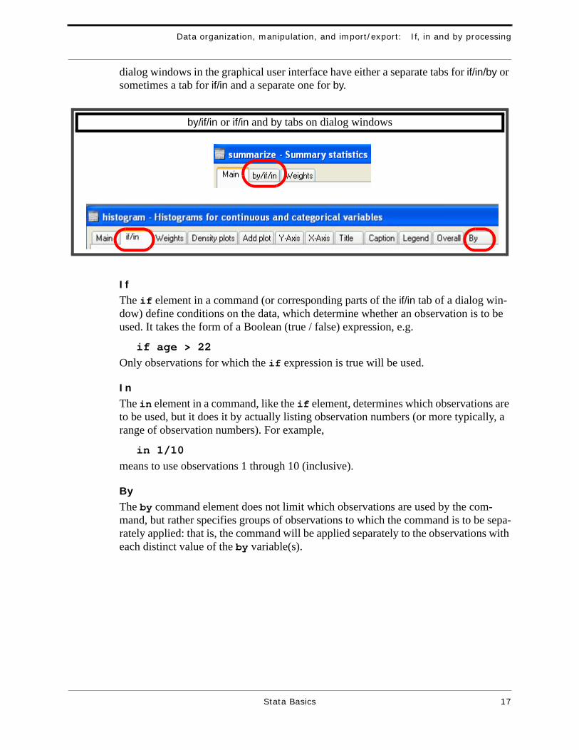
Data organization, manipulation, and import/export: If, in and by processing

dialog windows in the graphical user interface have either a separate tabs for if/in/by or sometimes a tab for if/in and a separate one for by.

If

The if element in a command (or corresponding parts of the if/in tab of a dialog win-dow) define conditions on the data, which determine whether an observation is to be used. It takes the form of a Boolean (true / false) expression, e.g.

if age > 22

Only observations for which the if expression is true will be used.

In

The in element in a command, like the if element, determines which observations are to be used, but it does it by actually listing observation numbers (or more typically, a range of observation numbers). For example,

in 1/10

means to use observations 1 through 10 (inclusive).

By

The by command element does not limit which observations are used by the com-mand, but rather specifies groups of observations to which the command is to be sepa-rately applied: that is, the command will be applied separately to the observations with each distinct value of the by variable(s).

by/if/in or if/in and by tabs on dialog windows

Stata Basics 17

STATA GRAPHING: GENERAL FEATURES

Stata appears to have very good graphing capabilities, but I have far too little experi-ence with the program to know for sure how well this works. In this chapter I describe some general aspects of creating and working with Stata graphs; details for specific sorts of graphs are presented in the appropriate later chapters.

Creating graphs

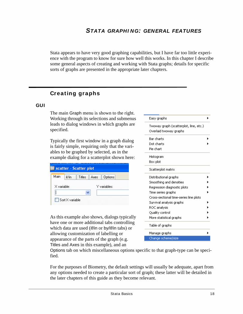
GUI

The main Graph menu is shown to the right. Working through its selections and submenus leads to dialog windows in which graphs are specified.

Typically the first window in a graph dialog is fairly simple, requiring only that the vari-ables to be graphed by selected, as in the example dialog for a scatterplot shown here:

As this example also shows, dialogs typically have one or more additional tabs controlling which data are used (if/in or by/if/in tabs) or allowing customization of labelling or appearance of the parts of the graph (e.g. Titles and Axes in this example), and an Options tab on which miscellaneous options specific to that graph-type can be speci-fied.

For the purposes of Biometry, the default settings will usually be adequate, apart from any options needed to create a particular sort of graph; these latter will be detailed in the later chapters of this guide as they become relevant.

Stata Basics 18

Commands

In a sense most graphs are subtypes of a generic graph command, as for example the command for a simple scatterplot, which can be given in full as

graph scatter mpg weight

or, since scatter implies it is a graphing command, in shortened form asscatter mpg weight

The by, if and in command elements can be used with most of not all graph commands. Some of the fundamental aspects of graph type and appearance are deter-mined as part of the basic command (e.g. in the scatterplot example here, the basic command really is graph scatter), while others are controlled by options (given after the basic command and variable specification, following a comma).

Multiple graphs

How to make multiple related graphs, e.g. the same graph for different groups of data, depends on the data layout and whether the graphs are to be overlaid, put in separate panels, or (for some graph types) shown side-by-side in one graph.

‘Overlaid twoway graphs’ procedures

These procedures are the most flexible way to create overlaid graphs, but their default settings do not do as well at distinguishing the separate graphs as does the simple method for “unstacked” data described below, so typically the appearance options need to be carefully controlled.

The basic menu selection is

Graphics ⇒ Overlaid twoway graphsThe dialog window (shown below) has many tabs: four for the (up to four) plots to be overlaid plus the usual tabs for controlling axes (including an optional second vertical axis) and other aspects of graph appearance.

Each of the Plot tabs has a long list of possible plot types; many of these are not rele-vant for this course, but the first few are, as is the last item on the list, Histogram. Once a plot type is selected, the other parts of the Plot tab will change to those appropriate for that type. It is here that default choices of, e.g. symbol type, size and color in a scatterplot, may need to be overridden to make a legible overlaid graph.

The corresponding command depends greatly on what the plot types are. The basic syntax is

twoway (plotspecification1) (plotspecification2) …

where plotspecificationn is a command, variable selection, and all other con-trols or desired options appropriate to the plot type. For a very simple example,

twoway (scatter Y1 X1) (scatter Y2 X2)

will overlay two scatterplots, of Y1 vs. X1 and Y2 vs. X2.

Stata Basics 19

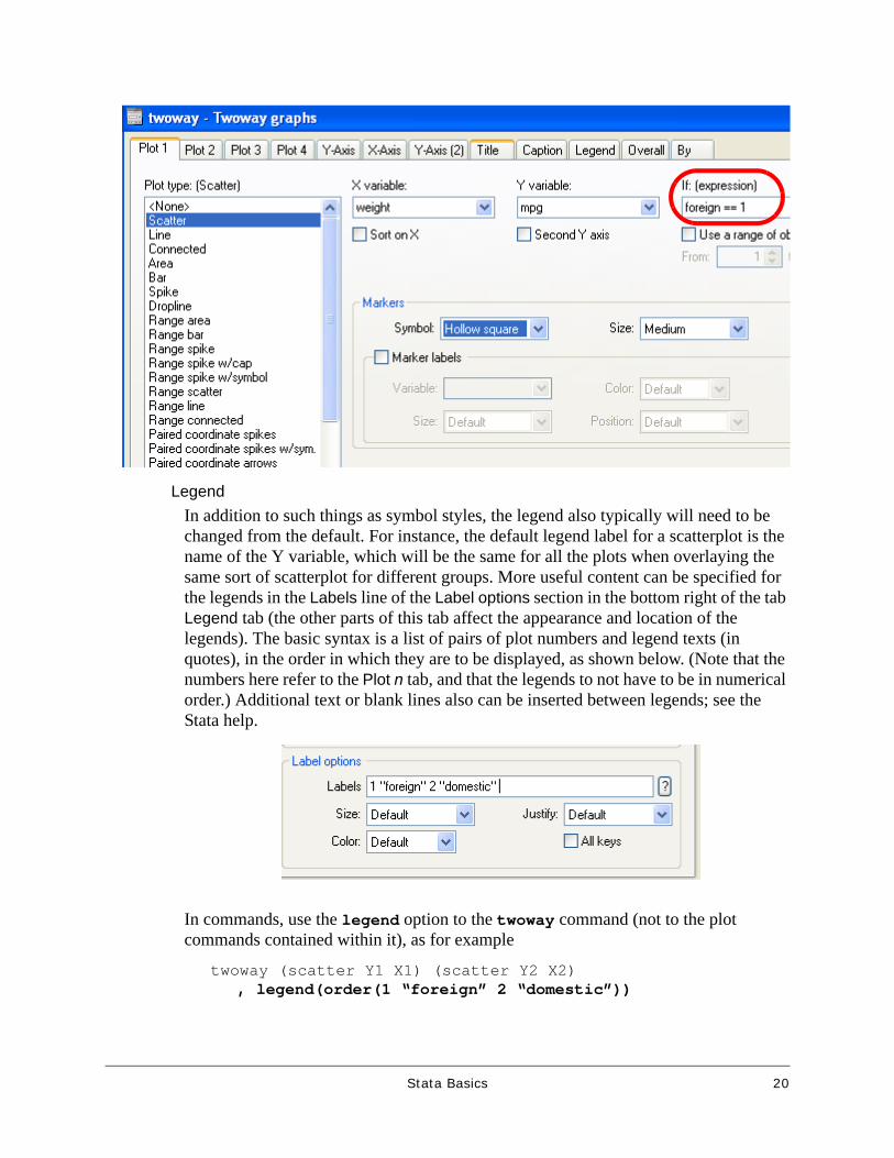
LegendIn addition to such things as symbol styles, the legend also typically will need to be changed from the default. For instance, the default legend label for a scatterplot is the name of the Y variable, which will be the same for all the plots when overlaying the same sort of scatterplot for different groups. More useful content can be specified for the legends in the Labels line of the Label options section in the bottom right of the tab Legend tab (the other parts of this tab affect the appearance and location of the legends). The basic syntax is a list of pairs of plot numbers and legend texts (in quotes), in the order in which they are to be displayed, as shown below. (Note that the numbers here refer to the Plot n tab, and that the legends to not have to be in numerical order.) Additional text or blank lines also can be inserted between legends; see the Stata help.

In commands, use the legend option to the twoway command (not to the plot commands contained within it), as for example

twoway (scatter Y1 X1) (scatter Y2 X2) , legend(order(1 “foreign” 2 “domestic”))

Stata Basics 20

Unstacked dataIf the data are “unstacked” (data for the different plots, or at least the Y variables for scatterplots, in different columns) using this Overlaid twoway graphs procedure is simple: the different sets of columns are specified on the different Plot tabs.

Stacked dataIf, though, the different plots are to be of different parts of the same columns, the procedure is less straightforward. In this situation, the different plots should not be distinguished by a By variable; doing so would put them on different panels of the graph, rather than overlaid.

Instead, each plot must be restricted to the desired subset of observations using If conditions. This is illustrated in the circled part of the dialog shown on the previous page. In commands, the if condition is put just before any options to the commands for the particular plot; for example:

twoway (scatter mpg weight if foreign == 1, options)(scatter mpg weight if foreign != 1, options)

Remember that, as noted above, the appearance of points, lines, etc., for the different plots will need to be modified so that they can be distinguished.

Combining two graph commands

An alternative to using the Overlaid twoway graphs method just described, in which several plots are specified within the overall twoway command, is to join to graph commands by the special || operator. (The | symbol is typed as shift-\) It typically will be necessary to control the symbols, lines, etc., so that they differ between the two graphs. Thus an equivalent to the command in the previous paragraph would be

scatter mpg weight if foreign == 1 , options || scatter mpg weight if foreign !=1 , options

I do not think this method can be used through the GUI.

Other overlaid graphs

The only other way I know of to overlay graphs works only if the data for the different graphs are in separate columns. In this situation overlaid graphs are straightforward for most plot types: simply list the several variables in the part of the dialog or command in which the plot variable(s) is specified.

Exactly how this will work will depend on the plot type. For instance, for scatterplots only one X variable can be listed and if multiple Y variables are specified the plots will be overlaid (with different symbols), while for boxplots the plots for all the listed variables will be side-by-side rather than overlaid (but still will use the same axis scaling).

Stata Basics 21

Paneled graphs

As far as I can tell, the only way to put multiple plots using data from different sets of columns in different panels of the same graph is to first make the separate plots, then use the Table of graphs method described below (under “Viewing multiple graphs” on page 26).

If the data for all the groups (i.e. all the intended panels of the multiple graph) are in the same column(s), with one or more group identifiers in other columns, it is very easy to have the plots as panels in a single graph window: use the identifier variable(s) as By variable(s). In the GUI, all procedures for which this is possible have a By tab in the dialog; in the command interface, by is a “prefix command.”

Graphs ‘over’ a variable

For some graph types that are essentially one dimensional — notably, box plots — the data can be subdivided “over” a grouping variable, if the data are in the “stacked” layout. Using the “over” command puts the several plots next to each other within a single axis area; in contrast, using the grouping variable in a “by” command would put the plots in separate panels of the graph window.

In the GUI, dialogs for plot types for which this method is allowed will have a tab labeled Over or Over groups. On this tab simply name the grouping variable as the Over 1 variable. (One or two additional grouping variables can be specified as the Over 2 and Over 3 variables, giving a hierarchical grouping of the data.)

The command-line equivalent is an option, e.g.

graph box mpg, over(foreign)

Graph styles

Graphs are not editable

As far as I can tell, graphs cannot be modified once they are created, except that the “scheme” used to display them (see below) can be changed. To get effects or appear-ances other than the defaults, you will need to

• use the graph options and other controls at the time you make a graph, and/or • use a different “scheme” (see below), perhaps a custom one you have created; this

can be done when the graph is made or later.

Appearance options

Options directly affecting the content of a graph, and important appearance options specific to a particular kind of graph, will be described in later chapters of this guide, as those graphs are discussed. There are some useful appearance options, however, which are general:

Stata Basics 22

• Y-axis, X-axisJust about everything about the appearance of the axes can be controlled: axis labels (content as well as font, justification, etc.), tick mark placement and appearance, axis scaling, grid lines, etc.

• title and subtitleBoth what the titles are, and their appearance, can be controlled.

• legendWhether to show a legend, what its content should be, and its appearance all can be controlled.

• the parts of the graph windowThe size and appearance of the whole graph window, the plot area within it, their borders and buffers, etc., can be controlled; these are on the Overall tab of the graph dialog.

These options all can be included in graph commands, but there are so many of them to learn, it probably will be easier to use the graphical user interface and its dialog windows whenever you want to substantially modify graph options. (If there are particular options you change often, you can learn the command-line syntax by first using the GUI dialogs and then inspecting the resulting commands in the Results window.)

Graphic “schemes”

Stata uses what it calls “schemes” to define coordinated sets of appearance options for graphs. As the Stata help files say:

There are several standard schemes included when you install Stata. These vary prima-rily in their use of colors, though there also are subtle differences in such things as the text used for labels. The default scheme is called s2color; it uses a light colored (but not white) background. Another useful scheme is s2mono, which is designed for printing on monochrome printers and uses different symbols rather than different colors to, for instance, distinguish groups in scatterplots. s1rcolor is a simple scheme in reverse color, i.e. light on a dark background, which might be useful for displaying on screen or by projector.

If you find yourself routinely overriding some defaults of graph appearance, you may want to create a modified scheme with those changes; see the Stata help for informa-tion on how to do this.

Stata Basics 23

Applying a scheme to a graph

A scheme can be specified at the time a graph is made, either as an entry on the Overall tab of the dialog in the GUI, or as the scheme option in the graph command, as for instance

graph histogram ages, scheme(s1rcolor)

A graph also can be re-displayed later using a different scheme; this seems to be as close as Stata comes to providing editing of graphs after their creation. The GUI procedure for this is

Graphics ⇒ Change scheme/sizeThis opens a simple dialog in which you choose the graph to be re-displayed and the scheme to be used; there also are options for re-sizing the graph. The corresponding command is

graph display graphname, scheme(schemename)

Setting your default scheme

In the GUI,

Prefs ⇒ Graph preferences…opens a dialog in which you change the scheme that is used by default when new graphs are made. Similarly, the command

set scheme schemename [, permanently]

sets the default scheme to schemename; the permanently option makes this perma-nent in that it is applied to all future Stata sessions (until you change it again), while if this option is not specified the change applies only for the duration of the current Stata session.

Managing graphs

Stata can have multiple graphs in memory and perhaps displayed simultaneously in the workspace, but only one, usually the most recently created one, is “current” at a time. This has some important implications which affect how you manage graphs during a Stata session.

Naming graphs

Stata names each new graph “Graph” by default. This has the unfortunate conse-quence, apparently, of causing the current graph to be replaced — and lost — when-ever a new graph is created. To prevent this, each graph that you want to keep must be given a unique name.

Graphs can be named as they are created:

Stata Basics 24

• In the GUI one of the tabs, often the Options tab or an Overall tab, will have a box in which you can specify the Name of graph (and optionally choose to have the new graph replace the existing graph of that name if there is one).

• Most if not all graph commands have a name option, with the simple syntaxname(graphname)

A graph also can be named, or renamed:

• In the GUI, byGraphics ⇒ Manage graphs!!!! ⇒ Rename graph in memory

which opens a dialog in which you select which graph to rename (remember, the current graph, if you didn’t yet name it, is named “Graph”) and its new name.

• With the simple commandgraph rename oldname newname

Other basic graph management

In addition to (re)naming graphs, you can copy them, drop them from memory, switch which one is “current,” and get descriptive information on them.

Copy

This presumably would be useful if you want to modify a graph (as discussed above under Editing Graphs) while keeping the original version as well.

Graphics ⇒ Manage graphs!!!! ⇒ Copy graph in memoryopens a dialog in which you select which graph (“current” or a named graph in memory) to copy, and give a name for the new graph.graph copy existinggraph copyname

Drop

to clear graphs from memory.Graphics ⇒ Manage graphs!!!! ⇒ Drop graphsgraph drop graphname(s)

Switch which is current

Graphics ⇒ Manage graphs!!!! ⇒ Make memory graph currentgraph display graphname

Get information about a graph

Graphics ⇒ Manage graphs!!!! ⇒ Describe graphgraph describe graphname

The descriptive information is as shown in the example below:

Stata Basics 25

Viewing multiple graphs

When there are multiple (named) graphs in memory, they are shown in the Windows task bar (at the very bottom of the Windows desktop; I hope something comparable occurs on Macs and is intuitive enough that Mac users can find it). It is possible to select two or more of these and have them appear on the Stata workspace, so that you can arrange them however you want in order to view them simultaneously.

Because of the complexity of Stata’s multiple semi-independent windows, this can get tricky: sometimes clicking on one graph in the taskbar, while opening it in the Stata workspace, will send another graph, previously viewable, to the back of the workspace and thus not viewable. If this happens I have no solutions other than to keep poking around, moving graphs, minimizing graphs and/or the workspace, etc. It also is possible to view graphs on the Windows desktop while the main Stata workspace is minimized, which avoids the problem of some graphs being hidden behind the work-space.

Table of graphs

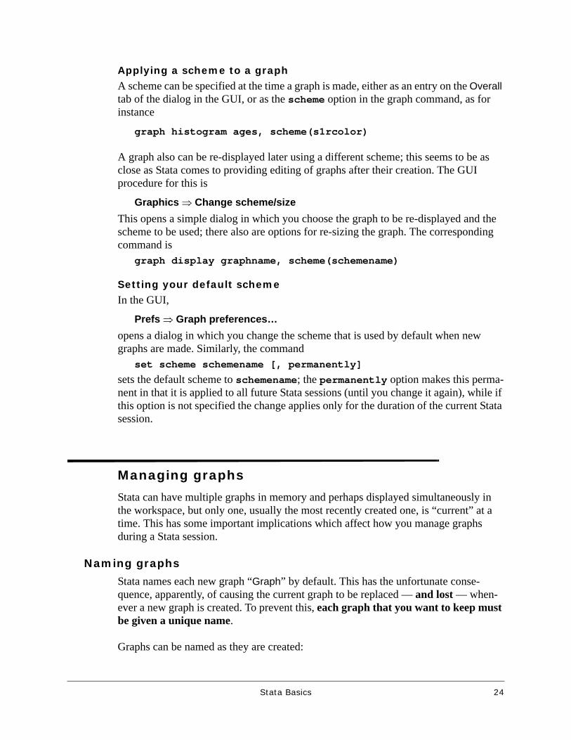
A more controlled and controllable way to arrange multiple graphs is by the combine or Table of graphs facility, which combines two or more existing graphs as panels of a new graph, with considerable user control over the layout of these panels. In the GUI, use

Graphics ⇒ Table of graphsThis opens the dialog window shown below:

The only required part of this dialog is the list of Graphs to combine. These can be typed in directly, or can be selected using the scroll-list of Include memory graph(s) and/or the Browse button of Include graph saved on disk; if graphs are selected in either of these latter two boxes, the selections need to be moved to the Graphs to combine entry by clicking the Add selected graph(s)… buttons above the Include … boxes. Other options on this Main tab, and on the other tabs, control the layout, labeling and appearance of the new multipanel graph.

Stata Basics 26

Stata graphing: general features: Saving, exporting, and printing graphs

The command to create such a table of graphs is

graph combine graph1 graph2 …

Saving, exporting, and printing graphs

Saving graphs

Graphs saved to disk in Stata’s own graph format can be reopened into Stata later, for instance for inclusion into a table of graphs. The filename extension for Stata graphs is .gph. In the GUI, use

File ⇒ Save graph…which opens a typical save-as dialog window. A graph saved this way, in the default Stata format, can later be opened in Stata using

File ⇒ Open graph…

The equivalent commands are

graph save “path_and_filename” , replace

andgraph use “path_and_filename”

Stata Basics 27

Stata graphing: general features: Saving, exporting, and printing graphs

Exporting graphs

Stata can export graphs in a variety of standard formats; in Windows these include: Windows metafile (wmf), enhanced metafile (emf), portable networks graphics (png), TIFF, PostScript, and EPS. In the GUI, simply choose the desired format in the Save as type: box of the Save graph dialog. This sort of export apparently cannot be done by commands.

It also works, with at least some other applications, including MS Word, to copy a Stata graph and paste it into an open document in the other application. To copy a graph, select it (i.e. make it the active window), right-click on it, the select Copy. Pasting into the other application will work better if you use “Special Paste” rather than the regular paste; pasting as an “enhanced metafile” may or may not work, depending on the application being pasted into, but if it doesn’t, try pasting as a regular metafile.

Printing graphs

A graph can be printed directly (as opposed to first exporting it as above) by either right-clicking on it and selecting Print, or by File ⇒ Print! ⇒ Graph(graphname). As with exporting graphs, it does not appear that printing can be done from the command line.

Stata Basics 28

EXPLORING AND DESCRIBING DISTRIBUTIONS

It does not appear that Stata has procedures to simultaneously produce graphs and descriptive statistics.

Plots of distributions

Histograms

GUI

Graphics ⇒ Easy graphs ⇒ HistogramGraphics ⇒ Histogram

The first route (Easy graphs) does not allow use of by variables, while the second does. Otherwise, for the purposes of the Biometry course, these two procedures are equivalent. Both allow density curves (normal distribution and/or nonparametric) to be added, though I don’t generally like to do this. The second route provides much more detailed control over appearance (e.g. of axes).

BinningThe most important aspect of a histogram to be able to modify is the “binning”: the number and location of the bars. In the Easy graphs version of a histogram, this is done on the Options tab of the dialog; in the full version gotten directly from the Graphics menu, binning controls are on the Main tab. In either case, the aspects that can be specified are the number of bins, their width, and the starting point, i.e. the lower limit of the first bin. You cannot explicitly control cutpoints or midpoints, but by choosing the lower limit and the bin widths you can accomplish the same thing.

Command[graph] histogram variable

BinningUse one or more of the following options:

bin(n) width(n) start(n)

where the ns are numeric values specifying the number of bins, width of bins, or lower limit of the first bin, respectively.

Comparing distributions

In the following I assume the data are in the “stacked” layout: all observations of the variable of interest in one column, with the groups defined by the values in one or

Stata Basics 29

more other columns. If the distribution to be compared are in separate columns (the “unstacked” layout), simply make separate histograms (i.e. separate graphs); force a uniform binning to facilitate comparison.

Separate panelsIn the GUI, the “Easy graphs” version of histograms does not accept by variables; use

Graphics ⇒ HistogramOn the By tab, list the grouping variable(s) in the Variables: box. If there are only two or three groups, comparison can be facilitated by having the histograms aligned one above the other; to request this, switch the Layout: setting (also on the By tab) to Columns.

The command for a histogram with a “by” variable is

histogram var , by(byvar [, cols(1)]

where var is the variable to be graphed, byvar is the grouping variable (there can be more than one), and , cols(1) is the option command to put the panels in a single column.

OverlaidTo overlay histograms (for the same variable in different groups), the menu selection is

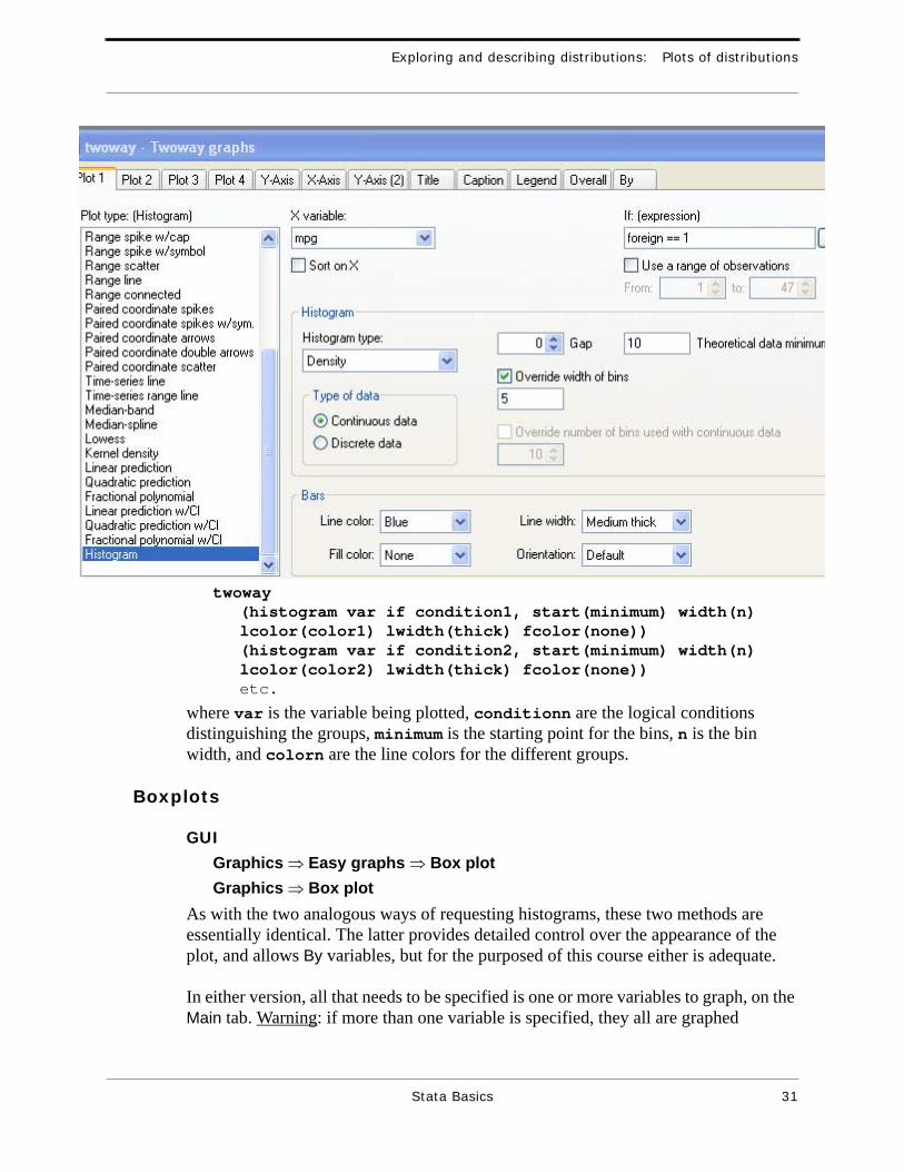
Graphics ⇒ Overlaid twoway graphs(never mind that histograms are somewhat out of place in a procedure for two-way graphs). The dialog window for this procedure (shown below) allows up to four plots to be superimposed; each plot is specified on a separate tab. For each plot, its type is selected from the list at the left; the rest of the items on the tab then change to those appropriate for the chosen plot type.

To compare histograms in a usable overlaid plot, several optional settings are needed in the tabs for each of plots:

• Use different If expressions to select different groups for the different plots.• Check the Override width of bins box, set a common bin width, and set a common

Theoretical data minimum; if these aspects are not set the same for all the plots, they will not align properly.

• Set the Fill color for the Bars to None; fills are opaque so any filled bar will hide any bars (of other of the overlaid plots) which are lower than it. You probably also will want to set thick Line width for the bars, and a different Line color for each of the plots.

Note that specifying a By variable (on the By tab) does not cause graphs for the differ-ent values of that variable to be overlaid; rather, they are put in separate panels.

Due to the number of options required for overlaid histograms to be usable, the com-mand is complicated:

Stata Basics 30

Exploring and describing distributions: Plots of distributions

twoway(histogram var if condition1, start(minimum) width(n) lcolor(color1) lwidth(thick) fcolor(none))(histogram var if condition2, start(minimum) width(n) lcolor(color2) lwidth(thick) fcolor(none))etc.

where var is the variable being plotted, conditionn are the logical conditions distinguishing the groups, minimum is the starting point for the bins, n is the bin width, and colorn are the line colors for the different groups.

Boxplots

GUI

Graphics ⇒ Easy graphs ⇒ Box plotGraphics ⇒ Box plot

As with the two analogous ways of requesting histograms, these two methods are essentially identical. The latter provides detailed control over the appearance of the plot, and allows By variables, but for the purposed of this course either is adequate.

In either version, all that needs to be specified is one or more variables to graph, on the Main tab. Warning: if more than one variable is specified, they all are graphed

Stata Basics 31

Exploring and describing distributions: Plots of distributions

together, on the same axis; unless their scales are similar this may create a useless graph.

Command[graph] box varlist

where varlist is the list of variables to graph.

Comparing distributions

Unstacked dataIf the groups are in separate columns (i.e. the data are unstacked), simply list the several columns as the variables to be graphed (in either the GUI dialog or the command).

Stacked dataIn the GUI (in either the Easy graphs or Graphics ⇒ Box plot version), go to the Over (or Over groups) tab and list the grouping variable(s) in the boxes for Over 1 and Over 2. (To use three grouping variables, use the Graphics ⇒ Box plot version, and toggle the ‘Over 1 and Over 2’ box to ‘Over 3 and Yvaroptions’.)

For the command, simply add an over(groupvars) option, e.g.

box mpg, over(foreign)

Normal quantile-quantile plots

There are two routes through the GUI menus to obtain a normal quantile plot:

Graphics ⇒ Distributional graphs!!!! ⇒ Normal quantile plotor

Statistics ⇒ Summaries, tables, & tests!!!! ⇒ Distributional plots & tests!!!! ⇒ Normal quantile plot

The dialog is very simple: just specify the variable to be graphed.

The corresponding command also is very simple:

qnorm varname

where varname is the variable to be graphed.

Note that this plot puts the observed values on the vertical (Y) axis and the normal-scores on the horizontal (X) axis (which Stata labels “Inverse Normal”); this is the opposite orientation to the NQQ plots made by Minitab.

Comparing distributions

The normal-quantile plot procedure does not accept By variables. Separate plots for different levels of a categorical variable (if the data are stacked) can be made by using If conditions to define the groups; if the groups are in separate columns (i.e. the data

Stata Basics 32

Exploring and describing distributions: Descriptive statistics

are unstacked), simply make separate plots. These plots will be in separate windows, but could be combined as panels in one graph using the Table of graphs procedure.

Charts for categorical variables

Graphics ⇒ Bar charts!!!! ⇒ Summary statisticsOn the Main tab, for Statistic, select ‘count nonmissing’ for any variable that does not have any missing values. Then on the Over groups tab, specify the categorical variable of interest as Over 1.

graph bar (count) varname , over(groupvar)

where varname is some variable with no missing values, and groupvar is the cate-gorical variable of interest.

Descriptive statistics

The most direct ways to get descriptive statistics in Stata do give much control over which descriptive statistics it reports, giving only two rather extreme choices, as follows.

A wider range of statistics, and more ability to pick and choose among them, is pro-vided by two of the methods described later for comparing distributions (tabstat and table).

Basic

To get a minimal set of statistics — sample size n, sample mean , sample standard deviation s, and sample minimum and maximum — use

Statistics ⇒ Summaries, tables, & tests!!!! ⇒ Summary statistics!!!! ⇒ Summary Statistics

and simply list the variables for which you want the statistics (or leave this blank to get statistics for all the quantitative variables in the data set).

The equivalent command (clearly much quicker to submit than the preceding trek through four menu selections before getting to the dialog) is

summarize [var1 [var2 …] ]

where varn are the variables for which statistics are desired; if none are listed, statis-tics are given for all quantitative variables in the data set.

Detailed

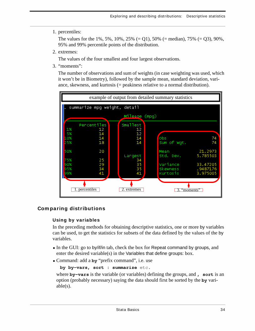
To get additional statistics, in the GUI click on radio-button on the summarize dialog that says Display additional statistics, or add the option , detail to the summarize command. This produces a very extensive set of statistics:

x

Stata Basics 33

Exploring and describing distributions: Descriptive statistics

1. percentiles:The values for the 1%, 5%, 10%, 25% (= Q1), 50% (= median), 75% (= Q3), 90%, 95% and 99% percentile points of the distribution.

2. extremes:The values of the four smallest and four largest observations.

3. “moments”:The number of observations and sum of weights (in case weighting was used, which it won’t be in Biometry), followed by the sample mean, standard deviation, vari-ance, skewness, and kurtosis (= peakiness relative to a normal distribution).

Comparing distributions

Using by variables

In the preceding methods for obtaining descriptive statistics, one or more by variables can be used, to get the statistics for subsets of the data defined by the values of the by variables.

• In the GUI: go to by/if/in tab, check the box for Repeat command by groups, and enter the desired variable(s) in the Variables that define groups: box.

• Command: add a by “prefix command”, i.e. useby by-vars, sort : summarize etc.

where by-vars is the variable (or variables) defining the groups, and , sort is an option (probably necessary) saying the data should first be sorted by the by vari-able(s).

example of output from detailed summary statistics

1. percentiles 2. extremes 3. “moments”

Stata Basics 34

Exploring and describing distributions: Descriptive statistics

Using tables

There are several ways to produce tables in which the rows (and optionally columns) represent the levels of one or more grouping variable(s), and the table-cell contents are descriptive statistics for one or more other, quantitative, variables. These methods differ in the sets of statistics that are available, as well as in the format of their output.

‘tabsum’This method has the simplest dialog but produces a very limited set of statistics: only the sample mean, standard deviation, and sample size, and only for one variable. The menu selections for this method are

Statistics ⇒ Summaries, tables, & tests!!!! ⇒ Tables!!!! ⇒ One/two-way table of summary statistics

In the resulting dialog the grouping variable(s) are specified as Variable 1: and (optionally) Variable 2:, and the variable for which the statistics are desired is named in the Summarize variable: box. There are check-boxes to eliminate one or more of the statistics, but no options for getting additional statistics.

The corresponding command is

tabulate groupvariable , summarize(variable)

‘tabstat’Note that a grouping variable is not required for this method, so it can also be used to get greater control over the statistics produced even when no grouping is desired.

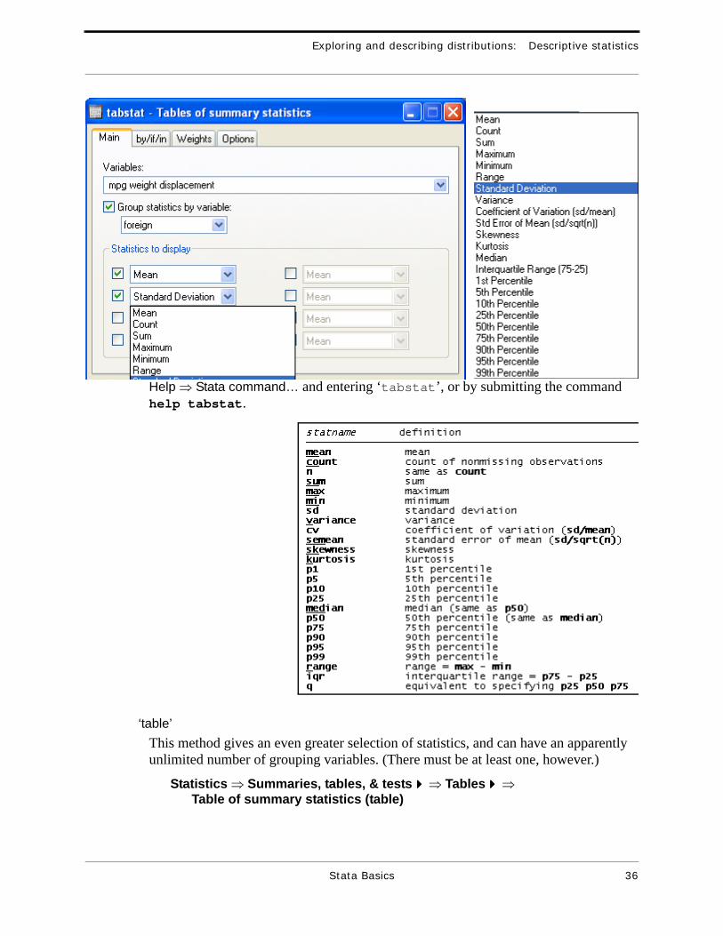
This method can produce a large selection of statistics, for more than one variable at a time, though with only one grouping variable. The menu selections are

Statistics ⇒ Summaries, tables, & tests!!!! ⇒ Tables!!!! ⇒ Table of summary statistics (tabstat)

In the dialog (see below) the quantitative variables for which statistics are desired are listed in the Variables: box. To get the statistics separately for the levels of another variable, the Group statistics by variable: box must be checked and the grouping vari-able listed below that.

In the Statistics to display part of the dialog, each of the check boxes has a correspond-ing box (with pop-up scroll list) in which the particular statistic is specified; as shown at the right of the example dialog below, the list of available statistics is extensive.

The command for this method is

tabstat var1 [var2 …], statistics(stat1 [stat2 …]) by(groupvar) columns(variables)

where varn is/are the quantitative variables for which the statistics are to be produced, statn is/are the desired statistics, and groupvar is the grouping variable. The keywords for the various statistics are listed below and can be gotten by

Stata Basics 35

Exploring and describing distributions: Descriptive statistics

Help ⇒ Stata command… and entering ‘tabstat’, or by submitting the command help tabstat.

‘table’This method gives an even greater selection of statistics, and can have an apparently unlimited number of grouping variables. (There must be at least one, however.)

Statistics ⇒ Summaries, tables, & tests!!!! ⇒ Tables!!!! ⇒ Table of summary statistics (table)

Stata Basics 36

Exploring and describing distributions: Descriptive statistics

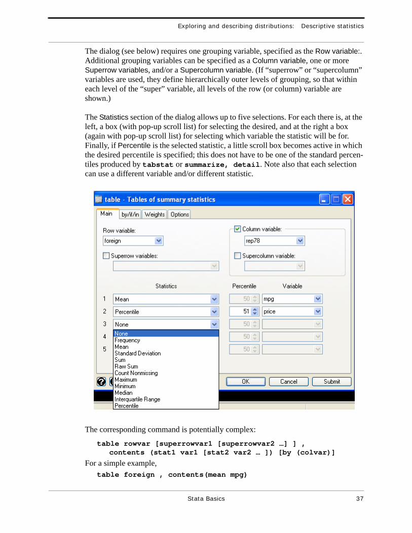
The dialog (see below) requires one grouping variable, specified as the Row variable:. Additional grouping variables can be specified as a Column variable, one or more Superrow variables, and/or a Supercolumn variable. (If “superrow” or “supercolumn” variables are used, they define hierarchically outer levels of grouping, so that within each level of the “super” variable, all levels of the row (or column) variable are shown.)

The Statistics section of the dialog allows up to five selections. For each there is, at the left, a box (with pop-up scroll list) for selecting the desired, and at the right a box (again with pop-up scroll list) for selecting which variable the statistic will be for. Finally, if Percentile is the selected statistic, a little scroll box becomes active in which the desired percentile is specified; this does not have to be one of the standard percen-tiles produced by tabstat or summarize, detail. Note also that each selection can use a different variable and/or different statistic.

The corresponding command is potentially complex:

table rowvar [superrowvar1 [superrowvar2 …] ] ,contents (stat1 var1 [stat2 var2 … ]) [by (colvar)]

For a simple example,table foreign , contents(mean mpg)

Stata Basics 37

Exploring and describing distributions: Descriptive statistics

will produce a simple table with only the mean mpg, for each category of the “foreign” variable. More complexly, the selections in the dialog window above would yield the command

table foreign, contents(mean mpg p51 price) by(rep78)

Note that the keyword for any percentile, in this command, is pn where n specifies the percentile.

Categorical variables

Several of the “table” procedures described above can be used to tabulate a categorical variable, i.e. to count how many observations there are for each of its levels. The simplest method (for a single categorical variable) is

Statistics ⇒ Summaries, tables, & tests!!!! ⇒ Tables!!!! ⇒ One-way tableswhich requires only that the variable of interest be specified. The corresponding command is

tabulate variable

Stata Basics 38

DESCRIBING RELATIONSHIPS

This chapter focuses on relationships between two quantitative variables. Describing the relationship between one quantitative variable and one or more categorical vari-ables amounts simply to comparing (between levels of the categorical variable) descriptions of the distribution of the quantitative variable, using methods presented in the “Comparing distributions” parts of the preceding chapter. Describing relationships between two categorical variables is covered at the end of this chapter.

Scatterplots

GUI: Graphics ⇒ Easy graphs!!!! ⇒ ScatterplotCommand: scatter Yvar Xvar

Only the Y and X variables need to be specified. Specifying more than one Y variable will produce overlaid plots of the Ys against the single X.

Smoothers

Stata provides at least three sorts of scatterplot smoothers:

• LowessThe usual Lowess smoother, as in Minitab or S-Plus.

• Median-bandThis is similar to what our textbook calls a “median trace”: the data are divided into segments along the X axis, and for each segment the median of the Ys is plotted against the median of the Xs.

• Median-splineThis is a “spline” smoothing of the median-band trace.

With the default settings the latter two appear to smooth the data less than does Lowess, but the degree of smoothing can be adjusted in all three.

Lowess

The Lowess smoother can be gotten either directly or using the “overlaid twoway plots” general procedure. For the direct method, the menu selections are

Graphics ⇒ Smoothing and densities!!!! ⇒ Lowess smoothingIn this dialog, simply specify the Dependent variable and Independent variable, and optionally Specify the bandwidth. The corresponding command is

lowess Yvar Xvar [, bwidth(n)]

Stata Basics 39

The alternative method is to overlay the smoother over a scatterplot. The menu selec-tions for this are

Graphics ⇒ Overlaid twoway graphs ⇒ Lowess smoothingThe specify the simple scatterplot as one of the numbered plots in this dialog, and for another of the numbered plots, select Lowess as the plot type, name the X variable and Y variable, and (optionally) change the Bandwidth. There corresponding command is:

twoway (scatter Yvar Xvar) (lowess Yvar Xvar [, bwidth(n)] )

The “bandwidth” of the Lowess smoother is essentially what fraction of the points go into the “weighted running average” calculated for each given point. The values is a decimal fraction, and the smaller it is the less the plot is smoothed.

Median-band and median-spline

The two median-based smoothers can only be gotten using the “overlaid twoway graphs” method described above for the Lowess smoother. In the GUI dialog simply select the desired plot-type (note that you could overlay a Lowess and another smoother or two), specify the X variable and Y variable, and (optionally) adjust the smoothing. For the “median-band” smoother, smoothness is controlled by the Number of bands, with more bands giving less smoothing. For the “median-spline” smoother there is both the Number of bands control and a Number of points between knots control; in my (admittedly limited

Distinguishing groups

It often is of interest to compare the relationship between two quantitative variables, among two or more groups of observations. (In effect, this examines the three-way relationship between the two quantitative variables and a categorical variable defining the groups.) Graphically, this is done by comparing the two scatterplots, typically overlaid and using different symbols for the different groups.

In the GUI, use

Graphics ⇒ Overlaid twoway graphsSpecify the two or more sets of data on different Plot n tabs of the dialog. If the data are in the “wide” (“unstacked”) layout, such that the observations for the different groups are in different pairs of columns, simply specify the appropriate columns for each plot. If the data are in the “narrow” (“stacked”) layout, so that the data for the different groups are different rows of the same pair of columns, use the If: (expression) parts of the dialogs to limit each plot to the desired observations.

There are two command-line methods for overlaying scatterplots for groups. One is:

twoway (scatter plot1specifications) (scatter plot2specifications) …

The alternative command uses the || operator:scatter plot1specifications || plot2specifications …

Stata Basics 40

Describing relationships: Correlation coefficient

In both commands plotnspecifications means the Y and X variables and any options for the nth plot. If the data are in the “long” (“stacked”) layout, these options will include if conditions to identify the observations for that plot. The … in the commands means that more than two groups can be overlaid by simply stringing on additional (scatter …) or || scatter … elements.

Smoothers (e.g. Lowess) can be overlaid on these “grouped” scatterplots simply by adding more plots of the desired smoother plot-type. Note that if the data are in the “long” (“stacked”) layout, a smoother based on all the data (i.e. ignoring the grouping) can be added by omitting the if specification.

Correlation coefficient

There are two ways to get correlation coefficients (matrices of pairwise correlations if more than two variables are specified. These methods differ somewhat in the optional statistics that can be produced but using their defaults just to get the coefficients as descriptive statistics gives essentially identical output. In the GUI the two methods are

Statistics ⇒ Summaries, tables, & tests!!!!⇒ Summary statistics!!!! ⇒ Pairwise correlations

andStatistics ⇒ Summaries, tables, & tests!!!!⇒ Summary statistics!!!! ⇒

Pairwise correlationsthen specify the two (or more) variables. The corresponding commands are

pwcorr varlist

andcorrelate varlist

where varlist is the list of variables to be correlated.

Regression

Statistics ⇒ Linear models and related!!!!⇒ Linear regressionthen specify the Dependent variable: and (single) Independent variables:.

Regression plot

A linear least-squares regression fit is a standard twoway graph plot type. The Over-laid twoway graphs dialog therefore can be used to combine the fitted regression with the scatterplot.

Stata Basics 41

Describing relationships: Regression

The command for the fitted-line plot is lfit; this can be used in either of the ways of invoking overlaid plots, i.e.

twoway (scatter Yvar Xvar) (lfit Yvar Xvar)

orscatter Yvar Xvar || lfit Yvar Xvar

Alternatively, the fitted values can be stored (see below) and plotted against the X variable, using the Line plot type; be sure to sort the data on the X variable first.

Residual plots

Residuals vs. fits or explanatory variable

A couple of scatterplots of residuals can be made quite easily. After performing a regression (as above), its residuals can be plotted against its fitted values using, in the GUI,

Statistics ⇒ Linear models and related!!!!⇒ Regression diagnostics!!!! ⇒ Residual-versus-fitted plot

orGraphics ⇒ Regression diagnostic plots!!!! ⇒ Residual-versus-fitted

Nothing needs to be specified; simply click OK.

The equivalent commands is ridiculously simple:

rvfplot

The residuals can be plotted against the independent variable using

Statistics ⇒ Linear models and related!!!!⇒ Regression diagnostics!!!! ⇒ Residual-versus-predictor plot

or Graphics ⇒ Regression diagnostic plots!!!! ⇒ Residual-versus-predicted

For this plot you need to select the independent variable (this is required because the same dialog can be used for multiple regression, in which there are multiple predictors that could be used).

The corresponding command again is very simple:

rvpplot Xvar

Note that both these commands use the residuals and fits from whatever regression was most recently conducted. (Its internal computational results are kept lurking in memory somewhere, though I don’t know how to access them directly.)

Stata Basics 42

Describing relationships: Regression

On the final menu selections to get to these two plots you will see various other residual plots; these are for more advanced diagnostic purposes, especially in multiple regression, and some of them will be covered in Advanced Biometry.

Other residual plots

As far as I can tell any other residual plots (e.g. distribution plots such as histograms or boxplots, or plots of residuals vs. any other variable) can only be made by saving the residuals (and fits, if needed) as described below, and then constructing the plot using those stored variables.

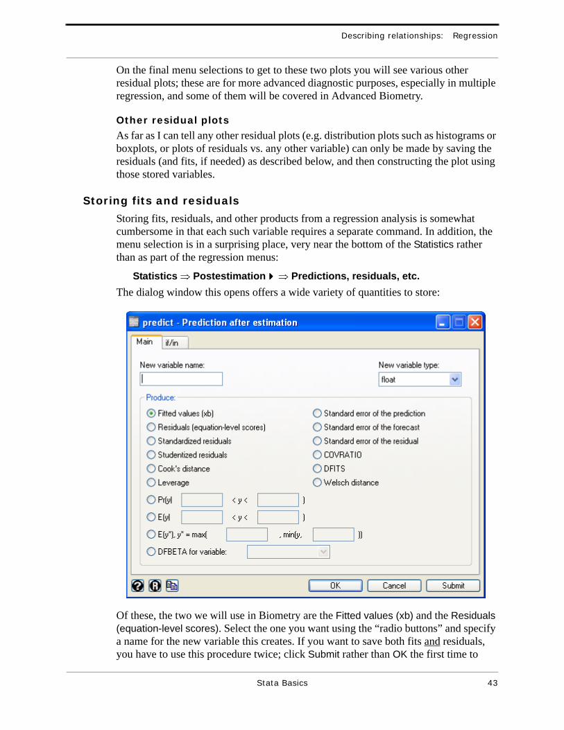
Storing fits and residuals

Storing fits, residuals, and other products from a regression analysis is somewhat cumbersome in that each such variable requires a separate command. In addition, the menu selection is in a surprising place, very near the bottom of the Statistics rather than as part of the regression menus:

Statistics ⇒ Postestimation!!!! ⇒ Predictions, residuals, etc.The dialog window this opens offers a wide variety of quantities to store:

Of these, the two we will use in Biometry are the Fitted values (xb) and the Residuals (equation-level scores). Select the one you want using the “radio buttons” and specify a name for the new variable this creates. If you want to save both fits and residuals, you have to use this procedure twice; click Submit rather than OK the first time to

Stata Basics 43

Describing relationships: Categorical variables

avoid having to re-open the dialog. (The parenthetical xb for fits is simply the standard matrix notation for computing the fits; the parenthetical equation-level scores for residuals just means these are the residuals as directly defined from the regression equation, i.e. Yi − (b0 + b1xi).)

The equivalent commands are

predict newvarname , xb

for the fits, andpredict newvarname , residuals

for the residuals.

Categorical variables

Data layouts

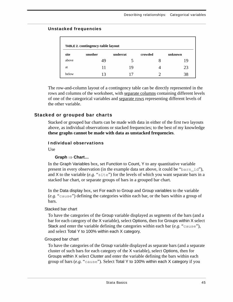
There are at least three ways data for a two-way contingency table, i.e. describing the relationship between two categorical variables, can appear in the worksheet. What can be done with the data, as well as how it is done, depends on the layout.

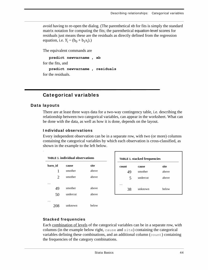
Individual observations

Every independent observation can be in a separate row, with two (or more) columns containing the categorical variables by which each observation is cross-classified, as shown in the example to the left below.

Stacked frequencies

Each combination of levels of the categorical variables can be in a separate row, with columns (in the example below right, cause and site) containing the categorical variables defining these combinations, and an additional column (count) containing the frequencies of the category combinations.

:

TABLE 1. stacked frequencies

count cause site

49 smother above

5 undercut above

…

38 unknown below

:

TABLE 1. individual observations

barn_id cause site

1 smother above

2 smother above

…

49 smother above

50 undercut above

…

208 unknown below

Stata Basics 44

Describing relationships: Categorical variables

Unstacked frequencies

The row-and-column layout of a contingency table can be directly represented in the rows and columns of the worksheet, with separate columns containing different levels of one of the categorical variables and separate rows representing different levels of the other variable.

Stacked or grouped bar charts

Stacked or grouped bar charts can be made with data in either of the first two layouts above, as individual observations or stacked frequencies; to the best of my knowledge these graphs cannot be made with data as unstacked frequencies.

Individual observations

Use

Graph ⇒ Chart…In the Graph Variables box, set Function to Count, Y to any quantitative variable present in every observation (in the example data set above, it could be “barn_id”), and X to the variable (e.g. “site”) for the levels of which you want separate bars in a stacked bar chart, or separate groups of bars in a grouped bar chart.

In the Data display box, set For each to Group and Group variables to the variable (e.g. “cause”) defining the categories within each bar, or the bars within a group of bars.

Stacked bar chartTo have the categories of the Group variable displayed as segments of the bars (and a bar for each category of the X variable), select Options, then for Groups within X select Stack and enter the variable defining the categories within each bar (e.g. “cause”), and select Total Y to 100% within each X category.

Grouped bar chartTo have the categories of the Group variable displayed as separate bars (and a separate cluster of such bars for each category of the X variable), select Options, then for Groups within X select Cluster and enter the variable defining the bars within each group of bars (e.g. “cause”). Select Total Y to 100% within each X category if you

TABLE 2. contingency-table layout

site smother undercut crowded unknown

above 49 5 8 19at 11 19 4 23below 13 17 2 38

Stata Basics 45

Describing relationships: Categorical variables

want the bars to represent percentages within each level of the X variable (the one defining the different groups of bars).

Stacked frequencies

The bar charts are made as just described for individual observations, but in the Graph Variables box, set Function to Sum, and Y to the variable containing the frequencies.

Stata Basics 46