Stat for Mgmt Solutions for Exercises

STATISTICS for MANAGEMENT

By DR T N Srivastava & Ms Shailaja Rego

Solutions to Exercises

Chapter 2 1. A) Nominal, discrete B) Ordinal, discrete C) Ratio, discrete D) Ratio, Discrete E) Ordinal , Discrete 2.a) Qualitative Nominal Discrete b) Qualitative Ordinal Discrete c) Quantitative Ratio Continuous d) Qualitative Ordinal Discrete e) Qualitative Nominal Discrete f) Quantitative Ratio Continuous g) Quantitative Ratio Continuous h) Quantitative Ratio Continuous i) Qualitative Nominal Discrete j) Quantitative Ratio Continuous k)Quantitative Interval Continuous Chapter 4 1. 109.1143, 109.1143 2. Sales of all pain killers in 2005 = 80.4 Sales of all pain killers in 2006 = 111.2 Thus, Average growth for all = {( 111.2 – 80.4) / 80.4}× 100 = 38.3% 3. Minimum – 602.00 , First Quartile – 714.00, The Median – 993, Third Quartile – 1259.5 Maximum – 2451 4. Using the template on page 4.59, one obtains the basic statistics of the data as follows:

Basic Statistics Sum 683,795.00 Count 10.00 Max 79,021.00 Min 42,288.00 Arithmetic Mean 68,379.50 Median 76,075.00 Mode Geometric mean 66,933.09 Quartile 1 63,878.50 Quartile 2 76,075.00 Quartile 3 77,244.50 Percentile 69,998.02

Range 36,733.00 IQR 13,366.00 Population Variance 166,040,004.05 Sample Variance 184,488,893.39 Population Std Dev 12,885.65 Sample Std Dev 13,582.67 Coefficient of Variation 20%

The appropriate measures of variation are as follows: Arithmetic Mean = 68,379, Median = 76,075.00, IQR - 13,366.00, Sample Std Dev - 13,582.67, Coefficient of Variation (Sample s.d. / arithmetic mean) = (13,582.67/ 68,379.50) 19.86 or 20% 5. The compound annual growth rates are obtained by the Formula 4.7 G = 100 (Pn / P1 )

1/(n-1) = × 100 × {( Price in 2005 – Price in 1981) / ( Price in 1981)} ( 1/ 24

) Thus, CAGR for rice is obtained by formula 4.8 as = antilog { log 100 + ( 1/ 24 ) ( log 11.5 – log 4.5 ) } = 3.99 % Similarly for other items CAGRs can be obtained as Wheat = 5.42%, Sugar = 5.40% , Milk = 4.83% One can also Formula (4.5) on a scientific calculator to get the result. 6. i) Average life expectancy for all the countries = ( Total of lives of the populations of all the countries) / ( Total Population of all the countries) The numerator is found by multiplying life expectancy of each country by its population, and adding this product for all countries, and is equal to 211705.2. The denominator is equal to 3087.2 Thus, average life expectancy for all the countries = (211705.2) / 3087.2 = 68.58 ii) Average % of school enrolment for all the countries = {( Total school enrolments in all the countries) / ( Total Population of all the countries)} } × 100 The numerator is found by multiplying % of school enrolment of

each country by its population and dividing it by 100, and adding this product for all countries, and is equal to = . Thus, % of school enrolment for all the countries = = 67.4 iii) Average GDP per capita = Total GDP of all countries / Total Population of all countries The numerator is found by multiplying Per capita GDP of each country by its population and, and adding this product for all countries, and is equal to = Total Population = Thus, average GDP per capita = = 13757 iv) Average percentage of urban population = {Total urban population / Total population}× 100 The numerator is found by multiplying % of urban population of each country by its population and dividing it by 100, and adding this product for all countries, and is equal to = . The denominator is equal to 308.72 7. For Jyoti : Mean = 80% CV = 9.05% For Anuj : Mean = 79% CV = 3.10% Their average is about the same but Anuj is more consistent in his performance than Jyoti. 8. Using Formula (4.6), we get the desired GM as

= Antilog {(1/6) {log 207 + log 198 + log 156 + log 140 + log 107 + log 196} = 163.0252 One can also Formula (4.5) on a scientific calculator. 9. Here, we use the Formula ( 4.7) to get average growth rate as

100 × ( 2 ) 1 / 4 = 100 × Antilog ( 1/ 4 ) log 2 = 18.92% 10. Average price = Total amount paid for all the units / Number of units purchases = 60,000 / ( 10000/10 + 10000/11 + 10000 / 12 + 10000/ 15 + + 10000/18 + 10000 / 20) = 60000 / 4464.65 = Rs. 13.44 11. By using the template on page 4.59, the basic statistics for the two sets of data “Before” and “After” , the following results are obtained

Before Arithmetic Mean 52.64

Variance 133.89

Standard Deviation 11.10

Coefficient of Variation 21%

After Arithmetic Mean 51.50

Variance 134.00

Standard Deviation 11.58

Coefficient of Variation 22%

Mean has reduced by 1.14 days, s.d. is slightly increased by 0.48 . CV. i.e. relative variability is increased by 1%. 12. By using the template on page 4.60, or using the formulas 4.2, 4.12, 4.13, and 4.22, we get the following results:

Basic Statistics Sum(FX) 615.00 Count (Sum F) 60.00 Arithmetic Mean 10.25 Median 9.00

Variance 33.69 Standard Deviation 5.80 Coefficient of Variation 57%

Rating is 66 ROI 10%.33% Mean - 10.25 , Median - 9.00, Coefficient of variation - 57% ROI 12% Rating : 66.33% 13. Weighted Average Rate of Interest or Cost of Funds = = ( Total Interest Earned ) / ( Total Outstanding Deposits) Rate (%) Amount Outstanding (in Crores of Rs.) 0 27 . 3.5 39 - - months 5.0 61 6 months – 1 year 6.0 46 1 year – 3 years 7.0 32 3 years – 5 years 8.0 10 Over 5 years 9.5 32 The numerator is found by summing the product ( Rate of Interest × Deposits Outstanding) for each range of interest. The details of type or maturity period of deposits are not required in the calculation. Thus, the required answer is 5.366% . 14. Company A

Length of Life(in hrs.)

Middle Point of Life Interval (xi

)

Company Company B(fi

A(f i ) )

1500 – 2000 1750 16 18 2000 – 2500 2250 26 22 2500 – 3000 2750 8 8

Total 50 48

Basic Statistics Sum(FX) 108,500.00 Count (Sum F) 50.00 Arithmetic Mean 2,170.00 Median 2,173.08 Variance 113,600.00 Standard Deviation 337.05 Coefficient of Variation 16%

Company B

Basic Statistics Sum(FX) 103,000.00 Count (Sum F) 48.00 Arithmetic Mean 2,145.83 Median 2,136.36 Variance 124,565.97 Standard Deviation 352.94 Coefficient of Variation 16%

(i) Bulbs of Company A (mean 2170) have more life than those of Company B (ii) Both Companies are same for uniformity (CV 16%) 15. Average increase per worker per annum is 21130/- Impact on Coefficient of Variation 16. Average Monthly Income Per Family = ( Total Income of all Families) / Number of Families

= 3,737,500.00 / 200 = Rs.18,687.50

Basic Statistics Sum(FX) 3,737,500.00 Count (Sum F) 200.00 Arithmetic Mean 18,687.50 Median 20,000.00 Variance 92,496,093.75 Standard Deviation 9,617.49 Coefficient of Variation 51%

New


Per family 18575, per Earning Member 12383.33 Per capita 6191.667 Per Earning member = Total Income of All Persons or Families) / ( Total Number of Earning Members) = 6,735,000.00 / 300

Basic Statistics Sum(FX) 6,735,000.00 Count (Sum F) 300.00 Arithmetic Mean 22,450.00 Median 20,000.00 Variance 124,122,500.00 Standard Deviation 11,141.03 Coefficient of Variance 50%

Per Capita = ( Total Income of All Persons or Families) / ( Total Number of Persons) =


New i) Per family =18,687.50 ii) Per Earning members = 22,450.00 iii) Per Capita = 21,933.33 17. For calculation of median rate of return, the Table is reconstructed as follows :

Rate of Interest

March Cumulative Amount

2001 Cumulative % to Total

March Cumulative Amount

2006 Cumulative % to Total

Less than 8%

261 4 376 2.2

8 – 9 383 2 536 3.11 9 – 10 1263 13 2682 15.7 10 – 11 1263+906= 14 4132 24.1 11 – 12 1700 26 1236 7.2 12 – 13 1466 22 814 4.8 13– 14 716 11 997 5.8 14 – 15 406 6 1669 9.7 More

than 15 123 2 4697 27.4

The median can be calculated both with the help of columns of “ Cumulative

amount” or “ Cumulative % to Total” Median Rate of Return on Funds i) 11.66 (2001) ii ) 11.68 (2006) 18. Yes, variation can be measured by “ Coefficient of Variation” , and can be calculated either with the help of Formula ( 4.22 ) or template = 49% . Chapter 5 1 ( a ) The requisite probability = ( Number of Females opposed to the proposal) / Total number of employees = 1200 / 5000 = 0.24 ( b ) The requisite probability = ( Number of Employees neutral to the proposal) / Total number of employees = 600 / 5000 = 0.12 (c ) The requisite probability = ( Number of Females opposed to the proposal) / Total number of female employees = 1200 / 2000 = 0.60 ( d ) The requisite probability = ( Number of Employees opposed to the proposal) / Total number of employees = 2000 / 5000 = 0.40 2. Given P(Neither TV nor Fridge) = 175/500 = 0.35, Therefore, P(Either TV or Fridge or Both) = 1 – 0.35 = 0.65 By Theorem of Total probability P ( TV or Fridge or Both) = P(TV) + P(Fridge) – P ( Both TV and Fridge) Thus, P( Both TV and Fridge) = 0.5 + 0.4 – 0.65 = 0.25

3. Given

P( Approach is Successful) = P(A) = 0.6

P( Expenditure within Budget) = P(B) = 0.5 P( Approach is successful and Expenditure is within Budget) = P (AB) = 0.30

Therefore, P( Either Approach Successful or expenditure within budget) = P(A + B)

= P ( A) + P(B) – P(AB) = 0.6 + 0.5 = 0.3

= 0.8

4. Here, the outcome i.e. IQ more than 110, is known and we have to find whether it is

that of a graduate or undergraduate. Thus, this exercise can be solved with the help of Bayes’ theorem. We use the following notation: A : IQ is more than 110 B1 : Student is a graduate B2 : Student is undergraduate

Given,

P (B1 ) = 0.4

P (B1 ) = 0.6

P ( A / B1 ) = 0.75

P ( A / B2 ) = 0.3

we have to find P(B1 / A) = ?

Therefore, using Bayes’ Theorem

P(B1 / A) )/()(

)/()1( 1

ii BAPBP

BAPBP

∑=

0.4 × 0.75

we get P(B1 / A) = -------------

0.4 × 0.75 + 0.6 × 0.3

= 0.625 5. The problem will be solved if any one or at least one solves the problem. We use the formula 5.6 on page 5.20 as follows: P ( At least One ) = 1 – P (none) Thus, the required probability = 1 – P ( none solves the problem) = 1 – P( A does not solve) × P( B does not solve) × P( C does not solve) (assuming independence of their attempts to solve and using Multiplication Theorem of Probability given by ( 5. 5) on page 5.19) = 1 – (1/2) × ( 2/3) ×(4/5) = 1 – 4/15 = 0.7333

6. The student is choosing the options randomly with equal chance 1/3 for each of the

three options.

(i) The student can solve 3 questions out of 5 questions in following ways:

1, 2 and 3; 1,2 and 4; 1,2 and 5; 2,3 and 4; 2,3 and 5; 3,4 and 5. 1, 3 and 4; 1,3 and 5; 1, 4 and 5; 2, 4 and 5 Assuming independence of solving or not solving each question, the probability of solving three questions and not solving two questions , by Multiplication Theorem of Probability (5.5) is (1/3) × (1/3) × (1/3) × (2/3) × (2/3) = 4 / 243 Since, all the ten ways of solving 3 out of 5 questions are mutually exclusive, we use Addition Theorem of Probability ( 5.2), and derive the required probability as ( 4 / 243 ) + (4 / 243) + (4 / 243) + (4 / 243) + (4 / 243) + (4 / 243) + (4 / 243) + (4 / 243) + (4 / 243) + (4 / 243) = 40 / 243 = 0.1646

(ii) The probability that all 5 questions are wrong is obtained by using Multiplication

Theorem of Probability as

( 2 / 3 ) × ( 2 / 3 ) × ( 2 / 3 ) × ( 2 / 3 ) × ( 2 / 3 )

= 32 / 243 = 0.1317 ( iii ) At least 4 correct questions can be solved in following five ways : ( a) Four correct questions and one wrong question 1, 2, 3, and 4( 5 wrong); 1, 2, 4 and 5(3 wrong); 1, 3, 4 and 5(4 wrong); 2, 3, 4, and 5( 1 wrong); The probability for each of these five ways is (1 / 81) × ( 2/ 3)

Thus, the probability of four correct questions is 10 / 243

( b ) Five correct questions: 1, 2, 3, 4, and 5

The probility for this is 1 / 243

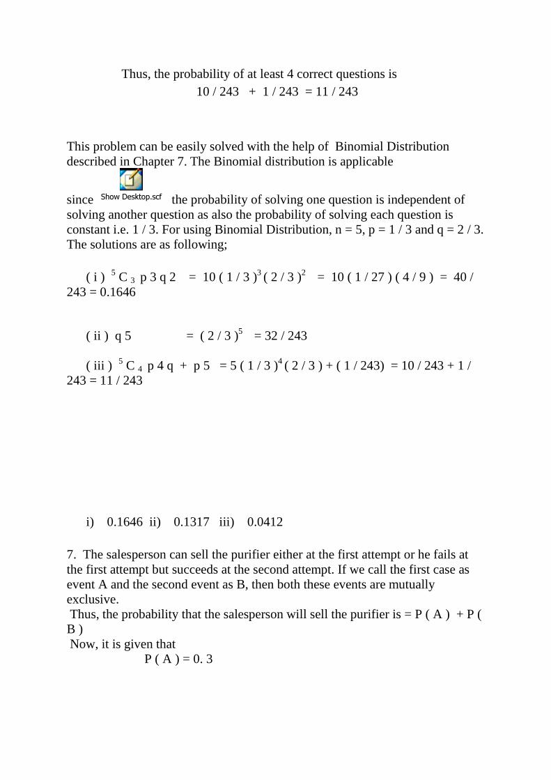
Thus, the probability of at least 4 correct questions is 10 / 243 + 1 / 243 = 11 / 243

This problem can be easily solved with the help of Binomial Distribution described in Chapter 7. The Binomial distribution is applicable

since Show Desktop.scf the probability of solving one question is independent of solving another question as also the probability of solving each question is constant i.e. 1 / 3. For using Binomial Distribution, n = 5, p = 1 / 3 and q = 2 / 3. The solutions are as following; ( i ) 5 C 3 p 3 q 2 = 10 ( 1 / 3 )3 ( 2 / 3 )2 = 10 ( 1 / 27 ) ( 4 / 9 ) = 40 / 243 = 0.1646

( ii ) q 5 = ( 2 / 3 )5 = 32 / 243 ( iii ) 5 C 4 p 4 q + p 5 = 5 ( 1 / 3 )4 ( 2 / 3 ) + ( 1 / 243) = 10 / 243 + 1 / 243 = 11 / 243

i) 0.1646 ii) 0.1317 iii) 0.0412 7. The salesperson can sell the purifier either at the first attempt or he fails at the first attempt but succeeds at the second attempt. If we call the first case as event A and the second event as B, then both these events are mutually exclusive. Thus, the probability that the salesperson will sell the purifier is = P ( A ) + P ( B ) Now, it is given that P ( A ) = 0. 3

P ( B ) = P ( does not sell at first attempt ) × P ( sells at second attempt) = (1.0 – 0.3) × 0.6 ( given) = = 0.7 × 0.6 = 0.42 Thus, the probability of selling the purifier = 0.3 + 0.42 = 0.72 8. This problem relates to Bayes’ Theorem as the event (making payment) is known to have , and we want to know the cause for this as to whether it was due to personally meeting or calling or writing. In Bayes’ Theorem notation A : Payment is received B1 : Meeting B2 : Calling B3 : Writing It is given that P(B1 ) = 0.6 P( B2 ) = 0.3 P( B3 ) = 0.1 P(A/B1 ) = 0.64 P(A/ B2 ) = 0.28 P(A / B3 ) = 0.08 Using Bayeys’ Formula ( 5 .7 ), we get

P(B1 / A) = )(

)( 1

AP

ABP = ∑ ×

×)/()(

)/()( 11

ii BAPBP

BAPBP = 75.048.0 = 0.64

P(B2 / A) = )(

)( 2

AP

ABP = ∑ ×

×)/()(

)/()( 22

ii BAPBP

BAPBP = 75.021.0 = 0.28

P(B3 / A) = )(

)( 3

AP

ABP = ∑ ×

×)/()(

)/()( 33

ii BAPBP

BAPBP = 75.006.0 = 0.08

P(pay) =0.75, P(personally/pay)= 0.64, P(call/pay)= 0.28, P(write/pay) = 0.08, 9. This problem relates to Bayes’ Theorem as the event (Diagnosed with Hematuria) is known , and we want to know the cause for this as to whether it was due to the

person suffering from kidney cancer or not suffering from kidney cancer A : Person diagnosed with Hematuria B1 : Person suffering from kidney cancer B2 : Person not suffering from kidney cancer It is given that P(B1 ) = 0.000002 P( B2 ) = 0.999998 P(A/B1 ) = 1.0 P(A/ B2 ) = 0.1 Using Bayeys’ Formula ( 5 .7 ), we get

P(B1 / A) = )(

)( 1

AP

ABP = ∑ ×

×)/()(

)/()( 11

ii BAPBP

BAPBP = 0.00002

10. This problem relates to Bayes’ Theorem as the event (the processed form having an error) is known to have happened. We want to know the cause for this i.e. whether it was caused by Clerk1 or Clerk2 or Clerk3 who processed all the forms. In Bayes’ Theorem notation A : The processed form has an error B1 : The form was processed by Clerk1 B2 : The form was processed by Clerk2 B3 : The form was processed by Clerk3 It is given that P(B1 ) = 0.4 P( B2 ) = 0.35 P( B3 ) = 0.25 P(A/B1 ) = 0.04 P(A/ B2 ) = 0.06 P(A / B3 ) = 0.03 Using Bayeys’ Formula ( 5 .7 ), we get P(B1 / A) = --------------- P(B2 / A) = --------------- P(B3 / A) = --------------- P(error) = 0.0445 P(Clerk 1 /Error) = 0.35955, P(Clerk 2 /Error) = 0.47191, P(Clerk 3 /Error) = 0.16854

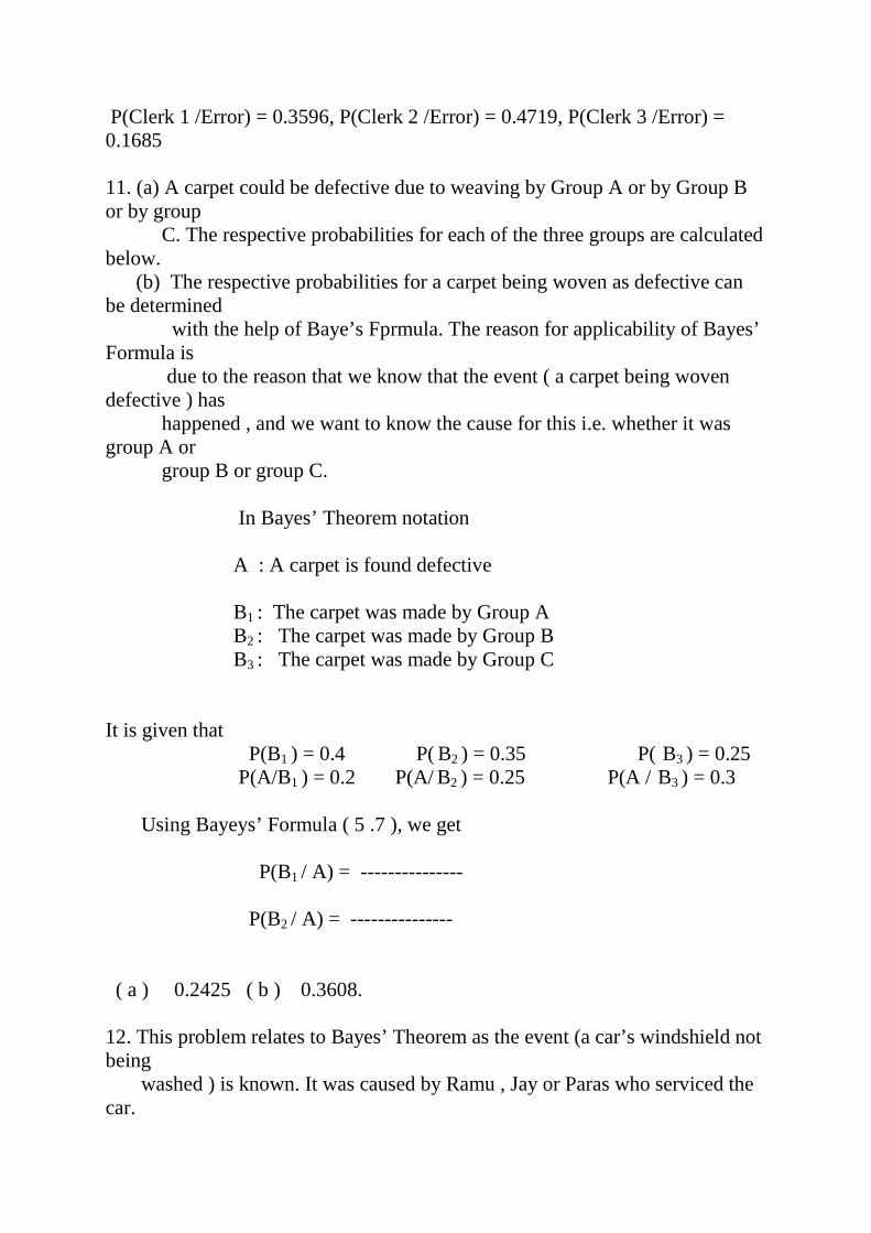
P(Clerk 1 /Error) = 0.3596, P(Clerk 2 /Error) = 0.4719, P(Clerk 3 /Error) = 0.1685 11. (a) A carpet could be defective due to weaving by Group A or by Group B or by group C. The respective probabilities for each of the three groups are calculated below. (b) The respective probabilities for a carpet being woven as defective can be determined with the help of Baye’s Fprmula. The reason for applicability of Bayes’ Formula is due to the reason that we know that the event ( a carpet being woven defective ) has happened , and we want to know the cause for this i.e. whether it was group A or group B or group C. In Bayes’ Theorem notation A : A carpet is found defective B1 : The carpet was made by Group A B2 : The carpet was made by Group B B3 : The carpet was made by Group C It is given that P(B1 ) = 0.4 P( B2 ) = 0.35 P( B3 ) = 0.25 P(A/B1 ) = 0.2 P(A/ B2 ) = 0.25 P(A / B3 ) = 0.3 Using Bayeys’ Formula ( 5 .7 ), we get P(B1 / A) = --------------- P(B2 / A) = --------------- ( a ) 0.2425 ( b ) 0.3608. 12. This problem relates to Bayes’ Theorem as the event (a car’s windshield not being washed ) is known. It was caused by Ramu , Jay or Paras who serviced the car.

We want to know the cause for this as to whether the car was serviced by Jay, Ramu or Paras as one of them would have washed the car. . In Bayes’ Theorem notation A : A car’s windshield is not washed B1 : The car was serviced by Ramu B2 : The car was serviced by Jay B3 : The car was serviced by Paras It is given that P(B1 ) = 0.3 P( B2 ) = 0.3 P( B3 ) = 0.4 P(A/B1 ) = 0.5 P(A/ B2 ) = 0.025 P(A / B3 ) = 0.05 Using Bayeys’ Formula ( 5 .7 ), we get P(B1 / A) = --------------- P(B2 / A) = --------------- P(B3 / A) = --------------- P(error) = 0.0445 P(Clerk 1 /Error) = 0.35955, P(Clerk 2 /Error) = 0.47191, P(Clerk 3 /Error) = 0.16854 P(Clerk 1 /Error) = 0.3596, P(Clerk 2 /Error) = 0.4719, P(Clerk 3 /Error) = 0.1685 i) P(Jay) = 0.1724 ii) P(Ramu) = 0.1379 P(Paras) = 0.2299 , P(Ramu or Paras) =0.3678 13. It is given that P ( Getting admission in A ) = 0. 4 = P(A), say P( Getting admission in B) = 0. 6 = P(B), say P ( Getting admission in both A and B) = 0.2 = P(AB) ( a ) He will be successful in getting admission if he gets admission in A or B or both A and B. Therefore, P ( Getting admission) = P(A) + P(B) – P (AB) = 0.4 + 0.6 – 0.2

= 0.8 (b) He will get admission only in one if he gets admission in one but does not get admission in the other. Thus, P ( Getting admission in only one Institute) = P ( Gets admission in A but does not get admission in B) + P (Gets admission in Bbut does not get admission in A) = P ( A ) ( 1 – P (B)) + P ( B) ( 1 – P (A) = 0.4 × 0.4 + 0.6 × 0.6 = 0.16 + 0.36 = 0.52 (c) P ( B / A) ( d) P ( A’ / B’ ) ( a) 0.8 (b) 0.6 ( c ) 0.5 ( d ) 0.5 14. This problem relates to Bayes’ Theorem as the event (An officer having passed the test) is known, ad we want to know the cause for this as to whether the officer had excellent or average confidential report. A : Person diagnosed with Hematuria B1 : Person suffering from kidney cancer B2 : Person not suffering from kidney cancer It is given that P(B1 ) = 0.000002 P( B2 ) = 0.9999998 P(A/B1 ) = 1.0 P(A/ B2 ) = 0.1 Using Bayeys’ Formula ( 5 .7 ), we get P(B1 / A) = --------------- P(B2 / A) = ---------------

a) 4/5 b)1/5 c) 1/3 d) Dependent 15. 0.75 16. 1.7 17. 1.59 18. 0.8 Chapter 7 1. 0.9185 2 (a ) 0.2048 ( b) 0.9933 ( c) 0.9421 3. 0.3456 4. (i) 0.0003 (ii) 0.3277 (iii) 0.6723 5. 0.0183 , 0.0001 6. ( i ) 0.0003 ( ii ) 0.0512 7. (i) 0.1353 (ii) 0.0166

8. 0.1404 9. 0.0778 10. (i) 0.1587 (ii) 0.13% (iii) 3.35 years 11 (i) 57.63% (ii) 7325.51 to 8674.4898 12. 126.92 13. (i) 0.8413 (ii) 2664.5

14. ( a ) 6.68% ( b ) 11289.71 15. 6 16. (i) 6.68% (ii) 15600/- 17 (i) 0.8571 (ii) 0.1429 (iii)0.1353 18 March 2001 Median of % to total = 11.35 March 2006 Median of % to total = 11.32

Count (Sum F) 100.00 Arithmetic Mean 17.50 Standard Deviation 9.94

Probability

Expected Frequency

<-5 0.0118 1.18 -5 – 5 0.0925 9.25 5 – 15 0.2964 29.64 15 – 20 0.3740 37.4

25 – 30 0.1861 18.61 >35 0.0392 3.92 �2 = 14.18 (ii)

x1 P(x1<X<x2)

Expected frequency

< 0 0.0165 1.650 – 5 0.0594 5.945 – 10 0.1555 15.5510 – 15 0.2547 25.4715 – 20 0.2607 26.0720 – 25 0.1669 16.6925 – 30 0.0668 6.68

>30 0.0196 1.96

��2 = 9.99

19. a) 0.7373 b) 0.0003 c) 4

20. 0.4557

Chapter 8 The exercises can be easily solved with the help of the template on correlation and regression analysis, given on CD. All that is required is to input the data as indicated in the template, and the result will come automatically on the screen. 1.

(i) Net profit = 983.4 + 0.055 × Net Sales r = 0.3663, r2 = 0.1342 (ii) Net Sales = 7818.07 + 3.02 ×P/E Ratio r = 0.0231, r2 = 0.0005. In both of the above cases, coefficients of determination are too low, and hence the regression equations may not be of much use to forecast Net Profit.

2. (i) 0.8909 (ii)0.7576 (iii) 0.8667 3. (a) (i) 0.104378 (ii) 0.146146 (iii) 0.073593

(b) (i) Beta of ICICI stock = 1.0273 This implies that the ICICI Stock is 2.73% more aggressive than BSE (ii)Beta of Reliance Industries stock = 0.8523 This implies that the Reliance Industries Stock gives 14.77 % less returns than BSE (iii)Beta of L & T stock = 0.981 This implies that the L & T Stock gives 1.866 % less returns than BSE 4. r = 0.8976, r2 = 0.8056 Thus there is a strong relationship. 80.56% of variation in Ice-cream is explained by variation in temperature.

5. r = 0.96265 r2 = 0.9267 Thus there is a strong relationship. 92.67% of variation in Amount of Insurance is explained by variation in Monthly Income. 6. Sales = 60.94737 + 4.302632 × Advertising Expenses Sales = 190.0263 for Advertising expenses 30 7. EPS = – 1.09622 + 0.0122 × Sales EPS = 0.2477 + 0.1415 × Advertising Expenses

8. r = 0.685315 It is desirable that the correlation is very high between the two rankings. Since it is only 0.685, they may not be able to recruit the right candidates 9 . (a) Sales = 6.5625 + 121.875 × Advertising Expenses (b) 128.4375 (c)0.97745 (d) 95.54% 10. 0.818182 Only 67% of variation in deposits is explained by customer satisfaction. The bank might be getting deposits due to other reasons also such as higher rate of deposits, confidence reposed by customers, flexibility in deposit schemes etc. 11. i) Demand = 188.522 – 7.33 × Price ii) 78.56 iii) 90.86% 12. a) Marks = 1 + 0.654 x I.Q. b) 79.515 c) 81.25% 13. Sales Revenue = 70.01 + 3.837 × Advertising Expenses, 98.715% 14. r = 0.6232 r2 = 0.3884 Chapter 9. 1. (a) Revenue = 2.83 × (Television Advertising ) + 90.1 (a) Revenue = 2.23 × (Television Advertising ) + 0.02 ×( Newspaper

Advertising ) + 91.7 (c) 100.65 Crores 2. Market Capitalisation = 0.31× Sales + 17.00 × Profit – 618407 . 3. No credit cards = No of credit cards = 0.63224× Family Size + 0.2158 × Family Income + 0.48169 SSE with Family Income= 3.049 (r2 = 0.8614 Adjusted r2 = 0.8059) SSE without Family Income = 5.486 (r2 = 0.7506) 4. Salary = 0.2378 × Age + 1.6839 × Sex + 4.19217 (With Sex as Dummy Variable) Error Ss = 203.819 r2 = 0.2355

Salary = 0.28475 × Age + 3.0+59 × Sex + 0.618 × IQ – 71.943 Error Ss = 181.223 r2 = 0.3202 Hence it has improved the regression model 5. Credibility Score = – 0 .1655 × Current Ratio + 0.0093 × Debt/ Asset Ratio – 0.1081 × Did Firm go bankrupt, earlier + 0.51414 6. Operating Profit = 0.21218 × Interest Income + 1.0548 × Non-Interest Income – 0.4348 r2 = 0.5183 SS Error = 5.90067 Operating Profit = 1.0675 × Interest Income + 1.20958 r2 = 0.0566 SS Error = 11.5558 Operating Profit = 1.0675 × Non Interest Income + 1.03378 r2 = 0.4736 SS Error = 6.4483 7. (a)

Company

EPS ( Rs.)

Sales

(Rs. in Crores)

Advertising Expenses

(AE) ( Rs. in Crores)

Operating Expenses

(OE) ( RS. in Crores)

1 1.00 100 80 35 2 2.00 175 120 28 3 1.50 89 72 30 4 3.00 225 175 20 5 3.25 300 240 25 6 3.5 320 230 35

(a) Fit the following regression equation: EPS = b0 + b1(Sales) + b2 (AE) + b3 (OE) (b) Formulate a suitable regression model with optimum number of variables to explain EPS.

8. The following Table gives some financial parameters and their growth of some Indian banks for the year 2005 as per Business Today’s Special issue of 26th February 2006.

Bank Net

Profit (Rs. Crores)

Net Profit

Average Working Funds (Rs. Crores)

Average Working Funds

Growth in Business

Growth in Business

Amount Rank Amount Rank Percentage

Rank

State Bank of India

4,304 1 433,849 1 20 25

ICICI Bank

2,005 2 131,075 2 47 2

Punjab National bank

1,410 3 106,302 3 20 24

Canara Bank

1,110 4 99,584 4 17 33

Oriental Bank of Commerce

761 5 46,066 12 32 6

HDFC Bank

666 8 44,335 13 30 7

Standard Chartered

602 10 34,801 16 18 28

Citibank 600 11 30,129 20 12 48 Corporation Bank

402 16 30,444 18 23 19

ABN AMRO

195 31 13,003 38 38 3

Estimate the relationship giving dependence of net profit on average working funds and growth in business. Test the significance of the regression coefficients as also of the relationship as a whole. Chapter 10 1. Since we want to test that the increase i.e. 5% of 6.5 = 0.325 in m1 is significant i.e. m2 > m1 + 0.325, we set up the alternative as follows:

H0 : m1 – m2 = 0.325 H1 : m1 – m2 < - 0.325 1x = 6.5 lakhs, s1 = 0.5, n1 = 20 2x = 7.0 lakhs, s2 = 0.75 , n2 = 25 Test Statistic as per calculations given on page 10. 56 = – 0.8954 Ans : Do not reject i.e. there is no significant increase in the salaries 2. This exercise relates to finding confidence interval for population proportion. As per fFormula 10.4, the confidence limits at α % are iven on page , the requisite formula is

n

qpzp 2/α+ where ( 1 – α )% is the level of confidence.

Here, n = 500, p = 0.3 , CL =96% The value of zα/2 at 96% level of confidence , from table T1 is Thus, the confidence limits are :. 0.3 ± 0.0421 or (0.2579 to 0.3421) 3. The exercise relates to the situation where one has to determine the sample size for estimating the mean when standard deviation of the population is known. As per Section 10.8.1, the sample size for error being within ±2 days is given by

99.0/

2 =

σ≤

nzP

From, standard normal distribution Table T1, giving area under the curve, we see that the value of z area beyond which is 0.5% or 0.005 is 2.58 i,e, P (| z | ≤ 2.58) = 0.99 Therefore,

58.2/

2 =σ n

or, σ= 58.22 n Squaring both sides and substituting value of σ as 10, we get,

4n = (2.58)2 × 25 � or, n = 41.6 Thus, a sample size of at least 42 is required to be 99 % confident that the difference between the sample and population means will be less than 2. 4. Since neither over filling nor under filling is desired, the alternative hypothesis is defined as follows: H0 : m = 1000 ml. H1 : m ≠ 1000 ml. Since population s.d. is known, we use the test statistic is defined by the formula ( 10.9).

Thus, n

mXz

/0

σ−

= = 36/6.0

8.0−=z = – 4, Z table = – 2.576

Reject Ho. The machine does not fill 1000 ml. 5. H0 : m = 15.6 H1 : m ≠ 15.6 Test Stats z = – 1.93, Z table = 2.575 do not reject Ho. The mean breaking strength of the lot could be 15.6 6. H0 : m = 2000 H1 : m < 2000 Test Stats z = – 2.5, Z table = - 2.05 Reject Ho. The population mean is less than 2000 hrs. 7. H0 : p = 0.90 H1 : m <0.90 Test Stats z = – 4.714, Z table = – 1.645 Reject Ho The claim that the medicine is effective for 90% of people is not justified. 8. H0 : m1 – m2 = 0 H1 : m1 – m2 ≠ 0

1x = 80, s1 = 5, n1 = 40 2x = 84, s2 = 4, n2 = 40 , � = 0.05 Test Stats = –3.95

Ans Reject. Ho There is significant difference in the two brands. 9. H0 : m1 – m2 = 0 H1 : m1 – m2 ≠ 0

1x = 9.06, s1 =0.5864 , n1 = 10 2x = 8.45, s2 = 0.67536 , n2 = 10 , � = 0.05 Test Stats = 2.1921 Reject. Ho The difference between the scores of the two categories of officers is significant H0 : �1

� = �2�

H1 : �1� ≠ �2

� F = 1.4331 Do not reject Ho There is no significant difference in the variances of the two population 10 H0 : m1 – m2 = 0 H1 : m1 – m2 > 0 n = 5 , d = 2 S.E of d = 0.70711 Test statistics = 6.3246 Ans Reject Ho. The program is useful. 11. H0 : m1 – m2 = 0 Since we want to test whether mileage has increased i.e. m2 > m1 the alternative is set up as m2 > m1 or, H1 : m1 – m2 < 0 1x = 15, s1 =1.2 , n1 = 100 2x = 16.6, s2 = 1.4 , n2 = 10 , � = 0.05 Test Stats as per formula 10.11 = 2.1921 Ans. Reject H0. The additive has increased the mileage. 12. 90% : (29.013,30.987), 95% : (28.824,31.176) , 99% : (28.4545, 31.5455) 13. H0 : p1 – p2 = 0 Since we want to test whether mileage has increased i.e. p2 > p1 the alternative is set up as p2 > p1 or, H1 : p1 – p2 < 0 difference = 0.06, Average proportion = 0.4843, Test Statistics z = 1.572 ( using formula) z as per Table T1 = 1.645

Do not reject Ho. There is no significant improvement by the sponsorship. 14. H0 : d = 0 H1 : d ≠ 0 Test Statistic ( Formula ) = 30.98 Reject Ho. There is significant change in perception. 15. Test statistics χ2 = 1.91 ( using formula .. Do not reject the hypothesis that Poisson is a good fit. Thus, Poisson Distribution is a good fit .16. p1 = proportion of boys taken lone p2 = proportion of girls taken lone H0 : p1 – p2 = 0 H1 : p1 – p2 > 0

1p ( hat)= 0.467 n1 = 30 , 2p ( hat) = 0.4 n2 = 20 Test statistics = 0.465. Do not deject the hypothesis . There is no significant difference in boys and girls availing loan. 17. Expected frequency = 130 Test statistics χ2 = 3.2615. Do not reject the hypothesis that Uniform distribution is a good fit. 18. Expected frequencies

A+ A B

F 17.6 26.4 11 M 13.8 20.6 8.6

Op 8.64 13 5.4 Test statistics χ2 = 2.9946 ( using formula 10.14 ). Since it is less than the tabulated value of �2 at 4 d.f. Do not reject the hypothesis that they are independent. 19. H0 : m1 – m2 = 0 H1 : m1 – m2 > 0 Average difference = 35.2. S. D. of difference = 27.2633. Test statistic ( using formula 10.12 ) = 4.0829 > 1.833 Reject H0 . Thus there is significant reduction in the levels of cholesterol. 20. Expected frequencies of applications on the assumption that approval/rejection is independent of the officer

Simran Sajay Saluni Sumil

Approved 22.3 19.5 27.9 17.3 Rejected 17.7 15.5 22.1 13.7

Test statistic χ2 = 10.302 by using formula 10.14 . Since this value is more than the tabulated value, 7.815 , of χ2 at 3 d.f. vide Table T3, reject hypothesis that approval/rejection is not independent of the officer. 21. H0 : σ1

2 = σ22

H1 : σ12 ≠ σ2

2 The appropriate statistic to be calculated is F = 1.01 by using the formula Do not reject Ho There is no significant difference in the variances of the two populations. 22. H0 : p1 – p2 = 0 H1 : p1 – p2 ≠ 0

1p = 0.02 n1 = 600 , 2p = 0.015 n2 = 900 Average proportion = 0.017, Test statistic = 0.734. Do not reject Ho. There is no significant difference in the two factories. 23. 95% CI for difference is ( -0.0272,0) . H0 : p1 – p2 = 0 H1 : p1 – p2 ≠ 0 Test statistic = – 2.738. Reject Ho. There significant difference in the two groups. Chapter 11 1.

Source SS df MS F Fcritical p-

value Between

Outlets 21.7333 2 10.867 0.1642 3.8853 0.8504 Do not reject

Within 794 12 66.167 Total 815.733 14

α=�5%� ANOVA Table Source SS df MS F Fcritical p- Result

value Outlet 21.733 2 10.8667 0.1406 4.459 0.8709 Month 175.73 4 43.9333 0.5685 3.8379 0.6931 Do not reject

Error 618.27 8 77.2833 Total 815.73 14

2. α=�5%� ANOVA Table


value Result Between Machine

Types 23.3333 2 11.667 1.8919 6.9266 0.1931 Do not reject Within 74 12 6.1667

Total 97.3333 14 3. α=�5%� ANOVA Table


value Result Between 1203.33 2 601.67 18.513 3.8853 0.0002 Reject

Within 390 12 32.5 Total 1593.33 14

Tukey test for pairwise comparison of group means M1

r 3 M2 M2 n - r 12 M3 Sig Sig

q0 4.04 T 10.3

4. ��5% ANOVA Table


value Result Between 33.6167 2 16.808 1.2865 3.8853 0.3117 Do not

reject Within 156.783 12 13.065

Total 190.4 14 5. ��5% ANOVA Table


value Result

Between 6.9744 2 3.4872 2.0085 4.1028 0.1848 Do not reject

Within 17.3625 10 1.7363 Total 24.3369 12



value Result


Within 11590 12 965.83 Total 16325.6 14

7. ��5% ANOVA Table Source SS df MS F Fcritical p-value Result Between 1845.5 3 615.17 95.252 3.4903 0.0000 Reject

Within 77.5 12 6.4583 Total 1923 15

8. α=�5% ANOVA Table


value Between

Locations 6333.33 2 3166.7 2.9208 3.8853 0.0926 Within

Locations 13010 12 1084.2 Total 19343.3 14

9. α=�5%� ANOVA Table


value Result

Salesmen 18 3 6 3.6 4.7571 0.0852 Do not reject

Seasons 8 2 4 2.4 5.1433 0.1715 Do not reject

Error 10 6 1.66667 Total 36 11



value Treatment 115.58 3 38.5278 5.9021 4.7571 0.0319 Reject

Block 68.167 2 34.0833 5.2213 5.1433 0.0486 Reject Error 39.167 6 6.52778 Total 222.92 11



value Result


Within 37800 12 3150 Total 48243.3 14

Chapter 12 Ex. 1 Number of runs R = 16

Number of ‘+’ signs = 17 Number of ‘−’ signs = 13 Critical Values of R for number of ‘+’ signs = 17 and number of ‘ ‘− signs = 13, as per Table T11, are ≤ 10 and ≥ 22 Since R = 16 lies in acceptance region, accept the hypothesis that the pattern is random. Ex. 2 H0 : m = 12, H1: m ≠ 12 | xi − 12 | = 1.2, 0.7, 1.3, 1.0, 0.8, 0.7, 0.6, 0.7, 0, 0.4, 0.2, 1.2 Ranks of | xi − 12 | = 2.5, 7, 1, 4, 5, 7, 9, 7, 10, 11, 2.5 (0 value discarded) Rank with ( + and ‘−’signs) = +2.5, +7, +1, + 4, + 5, +7, +9, +7, +10, −11, + 2.5 Sum of ‘+’ ranks = 55 Sum of ‘–‘ ranks = 11 T = Min.(11, 55) = 11 Minimum (critical) value of ‘T’ at α =0.05 from Table T 10 is 8. Since T > 8, accept HO that the median is equal to 12. Ex. 3 m = 1 F o (x) = 100/280, 205/280, 260/280, 275/280, 280/280 Fe (x) = 103/280, 206/280, 257/280, 274/280, 278/280 Max ‘D’ = | Fo (x)- e (x)| = 3/280 = 0.0107 Tabulated Value of ‘D’ = 0.0813 . Since, calculated Max ‘D’ = 0.0107 is less than the tabulated value of ‘D’, therefore, HO is accepted, and data follows Poisson distribution. Ex.4 Fo (x) = 21/100, 41/100, 60/100, 78/100, 100/100

Fe (x) = 20/100, 40/100, 60/100, 80/100, 100/100 Max ‘D’ = Max | Fo (x) − Fe (x) | = 2/100 = 0.02 Tabulated value of ‘D’ = 0.136. Since, calculated Max ‘D’ < Tabulated value of ‘D’, therefore, HO is accepted, i.e. percentage of MBA girl students in all the five Institutes are the same. Ex.5 The exercise can be solved by using Mann-Whitney Test The combined ranks of both categories of executives are as follows:

Market Recruited

Combined Rank Company Recruited

Combined Rank

1 20 1 14.5

2 14.5 2 10.5

3 10.5 3 1

4 3 4 7

5 17.5 5 5

6 19 6 2

7 12.5 7 7

8 17.5 8 12.5

9 9 9 16

10 7 10 4

Total 130.5 79.5 Using Formula 12.2/12.3 ‘U’ (for Company Recruited Officers) = 10×10 + 10×11− 130.5 = 79.5 ‘U’ (for Market Recruited Officers) = 10×10 + 10×11− 79.5 = 130.5 Minimum (79.5, 130.5) = 79.5 Tabulated value of ‘U’ with n1 = n2 = 10 and α = 0.05, is = 23 Since 79.5 > 23, reject HO i.e. scores of company recruited officers and market recruited officers are same. Ex. 6

The exercise can be solved by using Mann-Whitney Test The combined ranks of both categories of executives are as follows:

1.0 19.0

16.5 10.0

4 .5 14.5

14.5 6.5

2.0 11.5

11.5 13.0

6.5 18.0

8.5 20.0

4.5 8.5

3.0 16.5

82.5 127.5 ‘U’ = 10 ×10 +10 ×11 − 82.5 = 127.5 ‘U’ = 10 ×10 +10 ×11 − 127.5 = 82.5 Tabulated value of ‘U’ with n1 = n2 = 10 and α = 0.05 is = 23 Since 79.5 > 23, reject HO . Ex. 7 Data about daily rates of returns and their ranks among the three companies

Date BSE ICICI Bank

Reliance Industries

L & T

6/3/2006 - - - - 7/3/2006 -0.093 -2.047 -0.007 3.331 8/3/2006 -2.014 -1.682 -1.694 -2.181 9/3/2006 0.619 1.897 1.008 0.121 10/3/2006 1.806 1.853 0.75 2.878 13/3/2006 0.362 -1.599 0.027 0.939 16/3/2006 0.685 0.73 4.936 -1.139 17/3/2006 -0.165 -0.37 0.826 -1.619 20/3/2006 0.746 0.025 0.174 -0.215 21/3/2006 -0.329 -1.255 0.528 0.187

Assigning rank 1 to lowest rate of return (− 2.181), and 27 to highest rate (4.936) Sum of ranks for ICICI = 105 Sum of ranks for Reliance Industries = 147 Sum of ranks for L&T = 126 Calculated Value of ‘H’ as per formula 12.4 = 8.14 > 5.99( Tabulated Value of χ2 at 2 d.f. , and α = 0.05. Therefore, reject the null hypothesis that the daily rates of returns for the three companies are equal. Ex. 8 This exercise can be solved by using Fisher’s ‘F’ Test for equality of ranks. For calculating the statistic F = s2

2/ s12

, the following table is prepared.

Name of the

Company

Overall

Rank

Rank as Per Market

Capitalisation

Rank as per Net

Profit

Sum of Ranks

Mean of Company Ranks

Difference from Grand Mean Rank

Square of Difference from Grand Mean Rank

Infosys 1 1 2 4

1.33 − 4.17 17.3889

TCS 2 2 3 7 2.33 − 3.17 10.0489

WIPRO 3 4 5 12 4.00 −1.50 2.2500 Bharti 4 3 4 11 3. 67 −1.83 3.3489 Hero

Honda 5 5 1

11 3.67 −1.83 3.3489

ITC 6 8 8 22 7.33 −1.83 3.3489 Satyam

Computers

7 9 9 25 8.33 +2.83

8.0089

HDFC 8 6 7 21 7.00 +1.50

2.2500

Tata Motors

9 7 6 22 7.33

+1.83

3.3489

Siemens 10 10 10 30 10.00 + 4.50

20.2500

Total 55 0 73.5923

Here, n = 3 , k =10 s = 3 ×10(100 − 1) / 12 = 247.5 sd = 73.59 s2

2 = (247.5 −73.59/3) / 10( 3 − 1) = 11.1485 s1

2 = 73.59 / 3(10 −1) = 2.7256 F = s2

2/ s12 = 4.09

Tabulated F27, 9 = 2.25. Since calculated value of ‘F’ is more than tabulated value of ‘F’, therefore, reject equality of ranks of companies on the three parameters. Ex. 9 Rank sum: R1 = 30 , R2 = 32, R3 =25, R4 = 23

Difference in Ranks

BSE 30 BSE100 BSE 100 BSE 200

BSE 30 0 2 5 7

BSE 100 2 0 7 9

BSE 100 5 7 0 2

BSE 500 7 9 2 0

From Table T15, it is observed that none of the above differences are significant. Therefore, there is no significant difference in the returns on BSE 30, BSE 100, BSE 200 and BSE 500. Ex. 10 Here, n = 11 , k = 4 R1 = 30 , R2 =32 , R3 = 25 , R4 =23 F = 12 / 11× 4×5 {∑ Rj 2}– 3×11× 5 = 3/55 (3078) – 165.0 = 2.9 < 7.815 ( Tabulated value of ‘F’ at % levl of significance and, d.f. Therefore, therefore there is no significant difference among daily rates of return on the four BSE indices. 13.9 Exercises

Chapter 13 answers 1. Seasonal indices are

Q1= 109.4567

Q2 = 104.9151

Q3 = 96.44191

Q4 = 89.1863 Intercept Slope 195181.1 21978.62

Seasoned forecasts

Q1 633365.1 Q2 605317.1 Q3 766951.4 Q4 758188

2. Number of cheques y = 5.6591x2 - 14.892x + 837.23 R2 = 0.9437 Amount y = -175871x2 + 3000000x + 2000000 R2 = 0.8799 3. y = 118605 e0.1264 x = 118605 × (1.1347)x R2 = 0.9983 Chapter 15 1.

��1 MSE(�1) ��2 MSE(�2)

0.3 2.04 0.5 2.27 T X Forecast Deviation^2 Forecast Deviation^2 1 18.5 18.50 18.50 2 18.4 18.50 0.01 18.50 0.01 3 15.6 18.47 8.24 18.45 8.12 4 18.2 17.61 0.35 17.03 1.38 5 16.1 17.79 2.84 17.61 2.29 6 17.5 17.28 0.05 16.86 0.41

7 20.4 17.35 9.33 17.18 10.38 8 17.8 18.26 0.21 18.79 0.98 9 18.1 18.12 0.00 18.29 0.04 10 19.3 18.12 1.40 18.20 1.22 11 18.6 18.47 0.02 18.75 0.02 12 18.4 18.51 0.01 18.67 0.08 13 18.48 18.54

Ans : For ��= 0.3 the forecast is 18.48 with mean squared error 2.04 : For ��= 0.5 the forecast is 18.54 with mean squared error 2.27. Hence ��= 0.3 gives better forecast 2.

Best � MSE(best �) 0.656484749 40.43

T X Deviation^2 1 115 115.00 2 126 115.00 121.00 3 118 122.22 17.82 4 128 119.45 73.10 5 130 125.06 24.37 6 132 128.30 13.66 7 128 130.73 7.46 8 134 128.94 25.62 9 132.26

Trend method

Chart Title

y = 2.2262x + 116.36

R2 = 0.6761

110

115

120

125

130

135

140

0 2 4 6 8 10

Sales

Linear (Sales)

3.

Exponential Smoothing Best between ��and�� Illustration 15.1 Sales Volume of a Company

Enter

Weights

��1 MSE(�1) ��2 MSE(�2) ��3 MSE(

0.1 160.94 0.5 91.96 0.9 t X Forecast Deviation^2 Forecast Deviation^2 Forecast Deviation^21 190 190.00 190.00 190.00 2 185 190.00 25.00 190.00 25.00 190.00 3 198 189.50 72.25 187.50 110.25 185.50 4 195 190.35 21.62 192.75 5.06 196.75 5 205 190.82 201.21 193.88 123.77 195.18 6 210 192.23 315.65 199.44 111.57 204.02 7 195 194.01 0.98 204.72 94.45 209.40 8 190 194.11 16.88 199.86 97.21 196.44 9 210 193.70 265.75 194.93 227.11 190.64 10 206 195.33 113.88 202.46 12.50 208.06 11 218 196.40 466.75 204.23 189.55 206.21

12 215 198.56 270.41 211.12 15.08 216.82 13 200.20 213.06 215.18

Best � MSE(best �) 0.581345219 91.34

t X Deviation^2 1 190 190.00 2 185 190.00 25.00 3 198 187.09 118.96 4 195 193.43 2.45 5 205 194.34 113.54 6 210 200.54 89.51 7 195 206.04 121.86 8 190 199.62 92.57 9 210 194.03 255.10 10 206 203.31 7.22 11 218 204.88 172.26 12 215 212.51 6.22 13 213.96

Chapter 16 1. a) i) Optimistic – P1 ii) Conservative –P3 iii) Laplace – P1 b) Regret matrix

P1 P2 P3 S 0 250 350 F 19 0 29 W 278 68 0

c) Minimax regret – P2 2.

Produce 20 30 40 50 60

Sr no ProbabilityDemand 1 0.1 20 800.00 200.00 -400.00-1,000.00 -1,600.002 0.3 30 800.001,200.00 600.00 0.00 -600.003 0.4 40 800.001,200.001,600.00 1,000.00 400.004 0.1 50 800.001,200.001,600.00 2,000.00 1,400.00

5 0.1 60 800.001,200.001,600.00 2,000.00 2,400.00 1 30 40 Total Expected Profit 800.001,100.001,100.00 700.00 200.00 Ans 30 or 40 boxes and expected profit is 1100/- 3. a) Optimistic – A1 Conservative –A3 Regret Matrix

A1 A2 A3 A4 S1 0 3 5 6 S2 1 0 0 4 S3 1 3 1 3 S4 8 6 2 1

Minimax regret – A3 c) If given is the cost table then the decisions would be, Optimistic – A1 Conservative –A2 or A3 4.

Forecast event pr of ev fore/event

fore & event event/fore

Warm Warm 0.7 0.75 0.4875 0.90 Cold 0.4 0.15 0.0525 0.10 Prob of forecast warm 0.54 Cold Warm 0.7 0.25 0.1625 0.35 Cold 0.4 0.85 0.2975 0.65 Prob of forecast cool 0.46

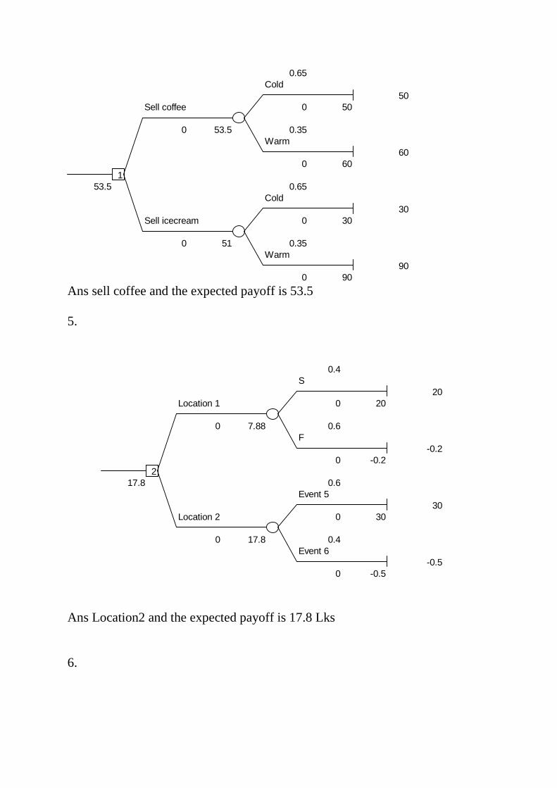
Ans sell coffee and the expected payoff is 53.5 5.

Ans Location2 and the expected payoff is 17.8 Lks 6.

0.65Cold

50Sell coffee 0 50

0 53.5 0.35Warm

600 60

153.5 0.65

Cold30

Sell icecream 0 30

0 51 0.35Warm

900 90

0.4S

20Location 1 0 20

0 7.88 0.6F

-0.20 -0.2

217.8 0.6

Event 530

Location 2 0 30

0 17.8 0.4Event 6

-0.50 -0.5

Ans Invest in Mutual Funds and the expected profit is 1.8 Crores 7. EMV = 4450/- (Expand 1000 units) Maximax – Expand 1000 units Maximin – Do not expand

0.5 3000 4500 60000.3 3000 4500 35000.2 3000 2500 2000

EMV 3000 4100 4450

0.6S

5Mall 0 5

0 -1 0.4F

-100 -10

0.7S

2Housing complex 0 2

0 1.7 0.34 F

1.8 10 1

Fixed Deposit0.9

0 0.9

0.630% Divident

3Mutual Funds 0 3

0 1.8 0.4No Dividant

00 0

EVPI = EPPI – (EMV ) max = 3.4 – 1.8 = 1.6 Crores

Mall5

0 5

0.7S

2Housing 0 2

0 1.7 0.30.5 F

Mall will be Success 11 0 1

0 5

FD0.9

0 0.9

0.630% divd

3MF 0 3

0 1.8 0.4No divd

00 0

3.4

Mall-10

0 -10

0.7S

2Housing 0 2

0 1.7 0.30.5 F

Mall will be Failure 14 0 1

0 1.8

FD0.9

0 0.9

0.630% divd

3MF 0 3

0 1.8 0.4No divd

00 0

17.17 Exercises Chapter 17 Ex. 1 . Average Value Relative = (70/50)+(130/100)+(80/40) / 3 =1.5 Ex. 2 Let q0, p0 and q1, p1 represent quantities and prices of items in 2004 and 2007. Laspeyre’s Index No. = ( Σ p1 q0 / Σ p0 q 0 )×100 = {(16×50 + 22×15 +14×20 +16×5) / (14×50 + 20×15+12×20 +14×5)} ×100 = (1080/954 )× 100 = 113.21 Paasche’s Index No = ( Σ p1 q1 / Σ p0 q1 )×100 = (16×22+22×18+14×18+16×5 ) / (14×22+20×18+12×18+14×5) ×100 = (1490/1310)×100 =113.74 Fisher’s Index No = √ {( Σ p1 q 0/ Σ p0 q0 ) × Σ ( p1 q1/ Σ p0 q1 )} × 100 = √(1490/1310 ×1080/954) ×100 = 113.47

… Ex. 3

Let the value P0 and P1 are derived as 7/1 ,5/1 , 11/1 and 18 for 2003 andP1 are derived as 7 ,5, 10 and 20 for 2006 . For Is caube workefout that Σ p0 q0 =1640 and Σ p1 q1 =1620 If caube workefout that . Proceeding as in Exercies 2 we get Σ Σ p1 q 0 =350 +600+300+400 =1650 Σ Σ p0 q1 =420+ 700 +220 +270 = 1610 L= (Σ p1 q0 / Σ p0 q1) × 100 = 1650/1640 × 100 = 100.61 P= (Σ p1 q1 / Σ p0 q1) = 1620/1610 × 100 = 100.62

F = √ 100.61 100.62 = 100.615 Σ p0 q0 = 96 , Σ p1 q 0 =129 , Σ p0 q1 = 100 , Σ p1 q1 =147 ≠ 1 Ex. 4 L =129/96 *100 =134.375 P = 147/100*100 = 147.000 F = 140 .546 Time Reversal Test : For Laspeyre’s Index : (Σ p1 q0 / Σ p0 q 0 ) ×(Σ p0 q1 / Σ p1 q1 ) = 129/96×100/147 =0.914 Ex. 5 Cost of living Index = Σ W1Q1/ Σ W1 = 50×375 + .. +13×280/ 50 +10+ ….+13 = 340.05 Ex. 6 Item Price relation

A 21/18= 1.167

B 5/4= 1.250

C 10/8= 1.250

D 4/3= 1.333

Weighted Index Number = 8×1.167 +5× 1.250 +15× 1.25+20×1.333 / 48 = ( 60.996/ 48) × 100 = 127.075 Ex 7 Year Aggregrate

Deposits( Deflated

Series)

Bank Credit(

Deflated Series)

1993-94 315132 164418 1994-95 343569.27 187886 1995-96 356759.05 208894 1996-97 397483.49 218869 1997-98 450666.42 244035

1998-99 507480.45 262144 1999-00 559769.44 300040 2000-01 618251.77 328474 2001-02 684042.16 365606 2002-03 767897.48 437179 2003-04 855267.77 477990 2004-05 907740.52 587522 2005-06 1078797.44 770883

Exs 8

Year

Consumer Price Index

1993-94 100 1994-95 110.1 1995-96 121.3 1996-97 132.6 1997-98 141.9 1998-99 160.5 1999-00 165.9 2000-01 172.1 2001-02 179.5 2002-03 186.8 2003-04 193.8 2004-05 201.6 2005-06 210.1

Ex.9 Let p0 , q 0 represent price and quantities in 2004 and p1 , q 1 represent price and quantities in 2005

p0 q 0 p1 q 1 p1 q 0 p0 q 1

128 80 144 128

120 200 160 128

500 720 600 600

180 270 180 225

928 1270 1084 1103 Laspeyre’s Index No. = 116.81 Paasche’s Index No = 115.14 Fisher’s Index No = 115.97 For Paasche’s index: Σ p1 q 1/ Σ p0 q 1× Σ p0 q 0 / Σ p1 q 0 =147/100 × 96/129 =1.094 ≠ 1 Factor Reversal Test: √Σ p0 q 1 / Σ p0 q 0 × Σ p1 q 0 / Σ p0 q 0 = √ 127/96 × 100/96 ≠ 1 For paasche’s √ Σ p1 q 1 1/ Σ p0 q 1 × Σ p1 q 1 / Σ p1 q 0 = √ 147/100 × 147/129 ≠ 147/96 Ex. 10

Year 1995 1996 1997 1998 1999 2000 2001 2002 2003 2004 2005Deflated Value of $ in

Rs. 32.42 32.806 32.15 34.99 34.46 34.826 34.12 33.93 31.446 29.01 26.51

Chapter 18 Ex.1 LCL = 99.95 − 0.577 × 8.4 = 99.95 – 4.85 = 95.10 UCL = 99.95 – 4.85 = 104.80 R = 8.4 A = R /d2 = 8.4/ 2.326 =3.611 Natural Tolerance Limits: Since natural tolerance limits are not within specification limits, process will not be able to meet the specifications. Ex. 2 C = 2 LCL = c + 3 c = 2 + 3 √2 = 6.2

UCL = c − 3 c c = 2 − 3 √2 = 0 Thus , the production line is under control . Ex. 3 Sample: 1 2 3 4 5 6 7 8 9 10 Proportion of Defectives: 0.080 ,0.185, 0.65, 0.130, 0.070, 0.120, 0.150, 0.115, 0.175, 0.070 p = 0.116 Control Limits: p ± 3√{( p q ) / n} = 0.116 ± 3√{(0.116 × 0.884)/ 200} = 0.116 ± 0.0678 = 0.0482 to 0.1838 Removing second point (0.185) p = (1.16 −.185 ) / 9 = 0.1083 Revised control limits: 0.1083 ± 3 √ {(0.1083 × 0.8917) / 200} 0.1083 + 0.660 0.0423 to 0.1743 Removing 9th point (0.175) p = 0.1 Revised control limits: 0.1 ± 3√(0.1 × 0.9) /(200) = 0.1 ± .0636 0.9394 to 0.1636 Now all eight points are under control. Ex. 4 Average no. of errors = 3.2 Control limit for number of errors = 3.2 ± 3√3.2 Since no point is outside the upper control limit i.e. 8.4, the processing of application is under statistical control . Ex. 5 Average no of rejects = 3.2 Control limits: 3.4 ± 3√3.4 i ,e 0 to 8.9 Removing point (a reject )

Average number of rejects = 59/19 = 3.105 Control limits : 3.1 ± 3√3.1 i,e 0 to 8.4 Now the process is under control . Ex. 6 Average proportion of definition s p = 17/1000 = 0.017 Control limits for proportion of defection 0.017 ± 3√(0.017 × 0.983)/100 0.0170 ± 0.0388 Upper control limit : 0.0558 No point outside limit.

Stat for Mgmt Solutions for Exercises

Documents

Transcript of Stat for Mgmt Solutions for Exercises