Stat 5100 Handout #12.f SAS: Time Series Case Study (Unit...

1

Stat 5100 Handout #12.f – SAS: Time Series Case Study (Unit 7)

Data: Weekly sales (in thousands of units) of Super Tech Videocassette Tapes over 161

weeks [see Bowerman & O’Connell “Forecasting and Time Series: An Applied

Approach”, 3rd Edition, Section 10.4 Case Study.

Goal: Want to forecast sales 25 weeks beyond end of data

/* Define options */

ods html image_dpi=300 style=journal;

data sales; input weekly @@; cards; 45.9 45.4 42.8 34.4 31.9 36.6 39.2 41.4 40.3 43.1 43.2

41.2 38.4 38.3 41.9 37.1 34.5 31.3 30.2 28.3 25.9 26.6

26.2 29 34.8 36.8 37.2 41.7 41.2 40.7 39.5 40.4 38

35.6 33.9 35.2 41.8 42.4 38.9 42.1 41.7 39.2 38.5 42.5

47.9 48.6 52 53.5 53.5 52.9 53.4 52.8 51.4 52.5 52.4

51.5 51.7 53.3 55.4 56.9 60 60.8 62.3 62.6 63.1 62.8

64.7 66.3 63 65.5 70.6 76 80.1 78.6 78.3 78.1 73.6

68.8 64.4 62.4 61.1 63.1 65.3 68.3 72.5 73.2 72.9 70.5

69.4 68.2 69.3 72.3 73.5 70.3 68.3 64.1 62.5 62.6 60.4

61.1 64.7 65.1 61.5 64.2 67.8 66.8 64.1 66.4 68 71

76.9 84.1 85.9 85.2 86.2 85.7 81.3 75.9 75 72.5 69.6

67.3 69.8 72.2 75.2 77.2 76.8 72.4 69.4 68.7 65.1 64.4

64.2 63.2 62.1 65.8 73.7 77.1 76 74.6 70.6 67.5 67.9

68.9 67.8 65.1 65 67.6 67.9 66.5 68.2 71.7 71.3 68.9

70 73.1 69.1 67.3 72.9 78.6 82.3

;

run;

/********************************************************/

/* Look at original data and check stationarity */

data sales; set sales;

Time = _N_;

proc arima data=sales;

identify var=weekly nlag=24;

title1 'Look for Stationarity in SAC; Original Time

Series';

run;

2

Look for Stationarity in SAC; Original Time Series

The ARIMA Procedure

Name of Variable = weekly

Number of Observations 161

Autocorrelation Check for White Noise

To

Lag

Chi-

Square

DF Pr >

ChiSq

Autocorrelations

6 779.33 6 <.0001 0.974 0.935 0.899 0.862 0.825 0.794

12 1366.70 12 <.0001 0.777 0.765 0.753 0.745 0.739 0.730

18 1845.25 18 <.0001 0.715 0.695 0.676 0.654 0.634 0.614

24 2177.35 24 <.0001 0.594 0.575 0.556 0.535 0.508 0.480

3

/* Remove linear effect of time */

proc reg data=sales noprint;

model weekly = time;

output out=out1 r=residtime;

proc arima data=out1;

identify var=residtime nlag=24;

title1 'Look for Stationarity in SAC; Removed Linear

Time';

run;

Look for Stationarity in SAC; Removed Linear Time


To

Lag

Chi-

Square

DF Pr >

ChiSq

Autocorrelations

6 523.89 6 <.0001 0.944 0.843 0.746 0.654 0.567 0.501

12 720.33 12 <.0001 0.469 0.447 0.434 0.427 0.422 0.409

4

/* Try to remove cyclic behavior

-- there appears to be a 2-year cycle */


sin1 = sin(2*3.14*time/104);

cos1 = cos(2*3.14*time/104);

proc reg data=sales noprint;

model weekly = time sin1 cos1;

output out=out2 r=residTimeTrig;

proc arima data=out2;

identify var=residTimeTrig nlag=24;

title1 'Look for Stationarity in SAC; Removed Linear &

Trig. Time';

run;

Look for Stationarity in SAC; Removed Linear & Trig. Time

5

/* It doesn't look like this will work

-- need to consider differencing */


weeklyd1 = weekly - lag(weekly);

weeklyd2 = weeklyd1 - lag(weeklyd1);

run;


identify var=weeklyd1 nlag=24;

title1 'Look for Stationarity in SAC; First Difference';

run;

Look for Stationarity in SAC; First Difference


To

Lag

Chi-

Square

DF Pr >

ChiSq

Autocorrelations

6 59.37 6 <.0001 0.435 -0.008 0.002 -0.017 -0.239 -0.336

6



title1 'Look for Stationarity in SAC; Second Difference';

run;

Look for Stationarity in SAC; Second Difference


To

Lag

Chi-

Square

DF Pr >

ChiSq

Autocorrelations

6 51.55 6 <.0001 -0.115 -0.408 0.047 0.190 -0.130 -0.281

7

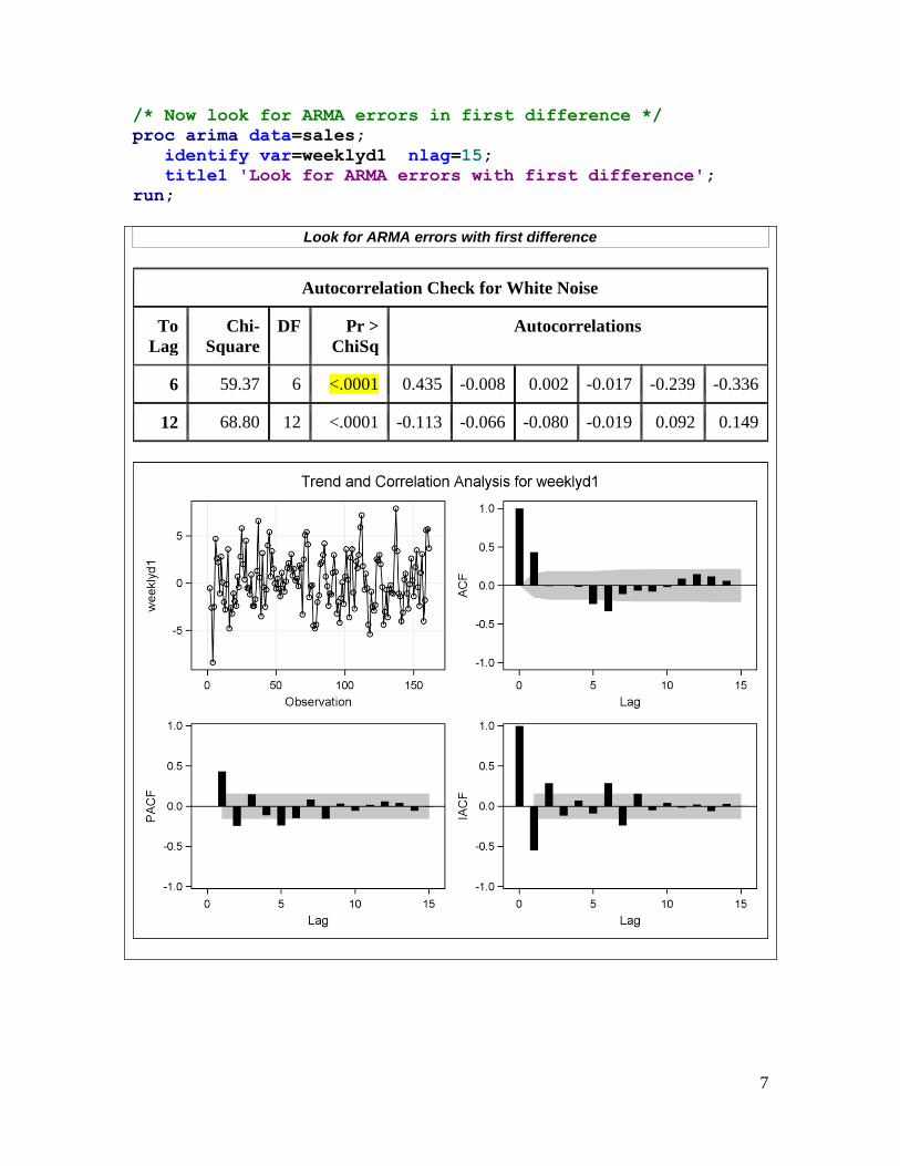
/* Now look for ARMA errors in first difference */



title1 'Look for ARMA errors with first difference';

run;

Look for ARMA errors with first difference


To

Lag

Chi-

Square

DF Pr >

ChiSq

Autocorrelations

6 59.37 6 <.0001 0.435 -0.008 0.002 -0.017 -0.239 -0.336

12 68.80 12 <.0001 -0.113 -0.066 -0.080 -0.019 0.092 0.149

8

/* Model 1: ARIMA(2,1,0), based on

SAC's damped exponential / sine pattern,

and SPAC spikes at 1 and 2 */


identify var=weekly(1);

estimate p=2 plot method=uls;

forecast lead=25 alpha=0.05 noprint out=f1;

title1 'Model 1: ARIMA(2,1,0)';

run;

Model 1: ARIMA(2,1,0)

Unconditional Least Squares Estimation

Parameter Estimate Standard Error t Value Approx

Pr > |t|

Lag

MU 0.22900 0.27904 0.82 0.4131 0

AR1,1 0.54277 0.07749 7.00 <.0001 1

AR1,2 -0.24502 0.07844 -3.12 0.0021 2

Constant Estimate 0.160818

Variance Estimate 6.147007

Std Error Estimate 2.479316

Autocorrelation Check of Residuals

To

Lag

Chi-

Square

DF Pr >

ChiSq

Autocorrelations

6 23.06 4 0.0001 0.035 -0.087 0.090 0.065 -0.151 -0.306

12 27.19 10 0.0024 0.053 -0.063 -0.074 -0.014 0.059 0.089

18 30.84 16 0.0141 0.057 0.017 0.056 -0.111 -0.019 -0.032

24 37.90 22 0.0188 0.035 -0.080 -0.058 0.140 0.034 -0.077

30 42.29 28 0.0407 0.107 0.092 -0.042 0.000 -0.030 -0.006

10

/* Model 2: ARIMA(2,1,(6)), based on

RSAC/RSPAC spikes in Model 1 */



estimate p=2 q=(6) plot method=uls;


title1 'Model 2: ARIMA(2,1,(6))';

run;

Model 2: ARIMA(2,1,(6))



Pr > |t|

Lag

MU 0.22841 0.16843 1.36 0.1770 0

MA1,1 0.34955 0.07858 4.45 <.0001 6

AR1,1 0.52984 0.07798 6.79 <.0001 1

AR1,2 -0.26407 0.07901 -3.34 0.0010 2





To

Lag

Chi-

Square

DF Pr >

ChiSq

Autocorrelations

6 7.13 3 0.0679 0.032 -0.082 0.121 0.022 -0.142 0.007

12 11.84 9 0.2226 0.085 -0.103 -0.033 -0.034 0.015 0.084

18 16.27 15 0.3645 0.114 -0.040 0.028 -0.087 -0.013 -0.041

24 23.44 21 0.3210 0.101 -0.060 -0.067 0.105 0.023 -0.092

30 29.05 27 0.3584 0.110 0.078 -0.078 0.005 -0.046 -0.050

12

/* Model 3: ARIMA(0,1,(1,6)), based on

alternative reading of first diff. SAC */



estimate p=0 q=(1,6) plot method=uls;


title1 'Model 3: ARIMA(0,1,(1,6))';

run;

Model 3: ARIMA(0,1,(1,6))



Pr > |t|

Lag

MU 0.24618 0.22800 1.08 0.2819 0

MA1,1 -0.63823 0.09741 -6.55 <.0001 1

MA1,2 0.36176 0.07368 4.91 <.0001 6





To

Lag

Chi-

Square

DF Pr >

ChiSq

Autocorrelations

6 1.76 4 0.7793 -0.000 -0.014 0.007 -0.009 -0.098 -0.026

12 6.12 10 0.8055 -0.084 0.008 -0.063 -0.061 0.059 0.083

18 10.37 16 0.8464 0.056 0.036 -0.008 -0.118 0.039 -0.062

24 16.05 22 0.8135 0.055 -0.030 -0.084 0.105 0.037 -0.083

30 21.87 28 0.7873 0.120 0.066 -0.061 0.035 -0.076 -0.019

14

/* Forecasts from Model 2: ARIMA(2,1,(6)) */

data f2; set f2;

time = _n_;

proc sgplot data=f2;

series x=time y=weekly / lineattrs=(pattern=solid

thickness=5);

series x=time y=forecast / lineattrs=(pattern=solid);

series x=time y=l95 / lineattrs=(pattern=dash);

series x=time y=u95 / lineattrs=(pattern=dash);

xaxis label='Time' values=(0 to 190 by 25);

yaxis label='Weekly Sales' values=(0 to 190 by 50);

title1 'Model 2: ARIMA(2,1,(6))';

title2 'Forecast with 95 percent confidence intervals';

run;

15

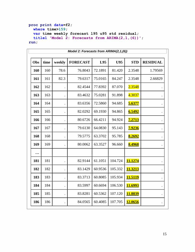
proc print data=f2;

where time>159;

var time weekly forecast l95 u95 std residual;

title1 'Model 2: Forecasts from ARIMA(2,1,(6))';

run;

Model 2: Forecasts from ARIMA(2,1,(6))

Obs time weekly FORECAST L95 U95 STD RESIDUAL

160 160 78.6 76.8043 72.1891 81.420 2.3548 1.79569

161 161 82.3 79.6317 75.0165 84.247 2.3548 2.66829

162 162 . 82.4544 77.8392 87.070 2.3548 .

163 163 . 83.4632 75.0281 91.898 4.3037 .

164 164 . 83.6356 72.5860 94.685 5.6377 .

165 165 . 82.0292 69.1930 94.865 6.5492 .

166 166 . 80.6726 66.4211 94.924 7.2713 .

167 167 . 79.6130 64.0830 95.143 7.9236 .

168 168 . 79.5775 63.3702 95.785 8.2692 .

169 169 . 80.0062 63.3527 96.660 8.4968 .

…

181 181 . 82.9144 61.1051 104.724 11.1274 .

182 182 . 83.1429 60.9536 105.332 11.3213 .

183 183 . 83.3713 60.8085 105.934 11.5119 .

184 184 . 83.5997 60.6694 106.530 11.6993 .

185 185 . 83.8281 60.5362 107.120 11.8839 .

186 186 . 84.0565 60.4085 107.705 12.0656 .

16

/* Forecasts from Model 3: ARIMA(0,1,(1,6)) */

data f3; set f3;

time = _n_;

proc sgplot data=f3;

series x=time y=weekly / lineattrs=(pattern=solid

thickness=5);

series x=time y=forecast / lineattrs=(pattern=solid);

series x=time y=l95 / lineattrs=(pattern=dash);

series x=time y=u95 / lineattrs=(pattern=dash);

xaxis label='Time' values=(0 to 190 by 25);

yaxis label='Weekly Sales' values=(0 to 190 by 50);

title1 'Model 3: ARIMA(0,1,(1,6))';

title2 'Forecast with 95 percent confidence intervals';

run;

17

proc print data=f3;

where time>159;

var time weekly forecast l95 u95 std residual;

title1 'Model 3: Forecasts from ARIMA(0,1,(1,6))';

run;

Model 3: Forecasts from ARIMA(0,1,(1,6))

Obs time weekly FORECAST L95 U95 STD RESIDUAL

160 160 78.6 76.0198 71.6123 80.427 2.2488 2.58023

161 161 82.3 80.0402 75.6328 84.448 2.2487 2.25981

162 162 . 83.4161 79.0221 87.810 2.2419 .

163 163 . 85.3235 76.8899 93.757 4.3029 .

164 164 . 85.0879 74.0000 96.176 5.6572 .

165 165 . 83.8918 70.6721 97.112 6.7449 .

166 166 . 83.2053 68.1528 98.258 7.6800 .

167 167 . 82.6389 65.9537 99.324 8.5130 .

168 168 . 82.8851 65.2824 100.488 8.9811 .

169 169 . 83.1313 64.6566 101.606 9.4260 .

…

181 181 . 86.0855 59.2746 112.896 13.6793 .

182 182 . 86.3317 58.9403 113.723 13.9754 .

183 183 . 86.5779 58.6182 114.538 14.2654 .

184 184 . 86.8241 58.3073 115.341 14.5496 .

185 185 . 87.0702 58.0071 116.133 14.8284 .

186 186 . 87.3164 57.7170 116.916 15.1020 .

18

Rough script:

0. Introduce data and express desire to forecast 25 weeks.

1. See need for stationarity based on time plot and

SAC (p. 2).

Try linear trend, see remaining ~2 year cycle (p. 3).

Try linear + trigonometric trends (p. 4).

-- But still see problems with 1st-order stationarity.

2. See stubbornness of time trends (p. 4), and need for

differencing; first diff. appears sufficient (pp. 5-6).

3. See need for dependence structure after white noise

check in first difference (p. 7).

4. Model 1: ARIMA(2,1,0), based on mixture of damped

exp. decay and sine waves in SAC, and SPAC cuts off

after lag 2 -- note may have additional spikes at lags 5

and 6 (pp. 8-9).

Goodness of fit checks: parameters significant, but

model is inadequate (p. 8).

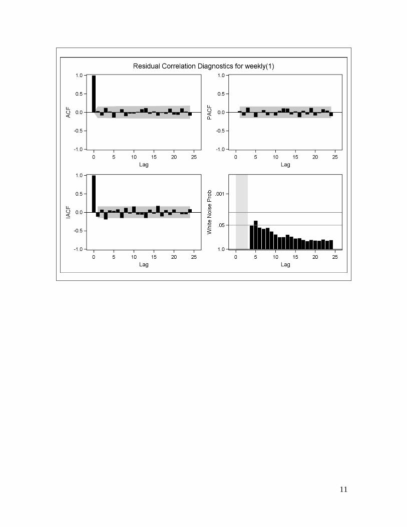
5. Model 2: ARIMA(2,1,(6)), based on spike in RSAC of

Model 1 (pp. 10-11).

Goodness of fit checks: no evidence of model

inadequacy (pp. 8-9) (? -- note Ljung-Box p-value).

6. Model 3: ARIMA(0,1,(1,6)), based on alternative reading

of SAC and SPAC of first difference -- on page 7, SAC

spikes at lags 1 and 6, SPAC dies down in oscillating

fashion. (pp. 12-13).

Goodness of fit checks: no evidence of model inadequacy

(pp. 12-13).

7. Compare forecasts from two 'adequate' models (pp 14-17):

Model 3 better only for short-term (2 week) forecasts,

based on tighter confidence intervals (smaller STD for

forecasts only for weeks 162-163).

Model 2 has tighter confidence intervals (smaller STD)

for longer-term forecasts (weeks 164-186).

Model summaries:

Model 1: S=2.48, Q=23.06 (P=.0001),

RSAC & RSPAC have spike at lag 6

Model 2: S=2.35, Q=7.13 (P=.07),

RSAC & RSPAC have 'nothing'

Model 3: S=2.24, Q=1.76 (P=.78),

RSAC & RSPAC have 'less nothing'

Conclude: Model 1 inadequate,

Model 2 best for longer-term forecasts,

Model 3 best for short-term forecasts

Stat 5100 Handout #12.f SAS: Time Series Case Study (Unit...

Documents

Transcript of Stat 5100 Handout #12.f SAS: Time Series Case Study (Unit...