Stat 315c: Transposable Data Correspondence Analysis
36
Stat 315c: Transposable Data Correspondence Analysis Art B. Owen Stanford Statistics Art B. Owen (Stanford Statistics) Correspondence Analysis 1 / 17
Transcript of Stat 315c: Transposable Data Correspondence Analysis

Stat 315c: Transposable DataCorrespondence Analysis
Art B. Owen
Stanford Statistics
Art B. Owen (Stanford Statistics) Correspondence Analysis 1 / 17
Correspondence Analysis
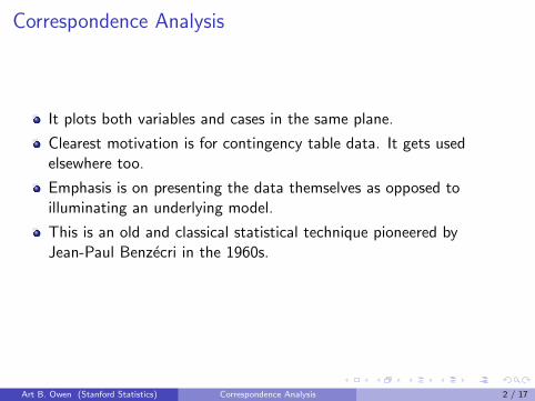
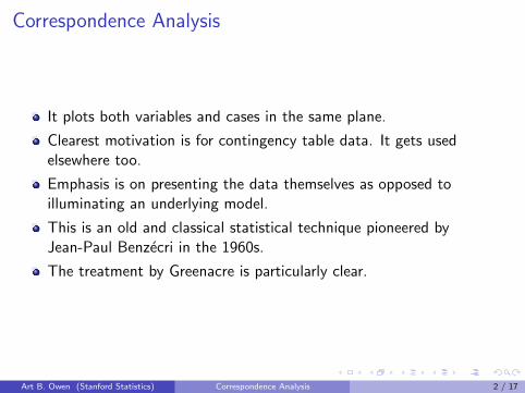
It plots both variables and cases in the same plane.
Clearest motivation is for contingency table data. It gets usedelsewhere too.
Emphasis is on presenting the data themselves as opposed toilluminating an underlying model.
This is an old and classical statistical technique pioneered byJean-Paul Benzecri in the 1960s.
The treatment by Greenacre is particularly clear.
Art B. Owen (Stanford Statistics) Correspondence Analysis 2 / 17
Correspondence Analysis
It plots both variables and cases in the same plane.
Clearest motivation is for contingency table data. It gets usedelsewhere too.
Emphasis is on presenting the data themselves as opposed toilluminating an underlying model.
This is an old and classical statistical technique pioneered byJean-Paul Benzecri in the 1960s.
The treatment by Greenacre is particularly clear.
Art B. Owen (Stanford Statistics) Correspondence Analysis 2 / 17
Contingency tables
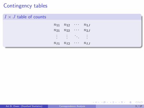
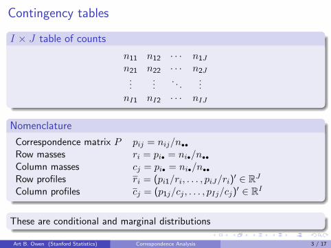
I × J table of counts
n11 n12 · · · n1J
n21 n22 · · · n2J...
.... . .
...nI1 nI2 · · · nIJ
Nomenclature
Correspondence matrix P pij = nij/n••
Row masses ri = pi• = ni•/n••
Column masses cj = pi• = ni•/n••
Row profiles ri = (pi1/ri, . . . , piJ/ri)′ ∈ RJ
Column profiles cj = (p1j/cj , . . . , pIj/cj)′ ∈ RI
These are conditional and marginal distributions
Art B. Owen (Stanford Statistics) Correspondence Analysis 3 / 17

Contingency tables
I × J table of counts
n11 n12 · · · n1J
n21 n22 · · · n2J...
.... . .
...nI1 nI2 · · · nIJ
Nomenclature
Correspondence matrix P pij = nij/n••
Row masses ri = pi• = ni•/n••
Column masses cj = pi• = ni•/n••
Row profiles ri = (pi1/ri, . . . , piJ/ri)′ ∈ RJ
Column profiles cj = (p1j/cj , . . . , pIj/cj)′ ∈ RI
These are conditional and marginal distributions
Art B. Owen (Stanford Statistics) Correspondence Analysis 3 / 17
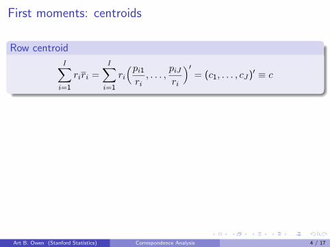
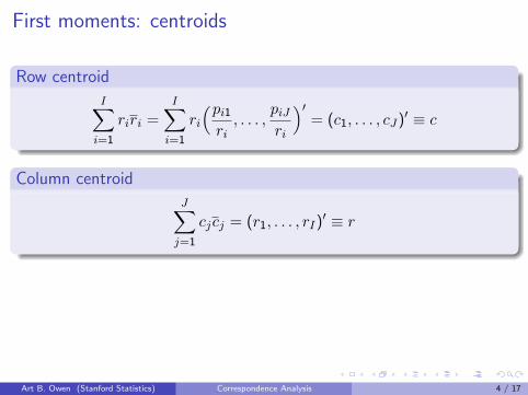
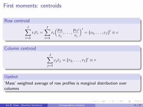
First moments: centroids
Row centroid
I∑i=1
riri =I∑
i=1
ri
(pi1
ri, . . . ,
piJ
ri
)′= (c1, . . . , cJ)′ ≡ c
Column centroid
J∑j=1
cjcj = (r1, . . . , rI)′ ≡ r
Upshot
‘Mass’ weighted average of row profiles is marginal distribution overcolumns
Art B. Owen (Stanford Statistics) Correspondence Analysis 4 / 17
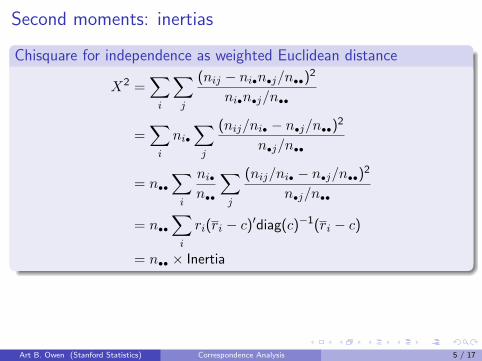
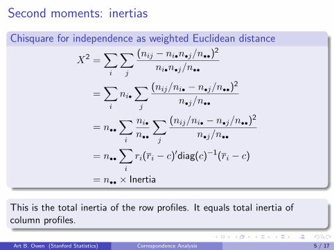
Second moments: inertias
Chisquare for independence as weighted Euclidean distance
X2 =∑
i
∑j
(nij − ni•n•j/n••)2
ni•n•j/n••
=∑
i
ni•
∑j
(nij/ni• − n•j/n••)2
n•j/n••
= n••
∑i
ni•
n••
∑j
(nij/ni• − n•j/n••)2
n•j/n••
= n••
∑i
ri(ri − c)′diag(c)−1(ri − c)
= n•• × Inertia
This is the total inertia of the row profiles. It equals total inertia ofcolumn profiles.
Art B. Owen (Stanford Statistics) Correspondence Analysis 5 / 17
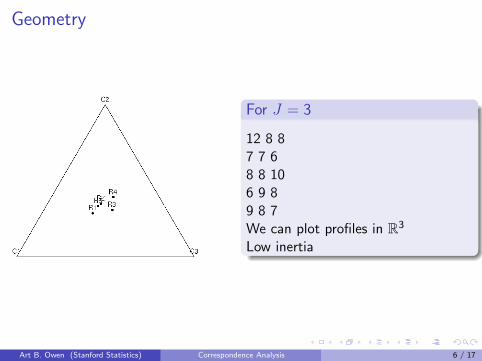
Geometry
For J = 3
12 8 87 7 68 8 106 9 89 8 7We can plot profiles in R3
Low inertia
Art B. Owen (Stanford Statistics) Correspondence Analysis 6 / 17
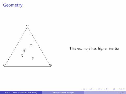
Geometry
This example has higher inertia
Art B. Owen (Stanford Statistics) Correspondence Analysis 7 / 17
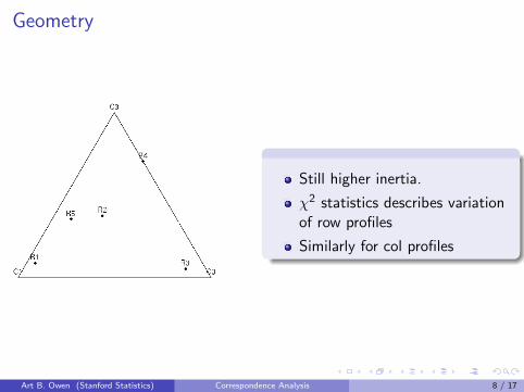
Geometry
Still higher inertia.
χ2 statistics describes variationof row profiles
Similarly for col profiles
Art B. Owen (Stanford Statistics) Correspondence Analysis 8 / 17
Rescale
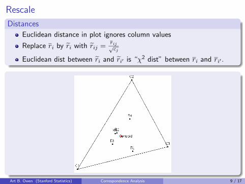
Distances
Euclidean distance in plot ignores column values
Replace ri by ri with rij =rij√cj
Euclidean dist between ri and ri′ is “χ2 dist” between ri and ri′ .
Art B. Owen (Stanford Statistics) Correspondence Analysis 9 / 17
Rescale
Distances
Euclidean distance in plot ignores column values
Replace ri by ri with rij =rij√cj
Euclidean dist between ri and ri′ is “χ2 dist” between ri and ri′ .
Art B. Owen (Stanford Statistics) Correspondence Analysis 9 / 17
Reason for χ2
Invariance
Suppose rows i and i′ are proportional
nij/ni′j = α all j = 1, . . . , J
Suppose also that we pool these rows
New ni∗j = nij + ni′j
and delete originals
Then
New χ2 distance between cols j and j′ equals old dist
Principle of distributional equivalence
Common profile, summed mass
Role of χ2 in statistical significance is not considered important in thisliterature
Art B. Owen (Stanford Statistics) Correspondence Analysis 10 / 17
Dimension reduction
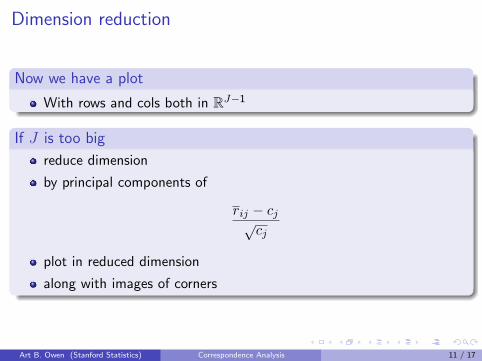
Now we have a plot
With rows and cols both in RJ−1
If J is too big
reduce dimension
by principal components of
rij − cj√cj
plot in reduced dimension
along with images of corners
Art B. Owen (Stanford Statistics) Correspondence Analysis 11 / 17
Dimension reduction
Now we have a plot
With rows and cols both in RJ−1
If J is too big
reduce dimension
by principal components of
rij − cj√cj
plot in reduced dimension
along with images of corners
Art B. Owen (Stanford Statistics) Correspondence Analysis 11 / 17
Duality
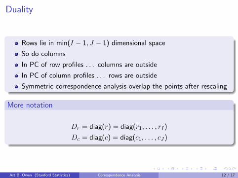
Rows lie in min(I − 1, J − 1) dimensional space
So do columns
In PC of row profiles . . . columns are outside
In PC of column profiles . . . rows are outside
Symmetric correspondence analysis overlap the points after rescaling
More notation
Dr = diag(r) = diag(r1, . . . , rI)
Dc = diag(c) = diag(c1, . . . , cJ)
Art B. Owen (Stanford Statistics) Correspondence Analysis 12 / 17
Duality
Rows lie in min(I − 1, J − 1) dimensional space
So do columns
In PC of row profiles . . . columns are outside
In PC of column profiles . . . rows are outside
Symmetric correspondence analysis overlap the points after rescaling
More notation
Dr = diag(r) = diag(r1, . . . , rI)
Dc = diag(c) = diag(c1, . . . , cJ)
Art B. Owen (Stanford Statistics) Correspondence Analysis 12 / 17
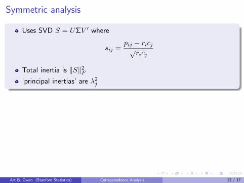
Symmetric analysis
Uses SVD S = UΣV ′ where
sij =pij − ricj√
ricj
Total inertia is ‖S‖2F
’principal inertias’ are λ2j
Coordinates
Rows (1st k cols of)
F = (D−1r P − 1c′)D−1
c V1:k = D−1r UΣ
Columns (1st k cols of)
G = (D−1c P − 1r′)D−1
r U1:k = D−1c V Σ′
Art B. Owen (Stanford Statistics) Correspondence Analysis 13 / 17
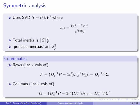
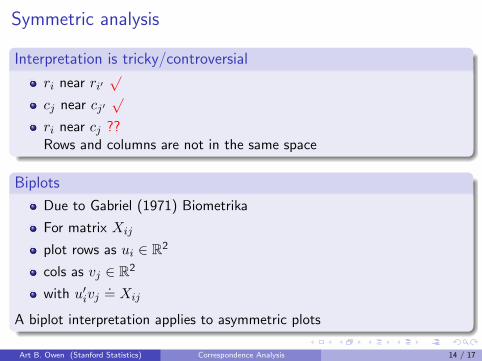
Symmetric analysis
Interpretation is tricky/controversial
ri near ri′√
cj near cj′√
ri near cj ??Rows and columns are not in the same space
Biplots
Due to Gabriel (1971) Biometrika
For matrix Xij
plot rows as ui ∈ R2
cols as vj ∈ R2
with u′ivj.= Xij
A biplot interpretation applies to asymmetric plots
Art B. Owen (Stanford Statistics) Correspondence Analysis 14 / 17
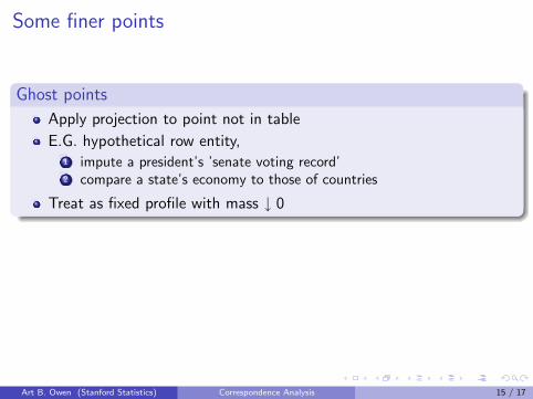
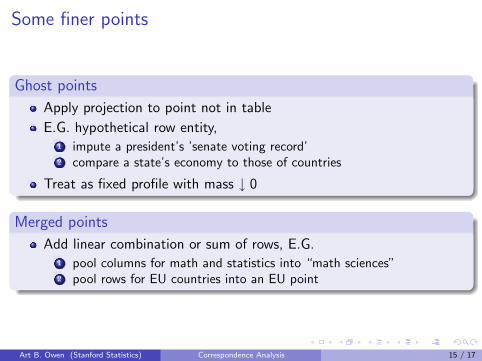
Some finer points
Ghost points
Apply projection to point not in table
E.G. hypothetical row entity,1 impute a president’s ’senate voting record’2 compare a state’s economy to those of countries
Treat as fixed profile with mass ↓ 0
Merged points
Add linear combination or sum of rows, E.G.1 pool columns for math and statistics into “math sciences”2 pool rows for EU countries into an EU point
Art B. Owen (Stanford Statistics) Correspondence Analysis 15 / 17
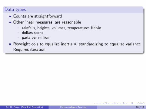
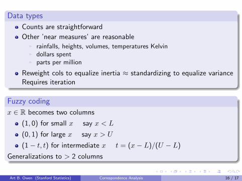
Data types
Counts are straightforward
Other ’near measures’ are reasonableI rainfalls, heights, volumes, temperatures KelvinI dollars spentI parts per million
Reweight cols to equalize inertia ≈ standardizing to equalize varianceRequires iteration
Fuzzy coding
x ∈ R becomes two columns
(1, 0) for small x say x < L
(0, 1) for large x say x > U
(1− t, t) for intermediate x t = (x− L)/(U − L)
Generalizations to > 2 columns
Art B. Owen (Stanford Statistics) Correspondence Analysis 16 / 17
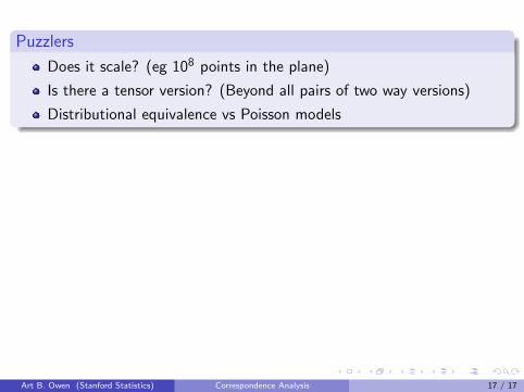
Puzzlers
Does it scale? (eg 108 points in the plane)
Is there a tensor version? (Beyond all pairs of two way versions)
Distributional equivalence vs Poisson models
Further reading
“Correspondence Analysis in Practice” M.J. Greenacre, 1993Emphasizes geometry with examples
“Theory and Applications of Correspondence Analysis” M.J.Greenacre, 1984Good coverage of theory with examples
“Correspondence Analysis and Data Coding with Java and R” F.Murtagh, 2005Code and worked examples
Art B. Owen (Stanford Statistics) Correspondence Analysis 17 / 17